the Creative Commons Attribution 3.0 License.
the Creative Commons Attribution 3.0 License.
Defining and analyzing the frequency and severity of flood events to improve risk management from a reinsurance standpoint
Elliott P. Morrill
Joseph F. Becker
The National Flood Insurance Program (NFIP) debt has accelerated research into private flood insurance options. Offering this coverage begins with the ability to transfer the risk to the reinsurance market. Within the industry, perils such as hurricanes and earthquakes have standard definitions, but no such definition exists for floods. An event definition must examine the spatial and temporal aspects of the flood as well as the complexities of individual events. In this paper we were able to apply a data-driven methodology to capture and aggregate flood peaks into independent events. To aggregate flood peaks into independent events we needed to define what constituted a basin as our area of aggregation. The USGS utilizes the hydrological unit code (HUC) a 2- to 12-digit code that follows the Pfafsetter Coding System. The HUC code is used to identify varying levels of basin sizes ranging from region (2 digits) to subwatershed (12 digits). We chose to analyze both the HUC8 and HUC6, and a total of 7932 HUC8 events and 8444 HUC6 events were recorded during the 15 water years used in our study. Each event was characterized by duration, magnitude and severity. Focusing on the HUC8, events were unevenly distributed nationally while severity was relatively evenly distributed. The goal for our study was to take a method and be able to apply it to basins of varying characteristics. This framework relied on the ability to analyze the individual processes related to each individual basin.
- Article
(5314 KB) - Full-text XML
-
Supplement
(71 KB) - BibTeX
- EndNote


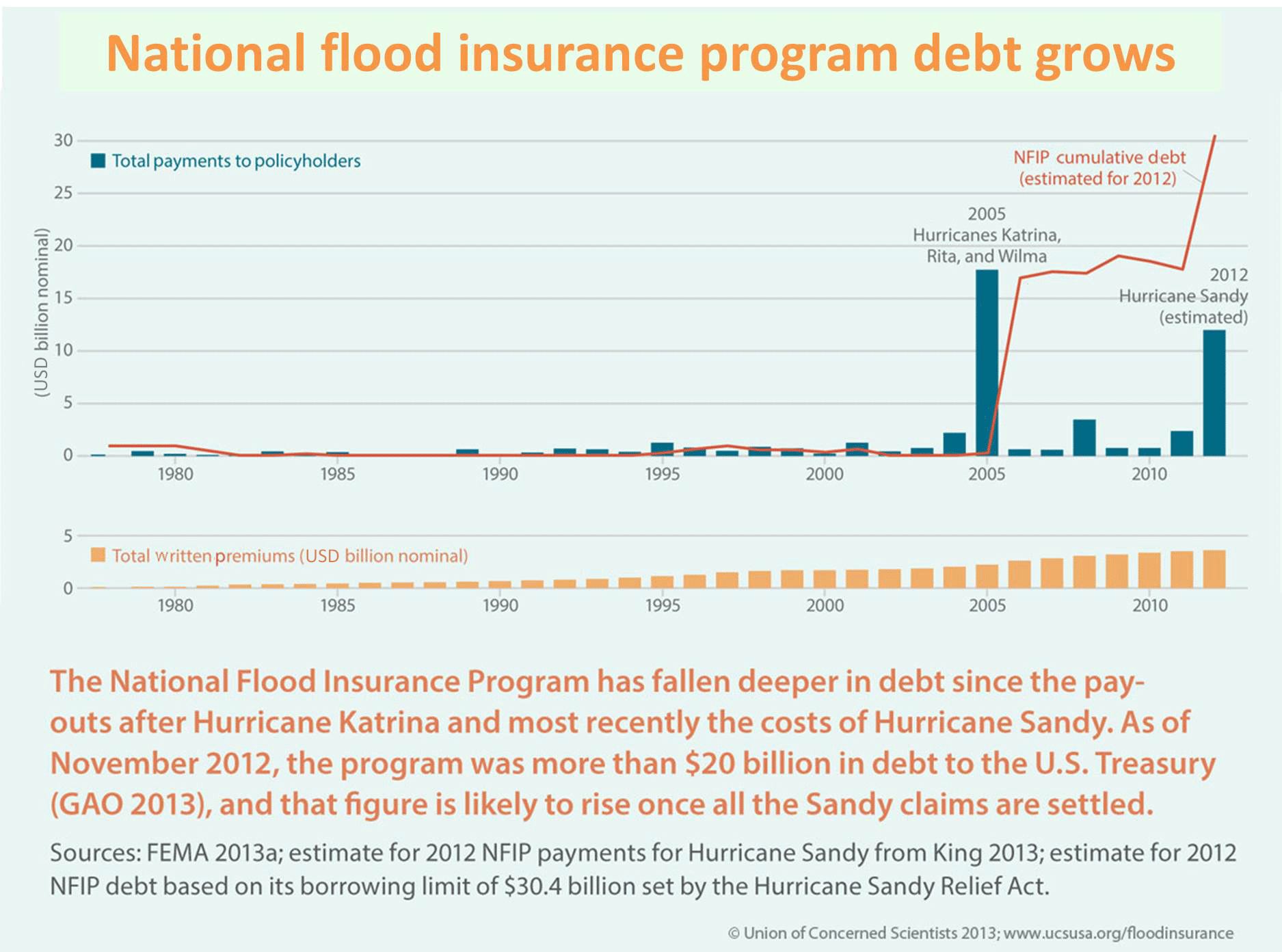
Throughout the world, flood events are one of the most destructive natural disasters. Floods occur for a variety of reasons, and risk factors such as total rainfall, soil types and land use can contribute to the complexity of events, in particular impacted area and event duration (Uhlemann et al., 2010). Every year, major and minor floods contribute to economic and insured losses (Joyce, 2014; FEMA, 2016). In the United States, the National Flood Insurance Program (NFIP) is the primary provider for residential flood insurance. Since its inception in 1968, the NFIP premiums have largely covered the amount paid out in losses (NFIP Act of 1968). However, the 2005 hurricane season, including Hurricane Katrina, which was the costliest storm in the program's history, costing more than USD 16 billion, pushed the NFIP into debt (Fig. C1) (Union of Concerned Scientists, 2016). The NFIP debt was exacerbated by the significant property damage experienced during Superstorm Sandy in 2012. Currently, the NFIP debt is estimated at USD 24 billion as of 2014 (Joyce, 2014).
This extreme debt has accelerated research into a number of different private flood insurance options. One necessary issue to address before primary flood insurance can become a more standard offering is the ability to transfer risk to the reinsurance community. A challenge specific to flooding is the complexity of individual events. Unlike the perils with an unambiguous event definition, such as hurricanes and earthquakes, there is no standard definition for a flood event, which can range in length from hours to months. The problem for flooding is not specific to the United States. In fact, reinsurers have offered flood risk transfer products in Europe and Asia for a number of years. For example, (re)insurers in Spain have provided flood insurance since 1971 (Barredo et al., 2012). Typically, reinsurance contracts define a flood event using an hours clause ranging between 168 h in the UK to 504 h in Germany. Using the hours clause insurance companies are able to aggregate claims during this period of time to limit cumulative losses from multiple events (Karnbaum and Kron, 2005). Defining events this way allows for providers to aggregate claims that can be associated with the same temporal event.
However, the hours clause definition lacks the ability to discern between the shorter and longer events. Not all events can fit into a single defined time frame. If there are multiple short-duration events occurring in quick succession then the claims from those events may be aggregated together. The hours clause also lacks the ability to determine spatial aspects of each flood event. If events occur within the same window of time but in two different areas those floods are still attributed to one event. Aggregating these events limits the ability to understand the spatial extent based on impacted areas and the severity of each of the individual flood occurrences.
While research into flood event definitions is accelerating, it is not a novel topic. Research into event definitions has primarily focused on single site analysis (Bacova-Mitkova and Onderka, 2010; Mallakpour and Villarini, 2015, 2016; Kahana et al., 2002). However, as flood events are spatially complex, they often impact many locations, limiting the use of single-site definitions for reinsurance contract definitions. When events impact larger areas, multiple locations or entire basins, there is currently no method that can properly group flood peaks to the same event.
Public entities have compiled databases of flood occurrences to assist in frequency and severity analyses (e.g., the National Climatic Data Center, NCDC). One goal of this type of analysis is to determine if floods are occurring more often and with increased severity due to climate change or other anthropogenic causes (Himmelsbach et al., 2015). Public databases are comprised of documentary sources and trained spotter observations (NCDC, EM-Dat, and DFO). The major downside of using this type of database to assist with reinsurance contracts is that they are based on subjective measures such as spotter definitions. Definitions follow a series of guidelines but varying flood characteristics between regions can categorize flooding differently between these two regions. Variations in categorization have an impact on event durations and impacted areas. In addition to the definitions themselves, trained spotters respond to citizens reports of the peril. Depending on the area, what is considered abnormal flooding, in terms of standing water or bank-full discharge, may be reported in one area and not in another. For example an area such as Florida experiences significant precipitation year round, which may contribute to minor flooding that is considered normal and thus not reported. However in an area like Los Angeles that similar minor flooding may be reported, which affects the frequencies of flooding in each area. Another source of flood occurrence information is using a documentary source, which involves examining media sources as well as government reports to comprise a set of occurrences across a state, a country or the globe (Himmelsbach et al., 2015; Doocy et al., 2013). These sources rely heavily on the quality of the reporting, using the reports to assign severity and frequency estimates to cover an expansive region.
Relying solely on visual reports can lead to three main areas of inconsistencies in flood observations. Firstly, multiple sources can report statistics about an individual event that drastically vary in the event details, and determining the accuracy of conflicting points is challenging without additional information. Secondly, relying on trained spotter reporting to accurately define an event is problematic. In many cases the reports cover the first instance of flooding and associated damages but do not report flooding on subsequent days, which should logically define the event duration. Finally, determining the size of an event requires insight from the entire domain that was flooded. Relying solely on trained spotters may only confirm flooding in areas that contain the most crucial infrastructure or areas of interest, leading to underestimation of the entire flood extents.
EM-DAT and NCDC Storm Data databases are the two most commonly used datasets for this type of analysis. EM-DAT uses official records of areas affected, persons killed, disaster declarations issued and calls for international assistance made (Doocy et al., 2013). The NCDC Storm Data database is a compiled set of observations from National Oceanic and Atmospheric Administration (NOAA) trained spotters. NCDC events are categorized by county and then separated by dates (Dobour and Noel, 2005; Gaffin and Hotz, 2000). EM-DAT catalogues events by year with summary statistics detailing frequency and overall event impacts (i.e., deaths and losses) from that year. Such summary statistics include injured, affected, total deaths and total damage. Both methods contain a number of different biases preventing use in reinsurance contracts including population biases, frequency biases and reporting biases. Due to the incomplete and often inconsistent reporting, implementing this method to formulate an event definition for reinsurance contracts presents a challenge. Despite their limitations, these datasets are useful first checks when developing a more robust method to define flood events that historical events can be compared to.
Many authors have shifted toward a data-driven approach using the peak-over-threshold (POT) analysis to examine changes in flood event frequency (Mallakpour and Villarini, 2016; Bacova-Mitkova and Onderka, 2010), as well seasonality (Black and Werritty, 1997). A data-driven approach allows for the definition of an event to encompass a variety of basin characteristics. Authors choose a somewhat arbitrary threshold where if a peak observation exceeds the threshold, it is considered to be a POT. A subsequent step for this method was to determine a metric for identifying independent peaks. Varying windows of time were used to identify the independence between the individual POT. Mallakpour and Villarini (2016) used an arbitrary window of 15 days, where any peak that occurs within this period is aggregated to a single event. Black and Werrity (1997) determined their window by calculating the “time to rise” and identifying when the discharge dropped below two-thirds of the previous peak. Authors using these windows then looked at all individual peaks occurring within these windows to attribute them to the same event.
Site-specific event identification is the base in developing a consistent method of event identification. However, our method will address the window of independence through an observational approach. Event independence should not be based on a standard window (Mallakpour and Villarini, 2016). It must be based on how each site reacts to the flood waves. Implementing a concept similar to time to rise and a drop in discharge (Black and Werritty, 1997) was the first of many steps taken toward resolving this. The window must cover the time before and after a peak, as previous peaks have an influence on succeeding peaks. Incorporating this into our definition will reflect the individuality of each site and the flexibility of our definition to cover a wider range of sites.
The primary goal of this research is to expand our definition to an entire basin or catchment area. These regionally impacting events are titled basin or “trans-basin” events (Nied et al., 2014; Uhlemann et al., 2010). Both papers used the POT method as well. Starting with a single site, individual events were identified (Uhlemann et al., 2010) and then all mutually dependent events were identified from a moving temporal window. The window defined from previous literature provides a solid structure but categorizes catchments and basins into an all-encompassing time frame. A more basic-specific time frame is measurable and would not underestimate the smaller basins or overestimate the larger basins.
This paper seeks to define events through a data-driven approach aimed at accounting for the individuality of flood waves and the basins they impact. Our main goal is to develop a consistent definition in order to examine how frequency and severity vary regionally. Looking at frequency regionally provided us with a clearer picture of the specific areas that were more at risk for flooding. Severity allowed us to look at how areas with similar frequencies were experiencing events in terms of impacted areas and overall magnitude. Severity will factor into future implementation of risk-mitigating factors that can look at two areas and determine the steps needed to protect a certain area. It also allowed us to determine if our method is representing more local or extreme flooding across the various basins.
Methods implementing the hours clause or standard event windows lack the ability to interpret how each individual flood wave progresses. Understanding the individuality of the flood is the basis for how our method will tackle a standard event definition. This paper will be structured as follows: Sect. 2 will cover the data availability as well as the data selection process along with which tools were used to analyze the data. The concepts that feed into our method as well as our method itself will be discussed in Sect. 3. Section 4 will provide the results of the analysis from our methodology with comparisons to methodologies exhibited in previous research. Section 5 will provide the discussion and concluding remarks regarding our results within this study.
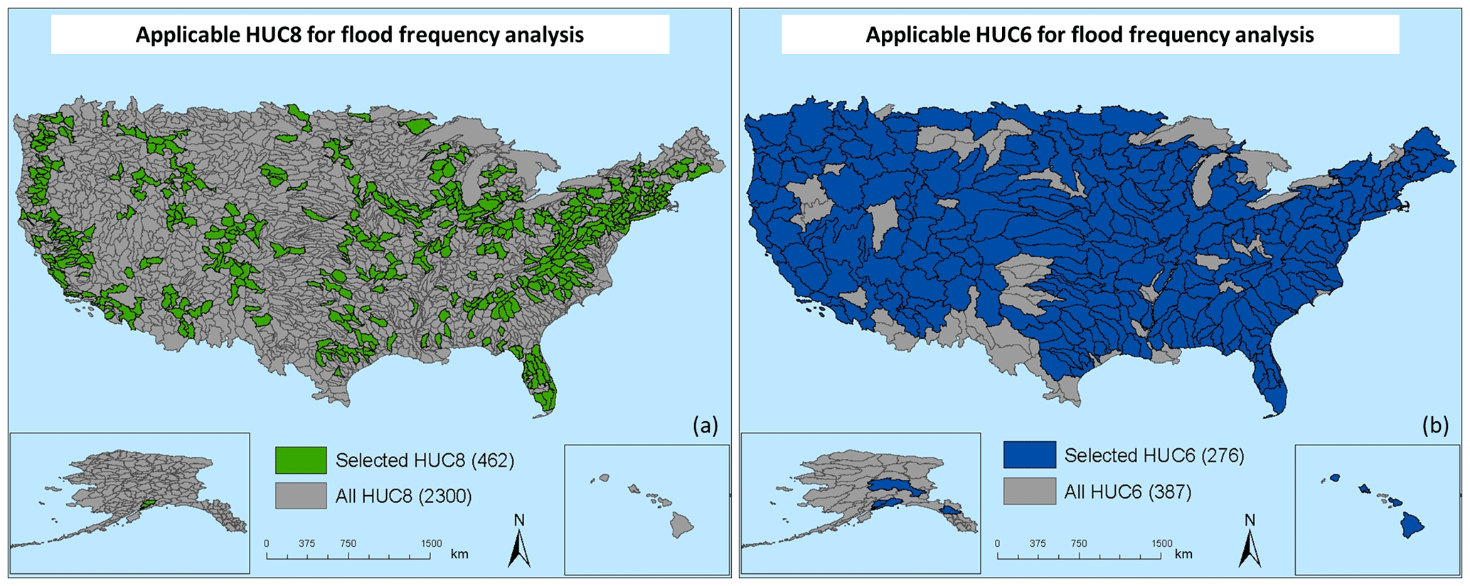
This research focuses on expanding the definition of a flood event from an individual site to river basin. As this research focuses on the United States, USGS daily flow gauges stations were used to identify individual sites and USGS hydrological unit codes (HUCs) were used to define river basins. River basins can be defined in a number of ways and determining the appropriate size can be a nontrivial task. For use in reinsurance contracts, river basins should be defined in such a way that flooding events within a portion of the basin show a correlation to events in other portions of the same basin. Basins will also need to be defined in such a way that we can see how flood waves impact the entire basin and not individual sections of that basin. The USGS HUC codes follow the concept of the Pfafstetter Coding System, meaning that each unit code is delineated in a hierarchical fashion ranging from larger to smaller. Drainage areas are defined on a continental scale and then divided and subdivided into six levels. Each level is associated with a number of digits corresponding to size. The USGS utilizes a 2 digit system that defines each basin level by the number of digits each code contains. HUC Codes range from 2 to 12 digits, largest to smallest (USGS). For example, each basin defined as a HUC8 (subbasin) has a unique 8-digit code. Based on this system as well as past research, the 8- and 6-digit HUCs were chosen as the basin levels that we would analyze. A majority of the papers that we referenced in this study have dealt with European or Asian basin definitions and were focused on one or two basins within a finite area. With our broad scope of study, we needed to look at basins across a variety of characteristics, so a common basin code was needed for comparisons of frequency. Other research of flood frequency did not yield any references to the HUC basin codes so as authors we developed our own criteria that we felt best represented the size of the basins most applicable for our methodology. Our decision to use these two sizes of HUC was based on looking for a basin size that allowed us to observe how the events would aggregate to a basin-level event rather than being identified as two separate events. We wanted our dataset to contain the largest percentage of HUCs possible after our site selection criteria to get a better nationwide picture of how our method observed basin-wide flood events. With the HUC8 we were able to get approximately 20 % of coverage across the United States with a basin contained all 20 HUC2s (Fig. 1). With any HUC size below the HUC8 such as the HUC10 we were left with a much lower coverage percentage, roughly less than 10 % for the HUC10, which would not accurately represent the methodology across the country. When we looked at the upper end of our HUC size for the HUC6, we looked at how frequency compares with site count above the HUC6 we saw that frequencies were heavily affected by site count. From these two factors we felt that the HUC8 and HUC6 were the most applicable basin sizes. Daily mean discharge as well as annual peak streamflow was used for all sites, which provided data for those parameters.
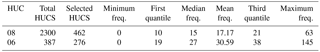
From all available HUCs, sites and basins were selected based on a number of selection criteria. The first criterion removed sites with less than 5 years of daily discharge data. The second criterion required sites to occur along natural rivers and streams; gauges impacted by reservoirs and other impediments to natural flow were excluded. Following site removal, HUCs with less than five sites were excluded. Finally, HUCs were required to have at least three sites that overlapped with 70 % of the data during each individual year that was examined. Due to the nature of our method seeking to aggregate peaks from multiple sites, the sites needed to overlap or else that method would be looking primarily at individual site events instead of the basin events. Of the 2300 HUC8s and 387 HUC6s available, 462 HUC8s and 276 HUC6s were used (Fig. 1) with a total of 3121 and 4919 gauge stations within the HUC8 and HUC6 respectively. Both HUC sizes were analyzed for initial frequencies and the most applicable HUC was chosen for subsequent analyses.
Daily discharge data from 8084 river gauge stations were obtained from the USGS (http://nwis.waterdata.usgs.gov/nwis/dv/?referred_module=sw, last access: June 2016). A study period of 15 water years between 2000 and 2015 was selected for this analysis. Initial attempts to expand the period of analysis severely reduced the number of basins that met the criteria for analysis. The peak-over-threshold method outlined in Uhlemann et al. (2010) was conducted on all basins that fit the criteria for analysis. The peak-over-threshold method consists of identifying individual observations over a specified threshold within a particular time window. The procedure was split into four major steps: (1) identifying peaks occurring at each site within each basin and the subsequent peaks over threshold; (2) applying a window of independence at each site to determine independent site-specific events; (3) compiling all independent site-specific events and applying a secondary window of independence to determine independent basic-specific events; and (4) applying multiple characteristics to determine a severity score to compare differing events from one another.
The first step involved selecting a minimum threshold. The median of annual maximums was chosen as the threshold in which a flood peak must exceed. The median of annual maximums was chosen because it corresponds to the 2-year quantile, or Q2. Uhlemann et al. (2010) states that the “Q2 is a rough estimation for bank-full discharge on naturally occurring streams”. For sites with at least 5 years of annual peak streamflow data, their Q2 was calculated by taking the median across the entire time series. As peak discharges are determined by instantaneous measurements, small catchments can exhibit extreme values, which are rarely observed in the daily record. The extreme values may lead to a minimum threshold that may not be a representative measurement of flooding for that catchment area. The discharge values at each of the peaks recorded were then compared to their respective sites' Q2 value to determine all of the peaks over threshold.
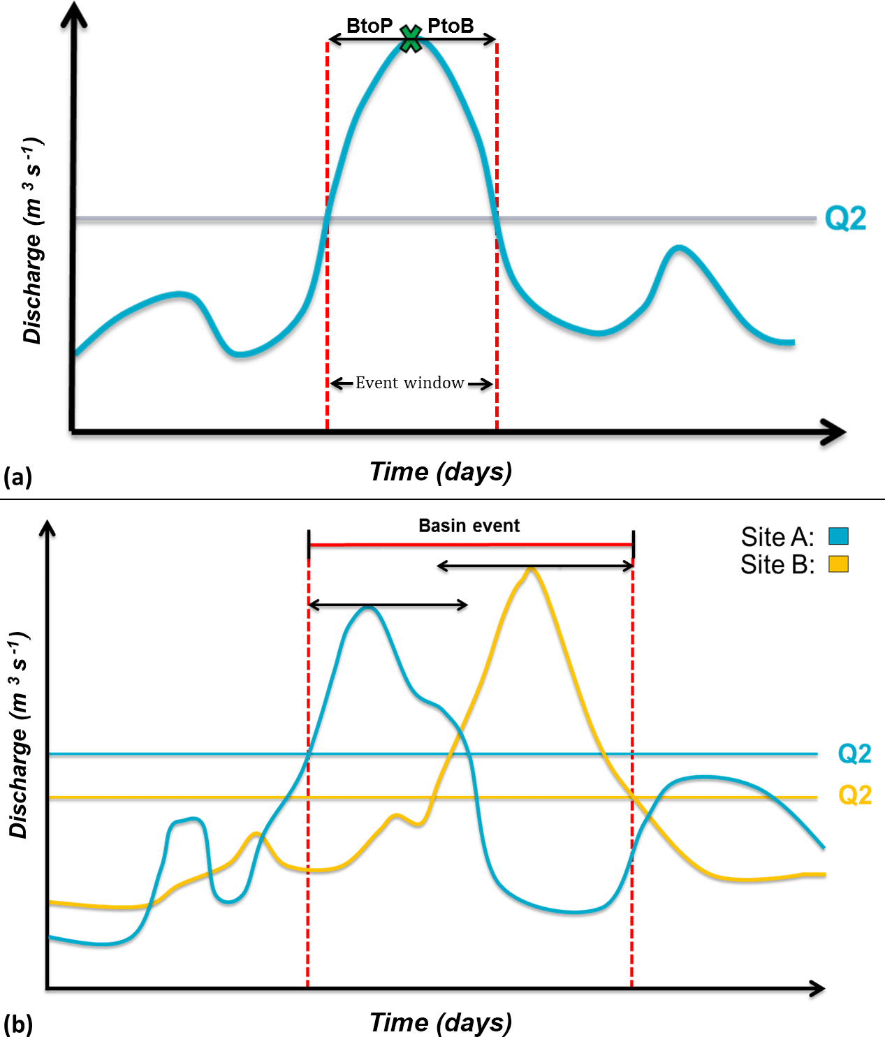
The next step in identifying site-specific events is to determine a time criteria that defines independent site events. Two metrics were calculated for all peaks over threshold to determine the duration of each event: base to peak (BtoP) and peak to base (PtoB). Base to peak is the time it takes for the discharge to reach the peak after it has crossed the minimum threshold. Peak to base is the amount of time it takes for the discharge to return to the minimum threshold following a peak (Fig. 2a). In the case where there are multiple peaks before the discharge returns to base, the peak was selected as the observation that experienced the maximum discharge. Each peak over threshold has a unique BtoP and PtoB that could have a significant range. To standardize the windows of independence for each site the median of both metrics was calculated and then the peaks start and end times were recalculated. Our window of time was aimed at eliminating the extreme events on either end of the temporal distribution to determine a window that reflected the time it would take for a flood wave to progress through a site.
After the windows were recalculated, combining peaks with overlapping or consecutive windows into a single site-specific peak-consolidated peaks. All peaks over thresholds with windows that did not overlap were treated as independent events. Each event was characterized by site number, start time, peak time, end time and peak discharge. For the peaks, which overlapped, the start time was defined as the earliest start day and end time was the latest end date. The peak discharge from each event was then scaled by the Q2 at each site. Scaling each peak discharge reduced the impact of catchment size when comparing magnitude of discharge and made the different sites comparable.
A similar methodology of consolidating overlapping observations was applied to define basic-specific events from the site-specific events (Fig. 2b). The basic-specific events used the start and end time of each site-specific event that occurred within the basin. If the windows of time between the start and end of the site-specific events overlapped or were consecutive (i.e., occurred within 1 day of another peak), then these events comprised one basic-specific event. The start of the event was the earliest start time recorded at any site and the end of the event was the final end time recorded. Each event was defined by start time, end time, peak time, and peak discharge for all events from the desired HUCs.
The final step involved in determining a severity score for each basin event. Defining severity allowed us to compare areas of like frequency. From these we were able to see that certain areas that are more vulnerable during flooding. Severity scores in future analyses will also factor into pricing of reinsurance contracts. Severity of each event was designed to include elements of the spatial extent as well as the magnitude of the flooding experienced in the basin by the affected sites during each event. The severity score represents a number between 0 and infinity where the high value indicates a more severe event. The affected sites were defined as the number of sites within the desired HUC, which recorded a peak over threshold during the event. Total discharge was the sum of the discharges, scaled by their corresponding minimum threshold, observed at all the affected sites. Severity was calculated by taking the sum of all scaled discharges and dividing by the total number of sites within the basin, Eq. (A1). If a site was impacted more than once during a basin event, the maximum-scaled discharge was selected to calculate the severity score. Scores less than 1 are expected when looking at the minimum threshold as it represents small-scale and localized flooding, in terms of discharge and the percentage of sites it may impact within the individual HUC.
From the analyses, we compared the HUC6 and the HUC8 frequencies, event duration and severity distributions. With our goal of a basin-wide definition, it is imperative to compare these two basin sizes and determine the most appropriate basin level for our methodology. To compare, we looked at the differences between the statistics listed previously as well as the distribution of the percentage of impacted sites by event for each HUC. The distribution of the percentage of impacted sites was used to determine whether events in each basin level are being aggregated to a basin event or if they are being segmented due to the size of the basin.
Two comparisons were made to the NCDC Storm Data. The first method looks at all reports of flooding and aggregates them by county. The second method used a standard 13-day independence window, 3 days prepeak and 10 days postpeak (Uhlemann et al., 2010). A standard window was used because the NCDC observations are unable to provide a site-specific window of independence.
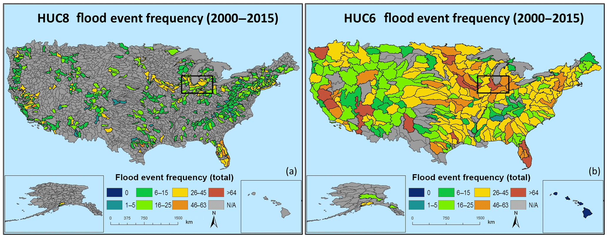
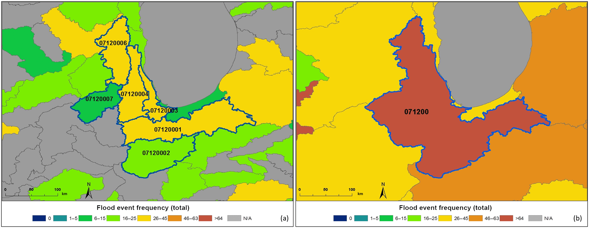
Figure 4HUC8 and HUC6 frequency comparison, upper Midwest. Blue outline (HUC6: 071200, HUC8: 07120001–07120007).
A total of 7932 and 8444 events were calculated for basins defined by the HUC8 and HUC6 respectively. Table B1 provides the frequency summary statistics for both the HUC8 and HUC6 basins. Comparing the frequency distribution of events between the two selected basins' sizes suggests that frequencies within basins defined by the HUC6 are higher than frequencies defined by the HUC8 (Figs. 3 and 4). We can see that from Fig. 3, the frequencies in each HUC8 are typically lower than the frequencies found in each HUC6. This is highlighted in Fig. 4, where we focus on six HUC8s that make up one HUC6 (outlined in blue). From here the individual basins in the HUC8 indicate a lower basin-level frequency than at the HUC6. This comparison is important because the aim of this paper is to define events at a basin level by aggregating individual events into basin-wide events. To explore this concept more we wanted to look at the impacted sites during the events compared to the total number of sites within the basin to get a sense of how many events are being determined as local when they should be aggregated. While there will be a number of small local floods that this methodology captures, we looked at this to provide us with an indication of whether the HUC8 is too small of a basin to use or the HUC6 is too large.
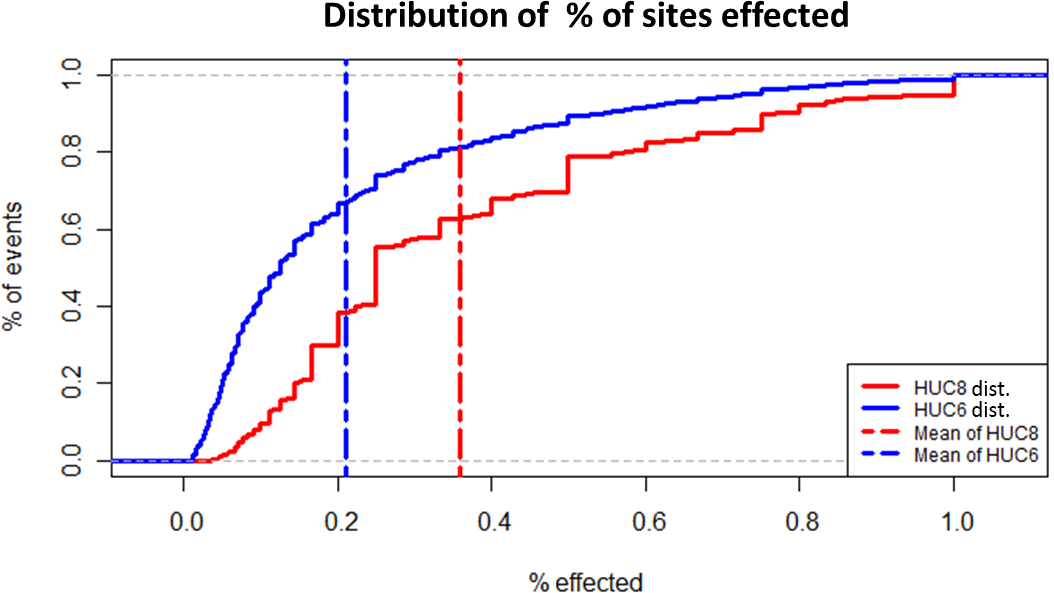
Figure 5CDF of the percentage of sites impacted during each event within our catalog. Mean % of the entire distribution is noted and split by HUC.
We looked at the distribution of the percentage of impacted sites by event for each HUC (Fig. 5). We took each event within our catalog and identified how many sites were impacted. The percentage impacted was calculated by taking the number of sites impacted and dividing by the total number of sites within the basin. For the events within the HUC8 on average 36 % of the sites were impacted compared to 21 % for the HUC6. When you look at the CDF of the events of HUC6 and HUC8 (Fig. 5), we can clearly see that the HUC6 events impact a smaller percentage of sites. While HUC6 does have more sites, due to our methods' intended aggregation of events we would expect a similar percentage of sites impacted between the two. However, because the HUC6 is showing a lower percentage of sites impacted during the events in their catalog this is an indication that the HUC6 does not aggregate individual events as well as the HUC8. A total of 80 % of the events within the HUC6 impacted < 40 % of the sites, compared to the HUC8 where approximately 50 % of their events are impacting 50 % of the sites. Due to the size of the HUC6, the basin is being segmented during our method and is not capturing events that should be attributed to the same event. The segmentation of the events within the basin will lead to an overstating of the frequencies. Overall, the HUC8 is showing a higher percentage of events in the higher percentages of sites impacted, meaning that our method is aggregating more individual events into basin events at this basin level when compared to the HUC6. From both the CDF and the average we have concluded that the HUC8 is a more applicable basin size due to its ability to aggregate the events within the basin rather than segmenting them.
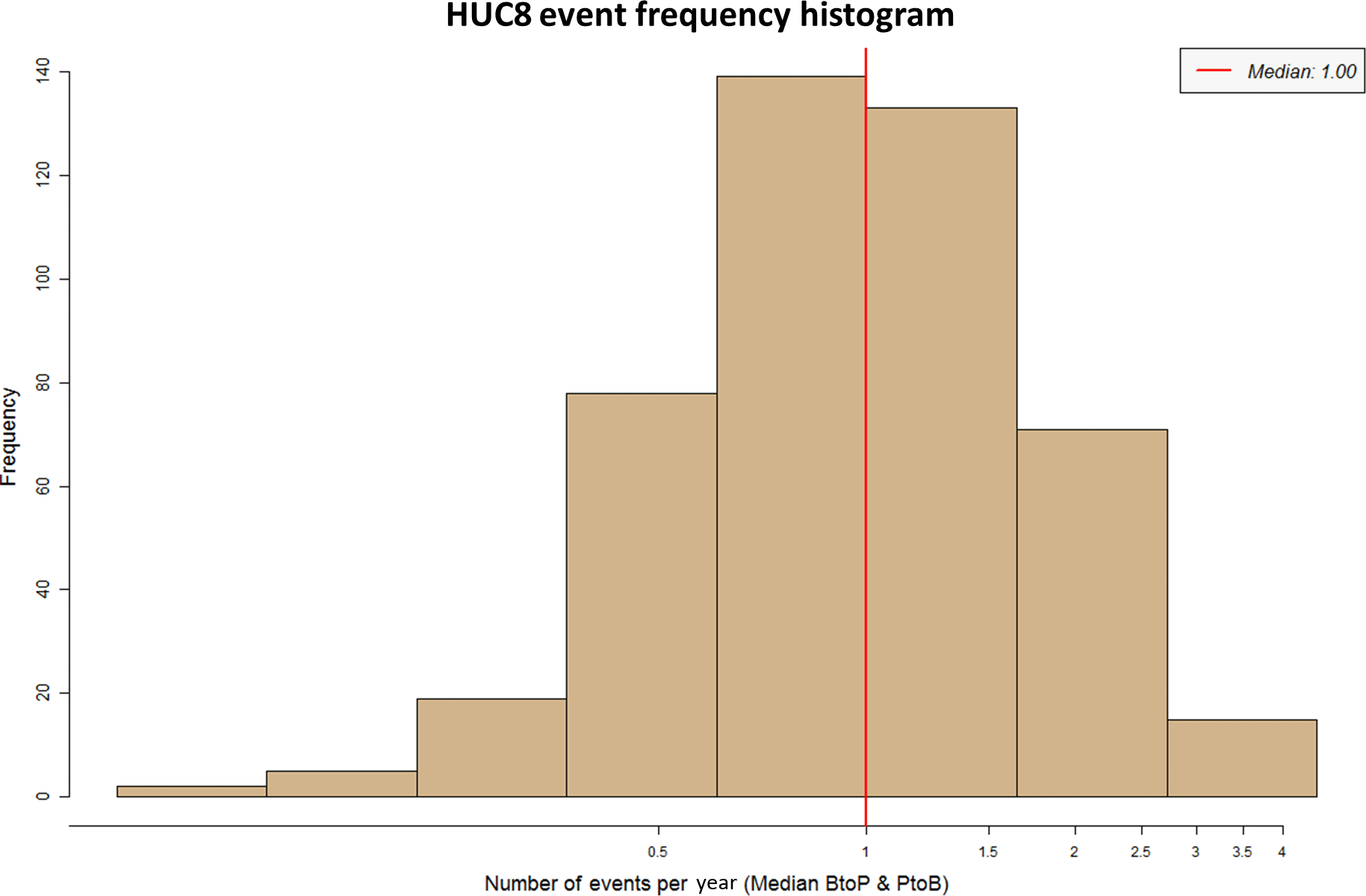
Nationally, the median frequency of events in the HUC8 basins was 1.00 events per year while the mean was 1.14 events per year (Fig. 6). This frequency varied regionally, with some areas experiencing higher frequencies (Fig. 1a). Notable population centers that experience elevated frequencies include the upper Midwest (south of Lake Michigan), southern California and southern Florida. For the HUC6 basins, the median frequency of events was 1.87 events per year with a mean of 2.03 events per year (Fig. 7). Similarly to the HUC8 basins, the frequencies varied regionally with some areas of elevated frequencies (Fig. 1b).
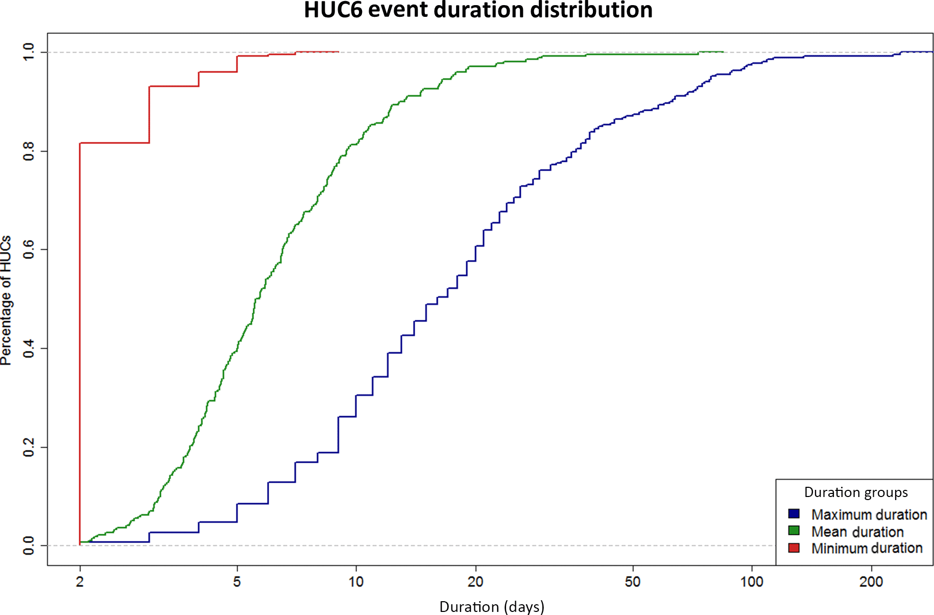
To investigate how event duration varies nationally, we calculate the mean event duration for each basin. Nationally, the mean event duration ranged from 2 to 79 days for the basins defined by the HUC8 and 2 to 73 days for the basins defined by the HUC6. The mean event duration for 95 % of HUC8 and HUC6 basins is less than 14 and 17 days respectively (Figs. 8 and 9). The minimum event duration was 2 days and was observed at 336 HUC8s and 227 HUC6s. The maximum event duration for HUC8s was 232 days and occurred in the 10160003 basin. For HUC6 basins that maximum event duration was 237 days occurring in the 101600 basin. When we look at the shape of both curves, we can see that there is a higher percentage of HUC8s that have shorter mean and maximum durations, as the curves approach the lower event durations more rapidly, leading to a steep curve when compared to the curves for the HUC6. However, when we look at the minimum duration, a larger percentage of the HUC6s have a minimum duration of 2 days when compared to the HUC8, which is an indication that there is a larger number of events that are impacting only one site. While both the HUC6 and the HUC8 taper off towards the higher event durations, there is a lower percentage of the HUC8s that have event durations greater than 20 days. With those two factors we can see that durations within each HUC6 have a wider range than those compared to the HUC8.
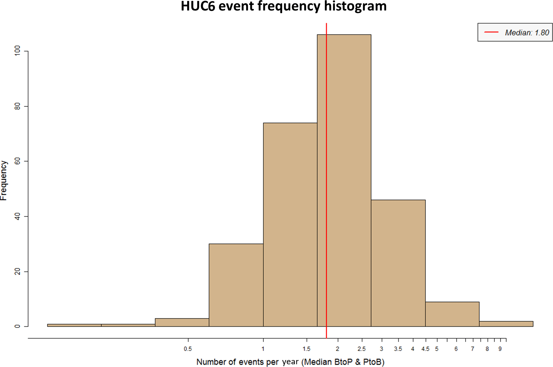
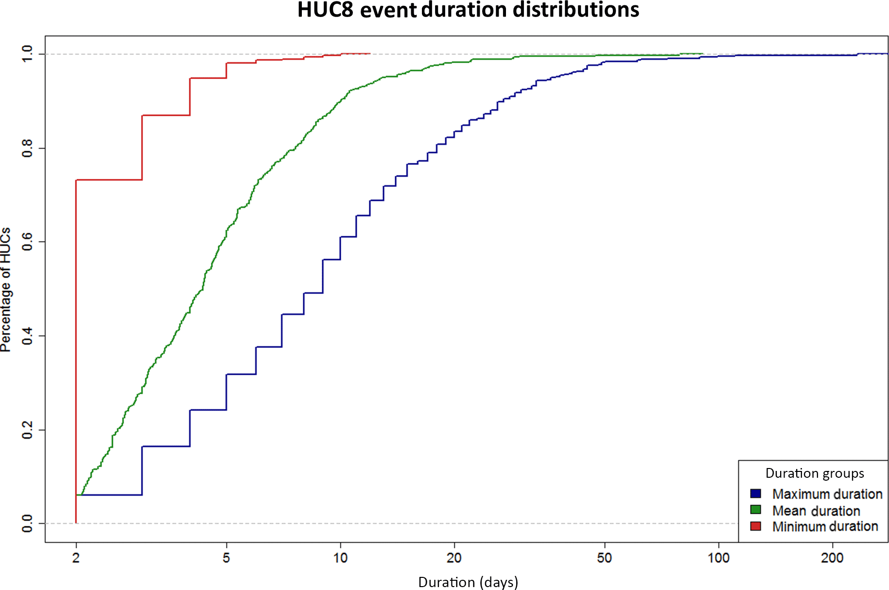
Figure 10 represents two sites that reflect longer recession periods following their peaks. With a data-driven approach identifying the generation and recession of the events, certain extreme events may show increased event durations. The extreme durations are a reflection of the minimum threshold as well as the hydrological processes at hand. Looking at the two sites, the one in Fig. 10a is located in South Dakota and that in Fig. 10b is located in Florida; both of the extreme events that are observed have certain factors that impacted their recessions. The site in South Dakota experienced an event that was impacted by the melting of an ice jam represented by the quick generation. Following the melt there was a significant rain event as well as a release of water from a dam further upstream. The site on the right is located on a natural tourist spring. These springs contain a significant amount of groundwater. Following an intense rain event the buildup of water caused the increased recession. When we define an events' duration as the first occurrence of discharge above the Q2 to the final occurrence of discharge below the Q2, if our site is impacted by a natural occurrence, events will reflect longer-than-expected durations. Further analysis will be conducted to examine changes to the minimum threshold to examine the influence of these natural processes. While a majority of the durations reflect reasonable time frames for flooding events that exceed the Q2, it is important to note that the method might not be appropriate for all streams.

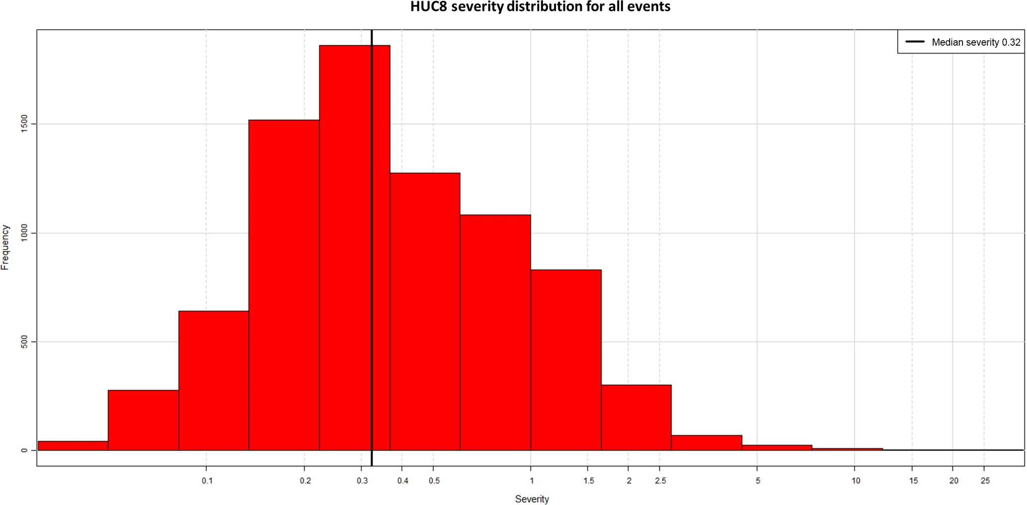
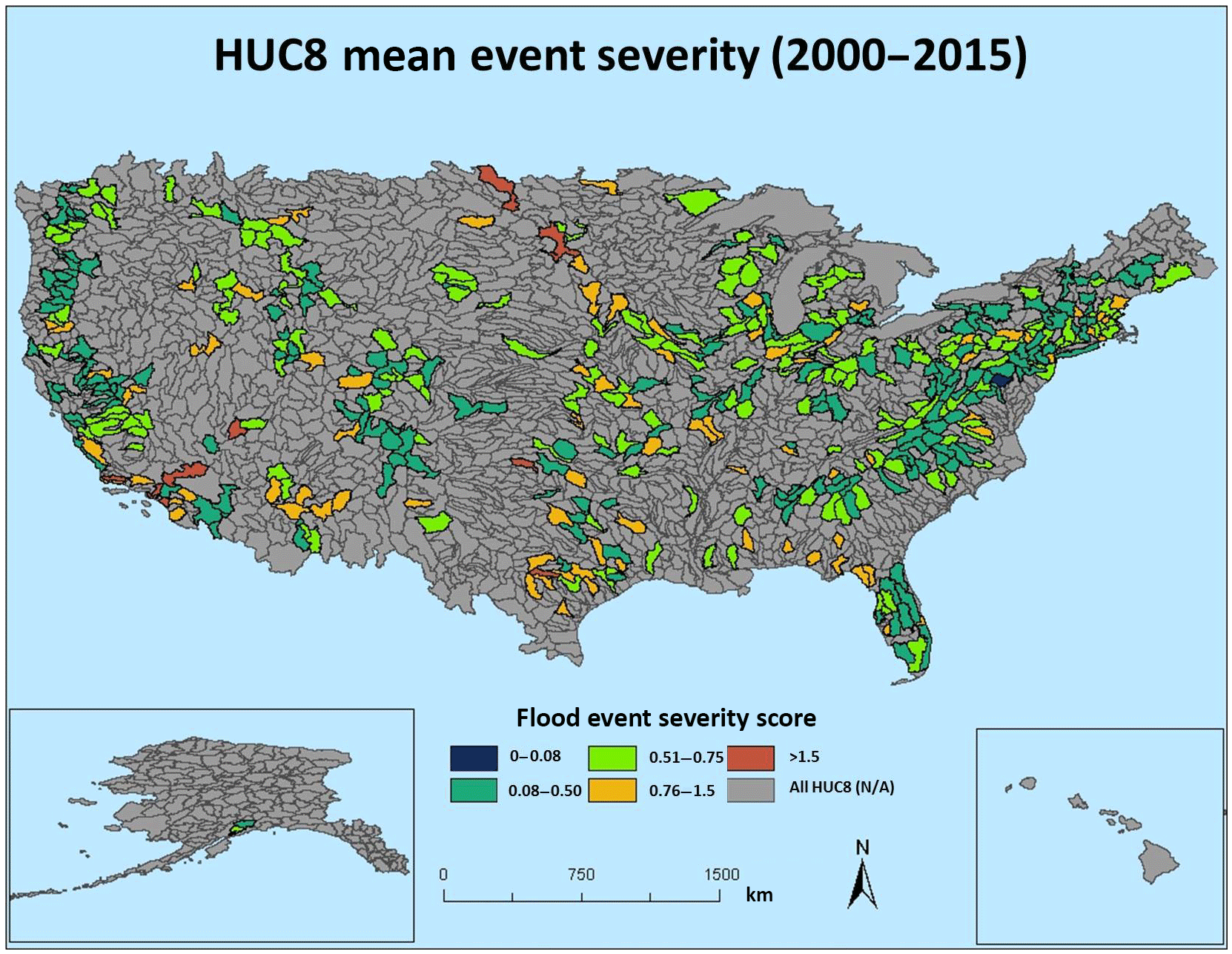
When looking at the distribution of severity scores there is a slight skew towards the extreme events. Severity scores ranged from the least severe (0.032) to the most severe (26.9; Fig. 11), with a median severity score of 0.32 and a mean of 0.57. While the range in severity scores is quite large, a majority of the events received a score less than 1. Regionally the severity scores are generally distributed evenly throughout the country (Fig. 12). There appear to be pockets of higher severities but across the country there does not appear to be a pattern within the regional distribution. While it is evenly distributed regionally, within the regions we can see the wide range in severity that was observed in the distribution of frequency.
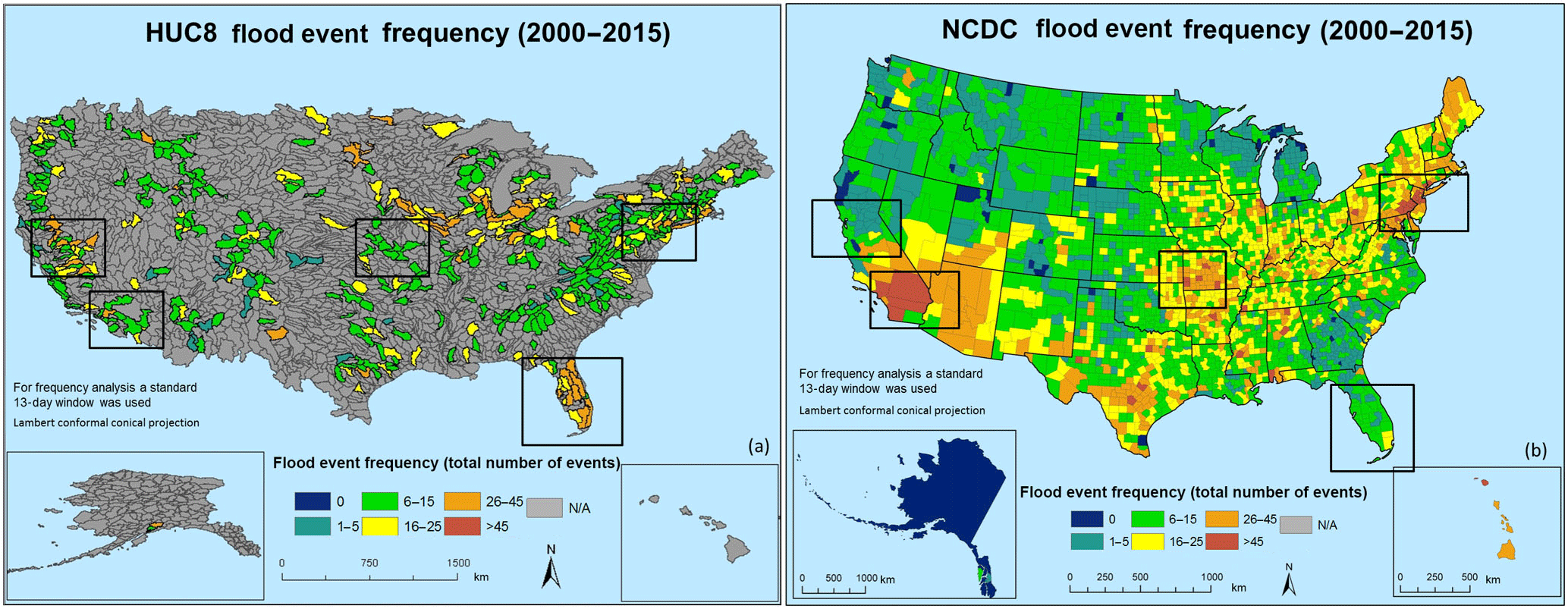
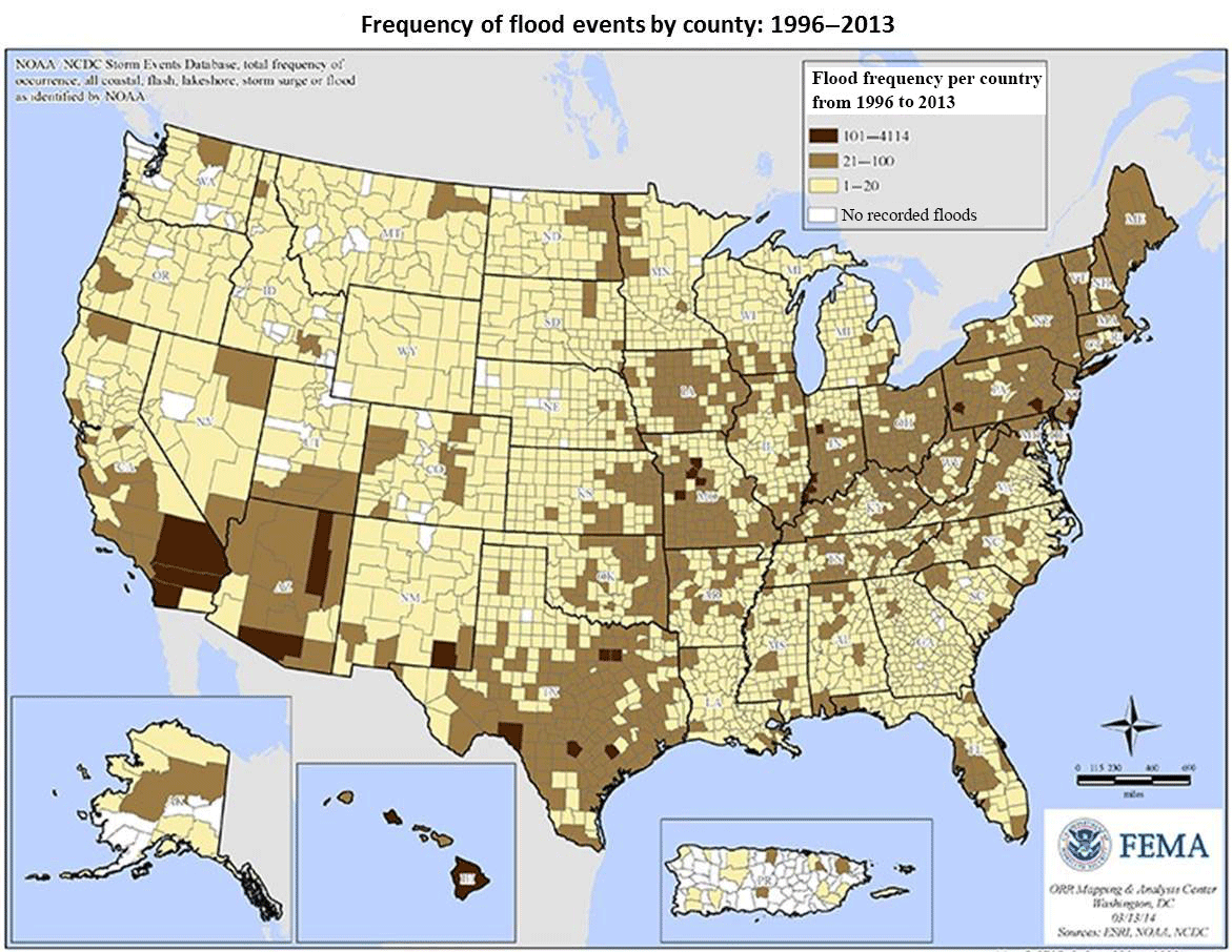
Finally, comparisons were made to other methodologies applied to the same dataset as well as other publically accessible datasets. The first comparison examined a method used by FEMA to estimate floods using NCDC Storm Events Database (Fig. 13) (ORR Mapping and Analysis Center, 2014). The distribution of events was broken down into total event frequency by county ranging from 1 to 4114. While the trained spotters follow guidelines in identifying events, the method lacks a way to group events. The inability to group events that would otherwise be considered a single event leads to an overestimation of events. This overestimation is evident when it is noted that the maximum frequency of events for a specific county was 4114.
The final comparison was made to the NCDC applying a 13-day standard window. While the NCDC map provides a more complete national coverage two patterns occur (Fig. 14). Within the five boxed areas, either the NCDC frequency is far greater or the daily discharge frequency was far greater. For example, in Florida, we see frequency range from 6 to 25 events for NCDC observations but events observed through daily discharge range from 26 to 45. The opposite occurs in Missouri, with NCDC estimates ranging from 16 to 85 events and events observed through daily discharge ranging from 6 to 15.
From these estimates there is no obvious reason for the discrepancies in frequencies but we can speculate. For example Florida experiences significantly fewer events using NCDC data than the daily discharge data. A possible explanation could be how trained spotters define events (National Oceanographic and Atmospheric Administration, 2007). An area in Florida may experience a peak over the threshold triggering our event definition, yet that peak may not be recorded as an NCDC observation based on the spotter's perspective. Another reason could be due to the fact that these trained spotters respond to citizen's reports and, due to the frequency of flooding in an area like Florida, the citizen may not call and the peak may not be recorded.
However a similar thought process can be applied to our threshold selection. As stated the minimum threshold was selected as a representation of bank-full discharge. While this assumption was the basis for our method, in certain areas it is conceivable that the threshold may be lower than bank-full discharge, which could possibly lead to an overestimation of flooding events in certain areas. There is no certain explanation for the discrepancies in the results. With no certain explanation for the results from this comparison, the assumptions that define the compared methodologies will be explored in future analyses.
This study was able to provide a data-driven approach in attempts to solve the issues of inconsistent event definitions within the (re)insurance industry. We derived a methodology based on a peak over threshold analysis that was able to capture and aggregate multiple occurrences of flooding at various locations. Using physical assumptions, our minimum threshold and window of independence were able to capture each individual sites reaction to passing flood waves. An approach identifying windows based on the impacted site allows for each site to represent their individual characteristics of flooding rather than applying standard metrics throughout. Each event was defined through their duration, impacted area and magnitude. The development of a severity index examines overall impacted areas as well as individual flood magnitudes.
Analyses were conducted on both HUC8 and HUC6 to determine which size of Hydrological Unit Code was more applicable for further analysis. 7932 HUC8 and 8444 HUC6 events were identified during our study. Understanding the applicability of different basin sizes is important because it aids in our main goal of applying a consistent definition to reinsurance contracts. From our definition our goal was to understand the frequency that represents an entire basin or area. We also hope to use the definition to define a parametric trigger or an alternative form of defining the event. All of this is possible when we know what basin size is the most applicable. The HUC8 was chosen as a more applicable basin size as it was a better representation of site interaction during flooding events.
Nationally, there are areas with large discrepancies between the HUC6 and HUC8 frequencies. One explanation of this discrepancy is represented by the HUC6 basin 071200 (Fig. 4). The area of this HUC6 is 28 309.78 km2 and contains 6 HUC8s. The annual frequency of events of the HUC8 ranges between 1 and 2.33, while the HUC6 produces 5 events per year. Although it is expected that the larger basin will have a slightly higher frequency due to some events occurring in one part of the basin and not impacting the other, a more than doubling of events per year indicates that a large number of events do not interact with other sites in the basin. This lack of interaction is inconsistent with the goal of this research to identify basin-wide event frequencies. The inconsistencies and lack of interaction are represented by the relationship between site count on frequency.
Based on our analysis of two levels of HUCs, determining which basin size was the most appropriate was a crucial portion of our analysis. To determine which was more appropriate, distributions of the percentage sites impacted were analyzed in order to see how sites were interacting during events. When examining the CDF of the percentage of sites impacted (Fig. 5), we can see that the HUC8 is the more applicable basin level to use for our analysis. HUC8s showed a higher percentage of events and a higher percentage of sites impacted that were impacted during each event when compared to the HUC6. With this comparison we can see that there are more individual events that are being aggregated to basin events rather than those events being segmented into multiple events. With this aggregation we are seeing a more complete picture of frequencies at the HUC8 than the HUC6.
We found that HUC8 frequencies are relatively normally distributed but are unevenly distributed regionally. For all HUC8s a median of 15 events (1 event per year) and mean of 17.21 events (1.14 events per year) were recorded. In a number of areas there were pockets of elevated frequencies. Durations for all events ranged from 2 to 232 days with a mean duration of 6.34 days. The wide range of event durations prompts further investigation into events with durations in the positive tail of the distribution. For example, we considered two HUC8s, one in South Dakota (10160003) and another in Florida (03100207), that are impacted by natural events leading to longer durations. Some sites within these two basins were affected by ice jams as well as natural springs, which have contributed to significant recessions of their events. While these events are natural, the resulting event durations should prompt examination into the selection of thresholds for the sites, as an assumption of bank-full discharge might be slightly lower than a threshold that produces flooding. Investigation into the bank-full discharge assumption is necessary when determining the appropriate level of flooding to conduct our methodology. Analyses will be conducted testing our methodology using varying levels of flooding, comparing our estimates using the Q2 to Q5 and Q10. In addition to testing the various levels of flooding based on return period, we will examine the impact of the estimated bank-full discharge to the observed.
Severity scores calculated for all events in the dataset showed a slight skew toward the more extreme events. The smaller and local events are represented by the median of 0.32 and mean of 0.57, as we can expect events slightly above the threshold to not necessarily affect all the sites in the basin, producing a score less than 1. Regionally severity is relatively evenly distributed nationally.
With a data-driven approach to our methodology, a focus on the individual site parameters shifts the focus from generalities about events to site-specific understanding, leading to an applicable method regionally. A fundamental aspect of this research is to understand spatial extent of flooding and we were able to expand from single gauge stations to entire basins. The data-driven approach allowed us to apply the methodology to a number of basins with varying characteristics. The final advantage to our method is that when looking at flood severity we do not look at magnitude exclusively but the addition of spatial extent adds an element to differences in severity regionally.
While there are a number of advantages that come from this method, relying on public data has revealed drawbacks in its application. Using a data-driven method limits our ability to estimate frequencies in areas that do not have data. Across all USGS gauges there is no uniformity in data availability for a number of years or number of stations within a basin. Through our site selection process we were only able to use 20 % of all available HUC8s, which limits national coverage in our estimates.
The minimum threshold for flooding is based on the assumption that it is a representation of bank-full discharge; in certain areas this may not be accurate. Riverbanks are not uniform, so how bank-full discharge is recognized at each site is dependent on that location, which may lead to underestimation or overestimation of flood stage at that site. The final drawback we observed was that when taking the median of the BtoP and PtoB, slight variations in the event window occurred on the more extreme events. Instead of the median, other statistics will be tested to determine the most applicable way to represent the basin flood generation and recession.
For further research a comparative analysis will be conducted by altering the threshold to examine how that might affect frequency as well as severity. Increasing the time frame will also provide insight into whether or not this 15-year period is representative of the entire time frame of data or if we see a significant increase in events during certain subperiods. Seasonality tests will be run to observe areas more frequently and more severe times of year, which may also provide insight for risk managers. The final test that will need to be conducted is a sensitivity analysis on the threshold selected to prove which threshold is the most reasonable for an analysis such as this.
All calculation and download scripts have been included in the Supplement. All scripts were written using R-Studio.
All data are publically available from the NCDC Storm Events database as well as the USGS stream gauge data sites. A list of sites and a list of the years used will be included as well as the compiled file of the data, added to the Supplement (https://www1.ncdc.noaa.gov/pub/data/swdi/stormevents/csvfiles/, NOAA, 2016; https://waterdata.usgs.gov/nwis/uv, USGS, 2016; https://weather.com/safety/floods/news/flooding-united-states-frequency, Weather Channel, 2016).
Severity score
The supplement related to this article is available online at: https://doi.org/10.5194/hess-22-3761-2018-supplement.
EM and JB designed the methodology. EM wrote and executed code to carry out the methodology. EM wrote the paper with help from JB.
The authors declare that they have no conflict of interest.
The opinions expressed by authors contributing to this journal do not necessarily reflect the opinions of the Hydrology and Earth System Sciences Journal or the institutions with which the authors are affiliated. The data and code used within this research are a property of Guy Carpenter and Co. LLC.
I would like to acknowledge the support of Guy Carpenter LLC and the Nat/Geo
group within the Analytics Department. I would also like to thank my
advisors from the University of Miami, Igor Kamenkovich, David Letson, Roni Avissar
for supporting me during my time at The University of Miami as well as my time
at Guy Carpenter and Company LLC.
Edited by: Bill X. Hu
Reviewed by: three anonymous referees
Bacova-Mitkova, V. and Onderka, M.: Analysis of extreme hydrologicqal events on the Danube using the peak over threshold method, J. Hydrol. Hydromech., 58, 88–101, https://doi.org/10.2478/v10098-010-0009-x, 2010.
Barredo, J. I., Saurí, D., and Llasat, M. C.: Assessing trends in insured losses from floods in Spain 1971–2008, Nat. Hazards Earth Syst. Sci., 12, 1723–1729, https://doi.org/10.5194/nhess-12-1723-2012, 2012.
Black, A. R. and Werritty, A.: Seasonality of flooding: a case study of North Britain, J. Hydrol., 195, 1–25, https://doi.org/10.1016/S0022-1694(96)03264-7, 1997.
Dobour, J. C. and Noel, J.: A climiatological assessment of flood events in Georgia, National Oceanographic and Atmospheric Administration (NOAA), 2005.
Doocy, S., Daniels, A., Murray, S., and Kirsch, T. D.: The Human Impact of Floods: a Historical Review of Events 1980–2009 and Systematic Literature Review, in: PLOS Currents Disasters, 1st Edn., PLOS, https://doi.org/10.1371/currents.dis.f4de, 2013.
FEMA: The National Flood Insurance Program, FEMA.gov., https://www.fema.gov/national-flood-insurance-program (last access: July 2018), 2016.
Gaffin, D. M. and Hotz, D. G.: Precipitation and flood climatology with synoptic features of heavy rainfall accress the Southern Appalachian Mountains, NOAA/National Weather Service, https://www.weather.gov/mrx/heavyrainclimo (last access: July 2018), 2000.
Himmelsbach, I., Glaser, R., Schoenbein, J., Riemann, D., and Martin, B.: Reconstruction of flood events based on documentary data and transnational flood risk analysis of the Upper Rhine and its French and German tributaries since AD 1480, Hydrol. Earth Syst. Sci., 19, 4149–4164, https://doi.org/10.5194/hess-19-4149-2015, 2015.
Joyce, C.: Federal Flood Insurance Program Drowning In Debt. Who Will Pay?, NPR, http://wunc.org/post/federal-flood-insurance-program-drowning-debt-who-will-pay#stream/0 (last access: July 2018), 2014.
Kahana, R., Ziv, B., Enzel, Y., and Dayan, U.: Synoptic climatology of major floods in the Negev Desert, Israel, Int. J. Climatol., 22, 867–882, 2002.
Karnbaum, K. and Dr. Kron, W.: What Is a Flood? Defining Flood Loss Occurrences for Reinsurance Purposes, Munich Re Insurance Company, 2005.
Mallakpour, I. and Villarini, G.: The Changing Nature of Flooding across the Central United States, Nat. Clim. Change, 5.3, 250–254, 2015.
Mallakpour, I. and Villarini, G.: Investigating the relationship between the frequency of flooding over the central United States and large-scale climate, Adv. Water Resour., 92, 159–171, 2016.
National Oceanographic and Atmospheric Administration: National Weather Service Instruction 10-1605, 2007.
Nied, M., Pardowitz, T., Nissen, K., Ulbrich, U., Hundecha, Y., and Merz, B.: On the relationship between hydro-meteorological patterns and flood types, J. Hydrol., 519, 3249–3262, https://doi.org/10.1016/j.jhydrol.2014.09.089, 2014.
NOAA: Index of /pub/data/swdi/stormevents/csvfiles, https://www1.ncdc.noaa.gov/pub/data/swdi/stormevents/csvfiles/, last access: 10 June 2016.
ORR Mapping and Analysis Center: Washington, D.C., ESRI, USGS, 2014.
Uhlemann, S., Thieken, A. H., and Merz, B.: A consistent set of trans-basin floods in Germany between 1952–2002, Hydrol. Earth Syst. Sci., 14, 1277–1295, https://doi.org/10.5194/hess-14-1277-2010, 2010.
Union of Concerned Scientists: Overwhelming Risk: Rethinking Flood Insurance in a World of Rising Seas (2013), https://www.ucsusa.org/global_warming/science_and_impacts/impacts/flood-insurance-sea-level-rise.html#.W0dibdVKjIU (last access: July 2018), 2016.
USGS: Current Conditions for the Nation: Build Time Series, USGS Water Data for the Nation, https://waterdata.usgs.gov/nwis/uv, last access: 10 June 2016.
Weather Channel: Where Flooding Has Been Most Frequent in the U.S., https://weather.com/safety/floods/news/flooding-united-states-frequency, last access: 2 August 2016.