ERA-5 and ERA-Interim driven ISBA land surface model simulations: which one performs better?

The European Centre for Medium-Range Weather Forecasts (ECMWF) recently released the first 7-year segment of its latest atmospheric reanalysis: ERA-5 over the period 2010–2016. ERA-5 has important changes relative to the former ERA-Interim atmospheric reanalysis including higher spatial and temporal resolutions as well as a more recent model and data assimilation system. ERA-5 is foreseen to replace ERA-Interim reanalysis and one of the main goals of this study is to assess whether ERA-5 can enhance the simulation performances with respect to ERA-Interim when it is used to force a land surface model (LSM). To that end, both ERA-5 and ERA-Interim are used to force the ISBA (Interactions between Soil, Biosphere, and Atmosphere) LSM fully coupled with the Total Runoff Integrating Pathways (TRIP) scheme adapted for the CNRM (Centre National de Recherches Météorologiques) continental hydrological system within the SURFEX (SURFace Externalisée) modelling platform of Météo-France. Simulations cover the 2010–2016 period at half a degree spatial resolution.

The ERA-5 impact on ISBA LSM relative to ERA-Interim is evaluated using remote sensing and in situ observations covering a substantial part of the land surface storage and fluxes over the continental US domain. The remote sensing observations include (i) satellite-driven model estimates of land evapotranspiration, (ii) upscaled ground-based observations of gross primary production, (iii) satellite-derived estimates of surface soil moisture and (iv) satellite-derived estimates of leaf area index (LAI). The in situ observations cover (i) soil moisture, (ii) turbulent heat fluxes, (iii) river discharges and (iv) snow depth. ERA-5 leads to a consistent improvement over ERA-Interim as verified by the use of these eight independent observations of different land status and of the model simulations forced by ERA-5 when compared with ERA-Interim. This is particularly evident for the land surface variables linked to the terrestrial hydrological cycle, while variables linked to vegetation are less impacted. Results also indicate that while precipitation provides, to a large extent, improvements in surface fields (e.g. large improvement in the representation of river discharge and snow depth), the other atmospheric variables play an important role, contributing to the overall improvements. These results highlight the importance of enhanced meteorological forcing quality provided by the new ERA-5 reanalysis, which will pave the way for a new generation of land-surface developments and applications.

1 Introduction

Observing and simulating the response of land biophysical variables to extreme events is a major scientific challenge in relation to the adaptation to climate change. To that end, land surface models (LSMs) constrained by high-quality gridded atmospheric variables and coupled with river-routing models are essential (Schellekens et al., 2017; Dirmeyer et al., 2006). Such LSMs should represent land surface biogeophysical variables like surface and root zone soil moisture (SSM and RZSM, respectively), biomass, and leaf area index (LAI) in a way that is fully consistent with the representation of surface and energy flux as well as river discharge simulations. Land surface simulations, such as those from the Global Soil Wetness Project (GSWP, Dirmeyer et al., 2002, 2006; Dirmeyer, 2011), combined with seasonal forecasting systems have been of paramount importance in triggering progress in land-related predictability as documented in the Global Land–Atmosphere Coupling Experiments (GLACE; Koster et al., 2009a, 2011). The land surface state estimates used in those studies were generally obtained with offline (or stand-alone) model simulations, forced by 3-hourly meteorological fields from atmospheric reanalysis. In the past decade, several improved global atmospheric reanalyses of the satellite era (1979–onwards) have been produced that enable new applications of offline land surface simulations. Amongst them are NASA's Modern Era Retrospective Analysis for Research and Applications (MERRA; Rienecker et al., 2011, and MERRA2; Gelaro et al., 2017) as well as ECMWF's (European Centre for Medium-Range Weather Forecasts) Interim reanalysis (ERA-Interim; Dee et al., 2011). Their offline use in either LSMs or land data assimilation system (LDAS), with or without meteorological corrections (e.g. precipitations), led to global land surface variables (LSVs) reanalysis data sets that can support, for example water resources analysis (Schellekens et al., 2017), like MERRA-Land and MERRA2-Land (Reichle et al., 2011, 2017), ERA-Interim/Land (Balsamo et al., 2015), the forthcoming ERA5-Land (Muñoz-Sabater et al., 2018), the North American LDAS (NLDAS; Mitchell et al., 2004), the Global LDAS (GLDAS; Rodell et al., 2004) and LDAS-Monde (Albergel et al., 2017). The quality of those offline land surface simulations relies on the accuracy of the forcing and of the realism of the LSM itself (Balsamo et al., 2015).

ECMWF recently released the first 7-year segment of its latest atmospheric reanalysis: ERA-5 over the period 2010–2016. ERA-5 has important changes relative to the former ERA-Interim atmospheric reanalysis including higher spatial and temporal resolutions as well as a better global balance of precipitation and evaporation. As ERA-5 will eventually replace the ERA-Interim reanalysis assessing its ability to force a LSM with respect to ERA-Interim is highly relevant. In this study, ERA-5, ERA-Interim and a combination of both (ERA-5 with precipitation of ERA-Interim) are used to constrain the CO₂-responsive version of the Interactions between Soil, Biosphere, and Atmosphere (ISBA; Noilhan and Mahfouf, 1996; Calvet et al., 1998, 2004; Gibelin et al., 2006) LSM fully coupled with the CNRM (Centre National de Recherches Météorologiques) version of the Total Runoff Integrating Pathways (TRIP; Oki et al., 1998) continental hydrological system (CTRIP hereafter; Decharme et al., 2010) within the SURFEX (SURFace Externalisée; Masson et al., 2013) modelling system of Météo-France. The ISBA models leaf-scale physiological processes and plant growth, with transfer of water and heat through the soil relying on a multilayer diffusion scheme.

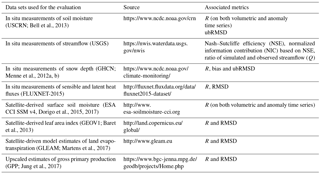
In this study, SURFEX is applied over a data-rich area: North America (latitudes from 20.0 to 55.0^∘ N, longitudes from 130.0 to 60.0^∘ W) for the period 2010–2016. ERA-5 added values with respect to ERA-Interim are assessed by providing verification and diagnostics comparing ISBA LSV outputs when forced by either ERA-5, ERA-Interim, ERA-5 with ERA-Interim precipitations to several in situ measurement data sets or satellite-derived estimates of Earth observations. Specifically, in situ measurements of (i) soil moisture from the USCRN (US Climate Reference Network; Bell et al., 2013) spanning the United States of America and (ii) turbulent heat fluxes from FLUXNET-2015 (http://fluxnet.fluxdata.org/data/fluxnet2015-dataset/, last access: June 2018) are used in the evaluation, together with (iii) river discharges from the United States Geophysical Survey (USGS; https://waterwatch.usgs.gov/, last access: June 2018) and (iv) snow depth measurements from the Global Historical Climatology Network (GHCN; Menne et al., 2012a, b). The following are also used: (i) satellite-driven model estimates of land evapotranspiration from the Global Land Evaporation Amsterdam Model (GLEAM; Martens et al., 2017), (ii) upscaled ground-based observations of gross primary production (GPP) from the FLUXCOM project (Jung et al., 2017), (iii) satellite-derived estimates of surface soil moisture (SSM) from the Climate Change Initiative (CCI) of the European Space Agency (ESA CCI SSM v4; Dorigo et al., 2015, 2017) and (iv) satellite-derived estimates of LAI from the Copernicus Global Land Service program (CGLS; http://land.copernicus.eu/global/, last access: June 2018).

Section 2 presents the details of two atmospheric reanalyses data sets (ERA-Interim and ERA-5), the SURFEX model configuration and the evaluation strategy with the observational data sets. Section 3 provides a set of statistical diagnostics to assess and evaluate the impact of ERA-5 on ISBA with respect to ERA-Interim. Finally, Sect. 4 provides perspectives and future research directions.

2 Methodology

2.1 ERA-Interim and ERA-5 reanalyses

ERA-Interim is a global atmospheric reanalysis produced by ECMWF (Dee et al., 2011). It uses the integrated forecast system (IFS) version 31r1 (more information at https://www.ecmwf.int/en/forecasts/documentation-and-support/changes-ecmwf-model/ifs-documentation, last access: June 2018) with a spatial resolution of about 80 km (T255) and with analyses available for 00:00, 06:00, 12:00 and 18:00 UTC. It covers the period from 1 January 1979 onward and continues to be extended forward in near-real time (with a delay of approximately 1 month). Reanalyses merge observations and model forecasts in data assimilation methods to provide an accurate and reliable description of the climate over the last few decades. Berrisford et al. (2009) provide a detailed description of the ERA-Interim product archive. ERA-5 (Hersbach and Dee, 2016) is the latest and fifth generation of European reanalyses produced by the ECMWF and a key element of the EU-funded Copernicus Climate Change Service (C3S). It is expected that ERA-5 will replace the production of the current ERA-Interim reanalysis (Dee et al., 2011) before the end of 2018, from 1979 to close to the Near Real Time (NRT) period, i.e. in ERA-5 regular routine updates will be conducted to keep close to NRT. In a second phase, an extension back to 1950 is also expected. ERA-5 adds different characteristics to ERA-Interim reanalysis, which makes it richer in term of climate information.

ERA-5 uses one of the most recent versions of the Earth system model and data assimilation methods applied at ECMWF, which makes it able to use modern parameterizations of Earth processes compared to older versions used in ERA-Interim. For instance, developments were done at ECMWF which allows the reanalysis to use a variational bias scheme not only for satellite observations but also for ozone, aircraft and surface pressure data. ERA-5 also benefits from reprocessed data sets that were not ready yet during the production of ERA-Interim. Two other important features of ERA-5 are the improved temporal and spatial resolutions: from 6-hourly in ERA-Interim to hourly in ERA-5, and from 79 km in the horizontal dimension and 60 levels in the vertical to 31 km and 137 levels in ERA-5. Finally, ERA-5 also provides an estimate of uncertainty through the use of a 10-member ensemble of data assimilations (EDA) at a coarser resolution (63 km horizontal resolution) and 3-hourly frequency.

2.2 SURFEX modelling system

2.2.1 The ISBA land surface model

This study makes use of the CO₂-responsive version of the ISBA LSM included in the open-access SURFEX modelling platform of Météo-France (Masson et al., 2013). The most recent version of SURFEX (version 8.1) is used with the “NIT” biomass option for ISBA. The latter simulates the diurnal cycle of water and carbon fluxes, plant growth, and key vegetation variables like LAI and above-ground biomass on a daily basis. It can be coupled to the CTRIP river-routing model in order to simulate streamflow. In this version of ISBA, a single-source energy budget of a soil–vegetation composite is computed. Also, the ISBA parameters are defined for 12 generic land surface patches, which include nine plant functional types (needle leaf trees, evergreen broadleaf trees, deciduous broadleaf trees, C₃ crops, C₄ crops, C₄ irrigated crops, herbaceous, tropical herbaceous and wetlands), bare soil, rocks, and permanent snow and ice surfaces. A more comprehensive model description can be found in Masson et al. (2013).

ISBA accounts for the atmospheric CO₂ concentration on stomatal aperture (Calvet et al., 1998, 2004; Gibelin et al., 2006). Also, photosynthesis and its coupling with stomatal conductance on a leaf level are accounted for. The vegetation net assimilation of CO₂ is estimated and used as an input to a simple vegetation growth submodel able to predict LAI: photosynthesis drives the dynamic evolution of the vegetation biomass and LAI variables in response to atmospheric and climate conditions. During the growing phase, enhanced photosynthesis corresponds to a CO₂ uptake, which leads to vegetation growth. In contrast, lack of photosynthesis leads to higher mortality rates. The GPP is defined as the carbon uptake while the ecosystem respiration (RECO) is the release of CO₂, the difference between these two quantities being the net ecosystem CO₂ exchange (NEE). Evaporation due to (i) plant transpiration, (ii) liquid water intercepted by leaves, (iii) liquid water contained in top soil layers and (iv) the sublimation of snow and soil ice are combined to represent the total evaporative flux.

The ISBA 12-layer explicit snow scheme (Boon and Etchevers, 2001; Decharme et al., 2016) and its multilayer soil diffusion scheme (ISBA-Dif) are used. The later is based on the mixed form of the Richards equation (Richards, 1931) and explicitly solves the one-dimensional Fourier law. It also incorporates soil freezing processes developed by Boone et al. (2000) and Decharme et al. (2013). The total soil profile is vertically discretized; both the temperature and moisture of each soil layer are computed according to their textural and hydrological characteristics. The Brookes and Corey model (Brooks and Corey, 1966) determines the closed-form equations between the soil moisture and the soil hydrodynamic parameters, including the hydraulic conductivity and the soil matrix potential (Decharme et al., 2013). The default discretization with 14 layers over 12 m depth is used. The lower boundary of each layer being: 0.01, 0.04, 0.1, 0.2, 0.4, 0.6, 0.8, 1, 1.5, 2, 3, 5, 8 and 12 m deep (see Fig. 1 of Decharme et al., 2011). Amounts of clay, sand and organic carbon in the soil determine the thermal and hydrodynamic soil properties (Decharme et al., 2016). They are taken from the Harmonized World Soil Database (HWSD; Wieder et al., 2014). As for hydrology, the infiltration, surface evaporation and total runoff are accounted for in the soil water balance. The infiltration rate defines the discrepancy between the surface runoff and the throughfall rate. The later being defined as the sum of rainfall not intercepted by the canopy, dripping from the canopy (i.e. interception reservoir) and snow melt water. The soil evaporation affects only the superficial layer (top 1 cm) and is proportional to its relative humidity. Transpiration water from the root zone (the region where the roots are asymptotically distributed) follows the equations in Jackson et al. (1996). Canal et al. (2014) provide more information on the root density profile.

Both the surface runoff (the lateral subsurface flow in the topsoil) and a free drainage condition at the bottom soil layer contribute to ISBA total runoff. The Dunne runoff (i.e. when no further soil moisture storage is available) and lateral subsurface flow from a subgrid distribution of the topography are computed using a basic TOPMODEL approach. The Horton runoff (i.e. when rainfall has exceeded infiltration capacity) is estimated from the maximum soil infiltration capacity and a subgrid exponential distribution of the rainfall intensity.

2.2.2 The CTRIP hydrological system

CTRIP is driven by three prognostic equations corresponding to (i) the groundwater, (ii) the surface stream water and (iii) the seasonal floodplains. Streamflow velocity is computed using the Manning formula as described in Decharme et al. (2010). When the river water level overtops the river-bank, it fills up the floodplain reservoir which empties when the water level drops below this threshold (Decharme et al., 2012). Occurrence of flooding impacts the ISBA soil hydrology through infiltration, and it also influences the overlying atmosphere via free surface-water evaporation and precipitation interception. The groundwater scheme is based on the two-dimensional groundwater flow equation for the piezometric head (Vergnes and Decharme, 2012). Its coupling with ISBA enables accounting for the presence of a water table under the soil moisture column. It allows for upward capillary fluxes into the soil (Vergnes et al., 2014). CTRIP is coupled to ISBA through OASIS-MCT (Voldoire et al., 2017). Once a day, ISBA provides CTRIP with updates on runoff, drainage, groundwater and floodplain recharges, and CTRIP feedbacks to ISBA the water table fall or rise, floodplain fraction, and flood potential infiltration. The current CTRIP version consists of a global streamflow network at 0.5^∘ × 0.5^∘ spatial resolution.

2.3 Evaluation strategy and data sets

Three experiments are considered for the evaluation: (i) SURFEX forced by ERA-Interim, all atmospheric variables interpolated to 0.5^∘ × 0.5^∘ spatial resolution (referred as ei_S hereafter, the benchmark experiment); (ii) SURFEX forced by ERA-5, all atmospheric variables interpolated at 0.5^∘ × 0.5^∘ spatial resolution except precipitation (rain and snow interpolated to hourly time steps assuming a constant flux) that comes from ERA-Interim (referred as e5ei_S hereafter); and (iii) SURFEX forced by ERA-5, all atmospheric variables interpolated at 0.5^∘ × 0.5^∘ spatial resolution (referred as e5_S hereafter). A bilinear interpolation from the native reanalysis grid to the regular grid has been used. For all three experiments, the first year (2010) was spun up 20 times to allow the model to reach equilibrium. Comparing e5_S to ei_S provides the overall improvements from ERA-Interim to ERA-5. The idealized e5ei_S simulation was carried out to assess the role of precipitation changes from ERA-Interim to ERA-5.

This study makes use of several in situ measurement data sets as well as satellite-derived estimates of Earth observations that are described in the next two sections. The different performance metrics used for the evaluation are also described. Their choice is of crucial interest; it is governed by the nature of the variable itself and is influenced by the purpose of the investigation and its sensitivity to the considered variables (Stanski et al., 1989). No single metric or statistic can capture all the attributes of environmental variables; some are robust with respect to some attributes while insensitive to others (Entekhabi et al., 2010). While performance metrics like the correlation coefficient (R), unbiased root mean squared differences (ubRMSD), root mean squared differences (RMSDs) and efficiency score (depending on the considered variable) are first applied to the three simulations independently, metrics like the normalized information contribution (NIC; e.g. Kumar et al., 2009) are then used to quantify improvement or degradation from one data set to another. Table 1 summarizes the different data sets used for the evaluation and the performance metrics used.

Table 1 Evaluation data sets and associated metrics used in this study.

2.3.1 In situ measurement of soil moisture, river discharges, snow depth and fluxes

USCRN is a network of climate-monitoring stations maintained and operated by the National Oceanic and Atmospheric Administration (NOAA). It aims at providing climate-science-quality measurements of air temperature and precipitation. To increase the network's capability of monitoring soil processes and drought, soil observations were added to USCRN instrumentation. At each USCRN station in the conterminous United States in 2011, the USCRN team completed the installation of triplicate-configuration soil moisture and soil temperature probes at five standard depths (5, 10, 20, 50 and 100 cm) as prescribed by the World Meteorological Organization. The 111 stations present data between 2009 and 2016. Stations provide data at an hourly time step. Similar to a prior study, data sets potentially affected by frozen conditions were masked out using an observed temperature threshold of 4 ^∘C (e.g. Albergel et al., 2013a). The second layer of soil of ISBA between 1 and 4 cm depth (the diffusion scheme is used in this study) is compared to in situ measurements at 5 cm depth at a 3-hourly time step (model output) between April and September in order to avoid frozen conditions as much as possible . The ability of ei_S, e5ei_S and e5_S to reproduce surface soil moisture variability is first assessed using the correlation coefficient (R) and unbiased root mean square differences (ubRMSD). Climatology differences between model and in situ observations make a direct comparison difficult (Koster et al., 2009b). Soil moisture time series usually show a strong seasonal pattern possibly increasing the skill values between modelled and observed data sets. To avoid seasonal effects, monthly anomaly time series are calculated. At each grid and observation point, the difference from the mean is produced for a sliding window of 5 weeks, and the difference is scaled to the standard deviation as in Albergel et al. (2013b). For each surface soil moisture estimate at day i, a period F is defined, with $F=[i-\mathrm{17},i+\mathrm{17}]$ (corresponding to a 5-week window). If at least five measurements are available in this period, the average soil moisture value and the standard deviation are calculated. Anomaly time series reflect the time-integrated impact of antecedent meteorological forcing. The latter is mainly reflected in the upper layer of soil. The correlation coefficient is also computed for anomaly time series (R_ano). For correlations, the p value (a measure of the correlation significance) is also calculated indicating the significance of the test (as in Albergel et al., 2010), and only cases where the p value is below 0.05 (i.e. the correlation is not a coincidence) are retained. Stations with nonsignificant R values can be considered suspect and are excluded from the computation of the network average metrics. This process may remove some reliable stations too (e.g. in areas where the model might not realistically represent soil moisture).

Over the period 2010–2016, river discharge from ei_S, e5ei_S and e5_S are compared to daily streamflow data from the USGS http://nwis.waterdata.usgs.gov/nwis, last access: June 2018). Data are chosen for subbasins with large drainage areas (10 000 km² or greater) and with a long observation time series (4 years or more). Smaller basins are excluded due to the low resolution of CTRIP (0.5^∘ × 0.5^∘). It is common to express observed and simulated river discharge (Q) data in m³ s⁻¹. Given that the observed drainage areas may differ slightly from the simulated ones, specific discharge in mm d⁻¹ (the ratio of Q to the drainage area) is used in this study, similarly to Albergel et al. (2017). Stations with drainage areas differing by more than 20 % from the simulated ones are also discarded. This criterion aims to ensure a meaningful comparison between observed and simulated values. It is necessary for coping with the significant distortions in the model representation of the river network that are caused by the coarse spatial resolution of the CTRIP global river network (0.5^∘ × 0.5^∘). Impact on Q is evaluated using the efficiency score (NSE; Nash and Sutcliffe, 1970). NSE evaluates the model ability to represent the monthly discharge dynamics and is given by

$$\begin{array}{}\text{(1)}& \text{NSE}=\mathrm{1}-{\displaystyle \frac{\sum _{t=\mathrm{1}}^T{\left(Q_{\text{s}}^t-Q_{\text{o}}^t\right)}^{\mathrm{2}}}{\sum _{t=\mathrm{1}}^T{\left(Q_{\text{o}}^t-\stackrel{\mathrm{‾}}{Q_{\text{o}}^t}\right)}^{\mathrm{2}}}},\end{array}$$

where $Q_{\text{s}}^t$ is the simulated river discharge (by either ei_S, e5ei_S or e5_S) at time t and $Q_{\text{o}}^t$ is observed river discharge at time t, T is the total number of days and $\stackrel{\mathrm{‾}}{Q_{\text{o}}^t}$ is the average observed discharge. NSE can vary between −∞ and 1. A value of 1 corresponds to identical model predictions and observed data. A value of 0 implies that the model predictions have the same accuracy as the mean of the observed data. Negative values indicate that the observed mean is a more accurate predictor than the model simulation. Only stations with a NSE greater than −1 for the benchmark experiment, ei_S, are considered, leading to 172 stations over the considered domain. A normalized information contribution (NIC; as in Kumar et al., 2009) measure is then computed to quantify the improvement or degradation due to the specific atmospheric reanalysis used to force ISBA. The NIC_NSE values are computed for both e5_S and e5ei_S with respect to ei_S as

$$\begin{array}{}\text{(2)}& {\text{NIC}}_{\text{NSE(e5;5ei)}}={\displaystyle \frac{{\text{NSE}}_{\text{(e5;e5ei)}}-{\text{NSE}}_{\text{(ei)}}}{\mathrm{1}-{\text{NSE}}_{\text{(ei)}}}}.\end{array}$$

The NIC_NSE metric provides a normalized measure of the improvement through the use of either NSE_e5ei or NSE_e5 as a fraction of the maximum possible skill improvement (1−NSE_ei). Positive and negative NIC_NSE values indicate improvements and degradations in either e5_S or e5ei_S relative to ei_S river discharge estimates, respectively. NICs along with their 95 % confidence interval of the median derived from a 10 000 samples bootstrapping are provided for e5_S and e5ei_S. The ratio of simulated and observed river discharges is also computed $\left(Q_{\text{s}}^t/Q_{\text{o}}^t\right)$; the closer to 1 it is, the better the simulated river discharges are.

The Global Historical Climatology Network (GHCN) daily data set, developed to meet the needs of climate analysis and monitoring studies that require data at a daily time resolution, contains records from over 75 000 stations in 179 countries and territories (Menne et al., 2012a, b). Numerous daily variables are provided, including maximum and minimum temperature, total daily precipitation, snowfall and snow depth. In this study, over North America, stations with daily snow depth data from 2010 to 2016, with less than 10 % missing and at least 15 days of snow presences per year on average (to avoid using stations always reporting zero snow depth) are used, it results in 1901 stations out of 2056. The ability of ei_S, e5ei_S and e5_S to reproduce snow depth and its variability is assessed using the bias, correlation coefficient (R) and unbiased root mean square difference (ubRMSD).

Daily observations of sensible and latent heat fluxes from the FLUXNET-2015 data set with at least 2 years of data are used over the period 2010–2016 to evaluate the ability of e5_S, e5ei_S and ei_S to reproduce flux variability. The FLUXNET-2015 data set includes data collected at sites from multiple regional flux networks as well as several improvements to the data quality control protocols and the data processing pipeline (http://fluxnet.fluxdata.org/data/fluxnet2015-dataset/). The 37 stations are retained for the evaluations and two metrics are considered: R and RMSD.

Performance metrics are applied to each individual station of each network; thereafter, network metrics are computed by providing the median values of the statistics from the individual stations within each network. For each metric, the 95 % confidence interval of the median derived from a 10 000 samples bootstrapping is provided.

2.3.2 Satellite-derived estimates of surface soil moisture, leaf area index, land evapotranspiration and gross primary production

In response to the GCOS (Global Climate Observing System) endorsement of soil moisture as an essential climate variable, the European Space Agency Water Cycle Multimission Observation Strategy (WACMOS) project and Climate Change Initiative (CCI; http://www.esa-soilmoisture-cci.org, last access: June 2018) have supported the generation of a surface soil moisture product based on multiple microwave sources (ESA CCI SSM hereafter). The first version of the combined product was released in June 2012 by the Vienna University of Technology (Liu et al., 2011, 2012; Wagner et al., 2012). Several authors (e.g. Albergel et al., 2013a, b; Dorigo et al., 2015, 2017) have highlighted the quality and stability over time of the product. Despite some limitations, this data set has already shown potential in assessing model performance (e.g. Szczypta et al., 2014; van der Schrier et al., 2013). In this study the combined ESA CCI SSM latest version of the product (v4) is used. It merges SSM observations from seven microwave radiometers (SMMR, SSM/I, TMI, ASMR-E, WindSat, AMSR2, SMOS) and four scatterometers (ERS-1, 2 AMI, MetOp-A and B ASCAT) into a combined data set covering the period November 1978 to December 2016. Data are in volumetric (m³ m⁻³) units and quality flags (snow coverage, temperature below 0^∘C or dense vegetation) are provided. For a more comprehensive overview of the product, see Dorigo et al. (2015, 2017). As topographic relief is known to negatively affect remote sensing estimates of soil moisture (Mätzler and Standley, 2000), the time series for pixels whose average altitude exceeded 1500 m above sea level were discarded. Data on pixels with urban land cover fractions larger than 15 % were also discarded, to limit the effects of artificial surfaces. The altitude and urban area thresholds were set according to Draper et al. (2011) and Barbu et al. (2014), who processed satellite-based SSM retrievals for data assimilation studies with the ISBA LSM. As for in situ measurements of soil moisture, correlation is applied to both the volumetric and anomaly time series.

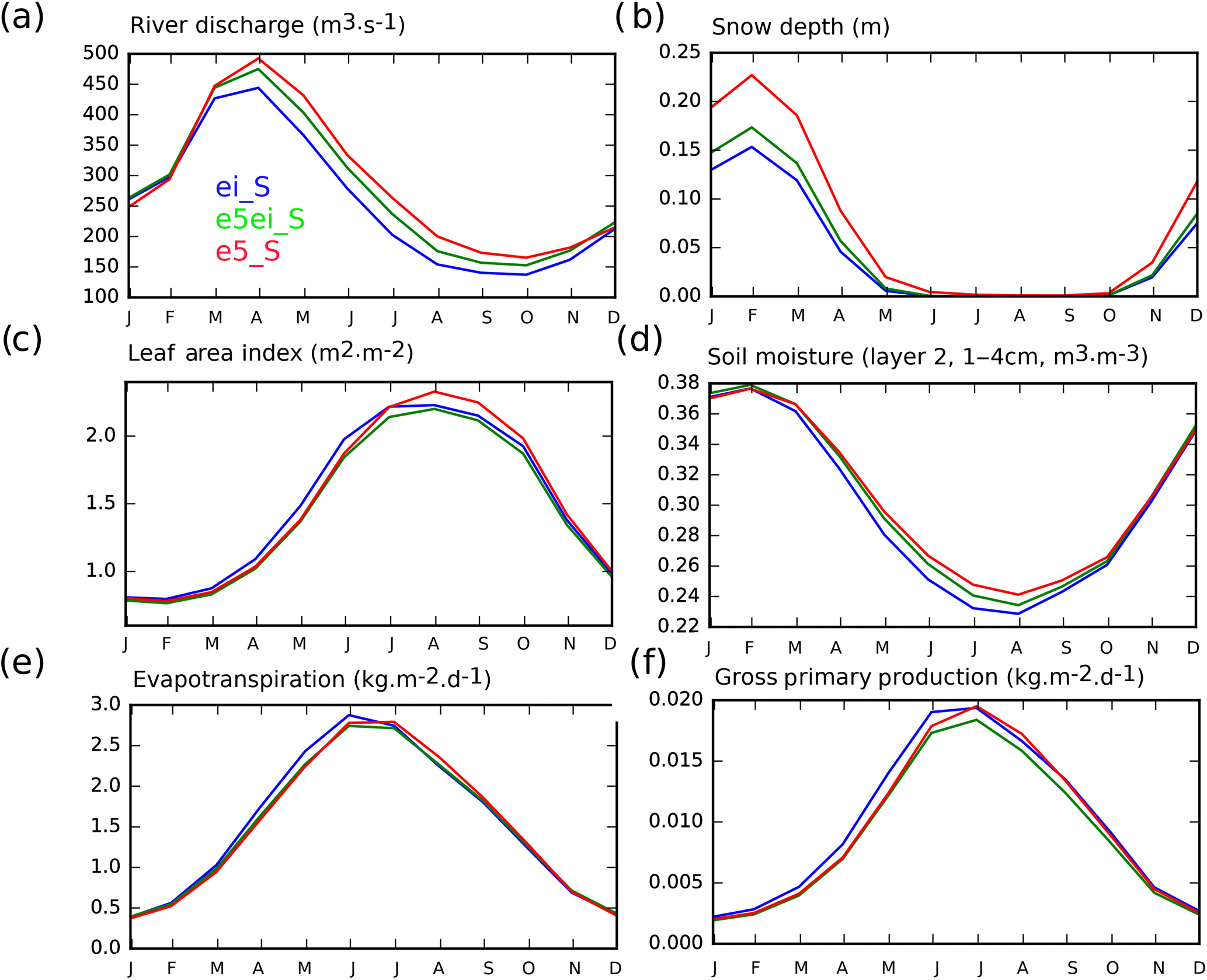
Figure 1 Seasonal time series of the six main land surface variables (LSVs) evaluated in this study over the whole domain for 2010–2016: (a) river discharge, (b) snow depth, (c) leaf area index, (d) liquid soil moisture in the second layer of soil (1–4 cm depth), (e) evapotranspiration and (f) gross primary production. LSVs simulated with SURFEX forced by ERA-Interim (ei_S) are in blue, by ERA-5 (e5_S) with precipitation from ERA-Interim (e5ei_S) in green and by ERA-5 (e5_S) in red.

The GEOV1 LAI used in this study is produced by the European CGLS (http://land.copernicus.eu/global/) as evaluated in Boussetta et al. (2015). The LAI observations are retrieved from the SPOT-VGT and then PROBA-V (from 1999 to present) satellite data according to the methodology proposed by Baret et al. (2013). As in Barbu et al. (2014), the 1 km spatial resolution observations are interpolated by an arithmetic average to the 0.5^∘ model grid points, if at least 50 % of the observation grid points are observed (i.e. half the maximum amount). LAI observations have a temporal frequency of 10 days at best (in presence of clouds, no observations are available). Correlation and root mean squared differences are used to assess the ability of ei_S, e5ei_S and e5_S to reproduce LAI variability.

The GLEAM product uses a set of algorithms to estimate both terrestrial evaporation and RZSM based on satellite data (Miralles et al., 2011). It is a useful validation tool to assess model performance given that such quantities are difficult to measure directly on large scales. Potential evaporation rates are constrained by satellite-derived SSM data, while the global evaporation model in GLEAM is mainly driven by various microwave remote-sensing observations. It is now a well established data set that has been widely used to study land–atmosphere feedbacks (e.g. Miralles et al., 2014b; Guillod et al., 2015), as well as trends and spatial variability in the hydrological cycle (e.g. Jasechko et al., 2013; Greve et al., 2014; Miralles et al., 2014a; Zhang et al., 2016). This study makes use of the latest version available, v4.0. It is a 37-year data set spanning from 1980 to 2016 and is derived from a variety of sources, such as vegetation optical depth and snow water equivalent, satellite-derived SSM estimates, reanalysis air temperature and radiation, and a multi-source precipitation product (Martens et al., 2017). It is available at a spatial resolution of 0.25^∘ × 0.25^∘. A full description of the data set, including an extensive validation using measurements from 64 eddy-covariance towers worldwide is provided by Martens et al. (2017). As for LAI, the correlation and root mean squared differences are the two performance metrics used to evaluate the representation of evapotranspiration from the three data sets.

The final product used in this study is a daily GPP estimate from the FLUXCOM project (Jung et al., 2017). It is an upscaled product derived from the FLUXNET. In FLUXCOM, selected machine-learning-based regression tools that span the full range of commonly applied algorithms (from model tree ensembles to multiple adaptive regression splines, to artificial neural networks, and to kernel methods), and several representatives of each family are used to provide a spatial upscaling of GPP at regional to global scales. It is limited to a 0.5^∘ × 0.5^∘ spatial resolution and a daily temporal resolution over the period 1982–2013 (Tramontana et al., 2016). FLUXCOM fluxes can be used as a way of benchmarking LSMs on large scales (Jung et al., 2009, 2010, 2011; Beer et al., 2010; Bonan et al., 2011; Slevin et al., 2017). The product can be found at the Max Planck Institute for Biogeochemistry data portal (https://www.bgc-jena.mpg.de/geodb/projects/Home.php, last access: June 2018). Correlation and root mean squared differences are the two performance metrics used to evaluate the representation of carbon uptake from the three data sets.

Table 2 Comparison of surface soil moisture with in situ observations for ei_S, e5ei_S and e5_S over the period 2010–2016 (April to September months are considered). Median correlations R (on volumetric and anomaly time series) and ubRMSD are given for the USCRN. Scores are given for significant correlations with p values < 0.05.

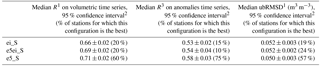
¹ Only for stations presenting significant R values on volumetric time series (p value < 0.05): 110 stations; ² 95% confidence interval of the median derived from a 10 000 samples bootstrapping; ³ Only for stations presenting significant R values on anomaly time series (p value < 0.05): 107 stations

Figure 2 Maps of correlation (R) on volumetric time series (a) and anomaly time series (b) between in situ measurements at 5 cm depth from the USCRN and the ISBA LSM within the SURFEX modelling platform forced by either ERA-Interim (ei_S), ERA-5 with ERA-Interim precipitations (e5ei_S) or ERA-5 (e5_S). For each station presenting significant R (p values < 0.05), the simulation that presents the better R values is represented. Star symbols are when ei_S presents the best value, circles when it is e5ei_S and downward pointing triangles when it is e5_S. Panel (c) shows a histogram of R differences on volumetric time series, R(e5_S)−R(ei_S) in red and R(e5ei_S)−R(ei_S) in green, median values of the differences are also reported. (d) Same as (c) for R values on anomaly time series.

3 Results

Seasonal time series of the six main LSVs evaluated in this study over the whole domain for 2010–2016 are illustrated on Fig. 1. They are (Fig. 1a) river discharge (although averaging this variable over the whole domain has no real meaning, it is certainly useful to appreciate the differences between the three data sets), (Fig. 1b) snow depth, (Fig. 1c) leaf area index, (Fig. 1d) liquid soil moisture in the second layer of soil (1–4 cm depth), (Fig. 1e) evapotranspiration and (Fig. 1f) gross primary production. LSVs simulated with the ISBA LSM forced by ERA-Interim (ei_S) are in blue, by ERA-5 with precipitation from ERA-Interim (e5ei_S) in green and by ERA-5 (e5_S) in red. From Fig. 1, one can see that river discharge, snow depth and surface soil moisture are the most impacted by the use of ERA-5, suggesting that precipitation is the main driver of the differences.

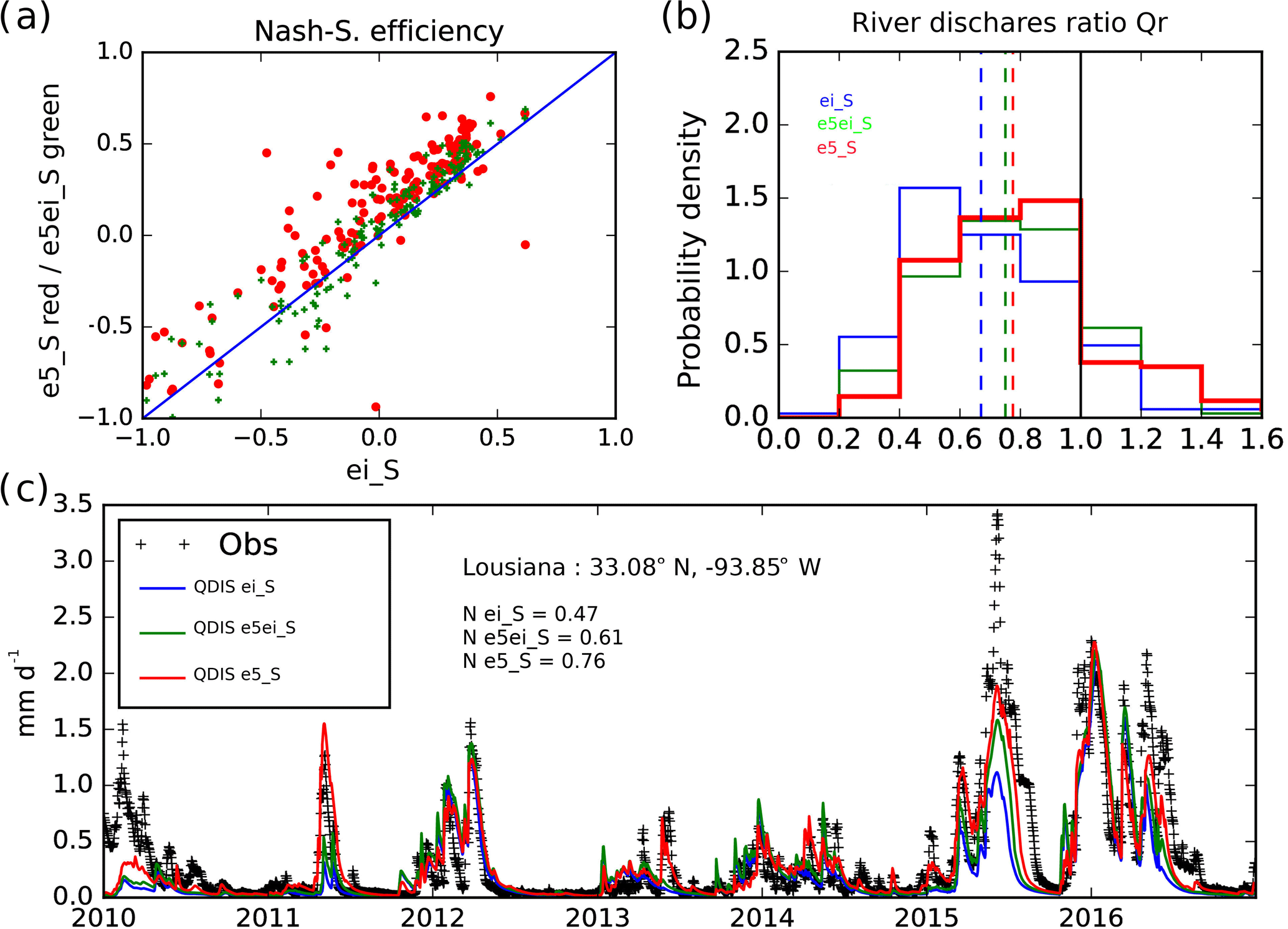
Figure 3 (a) Scatter plot of efficiency scores between in situ and simulated river discharges Q; efficiency scores for Q simulated with SURFEX forced either by ERA-5 but ERA-Interim precipitations (e5ei_S, green crosses) or ERA-5 (e5_S, red dots) as a function of efficiency scores for Q simulated using ERA-Interim (ei_S). (b) Histograms of river discharge ratio for ei_S (Qr_ei, in blue), e5ei_S (Qr_e5ei, in green) and e5_S (Qr_e5, in red). (c) Hydrograph for a river station in Louisiana (33.08^∘ N, 1.52^∘ W) representing scaled Q (using either observed or simulated drainage areas), in situ data (black crosses), simulated river discharges from ei_S (blue solid line), e5ei_S (green solid line) and e5_S (red solid line).

3.1 Evaluations using in situ measurements

This section presents the results of the comparison versus in situ observations of LSVs from model simulations using either ei_S, e5ei_S or e5_S starting with soil moisture. The statistical scores for 2010–2016 surface soil moisture from ei_S, e5ei_S and e5_S are presented in Table 2. Median R values on volumetric time series (anomaly time series) along with their 95 % confidence intervals are 0.66 ± 0.02 (0.53 ± 0.02), 0.69 ± 0.02 (0.54 ± 0.04) and 0.71 ± 0.02 (0.58 ± 0.03), while median ubRMSD are 0.052 ± 0.003, 0.052 ± 0.002 and 0.050 ± 0.003 for ei_S, e5ei_S and e5_S, respectively. These results underline the better capability of the ISBA LSM to represent surface soil moisture variability when forced by the ERA-5 reanalysis. Also, the latest configuration (e5_S) presents more stations with better R values on volumetric time series (anomaly time series) than both ei_S and e5ei, respectively 60 and 75 % (out of 110 and 107 stations, respectively). This is also reflected in Fig. 2, illustrating correlation values on volumetric time series (Fig. 2a) and anomaly time series (Fig. 2b) on maps. Star symbols represent stations for which ISBA LSM performs best when forced by ERA-Interim, circles when it is forced by ERA-5 with ERA-Interim precipitations and downward pointing triangles when it is forced by all ERA-5 atmospheric variables. Both maps in Fig. 2 are dominated by downward pointing triangles. Figure 2c and d show histograms of R differences on volumetric (anomaly) time series for soil moisture from e5_S (in red) e5ei_S (in green) with respect to ei_S, median values of the differences are also reported.

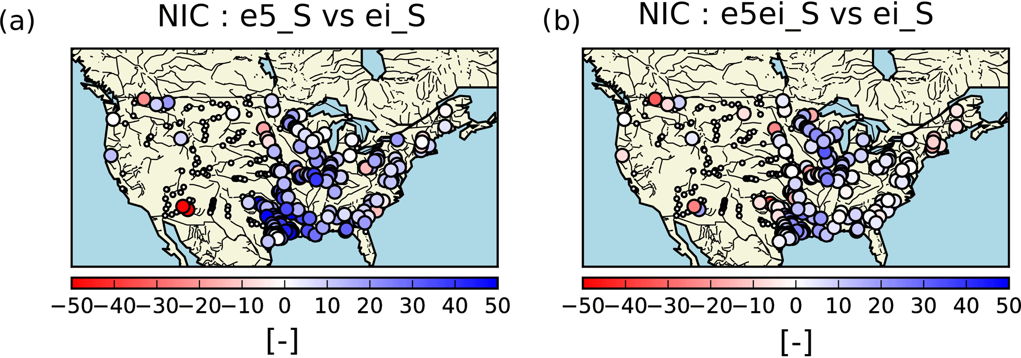
Figure 4 Normalized information contribution scores based on efficiency scores (NIC_NSE) (a) e5_S with respect to ei_S and (b) e5ei_S with respect to ei_S. Small dots represent stations for which the benchmark experiment (ei_S) present efficiency scores less than −1, large circles when it presents values more than −1. Positive values (blue large circles) suggest an improvement over ei_S, negative values (red large circles) a degradation. For sack of clarity, a factor of 100 has been applied to NIC.

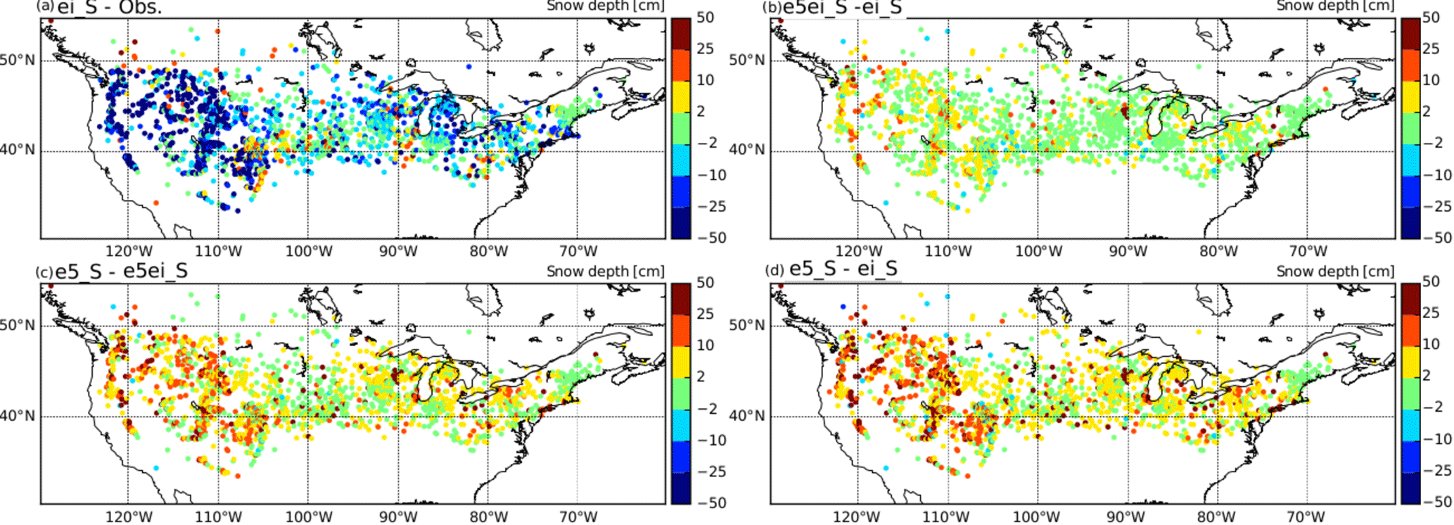
Figure 5 Mean snow depth bias for December–January–February in ei_S (a) and differences between e5ei_S and ei_S (b), e5_S and e5ei_S (c), and e5_S and ei_5 (d).

The 172 out of 344 gauging stations retained for the evaluation according to the criteria described in the methodology section present NSE scores in the [−1, 1] interval. Figure 3 presents the performance of each data set for this pool of stations. Figure 3a is a scatter plot of NSE scores between in situ and simulated river discharges Q; NSE scores for Q simulated with either ERA-5 but ERA-Interim precipitations (e5ei_S, green crosses) or ERA-5 (e5_S, red dots) as a function of NSE scores for Q simulated using ERA-Interim (ei_S). When considering e5_S, almost all the red dots are above the 1 : 1 diagonal, suggesting a general improvement from the use of e5_S. For a large part, e5ei_S green crosses are above this diagonal, suggesting that the improvement in e5_S does not only come from precipitation but also from other variables. Median NSE values are 0.06 ± 0.06, 0.12 ± 0.07 and 0.24 ± 0.05 for ei_S, e5ei_S and e5_S, respectively. Figure 3b shows an histogram of river discharge ratio for ei_S (Qr_ei in blue), e5ei_S (Qr_e5ei in green) and e5_S (Qr_e5 in red), median values are 0.67, 075 and 0.77, respectively. While all three experiments underestimate Q (a value of 1 being a perfect match), the use of e5ei_S and e5_S leads to better results. Finally, Fig. 3c illustrates hydrographs for a river station in Louisiana (33.08^∘ N, −93.85^∘ W) representing scaled Q (using either observed or simulated drainage areas), in situ data (black crosses), simulated river discharges from ei_S (blue solid line), e5ei_S (green solid line) and e5_S (red solid line). From this hydrograph, the added value of e5_S is clear, particularly for the 2011 and 2015 main events. NSE scores are 0.47, 0.61 and 0.76 for ei_S, e5ei_S and e5_S, respectively. Figure 4 illustrates the added value of using e5_S (panel a) or e5ei_S (panel b) with respect to ei_S. For 156 out of the pool of 172 stations, NIC_NSE values computed using e5_S with respect to ei_S are positive (large blue circles) showing a general improvement from the use of e5_S (representing 91 % of the stations) with a median NIC_NSE value of 14 % ± 0.05. When considering e5ei_S versus ei_S, they are still 118 (69 %) with a median NIC_NSE value of 4 % ± 0.02 suggesting that the improvement in e5_S does not only come from precipitation but also from other variables. It is also worth-noticing that stations where a score degradation is observed (large red circles) are located in areas known for irrigation, which is not represented in ISBA. All scores computed for seasons (December–January–February, March–April–May, June–July–August, September–October–November) suggest the same ranking (not shown).

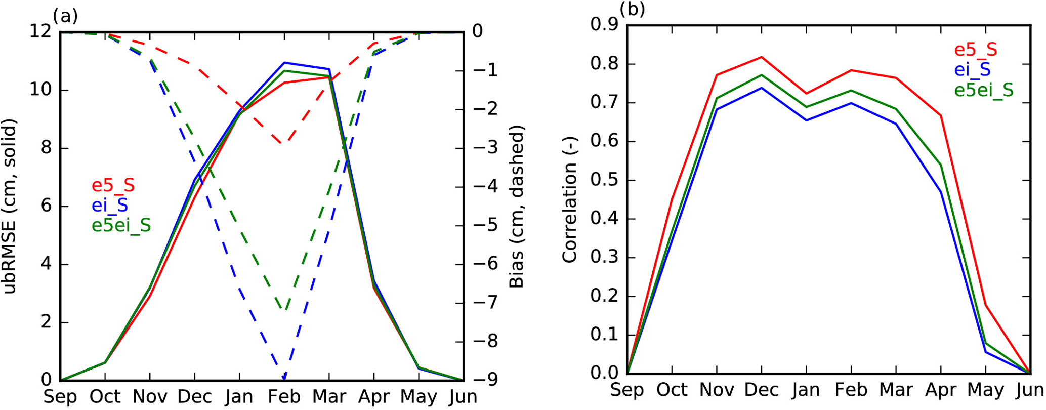
Figure 6 (a) Mean seasonal cycle of the bias (dashed lines) and ubRMSD (solid lines) averaged over all stations and (b) the mean seasonal cycle of the correlations for ei_S (in blue), e5ei_S (in green) and e5_S (in red).

Table 3 Comparison of snow depth with in situ measurements, median Bias, ubRMSD and R values are given for the three seasons affected by snow (SON, DJF, MAM) and for the whole period (All). SON, DJF and MAM stand for September–October–November, December–January–February and March–April–May, respectively.

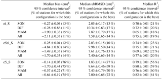
¹ only for stations presenting more than 80 % of (daily) data; 1901 out of 2056 stations. ² 95 % confidence interval of the median derived from a 10 000 samples bootstrapping.

The mean snow depth bias of ei_S (see Fig. 5) highlights a clear underestimation of winter snow depth accumulation mainly over the Rocky Mountains. This is likely a result of the underestimation of snowfall by ei_S associated with an overestimation of snow melt due to the coarse resolution of the ei_S reflected in a smooth topography. The replacement of all forcing variables by e5_S but keeping ei_S precipitation (e5ei_S, Fig. 5b) shows a slight increase in snow depth. This result justifies the above hypothesis that part of the snow underestimation is also due to temperature issues linked with a coarse model orography. Moving to the full e5_S forcing, there is a clear increase in snow depth when compared with both ei_S and e5ei_S forced simulations resulting from an increase in snowfall in e5_S. Figure 6 presents the mean seasonal cycle of bias and ubRMSD (Fig. 6a) and correlations (Fig. 6b) over the period 2010–2016. In addition to the added values of e5_S in terms of the mean snow depth already presented in Fig. 5, the temporal variability and random errors are also improved. Comparably with what was discussed for the mean bias, e5ei_S shows some benefits when compared with ei_S in terms of ubRMSD and correlation (median bias, ubRMSD and R values of e5ei_S over the whole period are −1.70 ± 0.33, 7.40 ± 0.65 and 0.77 ± 0.01 cm, respectively, for ei_S they are −2.11 ± 0.33, 7.58 ± 0.65 and 0.75 ± 0.01 cm, respectively), while e5_S has a clear improvement in ubRMSD and correlation (median bias, ubRMSD and R values of e5_ei over the whole period are −0.64 ± 0.19, 7.00 ± 0.65 and 0.82 ± 0.01 cm, respectively). The improvements on the snow depth simulations are consistent throughout the entire snow-cover season (see Fig. 6a and b) with a maximum improvement from January to March. These results highlight the cumulative effect of the forcing quality on the snow depth simulation. Finally Table 3 presents scores from the comparison of snow depth with in situ measurements; median bias, ubRMSD and R values are given for the three seasons affected by snow (September–October–November, December–January–February and March–April–May) and for the whole period. e5_S always presents better scores when compared to ei_S and it is always the configuration presenting the highest percentage of stations with the best scores. Looking at the 95 % confidence interval, for the correlation and bias, it is clear that the changes are significant.

Table 4 Comparison of sensible (H) and latent (LE) heat flux with in situ observations for ei_S, e5ei_S and e5_S. Median correlations (R) and median RMSD are given for the FLUXNET stations. Scores are given for significant correlations with p values < 0.05.

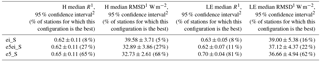
¹ only for stations presenting significant R values (p value < 0.05): 37 stations; ² 95 % confidence interval of the median derived from a 10 000 samples bootstrapping

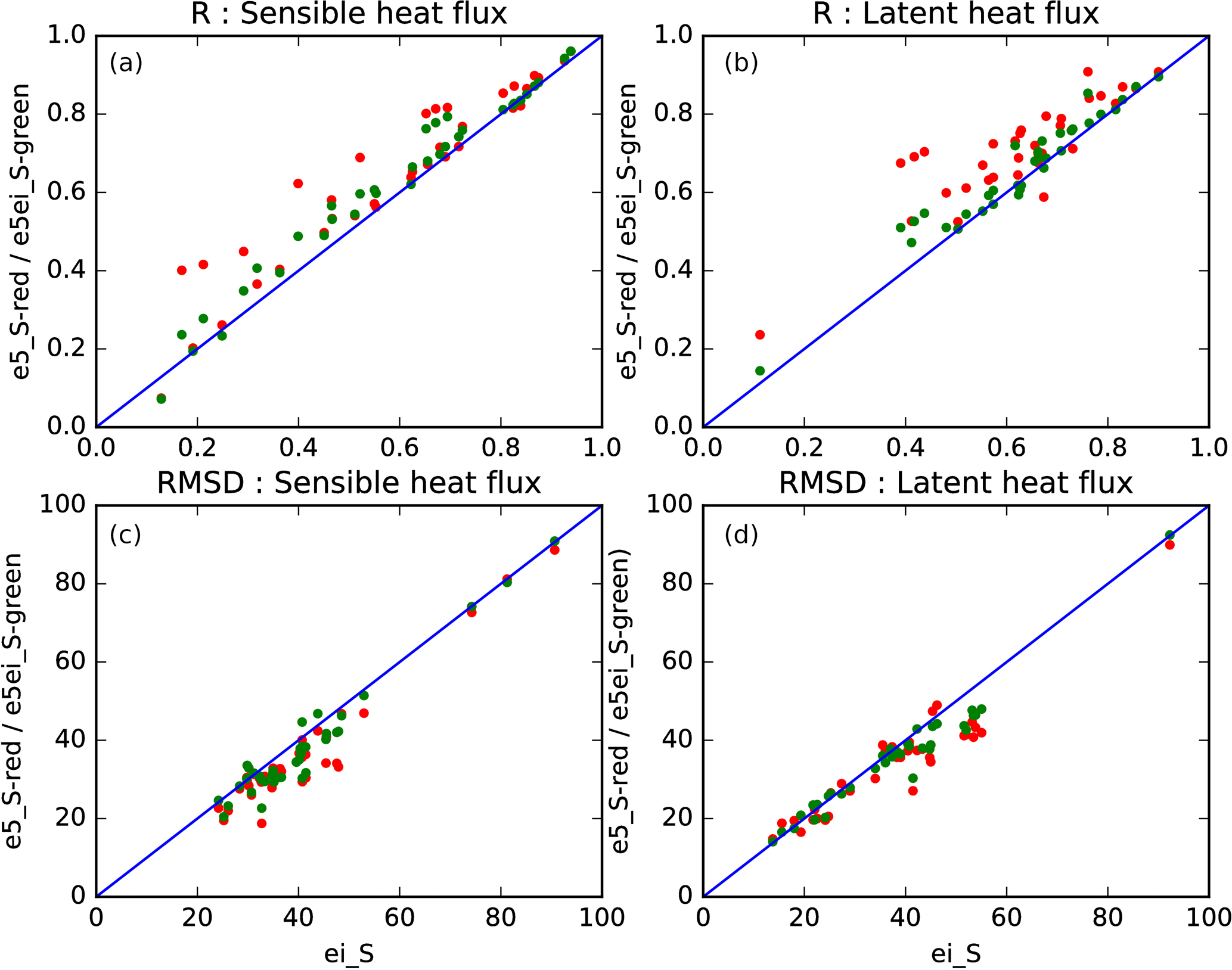
Figure 7 Scatter plots illustrating evaluation of ei_S, e5ei_S and e5_S against in situ measurements of sensible (a for correlation, c for RMSD) and latent (b for correlation, d for RMSD) heat flux. Scores for either e5ei_S (green dots) or e5_S (in red) are presented as a function of those for ei_S.

Results from the comparisons between ei_S, e5ei_S, e5_S and in situ sensible and latent flux measurements are presented in Table 4 and illustrated by Fig. 7. The 37 stations present significant correlation values (at p value < 0.05). For sensible heat flux, median correlation and RMSD values are 0.62 ± 0.11, 0.62 ± 0.11 and 0.65 ± 0.11 and 39.58 ± 3.71, 32.89 ± 3.86 and 32.73 ± 2.61 W m⁻² for ei_S, e5ei_S and e5_S, respectively. For latent heat flux, they are 0.63 ± 0.05, 0.62 ± 0.07 and 0.70 ± 0.04 and 39.00 ± 5.38, 37.12 ± 4.37 and 36.66 ± 4.94 W m⁻², respectively. As for surface soil moisture, river discharge and snow depth, e5_S presents better results than e5ei_S and ei_S. At the station level, Fig. 7 illustrates scatter plots of correlations and RMSD for sensible and latent heat flux from ei_S, e5ei_S, e5_S against in situ measurements of sensible (Fig. 7a for correlation, Fig. 7c for RMSD) and latent (Fig. 7b for correlation, Fig. 7d for RMSD) heat flux. Scores for either e5ei_S (green dots) or e5_S (in red) are presented as a function of those for ei_S. When looking at the correlations, almost all of e5_S and e5ei_S symbols (in red and green, respectively, in Fig. 7a, c) are above the 1 : 1 diagonal indicating that e5_S and e5ei_S better represent sensible and latent heat flux than ei_S. The same tendency is observed for RMSD with most of the symbols below the 1 : 1 diagonal. If RMSD values are comparable for e5_S and e5ei_S, R values are clearly higher for e5_S.

Figure 8 Seasonal correlations for (a) volumetric time series and (b) anomaly time series between surface soil moisture (SSM) estimates from the ESA CCI project (ESA CCI SSM v4) and soil moisture from the second layer of soil of the ISBA LSM forced by ERA-Interim (ei_S, in blue), ERA-5 but with precipitation from ERA-Interim (e5ei_S, in green) and ERA-5 (e5_S, in red) over the period 2010–2016. Maps of correlation differences between soil moisture from e5_S and ei_S for volumetric time series (c) and anomaly time series (d) are shown, areas in red represent an improvement from the use of ERA-5. Grey areas represent areas that were flagged out for elevation greater than 1500 m above sea level.

3.2 Evaluations using satellite-derived estimates

Figure 8 illustrates the comparison between ESA CCI SSM v4 and soil moisture from the ISBA second layer of soil over 2010–2016. Figure 8a shows seasonal correlations on volumetric time series and Fig. 8b on anomaly time series. Scores for ISBA LSM forced by ERA-Interim (ei_S) are in blue, ERA-5 but with precipitation from ERA-Interim (e5ei_S) in green and ERA-5 (e5_S) in red. From Fig. 8a, one can appreciate the added value of using ERA-5 atmospheric forcing particularly from April to September. It is also interesting to notice that when using all ERA-5 atmospheric fields except for the precipitation, a similar added value is noticeable suggesting that all improvements from ERA-5 do not only come from precipitation. However, when evaluating the short-term variability of soil moisture (i.e. removing the seasonal effect), it is really ERA-5 that provides the best results. Correlation on volumetric (anomaly) time series for all grid points put together over 2010–2016 are 0.668 (0.464), 0.682 (0.468) and 0.689 (0.490) for ei_S, e5ei_S and e5_S, respectively. Additionally to the global seasonal scores, Fig. 8c and d present maps of correlation differences between soil moisture from e5_S and ei_S on volumetric time series and anomaly time series, respectively. Grey areas represent areas that were flagged out for elevation greater than 1500 m above sea level. As visible on Fig. 8c and d, the use of ERA-5 mainly leads to improvements all over the considered domain. Focusing on correlation differences, (R_e5−R_ei) on volumetric (or anomaly) time series, 68 % (77 %) of the values are positive – indicating an improvement from e5_S – with median values of 4.5 % (4.11 %) and include values up to 40 % (45 %). It shows the added value of using ERA-5 to force ISBA LSM compared to ERA-Interim.

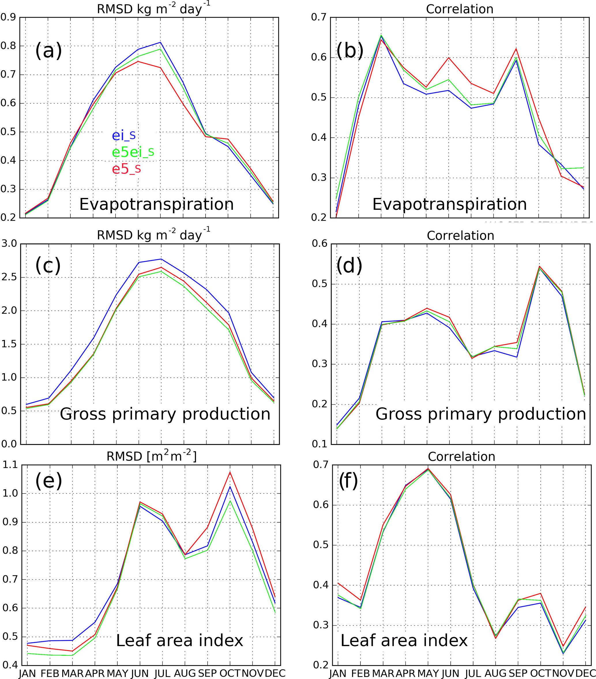
Figure 9 Seasonal scores between ISBA LSM within SURFEX forced by either ERA-Interim (ei_S, in blue), ERA-5 but ERA-Interim precipitation (e5ei_S, in green) or ERA-5 (e5_S, in red) and (a, b) evapotranspiration estimates from the GLEAM project over the period 2010–2016, (c, d) upscaled GPP from the FLUXCOM project over 2010–2013 and (e, f) LAI estimates from the CGLS project over 2010–2016. The left column (a, c, e) are for RMSD and the right column (b, d, e) are for correlations.

Figure 9 illustrates seasonal scores between ISBA LSM forced by either ERA-Interim (ei_S in blue), ERA-5 but ERA-Interim precipitation (e5ei_S in green) or ERA-5 (e5_S in red) for the following variables: (Fig. 9a, b) evapotranspiration estimates from the GLEAM project over 2010–2016, (Fig. 9c, d) upscaled GPP from the FLUXCOM project over 2010–2013 and (Fig. 9e, f) LAI estimates from the CGLS project over 2010–2016. The left column (Fig. 9a, c and e) are for RMSDs and the right column (Fig. 9b, d and e) for correlations. For evapotranspiration, and to a lesser extend GPP, one can notice a decrease in RMSD when using ERA-5 atmospheric reanalysis compared to ERA-Interim atmospheric reanalysis; however, it fails at improving LAI. Considering evapotranspiration, correlation (RMSD) values for all grid points put together over 2010–2016 are 0.786 (0.927 kg m⁻² d⁻¹), 0.778 (0.917 kg m⁻² d⁻¹) and 0.795 (0.889 kg m⁻² d⁻¹) for ei_S, e5ei_S and e5_S, respectively. They are 0.726 (2.429 kg m⁻² d⁻¹), 0.733 (2.167 kg m⁻² d⁻¹) and 0.734 (2.227 kg m⁻² d⁻¹) for GPP and 0.715 (1.050 m² m⁻²), 0.710 (1.026 m² m⁻²) and 0.697 (1.079 m² m⁻²) for LAI, respectively.

Improvements (in red) and degradations (in blue) from the use of ERA-5 in the ISBA LSM with respect to ERA-Interim for evapotranspiration, GPP and LAI are illustrated by Fig. 10 (respectively from top to bottom). Figure 10a, c and e show RMSD differences while Fig. 10b, d and f show R differences. Both differences in RMSD and R values suggest an improvement from the use of ERA-5 as the two figures are mainly dominated by red colours, RMSD and R represent 56 and 53 % of the domain, respectively for evapotranspiration (Fig. 10a, b), 60 and 69 % for GPP (Fig. 10c, d), but only 47 and 44 % for LAI (Fig. 10e, f).

4 Discussion and conclusions

This study assesses the ability of the recently released ERA-5 atmospheric reanalysis to force the ISBA land surface model (LSM) with respect to ERA-Interim reanalysis over North America for 2010–2016. The results presented above using the three atmospheric reanalysis data sets (ERA-Interim, ei_S; ERA-5 but with precipitation from ERA-Interim, e5ei_S; and ERA-5, e5_S, with all meteorological variables) to force the ISBA LSM provide two important insights: (i) firstly the use of ERA-5 leads to significant improvements in the representation of the land surface variables (LSVs) linked to the terrestrial water cycle assessed in this study (surface soil moisture, river discharges, snow depth and turbulent fluxes) but failed impacting LSVs linked to the vegetation cycle (carbon uptake and LAI). Even when they are small, improvements are systematic when using ERA-5. (ii) Secondly, if most of the improvements seem to come from a better representation of the precipitation in ERA-5, the e5ei_S experiment also presents improvements with respect to the ei_S experiment and suggests that the other meteorological forcing from ERA-5 are better represented too. However, it is acknowledged that the use of 3-hourly ERA-Interim liquid and solid precipitations rescaled at an hourly time step in ERA-5 might have sometimes led to inconsistent configurations (e.g. precipitations while having a very strong net radiation).

ERA-5 has a great potential to further improve the representation of LSVs if used to force offline LDAS. In recent years, several LDAS have emerged at different spatial scales, (i) regional like the Coupled Land Vegetation LDAS (CLVLDAS; Sawada and Koike, 2014, Sawada et al., 2015) and the Famine Early Warning Systems Network (FEWSNET) LDAS (FLDAS; McNally et al., 2017), (ii) continental like the North American LDAS (NLDAS; Mitchell et al., 2004; Xia et al., 2012) and the National Climate Assessment LDAS (NCA-LDAS; Kumar et al., 2018), and (iii) global like the Global Land Data assimilation (GLDAS; Rodell et al., 2004) and more recently LDAS-Monde (Albergel et al., 2017, 2018). LDAS-Monde is a global capacity system able to sequentially assimilate satellite-derived estimates of surface soil moisture and LAI. Albergel et al. (2017) found that the main improvements of their analysis (i.e. with assimilation) when compared to an open-loop experiment (simple model run) were linked to vegetation variables and the assimilation of vegetation estimates. They have also proposed further advances on a better use of satellite-based microwave data in the assimilation system. Having LDAS-Monde analysis forced by ERA-5 atmospheric forcing should both combine the strengths of an improved atmospheric reanalysis on the terrestrial water cycle and of the assimilation of satellite-derived products on the vegetation cycle. Effort will now be concentrated on the use of ERA-5 and strengthening LDAS-Monde through the direct assimilation of satellite-based soil moisture and vegetation properties from microwave remote sensing. It will enable fostering links with potential applications like climate reanalysis of the LSVs as well as going from a monitoring system of the LSVs and extreme events (like agricultural drought) to a forecasting system. Preliminary results suggest that a LSV forecast initialized by an analysis is more robust than one initialized by a simple model run (Albergel et al., 2018). Preliminary tests over Europe also indicate similar benefits from the use of ERA-5 (not shown). When the whole ERA-5 period will be available (1979–present), in addition to the availability of the ERA-5 10-member ensemble of data assimilation (at lower spatial and temporal resolutions though), it will be possible to develop a global long-term ensemble of LSV reanalysis forced by high quality atmospheric data. It will make it possible providing uncertainties in the representation of the atmospheric forcing, while LSVs may require special considerations and perturbation methods. Capturing those uncertainties coming from the simplifications and assumptions in the LSM is of paramount interest for many applications from monitoring to forecasting.