Hydrostratigraphic modeling using multiple-point statistics and airborne transient electromagnetic methods

Creating increasingly realistic groundwater models involves the inclusion of additional geological and geophysical data in the hydrostratigraphic modeling procedure. Using multiple-point statistics (MPS) for stochastic hydrostratigraphic modeling provides a degree of flexibility that allows the incorporation of elaborate datasets and provides a framework for stochastic hydrostratigraphic modeling. This paper focuses on comparing three MPS methods: snesim, DS and iqsim. The MPS methods are tested and compared on a real-world hydrogeophysical survey from Kasted in Denmark, which covers an area of 45 km². A controlled test environment, similar to a synthetic test case, is constructed from the Kasted survey and is used to compare the modeling results of the three aforementioned MPS methods. The comparison of the stochastic hydrostratigraphic MPS models is carried out in an elaborate scheme of visual inspection, mathematical similarity and consistency with boreholes. Using the Kasted survey data, an example for modeling new survey areas is presented. A cognitive hydrostratigraphic model of one area is used as a training image (TI) to create a suite of stochastic hydrostratigraphic models in a new survey area. The advantage of stochastic modeling is that detailed multiple point information from one area can be easily transferred to another area considering uncertainty.

The presented MPS methods each have their own set of advantages and disadvantages. The DS method had average computation times of 6–7 h, which is large, compared to iqsim with average computation times of 10–12 min. However, iqsim generally did not properly constrain the near-surface part of the spatially dense soft data variable. The computation time of 2–3 h for snesim was in between DS and iqsim. The snesim implementation used here is part of the Stanford Geostatistical Modeling Software, or SGeMS. The snesim setup was not trivial, with numerous parameter settings, usage of multiple grids and a search-tree database. However, once the parameters had been set it yielded comparable results to the other methods. Both iqsim and DS are easy to script and run in parallel on a server, which is not the case for the snesim implementation in SGeMS.

1 Introduction

Recent advances in groundwater modeling have shown the importance of accurate hydrogeologic models for management of increasingly sparse groundwater resources. Groundwater modeling predictions are sensitive to geologic heterogeneity (e.g., Freeze, 1975; Gelhar, 1984; Fogg et al., 1998; LaBolle and Fogg, 2001; Zheng and Gorelick, 2003; Feyen and Caers, 2006; Fleckenstein et al., 2006; Zhao and Illman, 2017). However, geological units include complexities not directly related to hydrofacies (Klingbeil et al., 1999). Instead, the concept of hydrostratigraphic units is used throughout this study, which effectively combines geological units and reduces the total number of units resulting in a closer relation to the hydrologic units. Improving the realism and quantification of uncertainty around hydrostratigraphic models is therefore an important step towards accurate groundwater modeling predictions. Hydrostratigraphic models are created using several approaches. A common approach is a manual co-interpretation of available geophysical, geological and/or hydrologic data. The geoscientist cognitively uses his/her refined knowledge of geological processes combined with the provided datasets to create a detailed cognitive geological model (e.g., Jørgensen et al., 2013; Royse, 2010). The cognitive geological model is then simplified to a hydrostratigraphic model. Even though the hydrostratigraphic model encapsulates the complexities related to geologic architecture, it does not reflect the hydrostratigraphic uncertainty. It is a so-called deterministic model, i.e., one version of the hydrostratigraphic subsurface. An alternative to cognitive modeling is stochastic modeling using geostatistical methods. The field of geostatistical modeling focuses on creating models depicting subsurface hydrogeology and/or reservoir properties. Geostatistics is currently applied in a number of geoscience fields, such as petrology (e.g., Okabe and Blunt, 2005), petroleum reservoir modeling (e.g., Journel and Zhang, 2006; Strebelle et al., 2002), hydrogeology (e.g., Huysmans and Dassargues, 2009) and hydrology (e.g., Michaelides and Chappell, 2009). Overall geostatistical methods provide a framework in which multiple equiprobable hydrostratigraphic models can be created in a semiautomated fashion. The individual stochastic models do not reflect the modeling uncertainty, but the model ensemble does. The multiple hydrostratigraphic models can be used as a set of input parameters for the groundwater model. By running the groundwater model several times with different hydrostratigraphic models, multiple predictions can be made, yielding an estimate of the prediction uncertainty. The ability to understand how the hydrostratigraphic uncertainty is related to the prediction uncertainty will help in understanding where to improve the hydrostratigraphic models in order to reduce the prediction uncertainty. This study will however not focus on groundwater modeling predictions, but on the presentation of a stochastic modeling framework for reconstructing subsurface hydrostratigraphic architecture.

Today state-of-the-art geostatistical tools are readily available to geoscientists. Traditional two-point statistics, or variogram-based methods, e.g., sisim (Journel, 1983) and sgsim (Deutsch and Journel, 1998), have been widely used in both research and in practice (e.g., Seifert and Jensen, 1999; Caers, 2000; Juang et al., 2004; Delbari et al., 2009). However, variogram-based techniques depend on two-point statistics for simulation of complex geological features. Depending on the complexity of the geological setting, such two-point statistical methods cannot recreate complex curvilinear geological features of the subsurface which are common in fluvial and glaciofluvial environments (e.g., Arpat and Caers, 2005; Hu and Chugunova, 2008; Journel and Zhang, 2006; Journel, 1993; Liu, 2006; Sánchez-Vila et al., 1996; Strebelle and Journel, 2001). An additional geostatistical modeling tool which should be mentioned is T-PROGS (Carle, 1999). T-PROGS is based on transition probabilities between categories and generates geostatistical realizations based on such constraints. In comparison with the indicator method, sisim, it allows for better integration of these transition probabilities and, hence, the spatial cross-correlations of soil/rock-type architecture into the groundwater models. However, T-PROGS also has difficulties in reconstructing curvilinear geological features. Kessler et al. (2013) made a detailed comparison between T-PROGS realizations and real-world cross sections in a gravel pit in Denmark. The result reveals a suboptimal pattern reproduction, in comparison to other simulation tools such as multiple-point statistics (MPS) (Mariethoz and Caers, 2014b). MPS is a recent alternative to classic two-point statistics. Here, additional multiple-point (MP) information from a training image (TI) is used to condition the simulations. The usage of MP information allows for reconstruction of more complex geological features, such as curvilinear features (Strebelle, 2002). A TI is any 2-D or 3-D image containing geometrical information relevant to the hydrostratigraphic model. The crux of the MPS approach is finding a relevant TI. Some examples of 2-D and 3-D TIs are categorical images of outcrops (2-D), categorical drawings of a geological system created by a geoscientist (2-D), and cognitive geological or hydrostratigraphic voxel models (3-D) (e.g., Høyer et al., 2015a). Today, MPS techniques are widely used in geoscientific research and studies, a few examples are Maharaja (2005), Meerschman et al. (2013) and Hermans et al. (2014). The MPS framework allows for conditioning of geological architecture/patterns, a stochastic framework and spatially constraining to both soft data and hard data (Arpat and Caers, 2005; Guardiano and Srivastava, 1993; Journel, 1993; Strebelle and Journel, 2001).

Within the geostatistics framework the creation of hydrostratigraphic models requires the inclusion of data from multiple sources, often geophysical models (soft data), borehole data (hard data) and a TI. The different data sources each provide relevant information. Geophysical models provide information regarding the large-scale hydrostratigraphic architecture. Boreholes, on the other hand, provide detailed yet usually sparse information regarding hydrostratigraphic units. Each data source is a piece of the puzzle; combining the individual pieces improves the resulting hydrostratigraphic models. The inclusion of several types of data is, however, not trivial since information regarding their mutual relationships, e.g., the hydrostratigraphic–petrophysical relationship, is required. An important source of information which helps to combine the different sources of data is geologic knowledge. Geologic knowledge can be defined as information regarding geologic processes, geomorphologic patterns and structural geology. Incorporating geological knowledge into hydrostratigraphic models is often difficult and done ad hoc. Geologic information, as described above, complements the soft data and helps to create more realistic hydrostratigraphic models. However, within the MPS framework this type of information can be implemented via the TI.

This study focuses on comparing and testing three MPS methods on a real-world dataset from a groundwater survey in Kasted, Denmark. An important part of the dataset is the airborne geophysical survey, providing a set of resistivity models containing information regarding the large-scale hydrostratigraphic architecture of the area. The MPS tools are used to reconstruct an intricate system of interconnected buried valleys. The end result is an ensemble of hydrostratigraphic models. A 3-D hydrostratigraphic voxel model of the area is used as a TI, containing detailed MP information regarding the hydrostratigraphic features of the survey area. Information regarding the geological architecture and the relationship between hydrostratigraphy and petrophysical properties are contained in the TI. The hydrostratigraphic–petrophysical relationship is explicitly known since the hydrostratigraphic model spatially overlaps with the geophysical and borehole lithology logs. Spatially constraining the simulation to the soft data, consisting of the resistivity models, ensures that simulated geological patterns are placed concurrently to the real world. However, such geophysical soft data have several types of related uncertainty, e.g., spatial uncertainty related to incomplete datasets, resolution capabilities and signal-to-noise ratio decrease with depth. Incomplete geophysical datasets are a common problem and are typically reconstructed using geostatistics – often in a deterministic fashion. A common approach is to use variogram-based geostatistics, such as kriging interpolation, to reconstruct the incomplete resistivity grid (Isaaks and Srivastava, 1989). We have used the stochastic direct sampling (DS) grid reconstruction routine proposed by Mariethoz and Renard (2010). Here, the grid reconstruction uncertainty is reflected by multiple resistivity grids, yielding variable patterns in the multiple reconstructed grids. The reconstructed grids are then used in conjunction with the hydrostratigraphic TI to create a set of stochastic hydrostratigraphic realizations of the hydrostratigraphy of the modeled area.

In relation to the Danish groundwater mapping campaign (Thomsen et al., 2004), detailed geophysical datasets (Møller et al., 2009) and hydrostratigraphic models exist. A selection of the 3-D geologic and hydrostratigraphic voxel models is reported in the literature (e.g., Høyer et al., 2015a, b; and Jørgensen et al,. 2015). Additionally, the study by Høyer et al. (2017) presents a framework for making large-scale MPS models based on geological 3-D voxel models, as well as seismic and borehole data. In this study, we will show how MPS methods can be utilized to model a new survey area. An existing cognitive model from one area is used as a TI for simulating another survey area with similar geological characteristics.

To our knowledge, no vigorous studies comparing multiple MPS methods have been carried out on real-world hydrogeophysical datasets. By applying several measures to assess and compare the modeling results, the selected MPS tools are tried, tested and compared on real-world data. The MPS methods are tested in a pseudo-synthetic environment, where an actual 3-D hydrostratigraphic model of the Kasted survey area is used as a TI. This guarantees a controlled modeling environment in which the TI contains highly relevant hydrostratigraphic architecture. The main contributions of this study are (1) a practical real-world example of stochastic reconstruction of incomplete geophysical datasets; (2) comparison of three MPS methods for integrating geophysical data – snesim (Liu, 2006; Strébelle and Journel, 2000), direct sampling (DS) (Mariethoz et al., 2010) and image quilting (iqsim) (Hoffimann et al., 2017; Mahmud et al., 2014); (3) validation of the comparison results by (a) visual inspection, (b) a mathematical comparison method called the analysis of distance (ANODI) (Tan et al., 2014) and (c) comparison of the simulation results against the borehole lithology logs; and (4) to show the strengths and weaknesses of a stochastic hydrostratigraphic modeling framework, and (5) an example using the direct sampling method and showing how to use the cognitive hydrostratigraphic interpretation of one area to directly generate hydrostratigraphic models of new areas, using only the soft data from the new area.

2 Study area and data

The Kasted survey area is located in Denmark, in the eastern part of Jutland, close to the city of Aarhus (Fig. 1a). The 45 km² area has been surveyed in detail and contains 453 boreholes as well as a SkyTEM survey of 333 line km. A detailed geologic model of the area has been created by Høyer et al. (2015a). The dataset was collected and compiled in relation to the HyGEM project. The local geology consists of an intricate system of interconnected Quaternary buried valleys, infilled with till and meltwater deposits. The buried valleys are incised into thick hemipelagic Paleogene clay, which dominates the area (Høyer et al., 2015a). Many such pre-glaciated areas are dominated by buried valleys, which have proven important subsurface features in regard to groundwater flow (Jørgensen and Sandersen, 2006; Seifert et al., 2008). These noteworthy geological features have received a lot of attention in research through the years (e.g., Destombes et al., 1975; Jørgensen and Sandersen, 2009; Kehew et al., 2012; Ritzi et al., 1994).

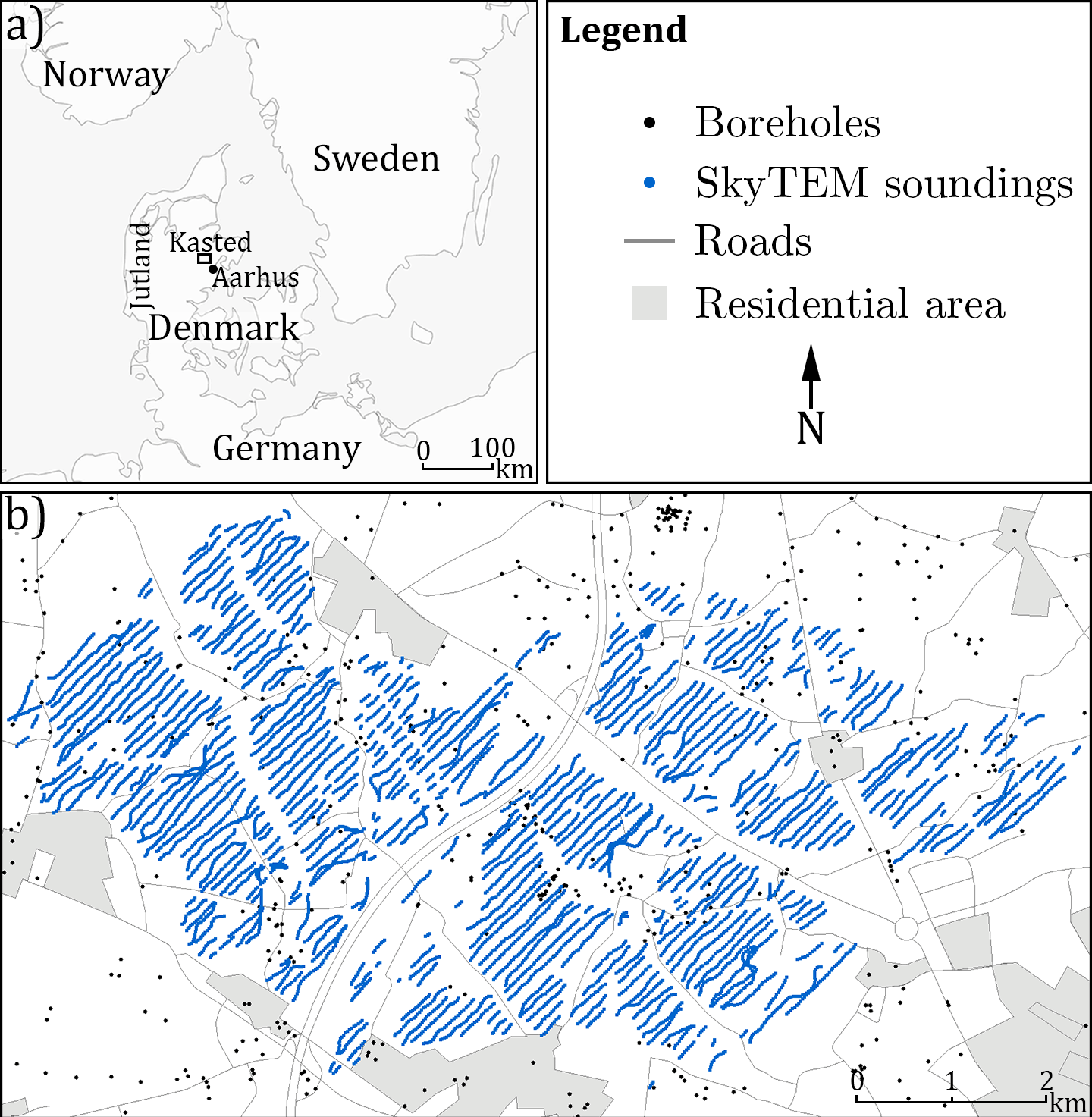
Figure 1 An overview map of the Kasted survey area. (a) shows the geographic location of the survey area, which is marked as a black box; and (b) shows a close-up view of the Kasted survey area with the related datasets and infrastructure overlay.

The dataset used in this study consists of a dense airborne geophysical SkyTEM survey, near-surface boreholes from the Danish borehole database, and a cognitive geologic model created by an experienced geoscientist. In the following we will summarize the key features of these datasets.

The SkyTEM system (Sørensen and Auken, 2004) is a helicopter transient electromagnetic system allowing for rapid collection of large geophysical datasets, with high spatial density. The Kasted SkyTEM survey contains 333 line km with a line spacing of roughly 100 m (Fig. 1b). The SkyTEM data are inverted and modeled according to the scheme described by Viezzoli et al. (2008), with the end result being a collection of spatially constrained inversion models. In Denmark it is standard protocol to calibrate the SkyTEM system at an official calibration site, as described by Foged et al. (2013), ensuring data of high-quality and reproducible results. Therefore, the resistivity values from a calibrated SkyTEM survey are comparable to other calibrated SkyTEM surveys. The SkyTEM system is sensitive towards large-scale conductive trends in the subsurface, especially when a significant contrast between a conductive and a resistive feature exists. In the eastern part of Jutland it is common that the lower confining boundaries of the buried valleys are well resolved since these buried valleys are often quite resistive and are eroded into conductive hemipelagic Paleogene clays.

The Danish borehole database, JUPITER (Hansen and Pjetursson, 2011), contains about 280 000 shallow boreholes which have been drilled for a variety of purposes, mainly in relation to drinking water and raw materials exploration, but also in relation to research and geotechnical studies. The JUPITER database contains information on location, drilling method, lithology, geologic age, filter position and water chemistry.

The cognitive geologic model was created using all available data, including the 333 line km of SkyTEM data, information from 435 boreholes and prior geological knowledge of the area. The model was created using the cognitive modeling scheme, which is introduced by Jørgensen et al. (2013). The geological model is described in great detail by Høyer et al. (2015a). The geologic model is detailed and contains a set of 21 interconnected buried valleys. The final 3-D voxel model contains 42 unique geological units, which are simplified into three overall hydrostratigraphic units in this study. The three hydrostratigraphic units are chosen for the purpose of covering the overall hydrogeological features of the groundwater modeling area. The cognitive hydrostratigraphic model will act as the TI as well as a baseline for assessing the performance of the three MPS methods, and the stochastic modeling results will be compared against the cognitive model.

3 Methods

MPS provides a degree of flexibility, which assists the modeler in creating geologically realistic hydrostratigraphic models. The idea is to create a suite of hydrostratigraphic models, which span a realistic subset of possible model architectures, as opposed to a deterministic model, which spans a single possible model architecture. The term realistic refers to models, which comply with the underlying datasets mentioned above, i.e., borehole lithological logs, geophysical resistivity models and the cognitive geological model. The underlying datasets have associated uncertainties describing ranges of possible models. The suite of equiprobable hydrostratigraphic models can be used as input to a groundwater model, making it straightforward to test the sensitivity of specific groundwater model predictions.

3.1 MPS methodologies

MPS methods use a training image to condition a model simulation to a prior geological conceptualization. As opposed to two-point statistics, the joint variabilities of multiple points are assessed at the same time during simulation. The MP joint variabilities cannot be inferred from sparse data and are therefore taken from a relevant exhaustive TI. The justification that a given TI can be used to infer the joint variability of MPs heavily lies on the choice of a relevant TI. A TI should always contain geologically realistic and relevant information (Journel and Zhang, 2006). Finding and/or creating a realistic TI is thus important to the MPS methodology. A TI is essentially any categorical or continuous image. which contains the geological conceptualization of the target variable (Mariethoz and Caers, 2014a). It is not a subsurface model itself, but a quantitative conceptual depiction of it. The user chooses the TI based on his/her prior understanding of the local hydrogeological system. The TI does not need to carry any locally accurate information; i.e., it does not need to contain the actual geographical positions of the hydrostratigraphic architecture, just the general patterns. It needs to reflect a prior geological or structural concept (Strebelle and Journel, 2001).

The MPS methods chosen in this study have been selected to reflect recent advances in MPS methods. The MPS methods in this study include the single normal equation simulation (snesim) (Strébelle and Journel, 2000) implemented in the Stanford Geostatistical Modeling Software (SGeMS), direct sampling simulation (DS) (Mariethoz et al., 2010) implemented in the DeeSse software package (Straubhaar, 2011) and image quilting simulation (iqsim) (Hoffimann et al., 2017) implemented in ImageQuilting.jl.

3.1.1 Single normal equation simulation – snesim

The snesim method is a traditional MPS method. It fits into the so-called “probability framework” where geophysical models (not data) are considered soft information, and as such needs to be converted into probabilities. Suppose we have a categorical random variable S which has K possible states ($s_k,k=\mathrm{1},\mathrm{\dots },K)$; i.e., there are K hydrostratigraphic units. For each cell in the target sampling grid a probability prob{s_k} is defined for each of the K states, so that for a given grid cell, denoted cell_i,

$$\begin{array}{}\text{(1)}& \mathrm{prob}\left\{{\mathrm{cell}}_i\right\}={\sum }_{k=\mathrm{1}}^K\mathrm{prob}\left\{s_k\right\}=\mathrm{1},\end{array}$$

where $i\in \left\{\mathrm{1},\mathrm{\dots },N\right\}$, and the sampling grid has a total of N cells. The crux is then to translate the geophysical data into the probabilities described in Eq. (1). The collection of all probabilities for the entire sampling grid is also referred to as a probability map (2-D) or probability grid (3-D). The translation of the soft data is usually carried out based on a prior understanding of the petrophysical–hydrostratigraphic relationship and will be discussed further later in the paper. For a detailed description of the more general petrophysical–lithological relationship, the reader is referred to Barfod et al. (2016) and Beamish (2013). The probability grids are used to constrain the simulation using the so-called tau model (Journel, 2002). The probability grid approach is intuitive and allows the modeler to incorporate any desired datasets or variables into the probability map. Examples of soft data are any type of geophysical soft data and/or prior information, which can be translated into probabilities.

In snesim, the TI is stored in a dynamic data structure called a search tree. The search tree is a database and can be seen as a condensed summary of the full TI. It contains the spatial information to which the simulation is conditioned; for more detail see Strebelle (2002). To avoid repetitive scanning of the TI, which is computationally expensive, the TI is stored in a search-tree database ahead of the simulation (Roberts, 1998). This is done once. TI patterns can then be retrieved from the database without scanning the entire TI. Depending on the amount of detail stored in the search tree this can be quite CPU intensive, since the entire search tree is stored in memory, and therefore there is an upper limit to the size of the search-tree pattern database. However, advances in computers have increased the upper limit for available CPU.

Another caveat of snesim is the usage of multiple grids (Tran, 1994). Due to limitations in relation to the search neighborhood, the simulation of structures on all scales requires the usage of multiple grids. The simulation is carried out on a series of multiple simulation grids with varying density, ensuring pattern reproduction at all scales. The search-tree formulation and multiple grid approach add to the overall complexity of parameterization in snesim, but at the same time ensure stable and reliable MPS modeling results. The increased number of user-defined parameters makes it less intuitive, since it is relatively difficult to determine the optimal parameter values for a given dataset.

3.1.2 Direct sampling simulation – DS

The direct sampling simulation (DS) method consists, for the simulation of each cell, in randomly scanning the TI until a pattern similar to the pattern centered at the simulated cell is found and then in copying the value in the center of the pattern from the TI to the simulation grid. Consequently, contrary to snesim, no probability is explicitly computed to draw a value at a simulation grid cell. In this paper, we use the DeeSse implementation of DS, presented by Straubhaar (2011). This bypasses the necessity of saving spatial patterns in a search-tree database; instead, spatial patterns are conditioned by directly scanning the TI.

One issue which needs to be solved is how to constrain a soft data variable. In DS, this is accomplished by introducing an auxiliary variable. The auxiliary variable is roughly a translation of the TI into a soft data variable. Suppose a forward operator, denoted by G, represents the physical model, which translates the subsurface hydrostratigraphic units into the continuous soft data variable, as when scanning the near surface with a geophysical instrument and subsequently processing and interpreting the data into the actual petrophysical parameters. Then we can define an approximate forward operator G^∗ (Mariethoz and Caers, 2014b). The G^∗ operator is an operator which is used to translate the TI into a spatially overlapping soft data variable. However, in practice creating a G^∗ operator requires several steps. Based on the modeling setup of this study, we will briefly review the required steps. Firstly, the TI needs to be populated with relevant resistivity values. The resulting populated resistivity grid does, however, not reflect the physical model, G, which translates the subsurface hydrostratigraphic units into subsurface bulk resistivity. To properly reflect the G operator additional complexity needs to added, such as smooth layer boundaries, loss of resolution with depth, limited resolution capabilities and the instrument footprint. This can be achieved by using either an approximate 1-D or a full 3-D forward modeling code to translate the populated resistivity models into synthetic data reflecting actually measured field data. These data, the forward responses, then need to be processed and inverted back to resistivity models, which now constitute an auxiliary variable, which reflects the complexities involved with the SkyTEM system. The auxiliary variable and the categorical hydrostratigraphic variable are combined to create a multivariate or bivariate TI. The bivariate TI consists of a categorical variable, e.g., the three hydrostratigraphic units, and the geographically overlapping continuous auxiliary variable, representing the soft data variable. The setup used in this paper avoids the usage of the G^∗ operator to create the auxiliary variable, since the reconstructed resistivity grids and cognitive hydrostratigraphic model grids geographically overlap. The reconstructed resistivity grids can thus directly be used as an auxiliary variable for the cognitive hydrostratigraphic model TI. The bivariate TI constituted of collocated categorical hydrostratigraphic units (cognitive model/primary variable) and resistivity values (auxiliary variable) contains information regarding the relationship between these variables. The simulation is then conditioned against the bivariate TI by using a so-called distance measure. Distance measures are designed to compare the similarity of two sets of spatial patterns to each other. The idea is that similar patterns have relatively small distances, while dissimilar patterns have relatively large distance values. Conditioning against the MP information contained in the bivariate TI enables the ability to find probable spatial patterns, which also agree with the soft data variable.

DS is more flexible than traditional MPS methods, such as snesim. As no search-tree database is required, the multiple grid formulation used in snesim is not required in DS, which effectively reduces the number of parameters and makes the parametrization relatively simple. Furthermore, one can simulate continuous variables and/or discrete variables with no limitation to the maximum number of categories (e.g., hydrostratigraphic units). In our case, any number of geophysical datasets collocated or not can be included as long as a corresponding auxiliary variable is added to the multivariate TI. However, it can be a cumbersome process generating the auxiliary variable. Furthermore, it is even possible to use probability grids in place of the actual soft data variable, as in snesim, if desired (Mariethoz et al., 2015). Depending on the setup and dataset, DS can be computationally as fast as snesim. Moreover, the DS implementation used in this work is amenable to scripting yielding the possibility of improving computation times on computer clusters or servers, if available.

3.1.3 Image quilting simulation – iqsim

The image quilting simulation (iqsim) method has been borrowed from the computer vision literature (Efros and Freeman, 2001). The algorithm is originally designed to synthesize and/or replicate patterns from 2-D images but has since been modified to accommodate conditioning data and 3-D geoscience problems (Mahmud et al., 2014). The concept of the iqsim method is straightforward. In essence, iqsim cuts the TI into user-defined patches or blocks and then reassembles the patches to create a simulation. The difficult part is how to reassemble the patches to create meaningful and seamless realization results, which can be constrained to a soft data variable. These difficulties have been solved (for more detail see e.g., Hoffimann et al,. 2017)¹. A great advantage of the iqsim method is its computation time. It has a similar setup to DS, regarding the usage of auxiliary variables. The iqsim method is new within the field of groundwater and environmental modeling, and for this paper the open-source Julia implementation by Hoffimann et al. (2017) is utilized. So far, this code contains the ability to use masked grids, i.e., grids where only specified grid cells are simulated, conditioning hard and soft data and running simulations on the computer graphics processing unit (GPU), yielding computationally fast simulation of hydrostratigraphic models on a personal computer. As with DS, there are no limitations to the number of data events, and since the search-tree structure is avoided, no multiple grids are required, effectively making for a simple parameterization.

3.2 Reconstructing incomplete dense geophysical datasets

A common problem in hydrogeophysics is that datasets, albeit spatially dense, do not cover the entire modeling grid. In electromagnetic methods human infrastructure causes electromagnetic interference with the signal. Such noisy soundings, referred to as coupled soundings, are removed during processing, as presented by Auken et al. (2009), resulting in an incomplete dataset with gaps scattered throughout the survey area (Fig. 1b). Several approaches to manage with incomplete datasets exist. One approach is to leave the incomplete dataset as is, meaning gaps are reconstructed during simulation of the hydrostratigraphic model without spatially constraining the simulation gaps. The gaps are filled out solely by conditioning to the TI. Alternatively, dataset gaps can be filled prior to simulation, which is primarily done if the dataset has a high spatial density and/or the underlying random variables describing the data are not assumed to be especially complicated. The soft data utilized for constraining in this study are SkyTEM models. The raw SkyTEM data undergo processing and inversion (Auken et al., 2009), resulting in a series of spatially constrained 1-D resistivity models at the sounding locations (Viezzoli et al., 2008) (Fig. 1b). The SkyTEM resistivity models are then assigned to the nearest sampling grid cells by simple kriging with a 50 m search radius. The end result is a spatially dense incomplete 3-D resistivity grid (Fig. 2a). The high spatial density makes it possible to reconstruct the dataset using geostatistical tools, such as pixel-based kriging techniques, a so-called two-point statistical tool, for reconstructing incomplete datasets (Goovaerts, 1997). Another approach for reconstruction of incomplete datasets is the method using DS presented by Mariethoz and Renard (2010). Since the density of the data points is sufficiently large, the resistivity grid itself can be used as both a TI and soft data variable to stochastically simulate the missing values in the resistivity grid, i.e., the gaps in Fig. 2a. The MPS dataset reconstruction approach (Fig. 2c and e) is advantageous over the variogram-based kriging estimation (Fig. 2b and d) since it only requires setting up a few parameters. Furthermore, the DS approach uses MP information to condition the reconstruction of the dataset. Here, it is important to note that the kriging method is an estimation method, while the DS approach is a simulation method. An estimation method estimates a “best” value, while a simulation method makes a stochastic ensemble of equiprobable guesses. The end result of the DS reconstruction approach is an ensemble of stochastic resistivity grids, of which one realization is compared against a corresponding kriging reconstructed grid in Fig. 2d and e. The close-ups in Fig. 2b and c reveal some key differences in the reconstruction of gaps using kriging and DS. The resistive peak fringing the border of the gap in the westernmost resistive buried valley is smeared into the gap in the kriging reconstructed grid (see close-up in Fig. 2b). However, the single DS reconstruction presented here does not smear the resistive peak into the gap (see close-up in Fig. 2c). The usage of MP information in DS allows the possibility that the resistive peak is not part of the gap.

The uncertainty related to the stochastic resistivity grids is different from the kriging resistivity grid uncertainty. The standard deviation (SD) related to the kriging reconstructed grid is closely related to the distance to the nearest data point (Fig. 2f), whereas the uncertainty on the stochastic resistivity grids reveals values much more correlated to the patterns of the geophysical information.

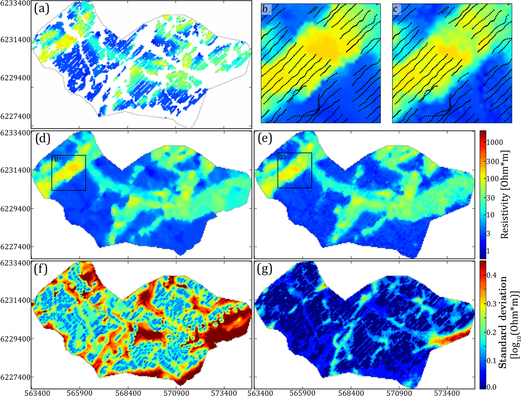
Figure 2 Comparison of the deterministic kriging and stochastic DS resistivity grid reconstruction and their corresponding standard deviation. The presented horizontal slice is centered on 20 m b.s.l. (a) shows the incomplete resistivity grid using simple kriging with a kriging radius of 50 m, (b) shows a close-up of the reconstructed resistivity grid using kriging, (c) shows a close-up of the reconstructed resistivity grid (shown in e) using DS, (d) shows the full reconstructed resistivity grid using kriging, (e) shows a single realization of the full reconstructed resistivity grid using DS, (f) shows the standard deviation from the reconstructed resistivity grids of (d) using kriging, and (g) shows the standard deviation calculated from an ensemble of 51 stochastic reconstructed resistivity grids using DS.

It is important to note that the resistivity parameter uncertainty has neither been included in the kriging nor the DS reconstruction, enabling the comparison of the SD maps. As an example, a gap present in the homogeneous conductive units with resistivity values between ∼ 2 and 8 Ω⋅m has a low SD. According to the TI there is a high probability of finding a conductive unit in a gap surrounded by only conductive units due to the homogeneity of such conductive units. However, gaps fringing the border of two contrasting resistivities have large SD values, since information regarding the exact location of the boundary is missing in the TI (e.g., the large SD value at the eastern border of the survey area seen in Fig. 2g).

In summary, the uncertainty of the DS reconstruction provides additional information regarding the reconstructed resistivity patterns over, for instance, a kriging approach. Also, the MPS reconstruction of the incomplete dataset is less smooth, easier to parameterize, and stochastic, and the uncertainty is related to pattern reconstruction and not the distance to the nearest data point.

3.3 Hydrostratigraphic modeling setup

The MPS grid reconstruction procedure is used to generate an ensemble of resistivity grids without gaps (Mariethoz and Renard, 2010). The reconstructed resistivity grids are used as soft data for constraining the simulation of the hydrostratigraphic models, with the cognitive 3-D hydrostratigraphic model used as a TI. The full cognitive geological model contains a total of 42 different geological units (Høyer et al., 2015a), which have been grouped together to form three key hydrostratigraphic categories. The three categories are described as follows.

1. Sand and gravel: Miocene sand, Quaternary meltwater sand and sand till, within and above the Quaternary buried valleys.

2. Glacial clay: Quaternary clay till and meltwater clay within and above the buried valleys.

3. Hemipelagic clay: hemipelagic, fine-grained Paleogene and Oligocene clays.

The simplified cognitive hydrostratigraphic model is used as a TI and contains the most significant hydrostratigraphic units. Such 3-D voxel TIs are usually not readily available, and in most cases 3-D TIs are fabricated ad hoc and are merely conceptual. However, in this case the TI is actually the model we wish to simulate. The justification for this choice of TI lies in that this study is a proof-of-concept study, where three different MPS methods are compared against each other. Using a detailed TI containing the desired hydrostratigraphic concepts showcases how well the MPS methods perform in a stochastic hydrostratigraphic modeling workflow with a relevant TI.

The overall workflow can be seen in Fig. 3. In detail, the steps are described as follows.

1. The SkyTEM resistivity grids are reconstructed using the methodology of Mariethoz and Renard (2010) as described in Sect. 3.2 “Reconstructing incomplete dense geophysical datasets”.

2. The ensemble of reconstructed SkyTEM resistivity grids is used as soft data for constraining the three MPS methods.

   • a.

     A reconstructed resistivity grid and the TI are used in the snesim framework.

     • Using histograms created using the resistivity atlas approach presented by Barfod et al. (2016) (Fig. 4c and d) a single reconstructed resistivity grid is translated into a set of probability maps (Fig. 5).

     • The TI is used for conditioning in conjunction with the probability maps, which are used for spatially constraining the snesim simulations using the tau model (Journel, 2002). The end result is a realization of a hydrostratigraphic model.

   • b.

     A reconstructed resistivity grid is selected and used in combination with the TI for running DS.

     • The soft data variable (the resistivity grid) is used for both constraining and as the auxiliary variable. The soft data grid is directly available as an auxiliary variable since it geographically overlaps with the categorical TI variable. The combination of the cognitive hydrostratigraphic model and auxiliary variable creates a bivariate TI.

     • The bivariate TI is used together with the soft data grid to simulate a realization of the hydrostratigraphic model.

   • c.

     A reconstructed resistivity grid is used together with the TI for running iqsim.

     • As with DS, the soft data grid is used as an auxiliary variable and for spatially constraining the simulations. The TI and auxiliary variable are combined into a bivariate TI.

     • The bivariate TI is used to create a simulation of the hydrostratigraphic model.

Steps 2a–c are repeated N times, once for each reconstructed resistivity grid. In this study N= 51. For each of the 51 reconstructed soft data grids three simulations have been run – one simulation per MPS method (snesim, DS and iqsim), yielding a total of 153 hydrostratigraphic realizations.

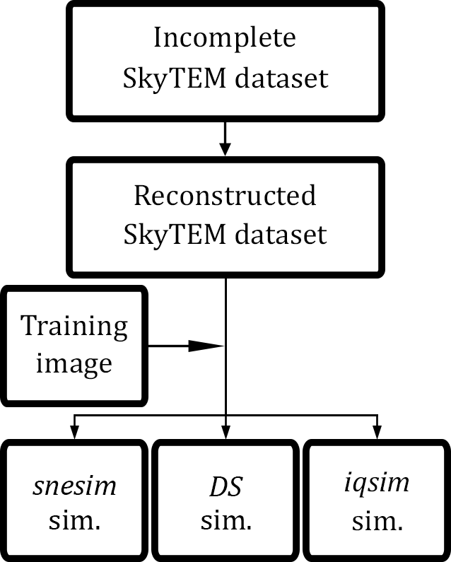
Figure 3 Workflow diagram showing the stochastic modeling procedure for a single realization. Each simulation is run with snesim, DS and iqsim.

3.4 The hydrostratigraphic–resistivity relationship

Spatially constraining the simulations to the soft data requires information regarding the relationship between hydrostratigraphic units and, in this case, resistivity values. In DS and iqsim the information is contained in the bivariate TI, which in this case consists of a categorical and a continuous auxiliary variable. As discussed in Sect. 3.1.2 the setup used in this paper avoids using the G^∗ operator due to the geographically overlapping resistivity and cognitive hydrostratigraphic model grids. This also enables summarizing the hydrostratigraphic–resistivity relationship as a set of histograms (Fig. 4a and b). The histograms summarizing the hydrostratigraphic–resistivity relations used in DS and iqsim are seen in Fig. 4a, and the corresponding summary statistics are found in Table 1. These histograms are created by selecting one of the reconstructed resistivity grids and combining it with the TI. The same relationship is seen in Fig. 4b; however, instead of using the DS reconstructed resistivity grid the kriging reconstructed grid is used. The main difference between the two sets of histograms is a slightly larger separation of the sand and gravel and the glacial clay for the kriging reconstructed grid (Fig. 4a and b) (Table 1). For the DS reconstructed grid the median values for sand and gravel and glacial clay histograms are 48 and 32 Ω⋅m, respectively, while for the kriging reconstructed grid the median values are 46 and 27 Ω⋅m, respectively. Furthermore, the kriging sand and gravel histogram is wider with an interquartile range of 38 Ω⋅m, which for the DS grid was 31 Ω⋅m.

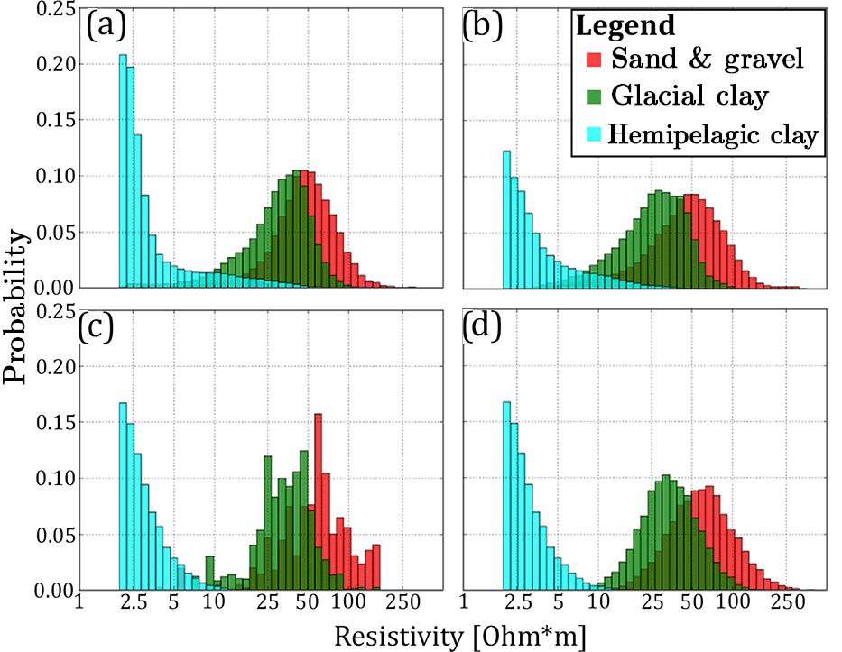
Figure 4 The hydrostratigraphic–resistivity relation shown as a series of histograms. (a) shows the histograms created by categorizing the DS reconstructed resistivity grid according to the simplified hydrostratigraphic model created by Høyer et al. (2015a), (b) shows the histograms created by categorizing a resistivity grid which has been reconstructed using kriging, (c) shows the histograms resulting from the resistivity atlas approach presented by Barfod et al. (2016), and (d) shows the resistivity atlas histograms that have been reproduced based on the summary statistics from (c) to create a set of lognormal histograms.

In the snesim framework, constraining to the soft data requires a translation of the soft resistivity data into a set of probability maps, one for each of the hydrostratigraphic units. This is achieved by using prior information regarding the hydrostratigraphic–resistivity relationship. Often this information is difficult to obtain, unless a large number of boreholes are available. If boreholes are readily available the resistivity atlas framework (Barfod et al., 2016) can be utilized. The raw resistivity atlas histograms are seen in Fig. 4c. Due to the general coarse nature of the histograms the mean and interquartile range from the coarse histograms (Fig. 4c) were computed and used to create a set of smooth histograms with identical summary statistics (Fig. 4d). By comparison the resistivity atlas histograms are quite similar to the kriging grid histograms (Fig. 4b). However, the separation between the (i) sand and gravel and (ii) glacial clay histograms is even larger in the resistivity atlas histograms. The respective median values are 59 and 34 Ω⋅m. The sand and gravel histogram also has a quite large spread with an interquartile range of 43 Ω⋅m (Fig. 4c and d) (Table 1).

Table 1 The summary statistics table for the histograms in Fig. 4. The first section, named DS, shows summary statistics for the three histograms seen in Fig. 4a. The second section, named kriging, shows the summary statistics for the histograms in Fig. 4b. The last section, labeled resistivity atlas, shows the summary statistics for the resistivity atlas histograms in Fig. 4c and d. All the values presented in the table are resistivities (Ω⋅m).

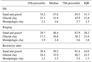
The hemipelagic clays have unique properties. They are aquitards with low hydraulic conductivity and often used as a hydraulically confining no-flow boundary at the bottom of a groundwater model in parts of Denmark. When hemipelagic clay is encountered during drilling, the drilling is halted and generally hemipelagic clay is sparse in Danish borehole lithology logs. For this reason the resistivity atlas based on transient electromagnetic data does not provide a lot of information on hemipelagic clays. However, the hemipelagic clays are regionally extensive and homogeneous. From wireline resistivity logs in eastern Jutland they are found to be conductive, with median resistivities ranging between 4–7 Ω⋅m. Based on this knowledge the hemipelagic clay histograms in Fig. 4c and d are created.

The model setup is different for the three MPS methods. When running DS and iqsim the hydrostratigraphic–resistivity relationship is explicitly given due to the geographically overlapping resistivity grid and hydrostratigraphic TI. Normally the auxiliary variable has to be created for the given TI using the G^∗ operator. The full G^∗ approach has been elaborated in Sect. 3.1.2 and requires prior knowledge regarding the hydrostratigraphic–resistivity relationship, much like when creating the probability grid for snesim. The snesim setup, however, avoids using the G^∗ operator approach, and in place the resistivity atlas histograms (Fig. 4c and d) can be used to directly translate the resistivity grid into probability grids (Fig. 5).

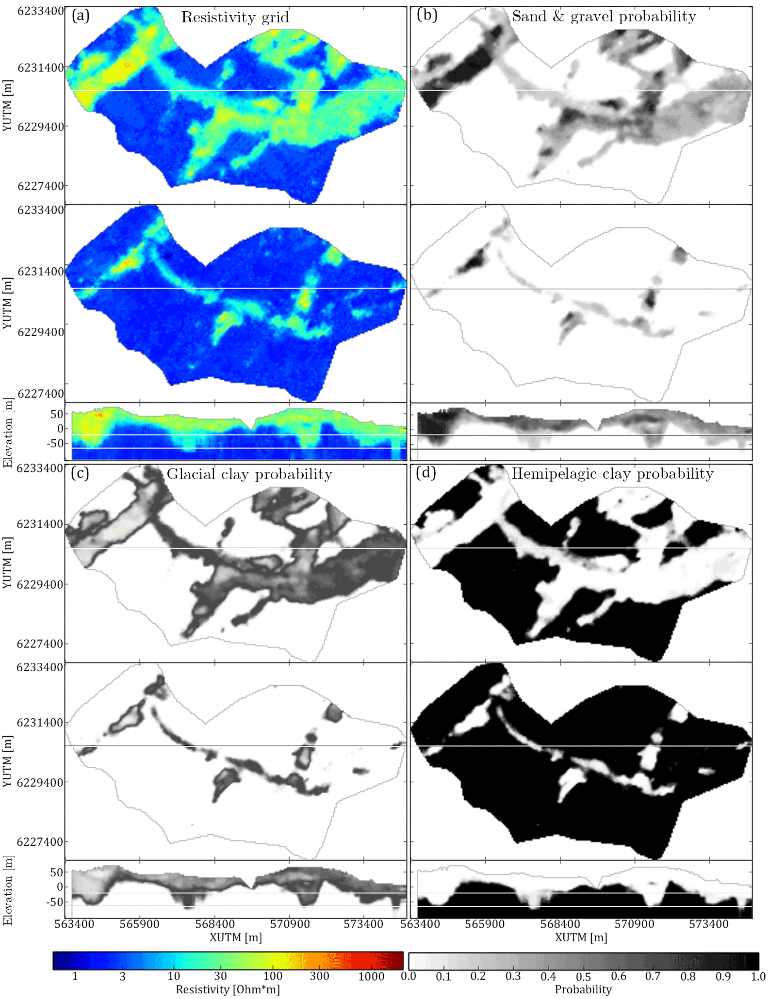
Figure 5 The SkyTEM soft data grids are translated into three sets of probability grids, one for each lithological category to be simulated; (a) shows one of the reconstructed SkyTEM grids – the top frame is a horizontal slice in the 3-D grid at 20 m b.s.l., the second frame is a horizontal slice of the grid layer at 60 m b.s.l. and the bottom frame shows the vertical cross section intersecting at UTMY coordinate 6 230 150 m; (b) shows the sand and gravel probability grid; (c) shows the glacial clay probability grid; and (d) shows the hemipelagic clay probability grid. The horizontal slices and the vertical cross sections of (b), (c) and (d) are the same as the ones presented in (a).

3.5 The modified Hausdorff distance – a measure for similarity

Comparing 153 3-D models each with 1 187 823 grid cells is not trivial. Visual comparison is used mainly to check if the results are geologically realistic, but a detailed visual comparison would be time consuming and subjective. Therefore, a set of tools are used to compare how similar the simulation results are to each other and how different they are from the TI.

In this study, a distance measure is used as a measure of similarity between 3-D model simulations. The chosen distance measure is the modified Hausdorff distance (D_MH), which is a measure for similarity between two binary images; i.e., dissimilar images have relatively large distances (Fig. 6e), while similar images have relatively small distances (Fig. 6c). Identical images have a distance of exactly zero (Fig. 6b). Firstly, the images we wish to study are summarized as binary images. The pixels for each object we wish to compare are set to one, while the remaining pixels are disregarded as a background variable and set to zero. For a pair of images, Im_A and Im_B, to be compared, two point sets are defined: $A=\left\{a_{\mathrm{1}},a_{\mathrm{2}},\mathrm{\dots },a_{N_a}\right\}$ and$B=\left\{b_{\mathrm{1}},b_{\mathrm{2}},\mathrm{\dots },b_{N_b}\right\}$, where $a_i,i\in \left\{\mathrm{1},\mathrm{2},\mathrm{\dots },N_a\right\}$ and $b_j,j\in \left\{\mathrm{1},\mathrm{2},\mathrm{\dots },N_b\right\}$ are positional vectors containing the x, y and z positional coordinates in Im_A and Im_B for the binary object pixels only; i.e., the background variable positions are not included in the point sets. Then the D_MH between point sets A and B is defined as follows:

$$\begin{array}{}\text{(2)}& D_{\mathrm{MH}}\left(A,B\right)=\max \left({\displaystyle \frac{\mathrm{1}}{N_a}}\sum _{a\mathit{ϵ}A}{\min }_{b\mathit{ϵ}B}∥a-b∥,{\displaystyle \frac{\mathrm{1}}{N_b}}\sum _{b\mathit{ϵ}B}{\min }_{a\mathit{ϵ}A}∥b-a∥\right),\end{array}$$

where N_a and N_b are the total number of points in point sets A and B, respectively. In the context of this paper, A and B are our 3-D voxel models containing the objects we wish to compare. The Euclidian distances between a given point a from point set A and all points in point set B are computed, and min(…) selects the smallest of these distances. This is repeated for all points in point set A, and the average is computed. The same operations are performed for point set B. The maximum value of these two results is then returned.

Dubuisson and Jain (1994) found that the D_MH was the best performing distance measure out of 24 different Hausdorff-based distance measures in relation to objects matching of images. In order to make the pairwise D_MH computation tractable in 3-D, we approximate the D_MH between solid geobodies by the D_MH between their boundaries. In short, the boundary is the selection of the edges or outlines of the geometric objects, such that the objects are now represented by their outlines instead of the entire objects (see Fig. 6b–e). The Roberts cross operator (Roberts, 1998; Senthilkumaran and Rajesh, 2009) is used to select the boundary. Instead of defining the point sets based on the geometric objects themselves, only their outlines are included in the point sets. The point sets containing the outline of the geometric objects are then compared using the D_MH.

A 2-D example is presented to illustrate the overall D_MH concept in Fig. 6. The 3-D hydrostratigraphic model and the DS modeling results are simplified into 2-D horizontal cross sections from the modeling grid layer centered on 20 m b.s.l. The initial step is to create a binary version of the hydrostratigraphic simulation model (Fig. 6a and b). Ideally, it would be optimal to compute the D_MH between each of the hydrostratigraphic categories of the model. However, due to computational limitations of the utilized D_MH implementation, the valley categories, i.e., sand and gravel and glacial clay, were re-categorized as a single unit, and hemipelagic clay was used as the background variable. After categorization, the Roberts cross operator is used to find the boundary of the objects (Fig. 6b). The procedure of creating the binary image and outlines is carried out for all the 51 DS simulations. For illustration purposes, this example is only computed for the horizontal cross section centered on 20 m b.s.l. The D_MH is calculated between each of the 51 horizontal binary maps, representing the DS simulations, and the binary hydrostratigraphic model. The resulting D_MH values are then sorted in ascending order and the binary version of the realizations corresponding to the 1st, 25th and 51st D_MH values are presented in Fig. 6c–e.

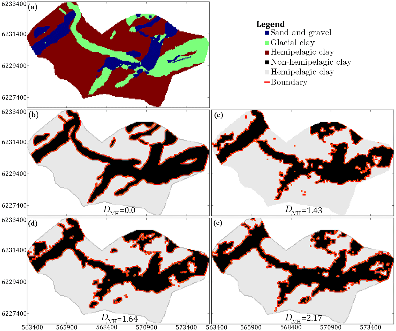
Figure 6 A 2-D example of the binary categorization of the hydrostratigraphic models and example of the Roberts cross operator for edge tracing. (a) a horizontal slice of the hydrostratigraphic model at elevation interval centered on 20 m b.s.l.; (b) the result of the binary categorization of the hydrostratigraphic model into two categories – (1) non-hemipelagic clay (black) and (2) hemipelagic clay (white). The boundary of the objects in the binary image is shown in red. (c) shows the object and boundary of the objects for the DS simulation which has the smallest modified Hausdorff distance (D_MH), i.e., it is the most similar to (b). (d) shows the DS simulation, which has the 25th largest D_MH; and (e) shows the DS simulation with the largest D_MH and therefore represents the model which is least similar to (b).

From here on, we leave the 2-D example and consider the entire 3-D model. In this study, the D_MH is used as a global distance measure. A more in-depth analysis of the D_MH results is gained by using the analysis of distance method (Tan et al., 2014). The overall goal of ANODI is to provide a framework for comparing realizations from different stochastic MPS methods. The framework presented by Tan et al. (2014) uses the following definition of “best”: “one algorithm A is better than an algorithm B if the training image statistics are reproduced better while at the same time the space of uncertainty (the variability between realizations) is larger”. In the particular MPS setup used in this study, the TI is a relevant cognitive hydrostratigraphic model and geographically overlaps with the hydrostratigraphic MPS realization grids. Hence, the MPS realizations should portray similarity to the cognitive model. In this study, a further complexity to the definition of best is added. An algorithm with a large space of uncertainty is not necessarily better if the resulting models do not reflect the underlying datasets.

The initial step is to create a matrix containing all D_MH values between all 153 realizations and between the individual realizations and the cognitive model. It is similar to a covariance matrix, but, instead of containing covariance values, it contains D_MH values. The usage of bold letters refers to a matrix. The full D_MH is computed as follows:

$$\begin{array}{}\text{(3)}& D_{\mathrm{MH}}^{(i,j)}=D_{\mathrm{MH}}\left({\mathrm{real}}_i,{\mathrm{real}}_j\right),\mathrm{where}\left\{\begin{array}{c}i=\mathrm{1},\mathrm{\dots },(N_{\mathrm{reals}}+\mathrm{1})\\ j=\mathrm{1},\mathrm{\dots },(N_{\mathrm{reals}}+\mathrm{1})\end{array}\right.,\end{array}$$

where $D_{\mathrm{MH}}^{(\mathrm{i},\mathrm{j})}$ denotes the D_MH at position (i,j) of the D_MH matrix; real_i and real_j denote the individual hydrostratigraphic realizations; N_reals is the total number of realizations, in this case N_reals=153; and the last row and column of D_MH contains the distances between the realizations and the cognitive model – i.e., real${}_{N_{\mathrm{reals}}+\mathrm{1}}$ represents the cognitive model. One D_MH matrix is created for all three MPS methods. For each of the three MPS methods, the D_MH can be evaluated by itself by calculating the D_MH variability, D_MH, var:

$$\begin{array}{}\text{(4)}& D_{\mathrm{MH},\mathrm{var}}={\displaystyle \frac{\mathrm{1}}{{\left(N_{\mathrm{reals}}/\mathrm{3}\right)}^{\mathrm{2}}}}{\sum }_{i={\mathrm{MPS}}_{\mathrm{start},i}}^{{\mathrm{MPS}}_{\mathrm{end},i}}{\sum }_{j={\mathrm{MPS}}_{\mathrm{start},j}}^{{\mathrm{MPS}}_{\mathrm{end},j}}\left(D_{\mathrm{MH}}^{(i,j)}\right),\end{array}$$

where N_reals is the size of D_MH (in this study $N_{\mathrm{reals}}=\mathrm{3}\times \mathrm{51}=\mathrm{153}$), MPS_start,i and MPS_end,i are the start and end indexes for the entries related to the given MPS method, and ${\mathrm{D}}_{\mathrm{MH}}^{(i,j)}$ is D_MH(real_i,real_j). Note that the distances between the individual realizations and the cognitive model are not included in the D_MH,var. The D_MH,var equates to computing the average of the D_MH values between the realizations of a single MPS method. The larger the D_MH, var, the more dissimilar the simulation results, meaning they portray a large set of possible hydrostratigraphic architectures. Using Eq. (4) it is also possible to compute the distances between the realizations of different MPS methods, e.g., the average D_MH between snesim and DS.

The other evaluation measure, which can be calculated from D_MH, is the distance between the realizations and the cognitive hydrostratigraphic model (cog), or TI, which is summarized by the D_MH,cog, which is computed as follows:

$$\begin{array}{}\text{(5)}& D_{\mathrm{MH},\mathrm{cog}}={\displaystyle \frac{\mathrm{1}}{N_{\mathrm{reals}}/\mathrm{3}}}{\sum }_{i={\mathrm{MPS}}_{\mathrm{start},i}}^{{\mathrm{MPS}}_{\mathrm{end},i}}\left(D_{\mathrm{MH}}^{(i,N_{\mathrm{real}}+\mathrm{1})}\right),\end{array}$$

where, again, N_reals=153, MPS_start,i and MPS_end,i are the start and end indexes for the entries related to the given MPS method and $D_{\mathrm{MH}}^{(i,N_{\mathrm{real}}+\mathrm{1})}$ is the D_MH(real_i,cog). The D_MH,cog is the average D_MH between each individual realization and the cognitive hydrostratigraphic model. The larger the average D_MH, the more dissimilar the hydrostratigraphic realizations are from the cognitive hydrostratigraphic model. The reason we wish to compare the distance to the cognitive model is that the cognitive model geographically overlaps with the hydrostratigraphic MPS realizations.

It is also possible to evaluate the D_MH using dimensional reduction techniques. Such techniques help us view the high dimensional D_MH in a 2-D and/or 3-D map. Such a plot gives us a visual representation of the most significant structures of the D_MH. For dimensional reduction we use a variation of so-called stochastic neighbor embedding (SNE) (Hinton and Roweis, 2002). The technique is called t-distributed stochastic neighbor embedding, or t-SNE (Maaten and Hinton, 2008). The t-SNE method is advantageous over other SNE techniques, since it is easier to optimize and produces better visualizations. The idea is to visualize the level of similarity of individual entries, or distances in the D_MH. The overall goal is to place each D_MH value as a point in a 2-D space where the relative distances between the point values reflect the degree of similarity. Similar points are close to each other, while dissimilar points are far from each other. This is achieved by t-SNE.

3.6 Distance to boreholes

In reservoir modeling, boreholes are considered to be hard information, due to their overall high quality. However, in many surveys related to groundwater modeling, boreholes cannot be considered as reliable hard data due to variable quality – such as seen in Barfod et al. (2016) and He et al. (2014), where boreholes were divided into quality groups. Therefore, the simulations are run without constraining against boreholes, and then the realizations are compared against the boreholes as an independent measure of geological realism. A method for comparing similarity between the simulated hydrostratigraphic models and the boreholes was developed. The method does not use the D_MH, which has previously been used for measuring distances. Instead, the simple Euclidean distance is used to measure the average distance between each individual hydrostratigraphic realization and the borehole dataset. The first step is to sort the borehole lithology logs according to the respective hydrostratigraphic units to create a hydrostratigraphic log (see left half of Fig. 7). Once this has been carried out, three sets of binary and regularized logs are created from the hydrostratigraphic log (see right half of Fig. 7). For each sampling grid interval, the presence of the given hydrostratigraphic category, say sand and gravel, is saved in the binary log. The end result is a log which states whether or not sand and gravel is present within the given sampling grid interval – active if present and inactive if not present. Three such binary logs are created, one for each of the hydrostratigraphic categories, i.e., sand and gravel, glacial clay and hemipelagic clay (Fig. 7). A binary log grid is created by simply assigning the binary active values to the grid cell in which they are present. The average Euclidian borehole distance, D_AEB, between the binary logs and a given realization (real) for a given hydrostratigraphic category (hydro. cat_j, where $j\in \left\{\mathrm{1},\mathrm{\dots },N_{\mathrm{hydro}.\mathrm{cats}}\right\}$), is calculated as follows:

$$\begin{array}{ll}{\displaystyle }{D}_{\mathrm{AEB}}\left(\mathrm{hydro}.{\mathrm{cat}}_j\right)& {\displaystyle }={\displaystyle \frac{\mathrm{1}}{N_{\mathrm{active}}}}{\sum }_{i=\mathrm{1}}^{N_{\mathrm{active}}}\\ \text{(6)}& {\displaystyle }& {\displaystyle }\left(∥{\mathrm{binlog}}_i-\mathrm{real}(\mathrm{hydro}.{\mathrm{unit}}_j)∥\right),\end{array}$$

where binlog_i is ith active cell in the binary log grid; N_active is the number of active cells in the binary log grid; ED is the Euclidian distance; and real(hydro. unit_j) is the binary realization grid containing only the jth hydrostratigraphic unit, where in this case $N_{\mathrm{hydro}.\mathrm{cats}}=\mathrm{3}$.

The end result is three arrays, one for each hydrostratigraphic unit, each containing one average distance per realization for the given MPS method. The distance arrays for each individual MPS method can then be compared to the distance arrays of the other MPS methods.

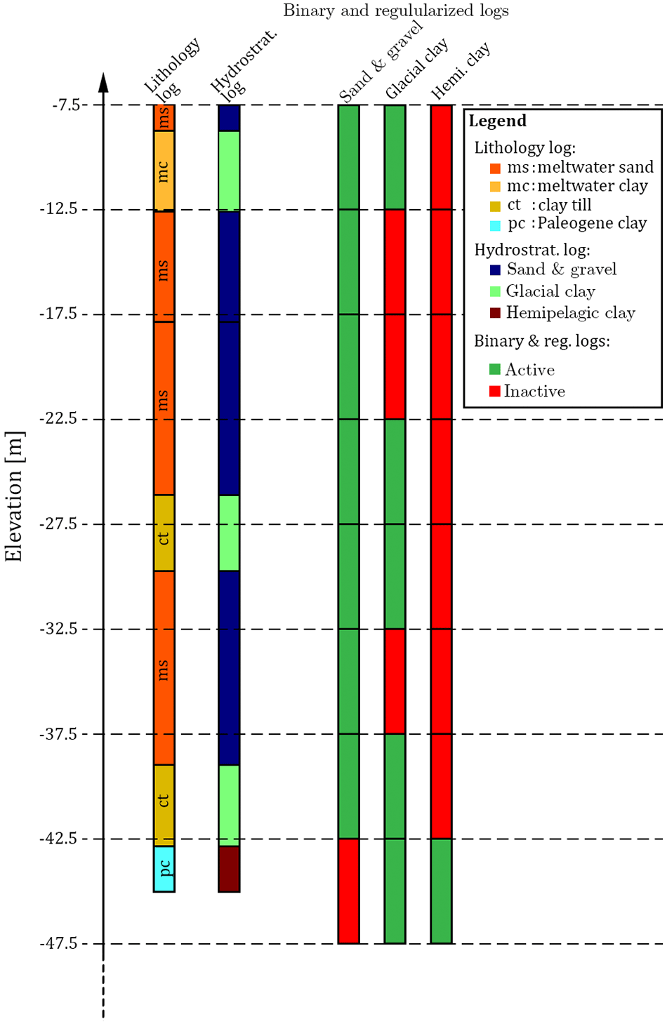
Figure 7 An example of how a single lithology log is categorized and sorted for the purpose of calculating the borehole distance. The first step is to translate the raw lithology log into a hydrostratigraphic log, which is achieved by categorizing the multiple lithological categories into a subset of three hydrostratigraphic categories corresponding to the target categories we wish to model. Note that some categories do not fit into the overall hydrostratigraphic categories and are therefore not translated, e.g., the meltwater sand category in this example. The final step is then to assign the hydrostratigraphic logs to the regularized sampling grid and create one binary log for each of the three target modeling categories. This is done by simply asking whether or not the given hydrostratigraphic category is present (true) or not (false) for the given sampling grid interval.

4 Results

The hydrostratigraphic simulation results include 153 3-D hydrostratigraphic realizations, each containing 1 187 823 grid cells. The models can be subdivided into 51 snesim realizations, 51 DS realizations and 51 iqsim realizations. A visual presentation of the hydrostratigraphic model or TI as well as two realizations for each of the three different MPS methods is seen in Fig. 8. The cognitive hydrostratigraphic model (Fig. 8a) shows clear-cut and smooth buried valley architecture with almost no short-scale variability. Comparing the cognitive hydrostratigraphic model to the stochastic MPS hydrostratigraphic models reveals the more erratic nature of both snesim and DS; i.e., both MPS methods yield models containing short-scale variability (Fig. 8b and c).

Overall snesim (Fig. 8b) and DS (Fig. 8c) realizations are similar in nature. In the example provided, Fig. 8c, the west–northwest- to east–southeast-trending glacial clay valley (see box in Fig. 8a) is uninterrupted in one realization, but intersected by hemipelagic clay in the other realization. In 47 of the 51 snesim realizations, the glacial clay valley is uninterrupted; in the remaining 4 realizations the valley is intersected by hemipelagic clay. The presented soft data grid in Fig. 5d shows a small probability of approximately 10 % for hemipelagic clay at the position of the valley gap. The 4 realizations which yielded an interrupted glacial clay valley amount to 8 % of the 51 realizations, which is close to the probability found in the probability grids. The DS realizations shows valley architecture with less resemblance to the soft data, i.e., the valleys are not conditioned in accordance to the soft data grids. In 11 of the 51 simulation results the valley is intersected by hemipelagic clay, amounting to 22 % of the 51 realizations.

The iqsim results are the most similar to the cognitive hydrostratigraphic model with regards to short-scale variability, which is generally nonexistent. Generally, realizations will reflect the TI, and short-scale variability is only introduced if present in the TI. This is due to the nature of iqsim, which is not a pixel-based algorithm, like snesim and DS. Instead, iqsim cuts the TI into patches and then reassembles the patches, which means that noise patterns which are smaller than the patch size cannot be fabricated, unless actually present in the TI. The iqsim realizations show smooth and clear-cut valley architecture. The main issue with the iqsim realizations is that artifacts are introduced near the surface of the model, which is evident if the vertical iqsim cross sections (Fig. 8d) are compared to the remaining vertical cross sections of the TI, snesim and DS (Fig. 8a–c). This is neither reflected in the resistivity grid (Fig. 5) nor in the TI (Fig. 8a). Close to terrain hydrostratigraphic layers consist of either glacial clays or sand and gravel, and conductive hemipelagic clays are not evident. Since the soft data does not support the presence of the hemipelagic clays in the upper part of the hydrostratigraphic model, the soft data can be concluded to be improperly constrained with this specific setup. Another observation is that in 43 out of the 51 realizations, amounting to 84 %, the referenced glacial clay valley is intersected by hemipelagic clay.

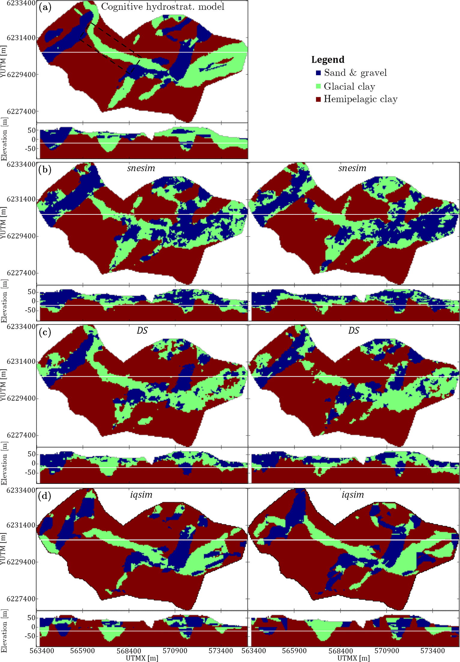
Figure 8 The hydrostratigraphic MPS realizations are presented as horizontal slices centered on 20 m b.s.l. and vertical cross sections intersecting at UTMY 6 230 150 m. (a) shows the cognitive hydrostratigraphic model, with a west–northwest- to east–southeast-trending glacial clay valley marked by a box; (b) shows two snesim realizations; (c) shows two DS realizations; and (d) shows two iqsim realizations.

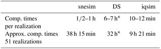
An advantage of the iqsim implementation used (Hoffimann et al., 2017) is the favorable computation time. On an Intel®HD Graphics Skylake ULT GT2 GPU of a Dell XPS 13 laptop, iqsim runs with an average simulation time of 10–12 min per realization with the attempted setup. On a different laptop running a 64 bit Windows system, with 8 GB RAM, an SSD hard disk, with an Intel®Core i7-3520 M CPU at 2.9 GHz, the computation times for snesim were on average between 1∕2 and 1 h. Since the DS computation times were significantly larger at 6 h 15 min per realization, the DS simulations were run on a 64 bit Windows server with a 64 bit AMD Opteron processor 5376 at 2.3 GHz each, with a total of 128 GB RAM and a SSD hard disk. The implementation of DS used in this paper is called DeeSse (Straubhaar, 2011) and is easy to script and run in parallel on a server or computer cluster. The total time required for 51 simulations running in parallel was approximately 32 h, without enabling parallelization, which is available in DeeSse. One DS simulation took between 6 and 7 h. For more detailed information see Table 2, which summarizes computation times for the three MPS methods.

Table 2 A table presenting the average computation times per realization for each of the three MPS methods and the approximated computation times needed for running 51 realizations with the setup used in this study. ^* indicates that the given realizations were run in parallel on a server; other realizations were generated on a personal laptop.

4.1 Modified Hausdorff distance results

The D_MH is computed for a binary case where the glacial clay and sand and gravel have been combined into one category. Therefore, the D_MH measures differences in the overall buried valley architecture. The full D_MH matrix is presented in Fig. 9a and b. Using Eqs. (4) and (5) the D_MH is summarized in Table 3, without the usage of dimensional reduction techniques. The method with the largest variability, i.e., least similar hydrostratigraphic realizations, is iqsim, with a D_MH,var of 1.79. The snesim and DS models show generally lower D_MH,var values of 0.48 and 0.78, respectively. This means that the iqsim results span the largest set of possible models, when measuring on the binary classification in hemipelagic clay and not hemipelagic clay. The iqsim realizations also have the smallest average D_MH between the individual realizations and the cognitive hydrostratigraphic model, with a D_MH,cog of 2.65, meaning that on average iqsim realizations resemble the cognitive hydrostratigraphic model the most, when it comes to the location of the valleys. The snesim and DS D_MH,cog are 3.01 and 2.80, respectively. On average, the DS realizations are more similar to the cognitive hydrostratigraphic model in comparison to the snesim realizations, while both are more dissimilar than the iqsim realizations – again, when it comes to the location of the valleys. The two MPS methods which had the smallest distances, and therefore were most similar, were snesim and DS, with an inter D_MH distance of 1.05. The distance between DS and iqsim was larger, with a value of 2.19, while the largest inter D_MH distance was between snesim and iqsim with a D_MH value 2.37.

Table 3 Summary of the modified Hausdorff distance (D_MH) matrix portraying the D_MH results. D_MH,var presents the variability of the given MPS method or between the different MPS methods; for example, the value in the D_MH,var column and the snesim → DS row represents the average distance between the snesim and DS realizations. The D_MH,cog is the average distance from the simulation results to the cognitive model.

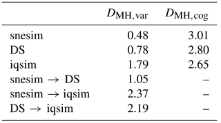
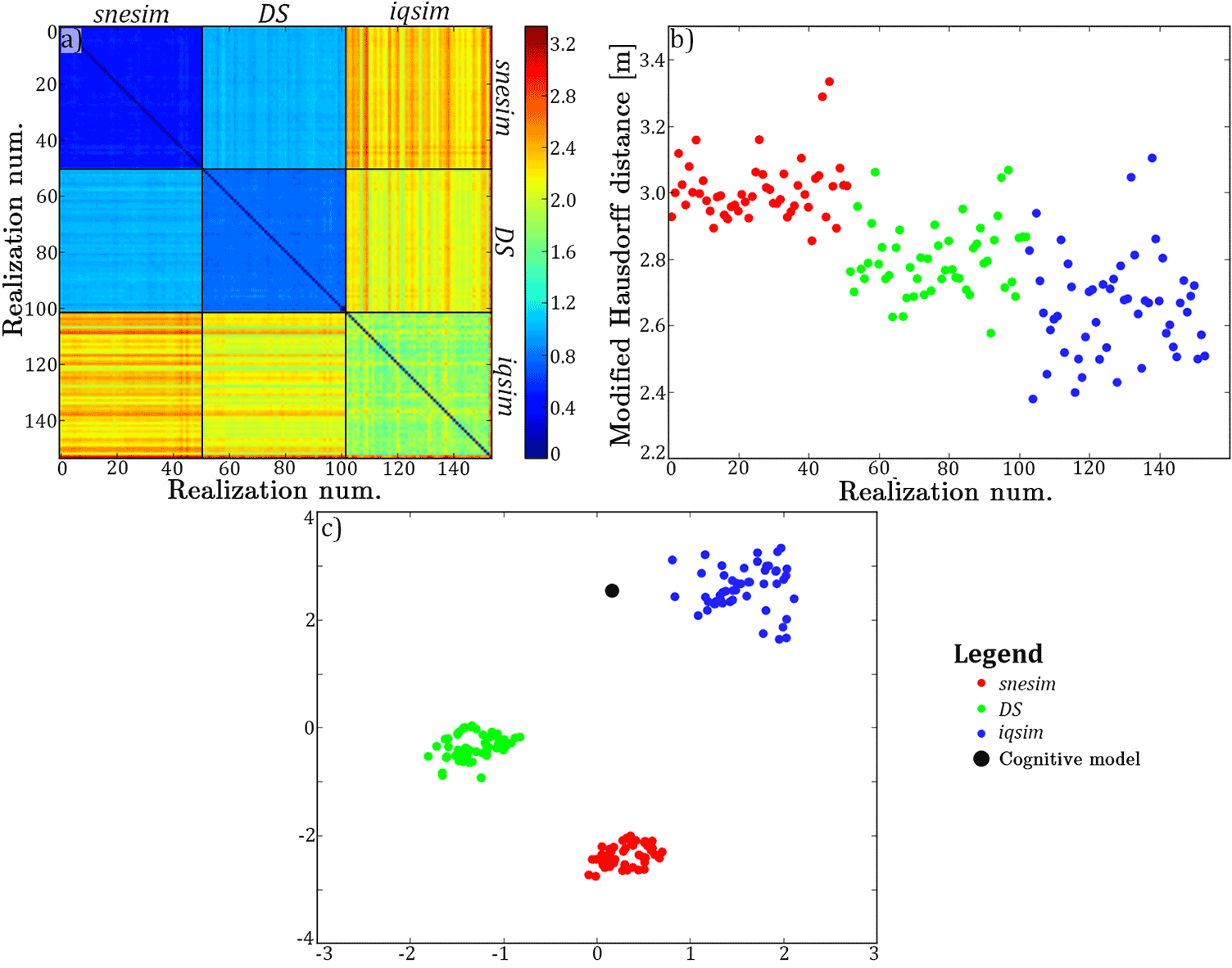
Figure 9 The D_MH results presented without and with dimensional reduction. (a) The full modified Hausdorff distance (D_MH) matrix showing the distances between individual realizations and between individual realizations and the cognitive hydrostratigraphic model. The last column and row of the distance matrix of (a) represent the distances between the realizations and the cognitive model. (b) shows a scatterplot of these distances between the realizations and the cognitive model, revealing greater detail than can be seen with the naked eye from the D_MH matrix itself. (c) shows the 2-D t-SNE plot of the D_MH matrix.

The D_MH can also be evaluated by applying the aforementioned t-SNE method. Here, each realization is visually represented as a point in 2-D space. Similar values, with small D_MH values, are closely spaced, while dissimilar values, with large D_MH values, are separated from each other. Firstly, the t-SNE results show snesim and DS point clouds, which are closer to each other relative to the iqsim point cloud (Fig. 9c). This means that they are similar in nature, as reflected in Table 3. The iqsim point cloud is isolated in the 2-D space since the iqsim realizations are significantly different from the snesim and DS results. Furthermore, the iqsim point cloud is also the largest, which reflects the larger dissimilarity of the output realizations. On average, the iqsim point cloud is closer to the cognitive model, which is also reflected in Fig. 9b and Table 3.

4.2 Borehole validation results

The final comparison of the MPS methods regards the average Euclidean distance between the simulation results and the regularized binary hydrostratigraphic logs. The sorted average distances between each individual simulation and the boreholes are seen in Fig. 10.

Figure 10 The borehole distance results are presented for each of the three MPS methods: snesim, DS and iqsim. (a) shows the snesim borehole distance results for the three hydrostratigraphic units, (b) shows the DS borehole distance results for the three hydrostratigraphic units, and (c) shows the iqsim borehole distance results for the three hydrostratigraphic units.

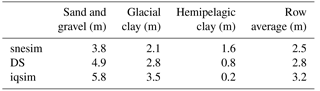
The average distances between the simulated hydrostratigraphic models and the boreholes are presented according to the three key hydrostratigraphic units. The average distance between sand and gravel units in the hydrostratigraphic realizations and sand and gravel units in the boreholes seems to be the largest for the modeling results of all three MPS methods (Fig. 10); i.e., the red curve is always on top. The average values of the individual curves in Fig. 10 are computed and presented in Table 4. An overall borehole distance average for each of the three MPS methods is computed as the average of each row in Table 4. The sand and gravel average in Table 4 reflects the large distances between resistive sand and gravel units in the realizations and the hydrostratigraphic logs. By comparing the individual frames of Fig. 10 it is seen that the average values for the hydrostratigraphic models created using iqsim have a higher average distance. The iqsim average for sand and gravel is centered on 5.8 m, while for snesim and DS it is centered on 3.8 and 4.9 m, respectively. The iqsim average distance to glacial clay is centered on a relatively large value of 3.5 m, as opposed to 2.1 and 2.8 m for snesim and DS, respectively. The hemipelagic clay units show a different pattern where iqsim has the lowest average distance of 0.2 m, while the snesim and DS distances are 1.6 and 0.8 m, respectively. The snesim method has the smallest borehole distance row average of 2.5 m, while DS and iqsim have row averages of 2.8 and 3.2 m, respectively.

Table 4 The borehole distance results are summarized in this table. The borehole distances are the 3-D Euclidean distances calculated using the concept presented in Sect. 3.6. The presented distance values are the averages of the curves shown in Fig. 10, one average for each of the individual hydrostratigraphic units for each of the presented methods: snesim, DS and iqsim realizations. The last column shows the average distances for each of the three MPS methods.

4.3 Hydrostratigraphic modeling of new surveys

In areas of groundwater interest, the initial step is to collect different types of data relevant to the hydrogeological properties of the subsurface. Among these data are dense geophysical datasets, e.g., SkyTEM, which can be collected quickly and usually cover a significant part of the survey area. The different datasets are processed and modeled and used in conjunction with the borehole lithology logs to create a single geological and/or hydrostratigraphic model. This model is only one version of the subsurface, encasing only part of the complexity related to the given hydrological system. We present an example of stochastic simulation of hydrostratigraphic models. The result consists of multiple hydrostratigraphic realizations, covering a larger span of possible models. Using the cognitive hydrostratigraphic model from area A as a TI, another hydrostratigraphic model from survey area B is simulated, using only the geophysical data in area B for spatial constraining. An important assumption is that the geological settings of area A and B are similar, since the hydrostratigraphic information is shared through the TI from area A. Furthermore, the hydrostratigraphic–resistivity relationship needs to be stationary so that it can be assumed that the hydrostratigraphic–resistivity relationships are statistically comparable.

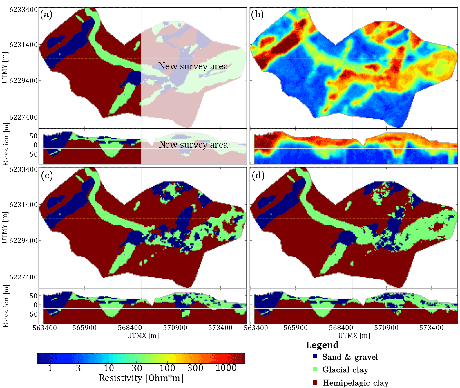
Figure 11 An overview of the setup for simulating new survey areas and the hydrostratigraphic modeling results using the Kasted dataset. The presented horizontal slices are centered on 20 m b.s.l., and the vertical cross section intersects at UTMY 6 230 150 m. (a) The cognitive hydrostratigraphic model is cut in half to simulate having two survey areas, one area with a cognitive hydrostratigraphic model (training image) available and the other without. The white area represents the new survey we wish to simulate. (b) The horizontal slices and vertical cross sections of the soft data used to simulate the new area. The left half is the auxiliary variable, while the right half constrains the simulation of the new survey area. (c) A single hydrostratigraphic realization. The left half is exactly the same as the cognitive model, see (a), while the right half is simulated using DS. (d) The mode of an ensemble of 10 hydrostratigraphic model realizations. Again, the left haft is the same as the training image and the right half shows the ensemble mode of 10 realizations.

The example presented in this study is synthesized from the Kasted dataset. The dataset is divided in two along the UTMX coordinate 569 025 m (Fig. 11a). The left half of the cognitive hydrostratigraphic model is then used as a TI to simulate the right half of the model. The reconstructed resistivity grid is also cut in half (Fig. 11b). The left half of the resistivity grid is used as an auxiliary variable describing the hydrostratigraphic–resistivity relationship, as seen in Fig. 4a, while the right half is used for spatially constraining the simulation. In this example 10 stochastic hydrostratigraphic realizations are created using DS. The DS method was selected since it is both easy to parameterize and to run in parallel on a computer cluster. A single hydrostratigraphic realization is seen in Fig. 11c, while the mode of the hydrostratigraphic model ensemble is seen in Fig. 11d. Using the same splitting of data and TI from the Kasted survey area, simulations using iqsim are presented by Hoffimann et al. (2017).

The simulation results show that one hydrostratigraphic realization represents the overall architecture of the resistivity grid (compare Fig. 11c and b). Comparing the single hydrostratigraphic realization (Fig. 11c) to the original cognitive model (Fig. 11a) reveals that one realization largely reflects the variability in the soft data grid. The mode of the model ensemble on the other hand (Fig. 11d) has a closer resemblance to the cognitive hydrostratigraphic model (compare Fig. 11a and d). This means that the individual realizations do on average resemble the original cognitive model. The end goal is not to create a set of hydrostratigraphic models which match the cognitive hydrostratigraphic model. The goal is to create a suite of realistic hydrostratigraphic models. Generally, short-scale variability is introduced in both the single hydrostratigraphic realization and in the ensemble mode model, but is generally not present in either the TI or the resistivity grid.

5 Discussion

The snesim setup is different from the DS and iqsim setups. The snesim setup differs in the usage of the probability framework and in the choice of the implicit resistivity atlas histograms (Barfod et al., 2016). The implicit histograms (Fig. 4d) are used to directly translate the resistivity grids into probability grids. This illustrates the utility of the resistivity atlas framework in relation to geostatistical modeling. The DS and iqsim frameworks would normally, in real-world cases, require the usage of a G^∗ operator since no auxiliary variable which geographically overlaps with a conceptual TI exists. As explained in Sect. 3.1.2, applying a realistic G^∗ operator requires several steps and can be a complicated affair. In this study, however, the TI was an actual cognitive geological model of the Kasted study area, meaning a resistivity grid which geographically overlaps with the TI exists. Using the SkyTEM resistivity grid as an auxiliary variable resulted in the application of different resistivity–hydrostratigraphic relationships in the DS and iqsim approach – compare the explicit histograms used in DS and iqsim, Fig. 4a, with the implicit resistivity atlas histograms used in snesim, Fig. 4d, or see Table 1. Even though there are some differences in the setups of the different MPS algorithms, the snesim and DS realizations are still similar in nature (compare Fig. 8b and c). The differences mentioned here are mainly due to the differences of the implementation of the algorithms.

The snesim and DS realizations portray some differences, which are related to the choice of the implicit resistivity atlas histograms for translating the resistivity grid. This can help us understand some of the basic differences in the information provided by the implicit resistivity atlas histograms and the explicit auxiliary variable. In DS probable hydrostratigraphic units are not conditioned properly. An example of this is the aforementioned west–northwest- to east–southeast-trending glacial clay valley (see Fig. 8a), which is uninterrupted in 78 % of the DS realizations. The same valley is clearly represented in the resistivity grid (Fig. 5a) and in the cognitive model (Fig. 8a). However, the explicit auxiliary variable histograms show increased overlapping resistivity values for the glacial clay and sand and gravel histograms (Fig. 4a, d). The auxiliary variable histograms (Fig. 4a) reveal approximately equal probability of glacial clay and sand and gravel resistivities lying close to 40–45 Ω⋅m. The histogram also shows that hemipelagic clay has a resistive tail, resulting in a small probability for hemipelagic clay in the areas of intermediate resistivity values of 10–50 Ω⋅m. The resistivity atlas histograms (Fig. 4d), on the other hand, favor the glacial clay in the 40–45 Ω⋅m range, with a 0 % probability for hemipelagic clay. The snesim realizations show an uninterrupted glacial clay valley in ∼ 90 % of the realizations in the horizontal cross section centered on 20 m b.s.l. The probability grid for snesim reveals a ∼ 75% probability for glacial clay at the location of the west–northwest- to east–southeast-trending glacial clay valley at 20 m b.s.l. (Fig. 5c). At 20 m b.s.l. sand and gravel has probability ∼ 15–20 %, while hemipelagic clay has a low probability of ∼ 0–5 % (Fig. 5b, d). The underlying hydrostratigraphic–petrophysical relationship, which holds information on how to condition the simulations to the soft data, is important to the MPS modeling results, especially when extensive and spatially dense geophysical datasets are available. The presented practical example, showing the simulation of a new survey, has the two aforementioned requirements: (1) the geological environments of the two areas need to be similar and (2) the statistical hydrostratigraphic–petrophysical relations also need to be similar. Since the resistivity atlas histograms are created using only local data, i.e., boreholes and SkyTEM resistivity models, they represent the local relationship. Since stationarity in the hydrostratigraphic–petrophysical relations is not guaranteed (Barfod et al., 2016), it is necessary to check for stationarity, which is possible within the resistivity atlas framework. Here, histograms can be created for each area and compared. If statistically similar, stationarity can be inferred for the hydrostratigraphic–petrophysical relations.

The D_MH results revealed some interesting trends between the MPS realizations. The D_MH,var for snesim, DS and iqsim were 0.48, 0.78 and 1.79, respectively. The low snesim D_MH,var is related to the soft data conditioning, which is dependent on the choice of histograms for translating the resistivity grids into probability grids. For this translation, as mentioned, the implicit resistivity atlas histograms were used. Overall, the implicit histograms show a larger separation between the glacial clay and hemipelagic clay histograms compared to the explicit histograms (compare Fig. 4a and d). This results in less ambiguity in the transition from glacial clay to hemipelagic clay in the probability grids, yielding a smaller subset of possible models. This also results in snesim realizations, which closely resemble the soft data variable, compared to DS and iqsim. The borehole distance results are also influenced by choosing the implicit histograms. Generally, the snesim realizations show the smallest borehole distances with respect to glacial clay and sand and gravel units, while the corresponding hemipelagic clay distances are the largest. The increased separation of the glacial clay and hemipelagic clay histograms seems to improve the snesim borehole distances to the glacial clay and sand and gravel units, while hemipelagic clay seems to be underestimated.

In conclusion, snesim and DS yield similar realizations, portrayed by the relatively small D_MH values between snesim and DS. This is reflected in the t-SNE plot (Fig. 9c), where the iqsim point cloud is isolated from the snesim and DS point clouds and is closer to the cognitive model. The isolation of the iqsim point cloud agrees with iqsim being imprecise in its simulation of the valley architecture compared to snesim and DS. However, the abundance of hemipelagic clay close to terrain is clear and undesired in iqsim realizations (see the vertical cross sections of the models, Fig. 8). Evidence of abundant near-surface hemipelagic clay is also found indirectly in the borehole distance results. The borehole distances of the iqsim realizations revealed exceedingly small hemipelagic clay distances, with an average of 0.2 m. In comparison, snesim and DS had hemipelagic clay borehole distance averages of 0.8 and 1.6 m, respectively. This shows that iqsim produces realizations where hemipelagic clay units are, on average, closer to the borehole hydrostratigraphic logs. However, it is important to also notice the relatively large iqsim borehole distances for glacial clay and sand and gravel units. This indicates that the ample near-surface hemipelagic clay increases the glacial clay and sand and gravel borehole distances (Fig. 10) (Table 4). Here, it is important to understand the trade-off relationship between the different hydrostratigraphic categories. As more hemipelagic clay is introduced at the surface of the iqsim realizations, it does not increase the average borehole distance for hemipelagic clay, since the algorithm only measures the distance from the borehole cell to the nearest cell in a realization with the same hydrostratigraphic category. Instead, the sand and gravel and glacial clay distances increase, since the realizations no longer match with the borehole lithology logs, which only reveal the presence of sand and gravel and glacial clay close to the surface. The trade-off relationship is also evident from the row averages presented in Table 4. It is clear that, even though iqsim has a low hemipelagic clay borehole distance of 0.2 m, the row average is still the largest with a value of 3.2 m, while Table 4 reports corresponding snesim and DS row averages of 2.5 and 2.8 m, respectively.

Short-scale variability is present in the snesim and DS realizations. This can be seen as an artifact introduced by the algorithms themselves and does not reflect the underlying datasets, i.e., the soft data or TI. As Linde et al. (2015) discuss, fine-scale patterns are present in the real-world hydrostratigraphic subsurface but are only slightly resolved in geophysical models. Two of the three presented stochastic MPS methods introduce fine-scale variations in the form of short-scale variability to the overall hydrostratigraphic architecture, with the overall architecture resembling the underlying datasets. This adds complexity to the realizations and the resulting equiprobable hydrostratigraphic models span a larger subset of possible models. The question, however, is whether this short-scale variability is similar to the real-world short-scale variability missing from our geophysical data, which is difficult to answer. The importance of short-scale variability also depends on the type of prediction for which the hydrostratigraphic model is to be used.

An important difference in the iqsim realizations, compared to snesim and DS, is the lack of fine-scale variability and the resulting valley architecture. The D_MH results reveal that the iqsim realizations were the most similar to the cognitive model and that they were different from the snesim and DS realizations. The iqsim realizations have a high D_MH,var of 1.79, which means that each realization is significantly different from one another, which indicates a large variability in the realizations. However, the overall placement of the valleys agrees with the cognitive model, which results in a small D_MH,cog, and the most significant valley features of the cognitive model are reproduced. Note that the D_MH is not sensitive towards the hydrostratigraphically unrealistic placement of hemipelagic clay at the surface in the iqsim realizations. The presented D_MH results reveal that iqsim performs best, according to the definition of best introduced in Sect. 3.5. The TI statistics are better reproduced and the space of uncertainty is large. However, the iqsim realizations do not reflect all complexities of the underlying datasets, which is also reflected by the poorer borehole distance results for glacial clay and sand and gravel units.

In relation to the new survey example, it is worth mentioning a caveat. When cutting the TI in half the 3-D objects are reduced in size and some of the 3-D objects are entirely removed. Generally the TI should contain the objects which are to be conditioned during simulation (e.g., Emery and Lantuéjoul, 2014; Journel and Zhang, 2006; Strebelle, 2002). If the 3-D objects are not fully represented in the TI, it cannot be guaranteed that they will be reproduced in the resulting realizations (Emery and Lantuéjoul, 2014). It is therefore important to state that the example simply just exemplifies an important application of MPS in relation to dense geophysical datasets but is not a valid practical application.

6 Conclusions

The three MPS methods – snesim, DS and iqsim – are used for stochastic hydrostratigraphic modeling. The modeling results are compared in an elaborate framework of comparing the modeling results visually, mathematically and against boreholes. Each individual MPS method has its own set of advantages and disadvantages which are covered in this study. Overall the DS method had the highest computation times. An average DS realization takes 6–7 h, while for snesim it takes 2–3 h and for iqsim 10–12 min. We emphasize that these times are for a specific setup and that they will likely change for different configurations. Both the snesim and DS methods yield realizations with sufficient soft data conditioning, as reflected in the modeling results in Fig. 8a–c. The iqsim realizations showed erratic results in regards to the overall valley architecture, compare Fig. 8a, d, which was due to insufficient soft data conditioning.

The presented example for modeling new survey areas uses a cognitive hydrostratigraphic model from one area as a TI to simulate the new area without a preexisting cognitive model. The requirements are two-fold: (1) the geological settings of the two areas need to be similar and (2) the statistical hydrostratigraphic–petrophysical relationship needs to be stationary between the two areas. The presented example shows a case where the two requirements are true, and the set of stochastic models is consistent with the cognitive geological model.

Finally, the importance of the underlying resistivity–hydrostratigraphic relationship has been shown. The relationship contains information on the translation of the continuous soft data variable into subsurface hydrostratigraphic units and is indirectly used for soft data conditioning. The MPS modeling results are therefore sensitive towards the resistivity–hydrostratigraphic relationship, and the more information acquired regarding the relationship, the better the realizations.