the Creative Commons Attribution 4.0 License.
the Creative Commons Attribution 4.0 License.
 | 08 May 2018
Comparison of precipitation measurements by OTT Parsivel2 and Thies LPM optical disdrometers
Marta Angulo-Martínez
Santiago Beguería
Borja Latorre
María Fernández-Raga
Optical disdrometers are present weather sensors with the ability of providing detailed information on precipitation such as rain intensity, radar reflectivity or kinetic energy, together with discrete information on the particle size and fall velocity distribution (PSVD) of the hydrometeors. Disdrometers constitute a step forward towards a more complete characterization of precipitation, being useful in several research fields and applications. In this article the performance of two extensively used optical disdrometers, the most recent version of OTT Parsivel2 disdrometer and Thies Clima Laser Precipitation Monitor (LPM), is evaluated. During 2 years, four collocated optical disdrometers, two Thies Clima LPM and two OTT Parsivel2, collected up to 100 000 min of data and up to 30 000 min with rain in more than 200 rainfall events, with intensities peaking at 277 mm h−1 in 1 minute. The analysis of these records shows significant differences between both disdrometer types for all integrated precipitation parameters, which can be explained by differences in the raw PSVD estimated by the two sensors. Thies LPM recorded a larger number of particles than Parsivel2 and a higher proportion of small particles than OTT Parsivel2, resulting in higher rain rates and totals and differences in radar reflectivity and kinetic energy. These differences increased greatly with rainfall intensity. Possible causes of these differences, and their practical consequences, are discussed in order to help researchers and users in the choice of sensor, and at the same time pointing out limitations to be addressed in future studies.
- Article
(4480 KB) - Full-text XML
- BibTeX
- EndNote


Disdrometers are devices designed to measure the particle size distribution (PSD), or size and velocity distribution (PSVD), of falling hydrometeors. The PSD describes the statistical distribution of falling particle sizes from the number of particles with a given equi-volume diameter per unit volume of air. The PSVD also includes information about the distribution of the particle fall velocities.
Information on the PSD/PSVD is required for a proper understanding of hydrometeorological regimes (Iguchi et al., 2000; Krajewski et al., 2006; Adirosi et al., 2016), soil erosion (Sempere-Torres et al., 1998; Loik et al., 2004; Cruse et al., 2006; Petan et al., 2010; Fernández-Raga et al., 2010; Shuttlewort, 2012; Iserloh et al., 2013; Angulo-Martínez and Barros, 2015; Angulo-Martínez et al., 2016) and other applications such as pollution wash off in urban environments (Kathiravelu et al., 2016; Castro et al., 2010) or interactions of rainfall with crop and forest canopies (Frasson and Krajewski, 2011; Nanko et al., 2004; Nanko et al., 2013). Rainfall estimation by remote sensing, radar and satellite also rely on PSD information (Olsen et al., 1978; Atlas et al., 1999; Uijlenhoet and Sempere-Torres, 2006; Tapiador et al., 2017b). Disdrometer observations of PSD are also used to derive relationships between radar reflectivity and rainfall rates (known usually as Z–R relationships), despite the difficulties due to differences in altitude of the measurement (surface vs. cloud base) and the sensing area (a few cm2 vs. km2; Krajewski et al., 1998; Löffler-Mang and Blahak, 2001; Miriousky et al., 2004; Thurai and Bringi, 2008; Marzano et al., 2010; Jaffrain and Berne, 2012; Jameson et al., 2015; Raupach and Berne, 2016; Gires et al., 2016). Many of these studies took place within the Precipitation Measurement Missions helping the development of better sensors and algorithms for precipitation detection and quantification; some examples are Ioannidou et al. (2016) for the Tropical Rainfall Measurement Mission (TRMM), Liao et al. (2014) and Tan et al. (2016) for the Global Precipitation Measurement mission (GPM), Adirosi et al. (2016) for the Hydrological cycle in the Mediterranean Experiment (HyMex) or Calheiros and Machado (2014) for the Cloud Processes of the Main Precipitation Systems in Brazil (CHUVA) campaign.
In addition, bulk precipitation variables can also be calculated from the PSD (sometimes called the “PSD moments”), including the rain rate, liquid water content, radar reflectivity, rainfall kinetic energy, etc. (Ulbrich, 1983; Testud et al., 2001; Jameson and Kostinski, 1998). As such, disdrometers have been incorporated in operational meteorological networks as present weather sensors and pluviometers.
Current commercial disdrometers are based mainly on two physical principles to measure the PSD or the PSVD. The first one is electro-mechanical impact devices recording the electrical pulses produced by the pressure of falling drops when impacting over a surface. Impact disdrometers such as the Joss and Waldvogel disdrometer (JWD, Joss and Waldvogel, 1967) or piezoelectric force transducers (Jayawardena and Rezaur, 2000) were largely used in the 1980s and 90s. The JWD disdrometer gives good results for light to moderate intensity but underestimates the amount of small size drops during heavy rainfall events, and it cannot detect raindrops smaller than 0.2 mm of diameter (Tokay et al., 2001). Impact-based and pressure disdrometers, however, rely on theoretical terminal velocity curves to determine the PSD.
More recent disdrometers are based on optical principles (Hauser et al., 1984; Löflfer-Mang and Joss, 2000), either from the occlusion of a laser light beam between an emitter and a receptor device produced by the particle passing through; or based on light scattering measurements from particles passing through the light beam. Both types use an emitter and a receiver for the laser signal, generally in a horizontal plane, and the emitter can be single or an array of emitters. Commercial examples of the first type are the particle size and velocity disdrometers Parsivel and Parsivel2 by OTT Hydromet, and the laser precipitation monitor (LPM) by Thies Clima. An example of the light scattering principle is the light scatter sensor PWS100 (Campbell Scientific Inc.). Optical disdrometers provide full PSVD measurements from the unique horizontal light beam plane (∼ 1 cm thick) by the amplitude and duration obscuration when particles pass through the beam. Laser disdrometers are not without detection problems related with the effects of an uneven power distribution across the laser beam, wind, splashing, multiple drops appearing at the same time (double detections), and edge events (“margin fallers” or partial detections), as reviewed by several studies (Nešpor et al., 2000; Habib and Krajewski, 2001; Tokay et al., 2001; Kruger and Krajewski, 2002; Frasson et al., 2011; Raupach and Berne, 2015).
An improvement over laser disdrometers is the two-dimensional video disdrometer (2DVD, Joanneum Research). The 2DVD uses two perpendicular high-speed line-scan cameras, each with an opposing light source, to record particles from orthogonal angles. The 2DVD provides reliable measurements of particle fall velocity, size and shape (Kruger and Krajewski, 2002; Schönhuber et al., 2008). Currently this disdrometer is considered a reliable reference for particles larger than 0.3 mm (Tokay et al., 2013; Thurai et al., 2017), although its use is mostly restricted to experimentation due to its higher cost and data processing requirements.
A bibliography search by the key phrase “optical AND disdrometer” on publications between 2000 and 2017 in Scopus showed that the two models most currently used are OTT Parsivel (mentioned in 50 % of a total of 200 documents) and Thies LPM (mentioned in 25 %). In some disciplines, both disdrometers have been used interchangeably. This is the case, for instance, for soil erosion studies where Thies LPM was used for monitoring rainfall characteristics, most notably the kinetic energy, in relation with splash erosion experiments (Angulo-Martínez et al., 2012; Fernández-Raga et al., 2010), and also in the calibration of the European portable rainfall simulator (Iserloh et al., 2013). Parsivel disdrometers, on the other hand, have been used to determine the kinetic-energy–rainfall-intensity relationship (Petan et al., 2010; Sánchez-Moreno et al., 2012). Both disdrometers were used interchangeably in Slovenia to estimate rainfall parameters, including kinetic energy (Petan et al., 2010; Ciaccioni et al., 2010), and to inter-compare solid precipitation observations in the Tibetan Plateau (Zhang et al., 2015).
The performance of Parsivel and Thies disdrometers has been compared to other disdrometers such as the 2DVD, the JWD or by taking a pluviometer as a reference. Parsivel disdrometers have been evaluated since its first version became commercially available from PM Tech Inc (Sheppard and Joe, 1994; Löffler-Mang and Joss, 2000), with slightly different results depending on the version of the device analysed (Krajewski et al., 2006; Lanza and Vuerich, 2009; Battaglia et al., 2010; Jaffrain and Berne, 2011; Thurai et al., 2011; Park et al., 2017). In 2005, OTT Hydromet purchased the rights of Parsivel disdrometer and redesigned the instrument. Differences between the PM Tech and the first version of OTT Hydromet Parsivel are described in Tokay et al. (2013), who found important biases in the frequency of small and large drops with respect to a JWD disdrometer. In 2011, OTT Hydromet redesigned the device and presented the Parsivel2. This is the current version of the disdrometer, and includes a more homogeneous laser beam and some other modifications that improve its performance (Tokay et al., 2014; Angulo-Martínez and Barros, 2015). The Parsivel2 has been compared to other disdrometers. Tokay et al. (2014) compared it with the JWD, and found good agreement in the PSD spectra between both devices for particles sizes larger than 0.5 mm. They also reported systematic underestimation of fall velocities in the Parsivel2, for drop diameters of 1.09 mm and higher. Raupach and Berne (2015) and Park et al. (2017) compared the two versions of Parsivel with a reference 2DVD. Park et al. (2017) found that Parsivel2, although improving the performance of the first iteration of the disdrometer, still had important biases that resulted in an underestimation of small drops and overestimation of large drops, especially during high-intensity rains.
Thies LPM, on the other hand, became commercially available in 2005 from Adolf Thies GmbH & Co. Early analysis of the performance of the Thies disdrometer for detecting different hydrometeors was presented by Bloemink and Lanzinger (2005) at the WMO Technical Conference on Meteorological and Environmental instruments and methods of observations (TECO-2006, Geneva, Switzerland), while an evaluation of its capacity for measuring rainfall intensities and amounts was presented in the same conference 1 year later (Lanzinger et al., 2006). Since then, this disdrometer has been used worldwide with several firmware updates. Frasson et al. (2011) evaluated the performance of four collocated Thies disdrometers and found that systematic biases existed between the devices, and attributed them to a miscalculation of the disdrometer's sensing area. Lanzinger et al. (2006) found that three LPMs measured higher rainfall amounts than a collocated reference rain gauge, especially during higher intensities, and also reported systematic biases between the three disdrometers. Upton and Brawn (2008) also found discrepancies in the velocity records by three collocated Thies LPMs, while the number of particles and their sizes were more consistent.
The number of studies inter-comparing Thies and Parsivel disdrometers, however, is very reduced. Brawn and Upton (2008) evaluated the parameters of fitted gamma distributions to the PSD data, and found substantial differences between Thies and Parsivel. Upton and Brawn (2008) found that Parsivel tended to underestimate the number of small drops (up to 3 times less for the two lowest size bins) with respect to Thies, while it tended to overestimate the number of drops larger than 2 mm. They also reported an underestimation of particle fall velocity in comparison with Thies and with the theoretical terminal velocity, especially for midsize drops (1–3 mm), and underestimation of total rainfall volume by Parsivel with respect to Thies. These studies were based on the earlier version of the Parsivel disdrometer, and no study up to date has focused on comparing the Thies LPM and the Parsivel2. Such a study, however, is highly needed if measurements made with these two disdrometers are to be compared.
The objective of this study is to compare the measurements recorded by Thies LPM and OTT Parsivel2 optical disdrometers, with the goal of providing a quantitative assessment of both sensors and highlighting the associated uncertainties. Measurements of PSVD and integrated rainfall variables such as rain rate, kinetic energy, reflectivity and number of drops per volume of air under natural rainfall events are compared, either at the 1 min, the event or the whole season timescales. Some technical problems that arise from the different binning methods of the PSVD matrix by the two devices, which hinder the comparison between their measurements, are dealt with.
In the following section a description of the two sensor types and the sampling site is given, together with details of the data processing. Sect. 3 analyses the results obtained, which are discussed in Sect. 4. Section 5 concludes.
2.1 Sampling site and instrumentation
Rainfall characteristics under natural conditions were monitored at Aula Dei Experimental Station (EEAD-CSIC) in the central Ebro valley, NE Spain (41∘43′30′′ N, 0∘48′39′′ W; 230 m a.s.l.). The experimental site is located in a research farm located on a flat river terrace, classified as having a cold semiarid climate (BSk, Köppen-Geiger). The average annual precipitation was 344.4 mm in the period 1990–2017 (recorded at the Aula Dei meteorological station which belongs to the network of the Spanish national weather agency, AEMET) with equinoctial rainfalls (monthly maxima in May, 44 mm, and October, 39.3 mm; and minima in July, 16.2 mm, and December, 21.7 mm).
Four disdrometers, two Thies Clima LPM and two OTT Parsivel2, were continuously operated record during the period between 17 June 2013 and 21 June 2015. Two disdrometers of both types were placed in two masts (mast-1 and mast-2), which were located 1.5 m apart from each other (Fig. 1). Each mast consisted of a pole with two arms 0.5 m apart from each other where two devices, one of each model, were installed. The four sensors were oriented in the same N–S direction. One-minute rainfall PSVD observations were recorded automatically during the period, and rainfall episodes were identified according to the following criteria: a rainfall episode started when rainfall was continuously recorded by at least two disdrometers of different type during at least 10 min; and two rainfall episodes were delimited by, at least, one entire hour without rain in at least two disdrometers of different type. Observations corresponding to solid or mixed precipitation were disregarded, as were those with internal error or bad quality flags. The resulting dataset is available in Beguería (2018).
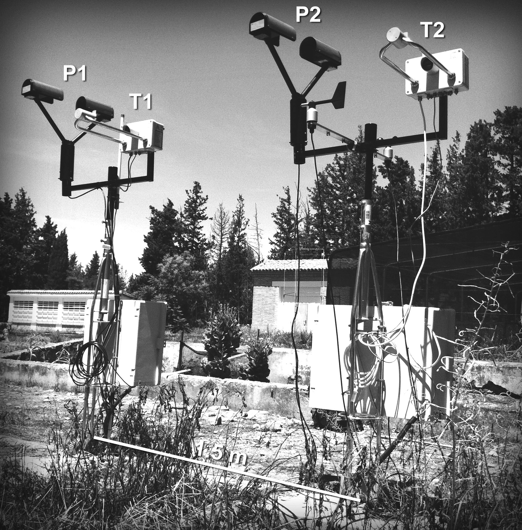
Figure 1Sampling site with four collocated disdrometers: two Parsivel2 (P1 and P2, with serial numbers 304 555 and 304 553); and two Thies (T1 and T2, with serial numbers 0436 and 0655).
Both optical disdrometers, Thies Clima LPM and OTT Parsivel2, are based on the same measurement principle. Their external structure is formed by two heads that connect the sheet of laser light through which falling drops are measured. Drop diameter and fall velocity are determined from the obscuration amplitude and duration in the path of an infrared laser beam, between a light emitting diode and a receiver, within a sampling area of approximately 50 cm2 (Donnadieu et al., 1969; Löffler-Mang and Joss, 2000). Raindrops are assumed spherical for sizes less than 1 mm in diameter, and therefore the size parameter is the equivalent diameter for raindrops below this size. For larger raindrops, a correction for oblateness is made, and the size parameter is interpreted as an equi-volume sphere diameter. The laser signal is processed by a proprietary software, and the size (equi-volume particle diameter) and velocity of each particle is determined. The meteor type (drizzle, rain, hail or snow) is determined based on typical size and velocities, and weather codes (SYNOP and METAR) are generated. A PSVD matrix counting the number Ni,j of particles for a given size (i) and velocity (j) classes is recorded at desired intervals, usually 1 minute. Several integrated variables are also computed and stored at the same intervals. These include the number of particles detected (NP, min−1), the particle density (ND, m−3 mm−1), the rainfall amount (P, mm) and intensity (R, mm h−1), the radar reflectivity (Z, dB mm6 m−3), visibility (m), and kinetic energy (J m−2 mm−1).
This operational principle is subject to a number of potential sources of bias, as reviewed by Frasson et al. (2011). One of these such sources of bias is the uneven power distribution across the laser beam, or variations in this power with time. Also, the geometry of the laser beam limits the estimation of fall velocity in the vertical component, producing biased measurements when the particles fall with a different trajectory or angle due to wind or eddy drag (Salles et al., 1999). Another source of biased measurements is due to the occurrence of coincident particles, which are perceived as just one single drop by the sensor. Similarly, the event of one drop falling at the edge of the laser beam (“margin faller”), therefore being only partially observed, leads to biased measurements. Both sensors mention in their technical data some correction for edge detection (margin fallers) and coincident particles, although there is little information on how these two events are identified and treated. More details of both instruments and the measurement technique, along with the assumptions used to determine the size and velocity of hydrometeors, can be found in Löffler-Mang and Joss (2000), Battaglia et al. (2010), Tapiador et al. (2010, 2017a), Frasson, et al. (2011), Jaffrain and Berne (2011), Tokay et al. (2013, 2014), Raupach and Berne (2015), and in their respective technical manuals.
There are slight hardware variations between the two instruments, as well as differences in how the raw data are treated and converted into the outputted variables. Since these differences may have an impact on the final records, we review the relevant characteristics of each device in the following paragraphs.
2.1.1 Thies Clima Laser Precipitation Monitor
The Laser Precipitation Monitor (LPM) uses a 780 nm laser beam which is 228 mm long, 20 mm wide and 0.75 mm thick on average, resulting in a sampling area of 45.6 cm2. Geometric deviations from this standard are reported by the manufacturer for each particular disdrometer, and for instance the sampling areas of the two devices used in the experiment were 46.65314 and 49.04051 cm2. It records particles starting from 0.16 mm of diameter and precipitation starting from 0.005 mm h−1. The Thies technical documentation indicates that the size and velocity measurements are “checked for plausibility” to prevent issues such as edge events, implying that some particles are filtered out, although the details of this procedure are not specified. From the raw particle data, several bulk variables (“PSVD moments”) are integrated internally by the device's firmware. Drop diameters and velocities are then grouped into 22 and 20 classes ranging between 0.125 and 9 mm and between 0 and 12 m s−1, respectively (see Table 1), and the number of particles recorded at each size and velocity pair bin is stored. The bulk variables computed by the Thies LPM does not include the kinetic energy. In addition, several status flags are provided in the data telegrams informing about voltage oscillations, sensor temperature and an evaluation of the measurement quality.
Table 1Classification or particles according to equi-volume diameter (D) and fall velocity (V) bins by disdrometer type.
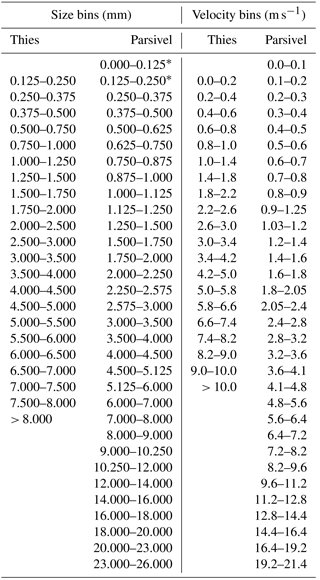
* Left empty by the manufacturer.
2.1.2 OTT Parsivel 2 disdrometer
The Parsivel disdrometers used in this study belong to the second generation manufactured by OTT Hydromet Inc (Parsivel2). The Parsivel2 uses a 780 nm laser beam which is 180 mm long, 30 mm wide and 1 mm thick on average, with no indication about deviations from these values from the manufacturer. The sampling area for the two Parsivel disdrometers was therefore 54 cm2. The Parsivel2 records particles starting from 0.2 mm of diameter, and precipitation starting from 0.001 mm h−1. The measured particles are stored in drop diameter and fall velocity bins in a 32 × 32 matrix with uneven intervals starting at 0 mm diameter up to 26 mm and from 0 up to 22.4 m s−1 (Table 1). The first two size categories, which correspond to sizes of less than 0.25 mm, are left empty by the manufacturer because of the low signal-to-noise ratio. The Parsivel2, similarly to the Thies, also provides a sensor status flag and several control variables in its data telegram.
According to Battaglia et al. (2010), particles up to 1 mm are assumed spherical, and between 1 and 5 mm they are assumed as horizontally oriented oblate spheroids with axial ratio linearly varying from 1 to 0.7, with this ratio being kept constant at 0.7 for larger sizes. The Parsivel technical documentation mentions that the device filters out edge events, although the exact details of this procedure are not given. Battaglia et al. (2010) mention that the newest Parsivel units include two extra photo-diodes at the edge of the laser beam to detect and remove the edge events, but the manufacturer provides no information about this. Independently to filtering out edge events, Löffler-Mang and Joss (2000) indicate that a correction of the effective sampling area is used depending on the particle size. Some sources (Tokay et al., 2013) also refer to a correction to the fall velocity is applied to drop sizes between 1 and 5 mm, although once again there is no more information on this correction. Parsivel2 disdrometers external structure differs from the Thies LPM in incorporating a splash protection shield above the laser heads, which aims at minimizing the effect of splashed drops that interfere with a high velocity with the laser beam and result in biased measurements.
2.2 Processing disdrometer data
One-minute disdrometer data telegrams were stored in an industrial miniature PC (Matrix 504 Artila Inc). The PC included custom software to collect, pre-process and send data telegrams to a central server. Time synchronization was performed once per day using the Network Time Protocol (NTP), allowing bias correction of the internal disdrometer clocks that have a tendency to drift. Direct reading of the data telegrams generated by the disdrometers resulted in 1 min time series of the variables of interest for this study: PSVD matrices (Ni,j), bulk variables (P, R, NP, ND, Z, E), SYNOP codes, and status and error flags. An exception was Thies disdrometers, which do not compute the kinetic energy, E. Parsivel, on the other hand, gives the kinetic energy expressed in Joules, so it was divided by the sampling area and the rainfall amount to obtain E.
In addition to the bulk variables computed by the internal software of the devices, the bulk variables were computed again from the PSVD matrices, using the following expressions:
where ρ is the density of water (1000 kg m−3), Di is the mean diameter of class i, Vj is the mean velocity of velocity class j, and Δt is the sampling frequency (s). The effective sampling area, Ai (m−2) depends on the particle size, since in order to be correctly sensed the particles need to be inside the light beam in its entirety, so
where A is the sampling area of the disdrometer and w is the width of the laser beam. As it can be seen, the effective sampling area gets reduced as the drop size increases, and the magnitude of the correction applied is inversely proportional to w.
This allowed, on the one hand, for obtaining E for Thies disdrometers, but also permitted to apply a number of corrections that simplified the comparison between the two types of disdrometer. Thus, we ignored the particle counts in the first size bin of Thies disdrometers and the counts in the size bins larger than 8 mm, so the two disdrometer types were measuring the same range of drop sizes (0.25 to 8 mm). We also applied a filter to remove highly unlikely drop size and velocity combinations, as done in many studies (e.g. Tokay et al., 2001, 2013; Jaffrain and Berne, 2011; Raupach et al., 2015). In order to do that, each size and velocity bin was compared with the terminal fall velocity model of Beard (1976), and the bins for which a difference larger than 50 % existed with the theoretical model were excluded.
In order to compare PSVD data between disdrometer types, the 10th, 50th and 90th percentiles of the particle size (D10, D50, D90) and velocity (V10, V50, V90) were computed (Table 2). One problem that arises when percentiles are computed from binned data is that the resulting percentiles may be biased depending on the binning structure of the data. If all the particles recorded in one bin are assigned the mean value of the bin (the easiest option), different bin configurations will lead to different computed percentiles, even if the raw data before binning were identical. When data from different binning structures are compared, as it is the case here between Thies and Parsivel disdrometers, an interpolation scheme needs to be used for distributing the range of values within each bin across all the particles corresponding to that bin. Here we used a random distribution over the range of values in the bin following a linear probability distribution constructed by fitting a line between two points determined as the average of the number of particles in the bin and the corresponding values on the neighbouring bins. Given the high number of particles detected, the random component of this scheme has a negligible effect on the results. Once all the number of particles by minute were assigned particle size and velocity values, the percentiles were calculated, allowing for a comparison between disdrometers.
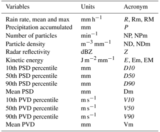
In addition to 1 min data, the mean (m) and maximum (M) values of some of these variables (Rm, RM, KEm, KEM, Em, EM, NPm) were computed for each rainfall event. A summary of the variables analysed is provided in Table 2.
Table 2Disdrometer evaluated variables. M and m stand for maximum and mean, respectively.
All data processing, including reading the raw telegrams, computing the
integrated variables (erosivity for Thies LPM and size and velocity
percentiles) and plotting, was performed using a custom package for the R
environment, disdRo (Beguería and Latorre, 2018).
2.3 Comparison of disdrometer measurements
Prior to any analysis, minute observations with low quality or bad sensor status flags were removed from the comparison dataset. Minutes with missing data, precipitation below 0.1 mm h−1 or less than 10 particles detected in any of the four disdrometers were also removed. This way, only minutes with good quality data in the four devices were considered in the analysis. The comparison was made primarily on the bulk variables computed from the PSVD matrix stored in the 1 min telegrams outputted by the four disdrometers, by applying Eqs. (1) to (6). We also compared the bulk variables calculated by the internal firmware of the devices, in order to check the impact of the effective sampling area correction and the removal of unlikely size–velocity bins.
Kernel density and violin plots, i.e. non-parametric graphical estimations of the probability density functions of the variables, were used as a preliminary analysis tool. A formal comparison between the two disdrometer types was performed using a Gamma generalized linear mixed model (Gamma GLMM), with the bulk variables listed in Table 2 as response variables. Mixed models allow incorporating both fixed effects and random effects in the regression analysis (Pinheiro and Bates, 2000). The fixed effects describe the values of the response variable in terms of explanatory variables that are considered to be non-random, whereas random effects are treated as arising from random causes, such as those associated with individual experimental units sampled from the population. Hence, mixed models are particularly suited to experimental settings where measurements are made on groups of related, and possibly nested, experimental units. If the grouping factor was ignored when modelling grouped data, the random (group) effects would be incorporated into the error term, leading to an inflated estimate of within-group variability. This allowed us to assess differences in the response variables as a function of the disdrometer type (fixed factor), while controlling for possible differences due to the location of the two masts (random factor). Since the explanatory variable is a dichotomic variable (the disdrometer type), this configuration is equivalent to a random effects analysis of variance (ANOVA). A Gamma distribution was used to model the response variables, since this distribution is best suited to positive data with variance increasing with the mean, as it is the case for the disdrometer variables analysed here. This model configuration can be described as
where yi is the ith observation of the response variable Y; ν is a shape parameter; θi is a scale parameter, which can be expressed in terms of ν and a mean value corresponding to the ith observation μi; μ is a global mean; βt(i) is a parameter accounting for the effect of the disdrometer type corresponding to observation i, t(i); and αm(i) is a parameter accounting for the location (mast) corresponding to observation i, m(i). In our case, we counted with four disdrometers grouped into disdrometer types (Thies and Parsivel, respectively), and located in masts, and we set . For the link function g(μi) we used an identity link, g(μi)=μi, except for R, Z, E and NP for which a log link, g(μi)=log μi, was used.
The model in Eq. (2) was fitted by generalized least squares (GLS),
using the function lme from the R library lme4 (Pinheiro
and Bates, 2000). A random sample of N=1000 records, corresponding to
250 min, was used in the analysis, in order to avoid size effects negatively
affecting the statistical significance tests (Type I error inflation; see,
e.g. Lin et al., 2013).
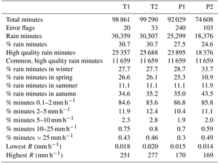
A summary report on the data acquired by the four disdrometers is reported in Table 3. Almost 100 000 min of data were obtained from each device. Missing values due to technical issues (power supply failures and device hangouts, data communication problems) were found in all disdrometers, although they were more prevalent on one of the Parsivels (P2), resulting in a significantly lower number of records by this device. The number of errors, as reported by the status flags of the devices, was low, albeit larger in Parsivel than in Thies devices. Some records were discarded due to quality issues, either based on the quality flat reported by Thies (only data with quality flags above 90 % were accepted) or on inconsistent data in the telegram (saturation of the PSVD bins or excessively large-intensity values) in the Parsivels. Since Parsivel does not report the data quality, no quality threshold could be used. Around 31 % of the minutes recorded rain hydrometeors in both Thies, while this percentage was lower for Parsivel (27.5 % in P1; the value of P2 was even lower, but can not be considered since this device recorded a significantly reduced number of minutes due to technical issues). The larger amount of minutes with rainfall in Thies disdrometers can be attributed to their higher sensitivity, since they are able to record smaller raindrops (more on this later).
All types of precipitation events occurring in the sampling site were represented, with the majority of observations corresponding with autumn rains, as corresponds to the climatology of the area. Rain rates varied between 0.014 and 277 mm h−1. The minimum precipitation rates were between 0.014 and 0.020 mm h−1, with no differences between devices. The absolute maximum precipitation rates measured during the experiment depended on the disdrometer type, with Thies being the ones recording the highest values.
As mentioned in Sect. 2.1, only the common minutes were selected from the complete dataset, defined as those having high quality data and detection of rainfall particles in each of the four disdrometers. This led to a total of 46 636 records, corresponding to 11 659 min belonging to 157 rainfall episodes.
Table 3Disdrometer data summary. Number of minutes recorded, errors, minutes with rain (SYNOP codes 61, 63 and 65), and high quality minutes; percentage of records in each season, and by rain intensity ranges; and maximum rain intensity.
When considering only the records for which data of the four disdrometers existed, the total accumulated precipitation as measured by the disdrometers internal software was 244.9 mm (T1), 254.5 mm (T2), 220.4 mm (P1) and 228.1 mm (P2). These values were slightly different to those calculated from the PSVD data, which were slightly lower at 240.1 mm (T1), 253.0 mm (T2), 218.6 mm (P1) and 222.0 mm (P2). A graphical comparison of the cumulative time series for the computed and internal precipitation is provided in Fig. 2. Some discrepancies in total precipitation were therefore found between the devices, with the two Thies LPM devices recording more precipitation than the Parsivel ones. Between locations, mast 2 tended to record larger precipitation in both devices, although the magnitude of this difference was much lower than the difference between disdrometer types.
Differences were also found with respect to cumulative kinetic energy, for which larger values were also found for Thies (2100 and 2101 J m−2 mm−1) than for Parsivel (1749 and 1829 J m−2 mm−1). This corresponds to values obtained from the PSVD data, since Thies disdrometers do not calculate the kinetic energy internally. Unlike with P, for E there were important differences between the values measured by the Parsivel2 disdrometers (2100 and 2181) and those calculated from the PSVD, reported above.
This result suggests that differences between devices could be due, to a certain extent at least, to Thies LPM devices being more sensitive in the lower range of the PSVD spectrum, although this hypothesis requires further analysis, as done in the following sections.
3.1 Example events
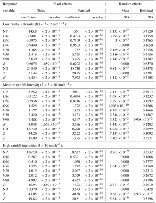
Two events, representative of low and high precipitation intensity rates, were selected to illustrate the differences between disdrometer outputs. Time series of some bulk variables are shown in Figs. 3 and 4. In both events, Thies devices consistently reported higher rainfall intensity and cumulative precipitation. This is related to a larger number of rain particles detected, as shown by the number density (which factors out the different rain intensities). There were also differences in the median particle size, which was much larger in the Parsivel devices. Interestingly, it seems that these differences (larger number of drops in Thies, but larger mean size in Parsivel) somehow cancelled out for radar reflectivity and kinetic energy, which depend both on the number of drops, their size, and velocity.
These differences were most evident in the high-intensity event, and were also higher if no corrections for unlikely drops and effective sampling area were performed (Appendix, Figs. A1 and A2).
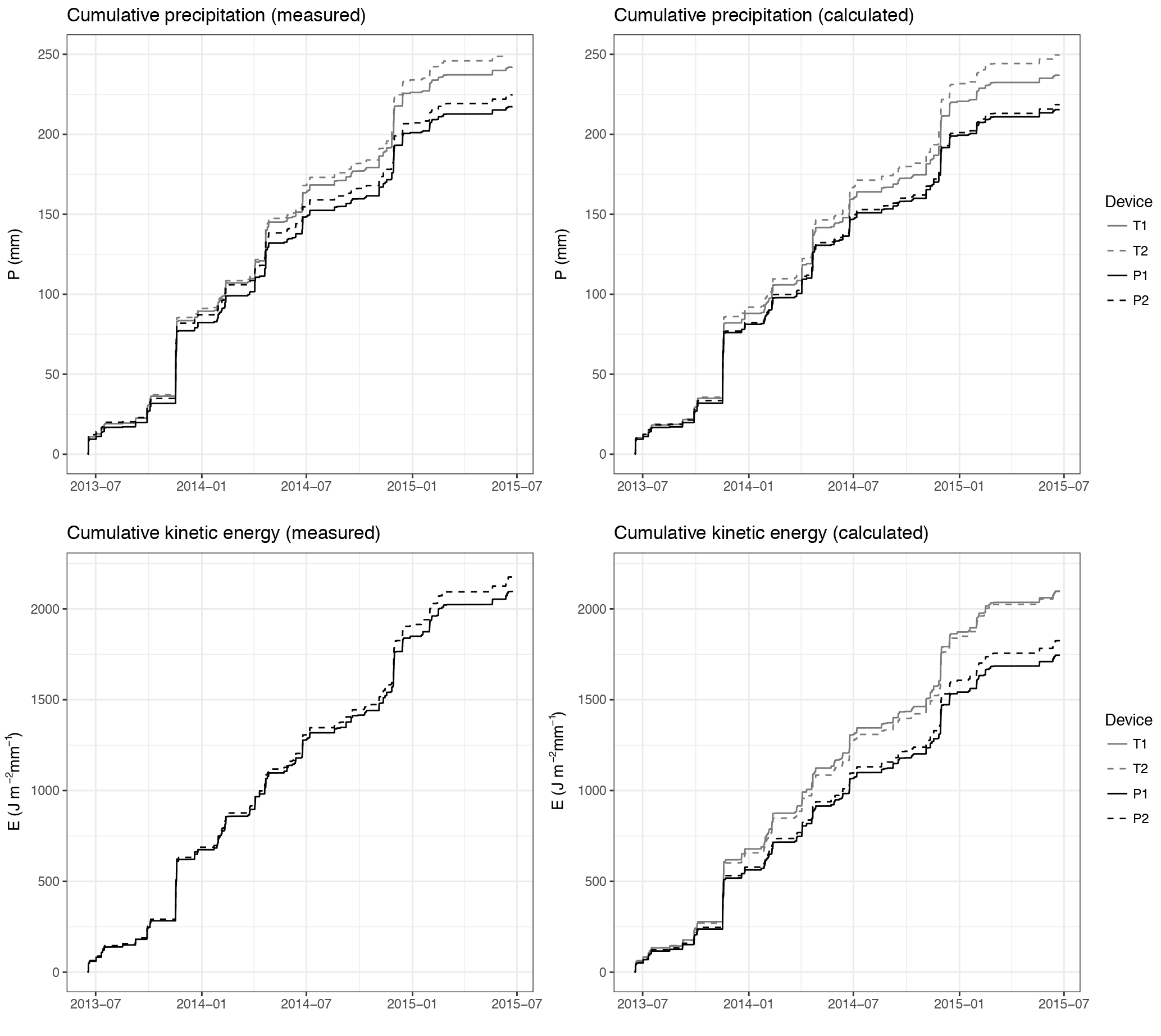
Figure 2Accumulated precipitation (R, mm) and kinetic energy (E, J m−2 mm−1) during the 2-year experiment (only the minutes with data on the four disdrometers are used).
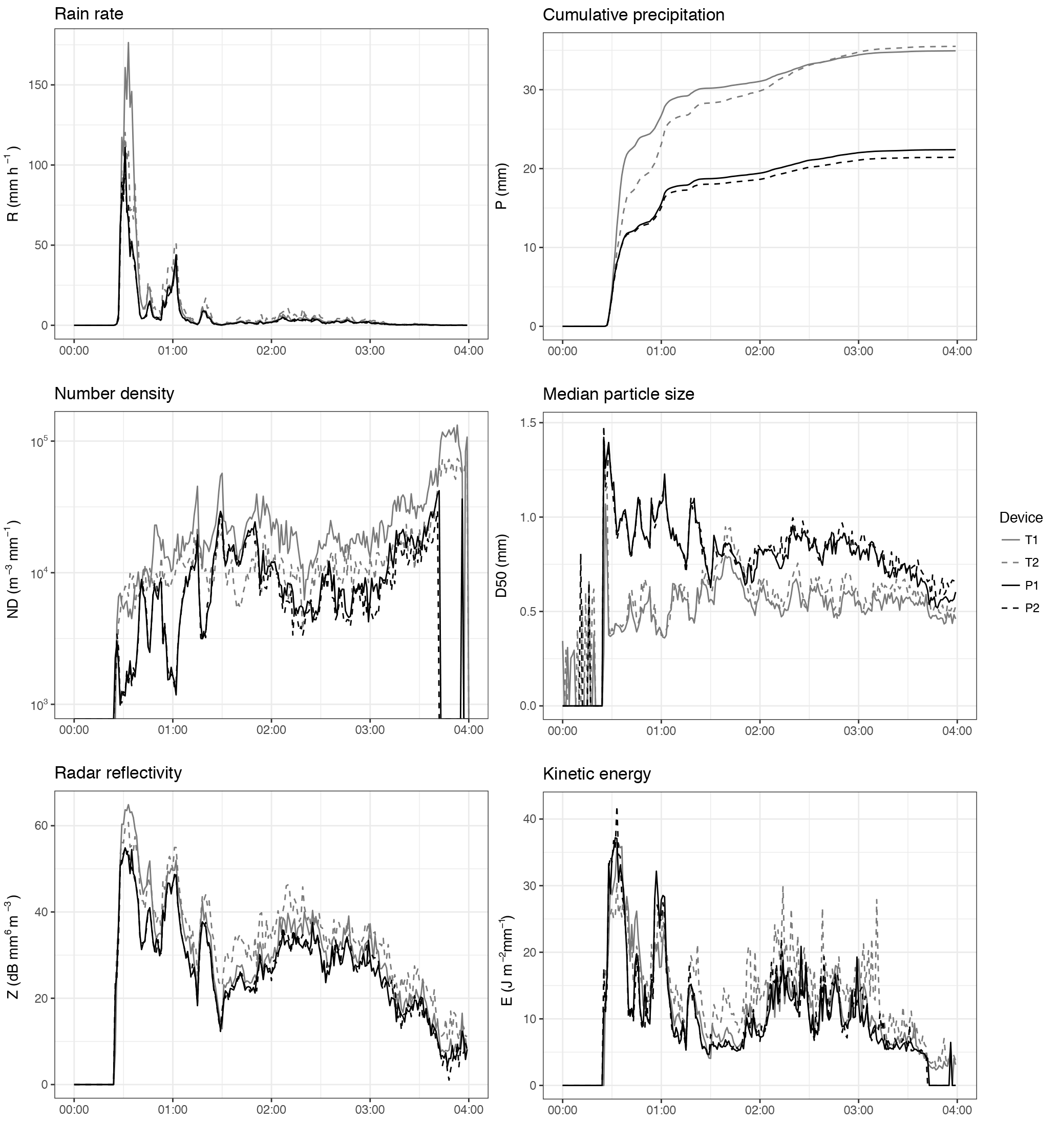
Figure 3Time series of disdrometer bulk variables during a high-intensity event (E365, 25 November 2014).
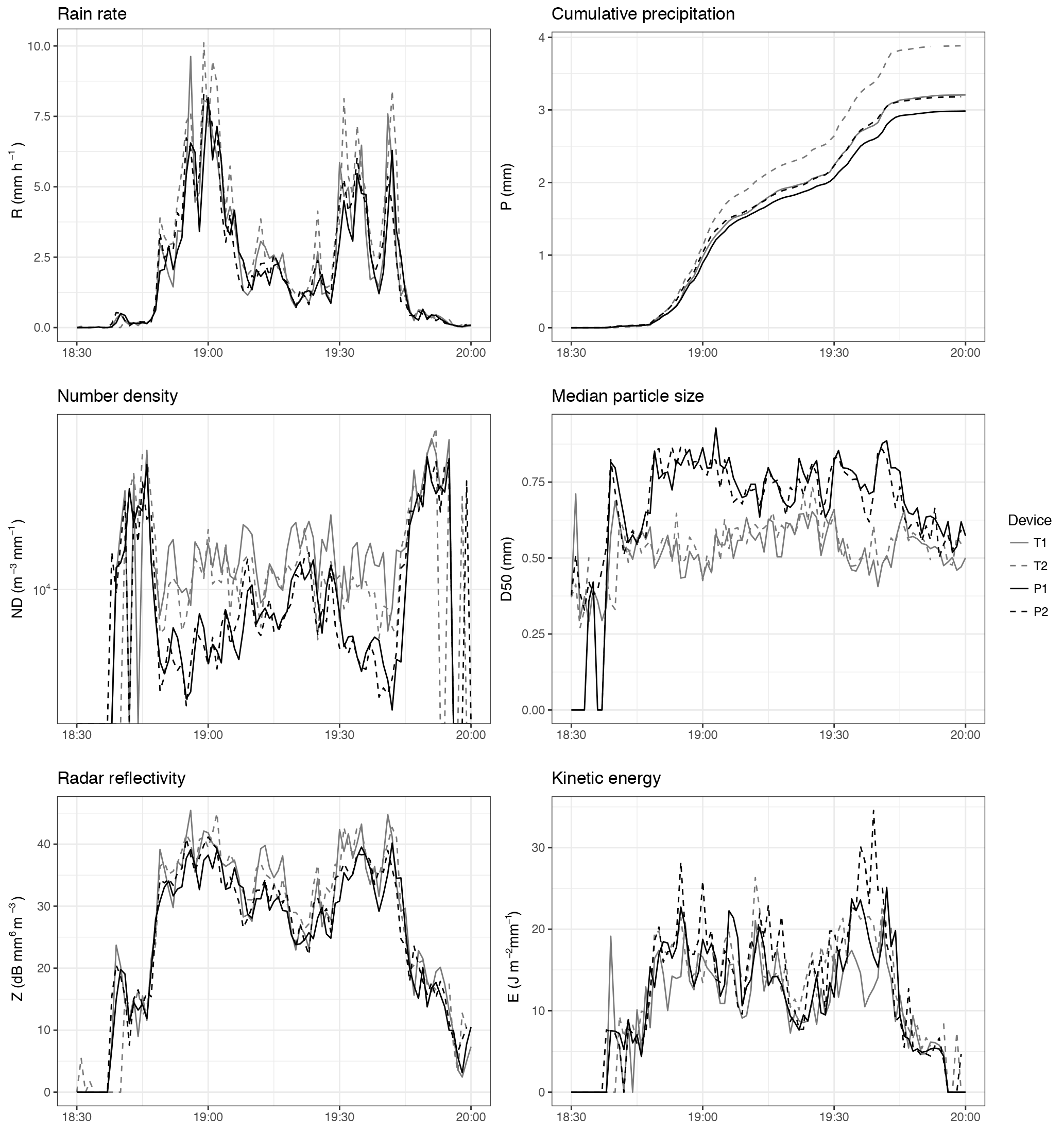
Figure 4Time series of disdrometer bulk variables during a low-intensity event (E455, 23 February 2015).
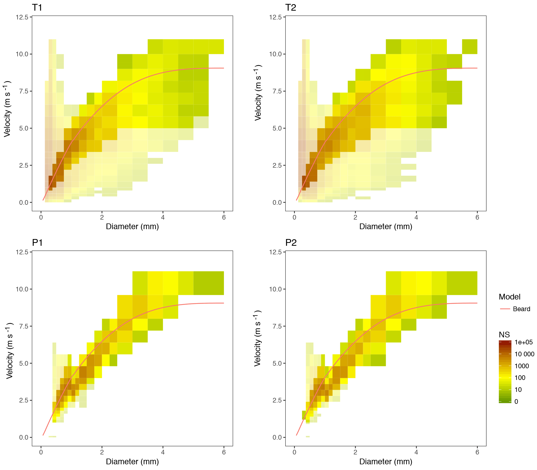
Figure 5Particle size and velocity density (PSVD) plots of a high-intensity event (E365, 25 November 2014). The colour scale indicates the number of particles for each size and velocity class (NP). Deviations larger than 50 % from the theoretical terminal velocity model (Beard, 1976; red line) are indicated with a 50 % transparency.

Figure 6Particle size and velocity density (PSVD) plots of a low-intensity event (E455, 23 February 2015). Legend as in Fig. 5.
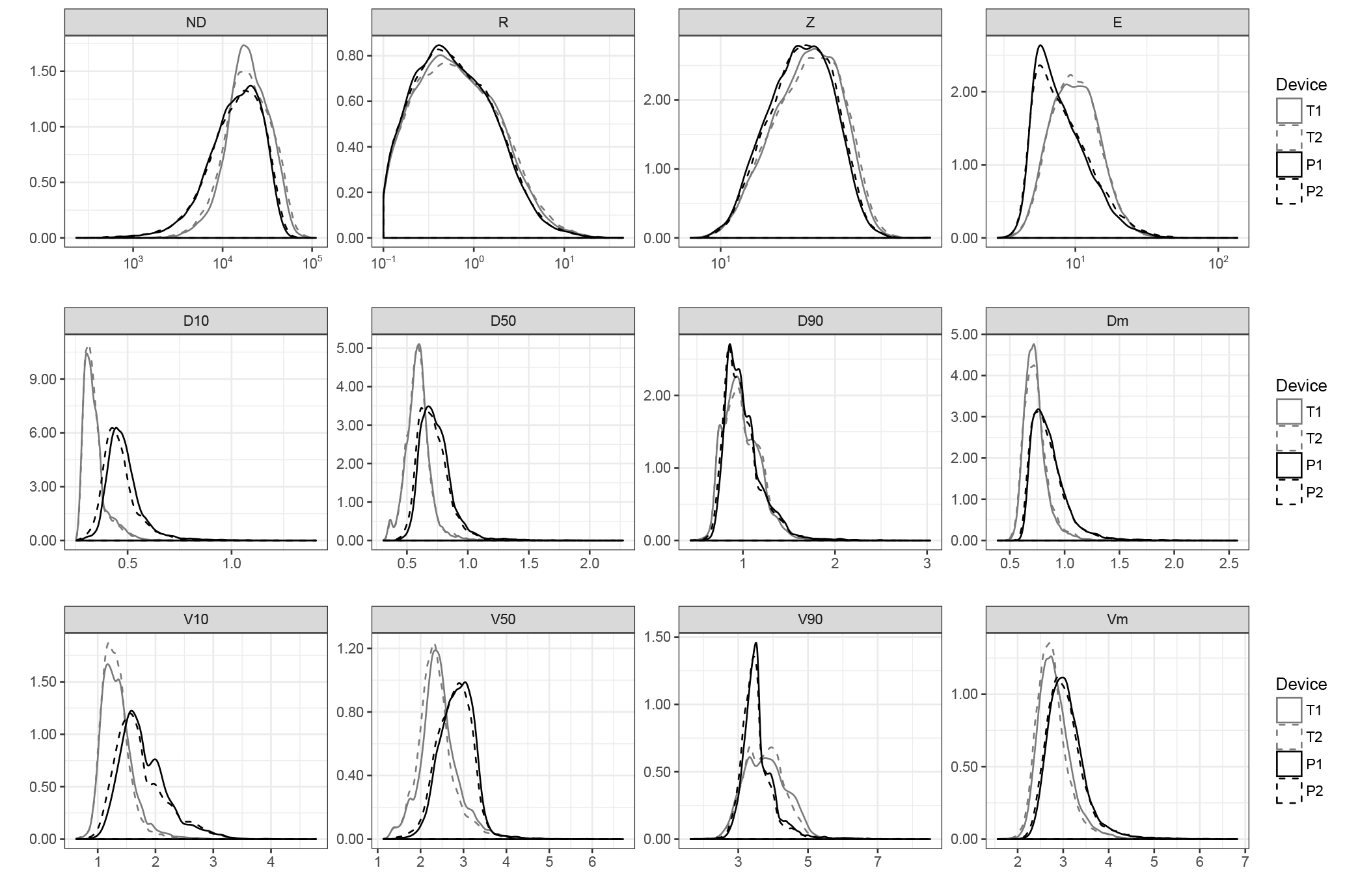
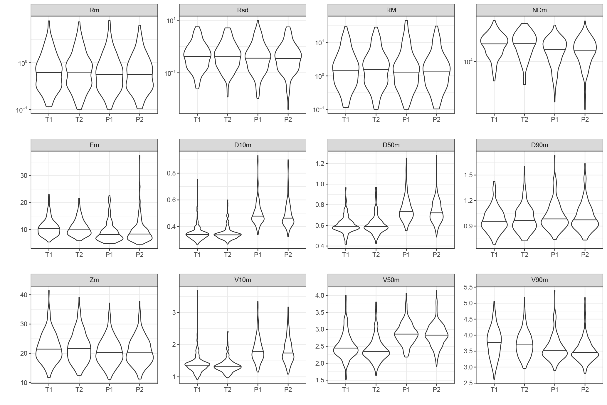
Figure 8Violin plots for event means and maxima. Refer to Table 2 for a list of acronyms of the variables.
The PSVD plots (Figs. 5 and 6), depicting the number of drops detected for each combination of drop size and velocity classes during the event by each disdrometer, help explain the differences found. A first and evident difference is that Thies disdrometers had a much wider distribution of the PSVD spectra than Parsivel ones. The terminal velocity of raindrops as a function of their size according to Beard (1976), also depicted in the figure, was used to filter out unlikely combinations of size and velocity. Combinations which differ by more than 50 % with the theoretical fall velocity are represented in the figure with a 50 % transparency. Although a majority of particles were found to lie in a region close to the theoretical line, Thies devices had a much larger number of particles far from the theoretical model, both in the high- and low-intensity events. Particularly, a large number of very small particles at much higher velocities than expected was very prominent, as were the drops with a large diameter but a fairly low velocity. Typically, the first case (small, fast raindrops) are attributed to edge events (partial recognition or larger drops falling in the edge of the laser beam), or splashed particles, while the second case is interpreted as double detections (two or more simultaneous drops). Both effects tend to increase with the precipitation intensity, as the anomalous events become more frequent.
The frequency of anomalous raindrops was much lower in the Parsivel output, for which the vast majority of cases fell within the theoretical model limits. This can be attributed to a number of facts. From pure geometrical considerations, a larger prevalence of edge events can be expected from Thies, since its laser beam has a reduced width (20 mm) with respect to Parsivel (30 mm), so the proportion of edge events with respect to the number of particles detected is higher. Other reasons such as a larger proneness to splashing or differences in the internal processing of the data (that, as stated by the manufacturers, includes some filtering of anomalous data), may also help explain this differences.
Finally, and interestingly, an underestimation of drop velocities with respect to the theoretical model could be found in Parsivel devices, most notably in the high-intensity event and for particles larger than 1 mm.
A formal analysis of these differences, considering the whole dataset, is presented in the following section.
3.2 Integrated variables – minute timescale
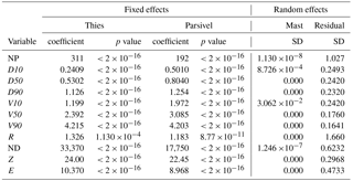
When the whole dataset was analysed, differences between disdrometers were also evident, as shown by the exploratory kernel density plots (Fig. 7). This was further confirmed by the Gamma GLMM analysis (Table 4). The coefficients reported in the table for the fixed effects correspond to βT and βP when μ is set to zero in Eq. (2), and can be interpreted as the mean values of the response variables for each disdrometer type, when other factors (the mast in this case) are accounted for. The table includes also the p values corresponding to these coefficients, as well as the residual and mast standard deviation (σ and σm(i), respectively).
The analysis yielded significant differences between disdrometer types for all the response variables analysed, while the random effect (the mast) had a negligible effect as shown by its small variance with respect to the random error (residual). There were substantial differences in the number of particles detected, NP, and in the PSVD percentiles. Thus, Thies disdrometers had a lower coefficient for NP (230 vs. 194), indicating a tendency to detect a higher number of particles (an increase of circa 20 %). Thies also had much lower coefficients for D10 and D50 (0.59 vs. 0.74 for the median drop size, i.e. a decrease of circa 20 %), as well as for V10 and V50 (2.4 vs. 2.9, i.e. an 18 % difference). The magnitude of the difference was lower for the highest percentiles (D90 and V90), where Thies even had a higher coefficient for velocity, indicating a larger spread of velocities compared to Parsivel.
These differences in the number of particles and in the PSVD were translated to the bulk variables, which also showed significant differences in all cases. The magnitude of the effect, i.e. the mean differences between the two disdrometer types, were high for the particle density (21 600 vs. 15 920, a 36 % increment) and kinetic energy (11.09 vs. 9.66, i.e. a 15 % difference), while they were smaller (albeit significant) for R and Z (12 and 7 % difference, respectively).
The differences found in the PSVD percentiles allow for a better understanding of the differences in the integrated variables, since the particle size and velocity have contrasting effects on R, ND, Z and E. In general, a higher number of particles implies increasing values of all these variables, which favours Thies devices since it tended to detect a higher number of particles. The particle size, on the other hand, has a similar effect of increasing all the variables for which it is relevant (R, Z and E). Since the particle size was in general higher in Parsivel devices, this effect partially cancels out the effect of the increasing number of particles. Particle velocity, which was in general higher in Parsivel (except for the largest drops), has a positive effect in E, but a negative effect on Z, which further explains the differences found. The particle density (ND), finally, is not affected by the drop size and is negatively affected by fall velocity, and that the reason why this variable showed the highest difference between both disdrometers.
3.3 Integrated variables – event scale
Although one of the benefits of the optical disdrometers is their ability to provide large amounts of information at very fine temporal scales (as 1 min data analysed here), very frequently these data are aggregated over larger time periods or rainfall events for practical issues. For instance, it is typical for the computation of kinetic energy totals for rainfall events; for instance, for soil erosion applications. When considering the same variables at the event level, looking at the mean and maximum values over the event, similar results were found (Fig. 8 and Table 5).
Again, significant fixed effects were found for all response variables, while the random effect was marginal in all cases. The average number of particles during the events was much larger for Thies, and the median drop size and velocity was lower. There were also differences, although of smaller size, in the rest of integrated variables.
3.4 Effect of PSVD data correction
The effect that the data correction scheme may have on the integrated variables merits some analysis, since it modifies the PSVD distribution. Here we applied a filter that consisted of eliminating the unlikely drops, which was aimed at eliminating edge events and double detections, while a correction for the sensing area as a function of the drop size was applied to compensate for the loss of mass. The results shown in the previous sections were all based on the corrected data, but in order to determine the effect of this correction on the computed variables, the analysis was replicated without applying the filtering and the correction.
The results are shown in the Appendix, in Table A1 and Fig. 7. A comparison with the results shown in the previous section reveals the same general pattern, but with stronger effects. For instance, the coefficient for the number of particles NP was 62 % higher in Thies than in Parsivel. Interestingly, the effect of the correction on the particle size percentiles had a different sign in Thies, for which D50 increased from 0.53 (without correction) to 0.60 (with correction), while in Parsivel it decreased from 0.80 to 0.74. For the median particle velocity (V50), the coefficient remained very similar before and after correction for Thies, while for Parsivel it increased from 2.88 to 3.09 (7 %). The relative magnitude of the differences between Thies and Parsivel disdrometers was 88 % for ND, 12 % for R, 15 % for E and 7 % for Z, i.e. much higher than after filtering and correction for ND but similar for the other three variables.
3.5 Effect of rainfall intensity
Data were divided by intensity ranges in order to test if the effect of the disdrometer type changed with different rain intensities. As the rainfall intensity increases, it is expected to find more and bigger drops, which may in turn modify the differences found between disdrometer types. Data were thus divided into three intensity groups: low intensity (from 0.1 up to 2 mm h−1), medium intensity (from 2 up to 10 mm h−1) and high intensity (more than 10 mm h−1). Model coefficients for the three intensity ranges are given in Table 6, and kernel density plots can be found in the Appendix (Figs. A4, A5 and A6).
Table 4Gamma generalized linear mixed-effects model coefficients for 1 min records (random sample size of N=1000). Refer to Table 2 for a list of acronyms of response variables.
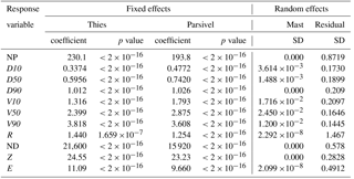
Table 5Gamma generalized linear mixed-effects models coefficients for event totals (sample size N=624). Refer to Table 2 for a list of variable acronyms.
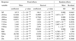
Table 6Gamma generalized linear mixed-effects model coefficients for minutes with varying rainfall intensities.
The same effects described above were found at different rainfall intensities. The magnitude of the effects, however, tended to increase with the intensity. Thus, the relative difference between the coefficients of NP ranged between 7 % (146 vs. 136) for low rainfall intensity, 27 % for medium intensity and 65 % for high intensity, while the median particle size ranged between 16, 28 and 200 %. Equally large were the relative differences between the coefficients of ND, which varied between 33, 67 and up to 292 %, while for the remaining variables the increase in the effect with the rainfall intensity was less pronounced.
Optical disdrometers are commercially affordable sensors able to provide a thorough description of precipitation, and they are being increasingly used by national weather services as present weather sensors and even rain gauges requiring low maintenance. Besides their use in operational networks, optical disdrometers provide information on precipitation drop spectra that has applications in different fields, and they are being increasingly used in research.
Thies Clima LPM and OTT Parsivel2 are among the most common, state of the art, optical disdrometers. Despite being based on the same functioning principle and having similar characteristics in terms of sensitivity and range of particle detection, there are substantial differences between them that may differently affect their records. We have stressed the differences in the higher and (more important) lower particle size detection ranges of the two devices, with Thies having a lower detection threshold that may induce bias in the records of the two disdrometer types. Filtering the PSVD matrix to a common detection range, as done here, allows for a fair comparison between the outputs of the disdrometers, and should be recommended for any study that aims at presenting general results. However, as we have seen here, despite applying the same detection thresholds to the data outputted by the two disdrometers, significant differences were found both at the level of PSVD spectra (particle size and velocity percentiles) and on the bulk variables (PSVD moments).
There are a number of factors that may help explain the differences found. Geometrical differences between the laser beams are highly relevant, since they greatly influence the probability of bias-inducing effects such as edge events (margin fallers) and double detections. A larger sampling area, for instance, implies a higher chance of double detections. In this respect, the larger sampling area of Parsivel (54 cm2) over Thies devices (45.6 cm2 on average) implies that Parsivel disdrometer should be more affected by double detections. Double detections, i.e. time-overlapping drops, may be sensed just as one single drop (hence causing a loss of mass which may translate to a reduced precipitation record); or as a much larger drop at an unusually low velocity. Since these unusual particles are often discarded from the PSVD matrix, this may result in another source of mass loss, which may or may not be partially solved by the sampling area correction (more on this later). Although this would require further research, for instance with the help of numerical simulations as in the work by Raasch and Umhauer (1984), we suspect that the tendency towards a lower number of particles detected and lower precipitation amounts found on Parsivel devices may have a relationship with this effect.
But geometrical effects are not restricted to this. Since the effective sampling area of optical disdrometers depends on the particle size, not only the total area but also the width of the laser beam plays an important role as a source of bias. In particular, the proportion of edge events (i.e. particles that are sensed only partially due to falling at the edge of the laser beam) over the total number of particle detections of the same diameter class is inversely proportional to the width of the beam. The smaller width of the laser beam on Thies (20 mm) over Parsivel (30 mm) plays against the former, which should be more prone to affects by edge events. This becomes more relevant for the higher particle bins. For 5 mm particles, for instance, the effective width gets reduced to 15 mm for Thies, i.e. a reduction of 25 %, while for Parsivel this reduction amounts to 16.6 %. Edge events result in partially sensed particles, implying a mass loss and an overestimation of fall velocity. The high prevalence of over-accelerated, small particles in the PSVD spectra of Thies disdrometers may be related to this effect; although again, further analysis is required in order to confirm this hypothesis. In this respect, the Thies manufacturer checks and reports the deviations due to fabrication tolerances from the theoretical geometrical properties of the laser beam on each device, whereas this information is not given for Parsivel.
In order to overcome these problems, we applied a correction scheme which is similar to the ones found in other studies (e.g. Löffler-Mang and Joss, 2000; Battaglia et al., 2010; Raupach and Berne, 2015). The scheme consists of two parts: the first implies removing highly unlikely particle counts, i.e. those with velocities that are far from the theoretical fall velocity corresponding to their size. These unlikely particles are most possibly caused by edge events and double detections, so they are removed from the PSVD data. This causes a loss of mass, and this loss of mass is uneven since it increases with the particle size (due to the geometric effect explained above), so the second part of the scheme consists of correcting the effective sampling area used in calculating the bulk variable from the PSVD (Eq. 1). The correction, however, is not guaranteed to restore all the mass loss, and careful calibration is required in order to match the filtering of unlikely particles (which depends on the threshold used for particle removal) with the effective area correction. Here we used a threshold corresponding to a difference higher than 50 % with respect to the theoretical fall velocity matched to a factor of 0.5 of the drop diameter for the area correction, but other combinations are possible. Again, numerical simulation should help in determining the best correction parameters, which in turn should consider the different beam geometries.
Our results showed differences between the two disdrometer types, which were not totally removed by the correction scheme (although they were partially diminished with respect to the un-corrected records). Differences in the internal treatment of the data by the two devices, which is not public, may also help explain this differences. Both manufacturers indicate that some treatment of unlikely detections is performed internally, but very little detail is given. From the examination of the raw PSVD matrices, it seems that the correction applied by Thies, if any, is very subtle, while the output of Parsivel seems to be much more affected by corrections. The technical literature, also gives more detail in the case of the Parsivel, for which at least a correction for the effective sampling area is reported (Löffler-Mang and Joss, 2000). The exact nature of these corrections, however, is not known, or even if they are applied to the integrated variables only or also to the PSVD data. This uncertainty makes it difficult to implement an effective correction scheme that makes the outputs of the two disdrometer comparable.
The external structure of the devices also plays an important role and may lead to incorrect drop detections due to turbulence (see, for instance, Constantinescu et al., 2007, for a review of turbulence-induced errors in pluviometers) and splashing (particles intercepted by the enclosure of the devices which break and splash away in smaller but accelerated drops, see Kathiravelu et al., 2016). It seems that the Thies disdrometer is more prone to having splashed drops interfering with the laser beam, since it contains larger flat surfaces susceptible to splashing particles in the direction of the sensor. The Parsivel units, on the other hand, do not have flat surfaces and include a splash protection shield that seems to effectively reduce the risk of splashing. These morphological differences may also affect differently in case of wind, since the turbulence generated may be very different on both devices, and may also be a cause of systematic bias between the two disdrometers. A future study using high speed video and a wind-tunnel setup could help examine the occurrence and magnitude of these effects, which are poorly quantified up to now.
Finally, we also detected a tendency towards underestimating the velocity of falling particles in the case of the Parsivel units, especially in the range between 1 and 3 mm. This has been shown previously and according to Tokay et al. (2014) this issue is known to the Parsivel manufacturer who mentioned that it is in the process of being fixed. However, at least for the units tested, units still suffered from the same problem. Underestimation of the fall velocity may have a substantial influence on the bulk variables computed from the PSVD data, since the velocity intervenes in several of the equations. Systematic underestimation of fall velocity has an effect of increasing ND and Z, while it decreases E.
Differences in the number of particles detected, and biases in the estimation of particle size and velocity, result in complex biases in the integrated variables. This is due to the different effects that these factors have on their computation, since, depending on the case, there are linear or inverse relationships involved. This stressed the relevance of not only an unbiased estimation of the PSVD by the disdrometers but also of any filtering and correction scheme applied to the PSVD data during post-processing.
The two types of disdrometer analysed showed different PSVD spectra for the same rainfall events, while the differences between the two devices of the same type were much smaller and compatible with random differences. In particular, Thies devices recorded a much larger number of drops than Parsivel2, but also a much larger spread of the PSVD spectra, with a significant amount of drops with unexpected combinations of size and velocity, most notably small drops with excessively high velocities, compatible with edge events (“margin fallers”). Parsivel2 devices, on the contrary, recorded less drops and a PSVD spectra which was much closer to the theoretical model. They also had a tendency towards underestimating drop velocity with respect to both Thies and a theoretical fall model.
Differences in the PSVD spectra resulted in significant discrepancies between both disdrometers in all bulk precipitation parameters such as rain intensity and amount, particle density, radar reflectivity or kinetic energy. These differences were found when these variables were computed by the internal firmware of the devices, but also when they were computed by us from the PSVD data. When the PSVD data were filtered by considering only particles with diameters between 0.25 and 8 mm and by removing unlikely drop size and velocity pairs, and a correction for the effective sampling area was used, the magnitude of the differences was reduced although the tendency remained. In all cases, the differences increased with precipitation intensity, as did the variance between devices of the same type, in agreement with the expectation and with previous studies.
The differences found may be explained by hardware or software differences. Geometrical differences with the laser beams of the two devices translate to a different prevalence of bias-inducing effects such as edge events and double detections, while differences in the external design may also have a large influence on the drop splash. The manufacturers of both disdrometers indicate that corrections have been implemented to prevent or reduce the magnitude of these effects, but the exact procedures are not documented. Different solutions can be adopted to limit undesired effects, both at the hardware and the software level, and inspection of the resulting PSVD spectra during the same rainfall events suggests that the level of correction is higher in the case of Parsivel than in the case of Thies. Wether these differences are (total or partially) due to hardware and design differences, or they are caused by hardware or software filtering and correction of the PSVD data, is still a question with no clear answer. Since some crucial aspects of the internal functioning of both devices are hidden from the final user, it is very difficult to design a data treatment process that would enable making the records of Thies and Parsivel disdrometers compatible and comparable across studies.
The complete dataset and code used to produce the figures and analysis in the current research article can be found in Beguería (2018). The R library disdRo (Beguería and Latorre, 2018) is required for reading and handling meteorological particle size and velocity distribution (PSVD) data from Thies LPM and OTT Parsivel optical disdrometers.
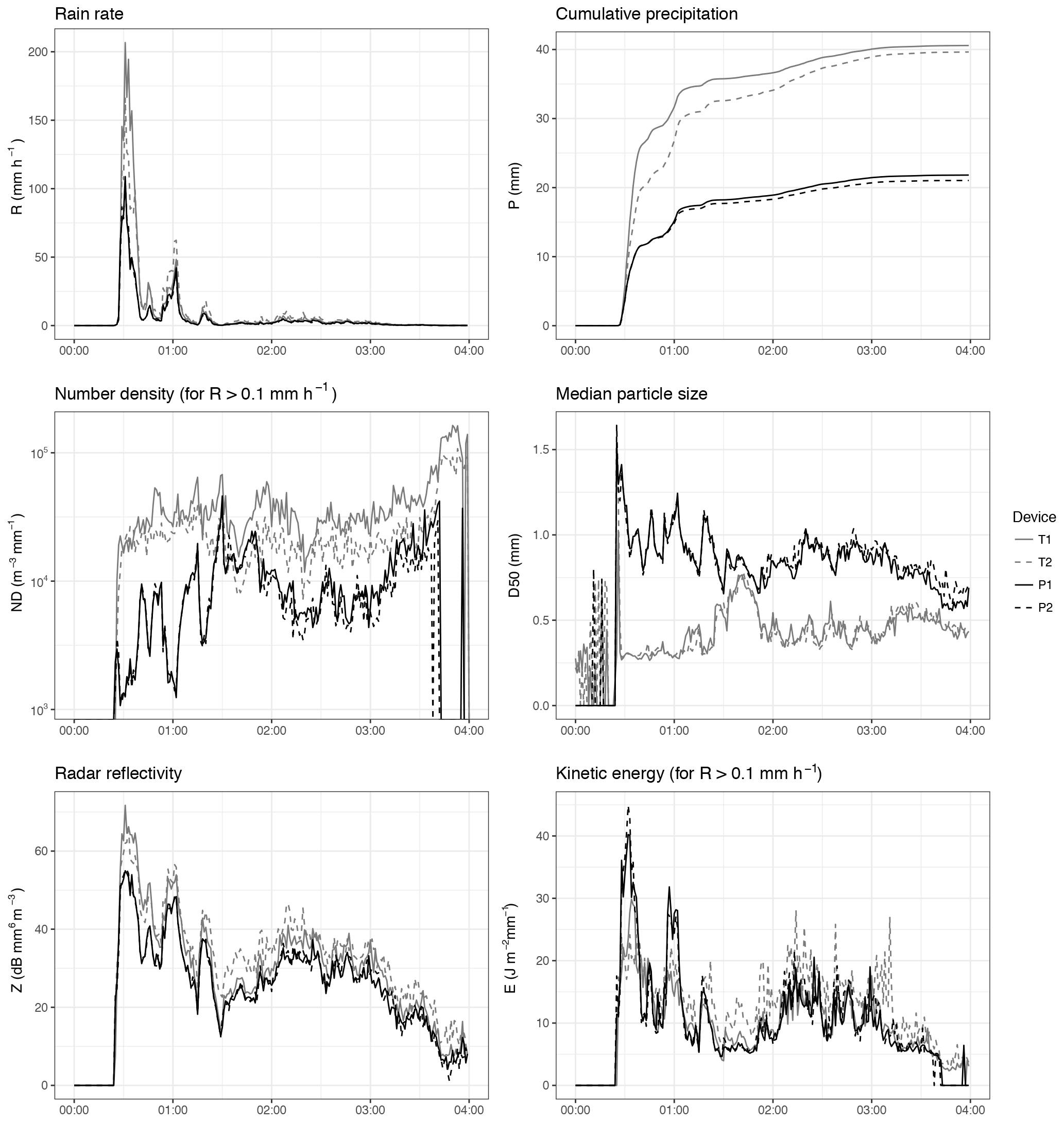
Figure A1Time series of disdrometer bulk variables during a high-intensity event (E365), with no corrections of the PSVD data.
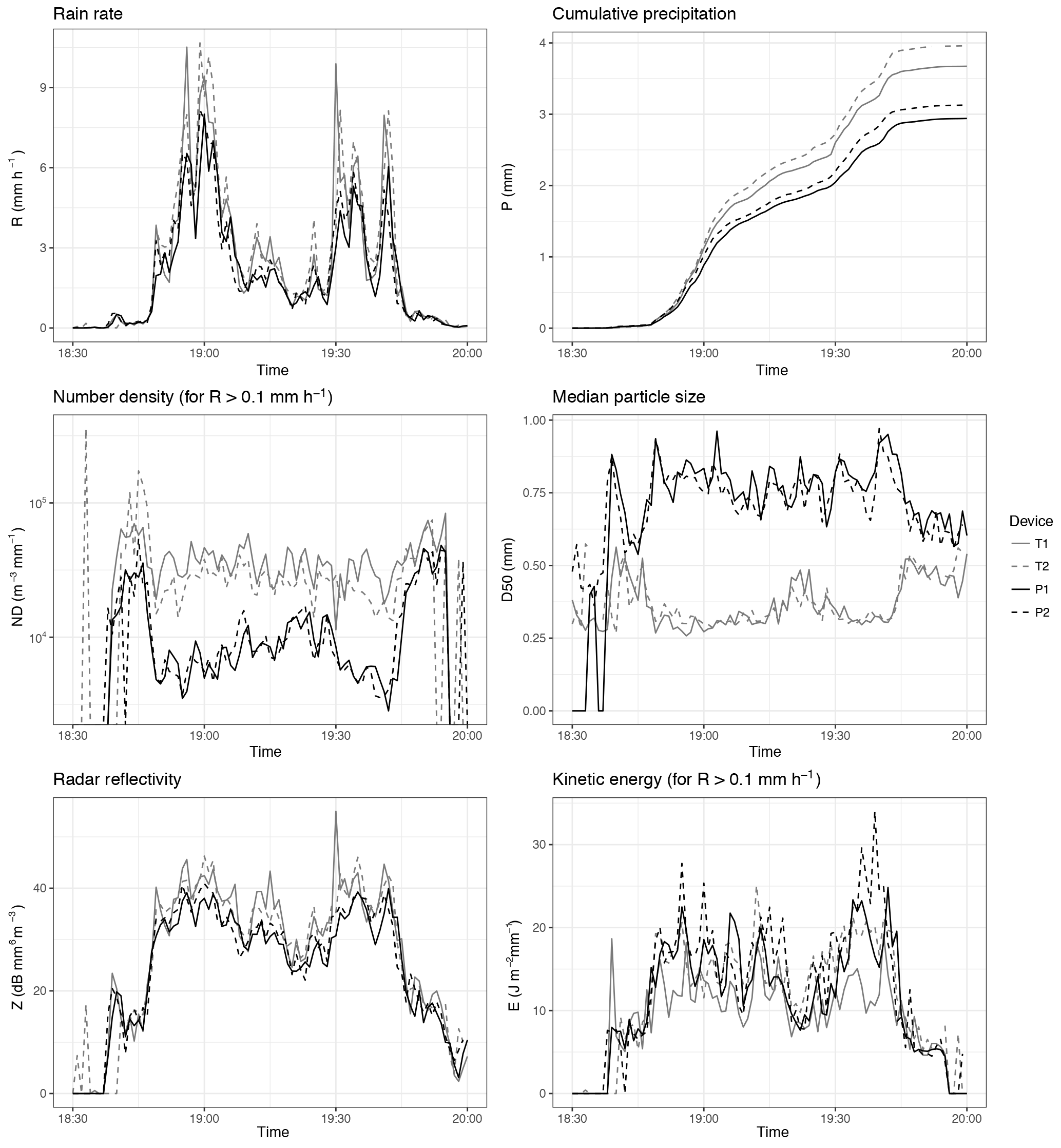
Figure A2Time series of disdrometer bulk variables during a low-intensity event (E455), with no corrections of the PSVD data.
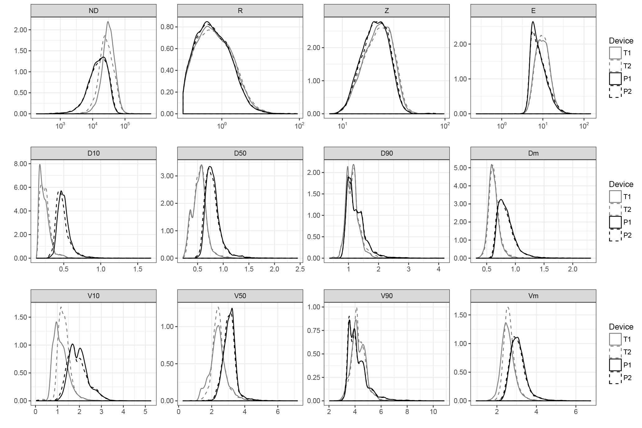
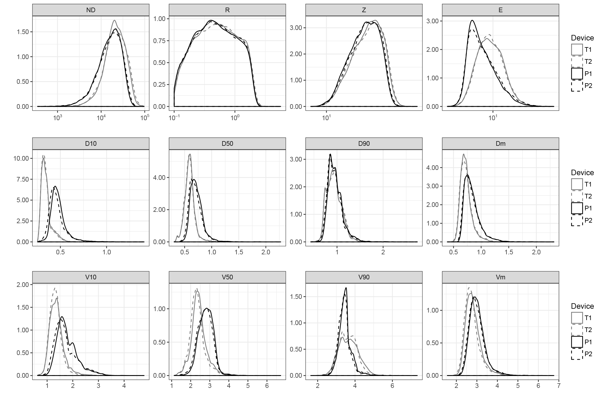
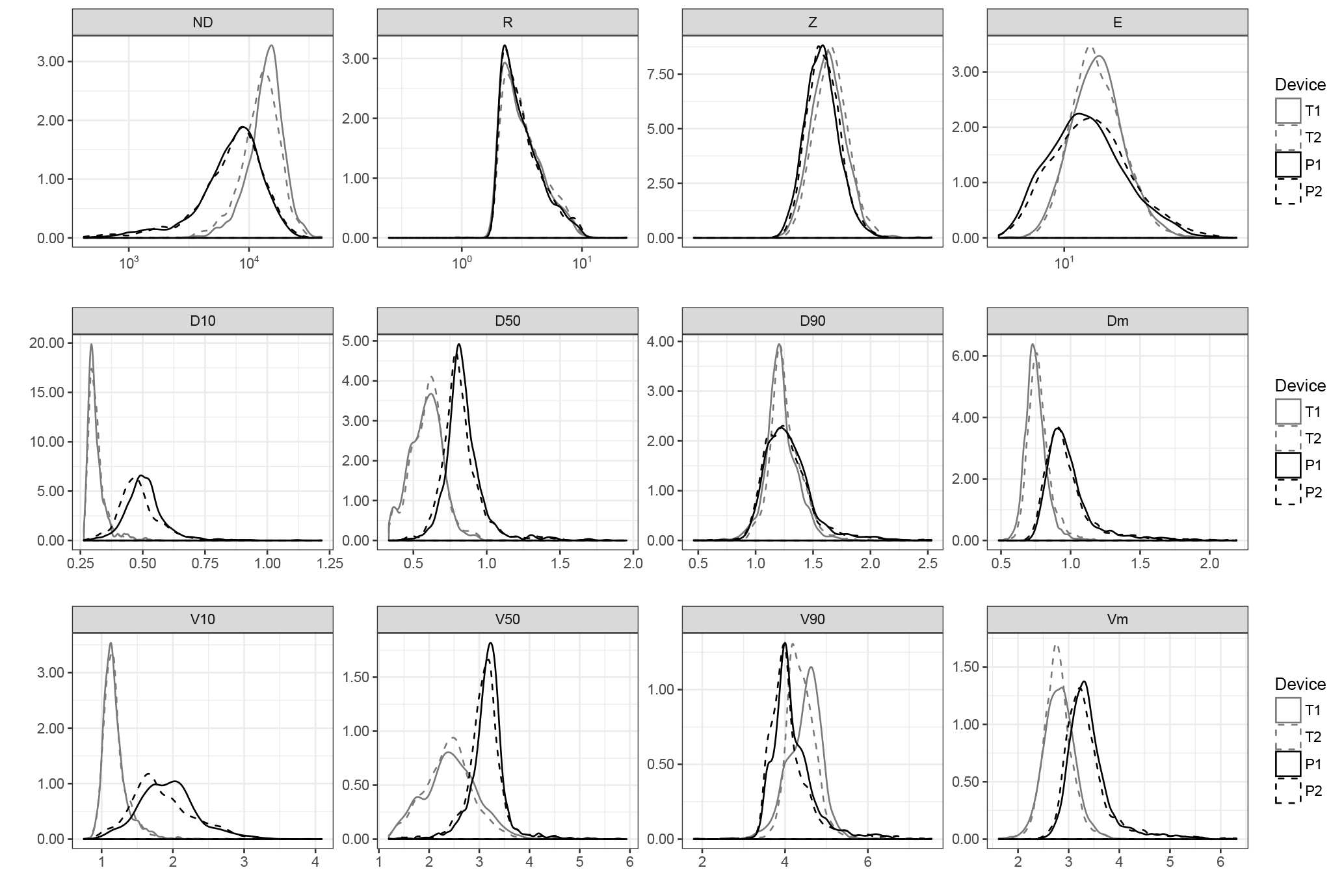
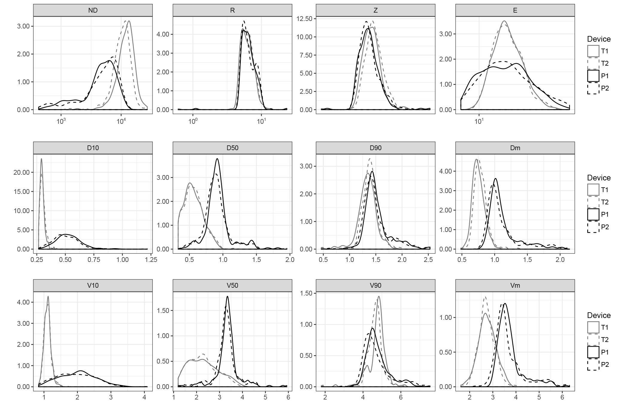
Table A1Gamma generalized linear mixed-effects model coefficients for 1 min records, with no corrections of the PSVD data (N=1000).
The authors declare that they have no conflict of interest.
This work has been supported by the research projects CGL2011-24185,
CGL2014-52135-C3-1-R and CGL2017-83866-C3-3-R, financed by the Spanish
Ministerio de Economía, Industria y Competitividad (MINECO) and EU-FEDER.
The work of Marta Angulo-Martínez was supported by a postdoctoral grant by
MINECO.
Edited by: Matjaz Mikos
Reviewed by: three anonymous referees
Adirosi, E., Baldini, L., Roberto, N., Gatlin, P., and Tokay, A.: Improvement of vertical profiles of raindrop size distribution from micro rain radar using 2D video disdrometer measurements, Atmos. Res., 169, 404–415, 2016.
Angulo-Martínez, M. and Barros, A. P.: Measurement uncertainty in rainfall kinetic energy and intensity relationships for soil erosion studies: An evaluation using Parsivel disdrometers in the Southern Appalachian Mountains, Geomorphology, 228, 28–40, 2015.
Angulo-Martínez, M., Beguería, S., Navas, A., and Machín, J.: Splash erosion under natural rainfall on three soil types in NE Spain, Geomorphology, 175–176, 38–44, 2012.
Angulo-Martínez, M., Beguería, S., and Kyselý, J.: Use of disdrometer data to evaluate the relationship of rainfall kinetic energy and intensity (KE-I), Sci. Total Environ., 568, 83–94, 2016.
Atlas, D., Ulbrich, C. W., Marks, J., Amitai, E., and Williams, C. R.: Systematic variation of drop size and radar-rainfall relations, J. Geophys. Res.-Atmos., 104, 6155–6169, 1999.
Battaglia, A., Rustemeier, E., Tokay, A., Blahak, U., and Simmer, C.: Parsivel snow observations: A critical assessment, J. Atmos. Ocean. Tech., 27, 333–344, 2010.
Beard, K. V.: Terminal velocity and shape of cloud and precipitation drops aloft, J. Atmos. Sci., 33, 851–864, 1976.
Beguería, S.: disdro-comparison: a dataset and code for comparing precipitation measurements by Ott Parsivel2 and Thies LPM optical disdrometers (Version v1.0), Zenodo, https://doi.org/10.5281/zenodo.1186413, 2018.
Beguería, S. and Latorre, B.: disdRo: an R package for working with disdrometric data (Version v0.3), Zenodo, https://doi.org/10.5281/zenodo.1186384, 2018.
Bloemink, H. I. and Lanzinger, E.: Precipitation type from the Thies disdrometer, WMO Technical Conference on Meteorological and Environmental Instruments and Methods of Observation (TECO- 2005), Bucharest, Romania, 4–7 May 2005, 3, 2005.
Brawn, D. and Upton, G.: On the measurement of atmospheric gamma drop-size distributions, Atmos. Sci. Lett., 9, 245–247, 2008.
Calheiros, A. J. P. and Machado, L. A. T.: Cloud and rain liquid water statistics in the CHUVA campaign. Atmos. Res., 144, 126–140, 2014.
Castro, A., Alonso-Blanco, E., González-Colino, M., Calvo, A. I., Fernández-Raga M., and Fraile, R.: Aerosol size distribution in precipitation events in León, Spain, Atmos. Res., 96, 421–435, 2010.
Ciaccioni, A., Bezak, N., and Rusjan, S.: Analysis of rainfall erosivity using disdrometer data at two stations in central Slovenia, Acta Hydrotechnica, 29, 89–101, 2010.
Cruse, R., Flanagan, D., Frakenberger, J., Gelder, B., Herzmann, D., James, D., Krajewski, W. F., Kraszewski, M., Laflen, J., Opsomer, J., and Todey, D.: Daily estimates of rainfall, water runoff, and soil erosion in Iowa, J. Soil Water Conserv., 61, 191–199, 2006.
Constantinescu, G. S., Krajewski, W. F., Ozdemir, C. E., and Tokyay, T.: Simulation of airflow around rain gauges: Comparison of LES with RANS models, Adv. Water Resour., 30, 43–58, 2007.
Donnadieu, G., Dubosclard, G., and Godard, S.: Un pluviometre photoelectrique pour la determination simultanee des espectres dimensionnel et de vitesse de chute des gouttes de pluie, J. Rech. Atmos., IV, 37–46, 1969.
Fernández-Raga, M., Fraile, R., Keizer, J. J., Varela Teijeiro, M. E., Castro, A., Palencia, C., Calvo, A. I., Koenders, J., and Da Costa Marques, R. L.: The kinetic energy of rain measured with an optical disdrometer: An application to splash erosion, Atmos. Res., 96, 225–240, 2010.
Frasson, R. P. D. M. and Krajewski, W. F.: Characterization of the drop-size distribution and velocity–diameter relation of the throughfall under the maize canopy, Agr. Forest Meteorol., 151, 1244–1251, 2011.
Frasson, R. P. D. M., da Cunha, L. K., and Krajewski, W. F.: Assessment of the Thies optical disdrometer performance, Atmos. Res., 101, 237–255, 2011.
Gires, A., Tchiguirinskaia, I., and Schertzer, D.: Multifractal comparison of the outputs of two optical disdrometers, Hydrolog. Sci. J., 61, 1641–1651, 2016.
Habib, E. and Krajewski, W. F.: An example of computational approach used for aerodynamic design of a rain disdrometer, J. Hydraul. Res., 39, 425–428, 2001.
Hauser, D., Amayenc, P., Nutten, B., and Waldteufel, P.: A new optical instrument for simultaneous measurement of raindrop diameter and fall speed distributions, J. Atmos. Ocean. Tech., 1, 256–269, 1984.
Iguchi, T., Kozu, T., Meneghini, R., Awaka, J., and Okamoto, K.: Rain-profiling algorithm for the TRMM precipitation radar, J. Appl. Meteorol., 39, 2038–2052, 2000.
Ioannidou, M. P., Kalogiros, J. A., and Stavrakis, A. K.: Comparison of the TRMM Precipitation Radar rainfall estimation with ground-based disdrometer and radar measurements in South Greece, Atmos. Res., 181, 172–185, 2016.
Iserloh, T., Ries, J., Arnáez, J., Boix-Fayos, C., Butzen, V., Cerdà, A., Echeverría, M., Fernandez-Gálvez, J., Fister, W., Geissler, C., Gómez, J., Gomez-Macpherson, H., Kuhn, N., Lazaro, R., León, Javier, Martínez-Mena, M., Martínez-Murillo, J., Marzen, M., Mingorance, M. D., and Wirtz, S.: European small portable rainfall simulators: A comparison of rainfall characteristics, Catena, 110, 100–112, 2013.
Jaffrain, J. and Berne, A.: Experimental quantification of the sampling uncertainty associated with measurements from Parsivel disdrometers, J. Hydrometeorol., 12, 352–370, 2011.
Jaffrain, J. and Berne, A.: Quantification of the small-scale spatial structure of the raindrop size distribution from a network of disdrometers, J. Appl. Meteorol. Clim., 51, 941–953, 2012.
Jameson, A. R. and Kostinski, A. B.: Fluctuation properties of precipitation. Part II: Reconsideration of the meaning and measurement of raindrop size distributions, J. Atmos. Sci., 55, 283–294, 1998.
Jameson, A. R., Larsen, M. L., and Kostinski, A. B.: Disdrometer network observations of finescale spatial-temporal clustering in rain, J. Atmos. Sci., 72, 1648–1666, 2015.
Jayawardena, A. W. and Rezaur, R. B.: Drop size distribution and kinetic energy load of rainstorms in Hong Kong, Hydrol. Process., 14, 1069–1082, 2000.
Joss, J. and Waldvogel, A.: Ein Spektrograph for Niederschlagstropfen mit automatischer Auswertung, PAGEOPH, 68, 240–246, 1967.
Kathiravelu, G., Lucke, T., and Nichols, P.: Rain Drop Measurement Techniques: A Review, Water, 8, 29, https://doi.org/10.3390/w8010029, 2016.
Krajewski, W. F., Kruger, A., and Nešpor, V.: Experimental and numerical studies of small-scale rainfall measurements and variability, Water Sci. Technol., 37, 131–138, 1998.
Krajewski, W. F., Kruger, A., Caracciolo, C., Golé, P., Barthes, L., Creutin, J.-D., Delahaye, J.-Y., Nikolopoulos, E. I., Ogden, F., and Vinson, J.-P.: DEVEX-disdrometer evaluation experiment: Basic results and implications for hydrologic studies, Adv. Water Resour., 29, 311–325, 2006.
Kruger, A. and Krajewski, W. F.: Two-dimensional video disdrometer: A description, J. Atmos. Ocean. Tech., 19, 602–617, 2002.
Lanza, L. G. and Vuerich, E.: The WMO field intercomparison of rain intensity gauges, Atmos. Res., 94, 534–543, 2009.
Lanzinger, E., Theel, M., and Windolph, H.: Rainfall amount and intensity measured by the Thies laser precipitation monitor WMO Technical Conf. on Meteorological and Environmental Instruments and Methods of Observation (TECO-2006), Geneva, Switzerland, 2006.
Liao, L., Meneghini, R., and Tokay, A.: Uncertainties of GPM DPR rain estimates caused by DSD parameterizations, J. Appl. Meteorol. Clim., 53, 2524–2537, 2014.
Lin, M., Lucas, H. C., and Shmueli, G.: Too big to fail: Large samples and the p-value problem, Inform. Syst. Res., 24, 906–917, 2013.
Löffler-Mang, M. and Blahak, U.: Estimation of the equivalent radar reflectivity factor from measured snow size spectra, J. Appl. Meteorol., 40, 843–849, 2001.
Löffler-Mang, M. and Joss, J.: An optical disdrometer for measuring size and velocity of hydrometeors, J. Atmos. Ocean. Tech., 17, 130–139, 2000.
Loik, M. E., Breshears, D. D., Lauenroth, W. K., and Belnap, J.: A multi-scale perspective of water pulses in dryland ecosystems: Climatology and ecohydrology of the western USA, Oecologia, 141, 269–281, 2004.
Marzano, F. S., Cimini, D., and Montopoli, M.: Investigating precipitation microphysics using ground-based microwave remote sensors and disdrometer data, Atmos. Res., 97, 583–600, 2010.
Miriovsky, B. J., Bradley, A. A., Eichinger, W. E., Krajewski, W. F., Kruger, A., Nelson, B. R., Creutin, J.-D., Lapetite, J.-M., Lee, G. W., Zawadzki, I., and Ogden, F. L.: An experimental study of small-scale variability of radar reflectivity using disdrometer observations, J. Appl. Meteor., 43, 106–118, 2004.
Nanko, K., Hotta, N., and Suzuki, M.: Assessing raindrop impact energy at the forest floor in a mature Japanese cypress plantation using continuous raindrop-sizing instruments, J. Forest Res., 9, 157–164, 2004.
Nanko, K., Watanabe, A., HOTTa, N., and Suzuki, M.: Physical interpretation of the difference in drop size distributions of leaf drips among tree species, Agr. Forest Meteorol., 169, 74–84, 2013.
Nes̆por, V., Krajewski, W. F., and Kruger, A.: Wind-Induced Error of Raindrop Size Distribution Measurement Using a Two-Dimensional Video Disdrometer, J. Atmos. Ocean. Tech., 17, 1483–1492, 2000.
Olsen, R. L., Rogers, D. V., and Hodge, D. B.: The aRb Relation in the Calculation of Rain Attenuation, IEEE T. Antenn. Propag., 26, 318–329, 1978.
Park, S. G., Kim, H. L., Ham, Y. W., and Jung, S. H.: Comparative Evaluation of the OTT PARSIVEL2 Using a Collocated Two-Dimensional Video Disdrometer, J. Atmos. Ocean. Technol., 34, 2059–2082, 2017.
Petan, S., Rusjan, S., Vidmar, A., and Mikos, M.: The rainfall kinetic energy-intensity relationship for rainfall erosivity estimation in the mediterranean part of Slovenia, J. Hydrol., 391, 314–321, 2010.
Pinheiro, J. C. and Bates, D. M.: Mixed-effects models in S and S-PLUS, Springer, New York, 2000.
Raasch, J. and Umhauer, H.: Errors in the determination of particle size distributions caused by coincidences in optical particle counters, Part. Part. Syst. Char., 1, 53–58, 1984.
Raupach, T. H. and Berne, A.: Correction of raindrop size distributions measured by Parsivel disdrometers, using a two-dimensional video disdrometer as a reference, Atmos. Meas. Tech., 8, 343–365, https://doi.org/10.5194/amt-8-343-2015, 2015.
Raupach, T. H. and Berne, A.: Spatial interpolation of experimental raindrop size distribution spectra, Q. J. Roy. Meteor. Soc., 142, 125–137, 2016.
Salles, C., Sempere-Torres, D., and Creutin, J. D.: Characterisation of raindrop size distribution in Mediterranean climate: analysis of the variations on the Z-R relationship, Proceedings of the 29th Conference on Radar Meteorology AMS, Montreal, Canada, 1999.
Sánchez-Moreno, J. F., Mannaerts, C. M., Jetten, V., and Löffler-Mang, M.: Rainfall kinetic energy-intensity and rainfall momentum-intensity relationships for Cape Verde, J. Hydrol., 454–455, 131–140, 2012.
Schönhuber, M., Lammer, G., and Randeu, W. L.: The 2D-video-distrometer, in: Precipitation: Advances in measurement, estimation and prediction, Springer, Berlin, Heidelberg, 3–31, 2008.
Sempere-Torres, D., Porra, J. M., and Creutin, J. D.: Experimental evidence of a general description for raindrop size distribution properties, J. Geophys. Res., 103, 1785–1797, 1998.
Sheppard, B. E. and Joe, P. I.: Comparison of raindrop size distribution measurements by a Joss- Waldvogel disdrometer, a PMS 2DG spectrometer, and a POSS Doppler radar, J. Atmos. Ocean. Tech., 11, 874–887, 1994.
Shuttlewort, W. J.: Terrestrial Hydrometeorology, Wiley-Blackwell, Oxford, UK, 472 pp., 2012.
Tan, J., Petersen, W. A., and Tokay, A.: A novel approach to identify sources of errors in IMERG for GPM ground validation, J. Hydrometeorol., 17, 2477–2491, 2016.
Tapiador, F. J., Checa, R., and De Castro, M.: An experiment to measure the spatial variability of rain drop size distribution using sixteen laser disdrometers, Geophys. Res. Lett., 37, L16803, https://doi.org/10.1029/2010GL044120 2010.
Tapiador, F. J., Navarro, A., Moreno, R., Jiménez-Alcázar, A., Marcos, C., Tokay, A., Durán, L., Bodoque, J. M., Martín, R., Petersen, W. A., de and Castro, M.: On the Optimal Measuring Area for Pointwise Rainfall Estimation: A Dedicated Experiment with 14 Laser Disdrometers, J. Hydrometeorol., 18, 753–760, 2017a.
Tapiador, F. J., Navarro, A., Levizzani, V., García-Ortega, E., Huffman, G. J., Kidd, C., Kucera, P. A., Kummerow, C. D., Masunaga, H., Petersen, W. A., Roca, R., and Sánchez, J. L.: Global precipitation measurements for validating climate models, Atmos. Res., 197, 1–20, 2017b.
Testud, J., Oury, S., Black, R. A., Amayenc, P., and Dou, X.: The concept of normalized distribution to describe raindrop spectra: A tool for cloud physics and cloud remote sensing, J. Appl. Meteorol., 40, 1118–1140, 2001.
Thurai, M. and Bringi, V. N.: Rain microstructure from polarimetric radar and advanced disdrometers, Precipitation: Advances in Measurement, Estimation and Prediction, edited by: Michaelides, S., Springer, Berlin, Heidelberg, 233–284, 2008.
Thurai, M., Petersen, W. A., Tokay, A., Schultz, C., and Gatlin, P.: Drop size distribution comparisons between Parsivel and 2-D video disdrometers, Adv. Geosci., 30, 3–9, https://doi.org/10.5194/adgeo-30-3-2011, 2011.
Thurai, M., Gatlin, P., Bringi, V. N., Petersen, W., Kennedy, P., Notaroš, B., and Carey, L.: Toward completing the raindrop size spectrum: Case studies involving 2D-video disdrometer, droplet spectrometer, and polarimetric radar measurements, J. Appl. Meteorol. Clim., 56, 877–896, 2017.
Tokay, A., Kruger, A., and Krajewski, W. F.: Comparison of drop size distribution measurements by impact and optical disdrometers, J. Appl. Meteorol., 40, 2083–2097, 2001.
Tokay, A., Petersen, W. A., Gatlin, P., and Wingo, M.: Comparison of raindrop size distribution measurements by collocated disdrometers, J. Atmos. Ocean Tech., 30, 1672–1690, 2013.
Tokay, A., Wolff, D. B., and Petersen, W. A.: Evaluation of the new version of the laser-optical disdrometer, OTT Parsivel2, J. Atmos. Ocean. Tech., 31, 1276–1288, 2014.
Uijlenhoet, R. and Sempere-Torres, D.: Measurement and parameterization of rainfall microstructure, J. Hydrol., 328, 1–7, 2006.
Ulbrich, C. W.: Natural variations in the analytical form of the raindrop size distribution, J. Clim. Appl. Meteorol., 22, 1764–1775, 1983.
Upton, G. and Brawn, D.: An investigation of factors affecting the accuracy of Thies disdrometers, WMO Technical Conference on Instruments and Methods of Observation (TECO-2008), St. Petersburg, Russian Federation, 27–29, 2008.
Zhang, L., Zhao, L., Xie, C., Liu, G., Gao, L., Xiao, Y., Shi, J., and Qiao, Y.: Intercomparison of Solid Precipitation Derived from the Weighting Rain Gauge and Optical Instruments in the Interior Qinghai-Tibetan Plateau, Adv. Meteorol., 2015, 936724, https://doi.org/10.1155/2015/936724, 2015.