Predicting groundwater recharge for varying land cover and climate conditions – a global meta-study

Groundwater recharge is one of the important factors determining the groundwater development potential of an area. Even though recharge plays a key role in controlling groundwater system dynamics, much uncertainty remains regarding the relationships between groundwater recharge and its governing factors at a large scale. Therefore, this study aims to identify the most influential factors of groundwater recharge, and to develop an empirical model to estimate diffuse rainfall recharge at a global scale. Recharge estimates reported in the literature from various parts of the world (715 sites) were compiled and used in model building and testing exercises. Unlike conventional recharge estimates from water balance, this study used a multimodel inference approach and information theory to explain the relationship between groundwater recharge and influential factors, and to predict groundwater recharge at 0.5^∘ resolution. The results show that meteorological factors (precipitation and potential evapotranspiration) and vegetation factors (land use and land cover) had the most predictive power for recharge. According to the model, long-term global average annual recharge (1981–2014) was 134 mm yr⁻¹ with a prediction error ranging from −8 to 10 mm yr⁻¹ for 97.2 % of cases. The recharge estimates presented in this study are unique and more reliable than the existing global groundwater recharge estimates because of the extensive validation carried out using both independent local estimates collated from the literature and national statistics from the Food and Agriculture Organization (FAO). In a water-scarce future driven by increased anthropogenic development, the results from this study will aid in making informed decisions about groundwater potential at a large scale.

1 Introduction

Human intervention has dramatically transformed the planet's surface by altering land use and land cover and consequently the hydrology associated with it. In the last 100 years the world population has quadrupled, from 1.7 billion (in 1900) to more than 7.3 billion (in 2014), and is expected to continue to grow significantly in the future (Gerland et al., 2014). During the last century, rapid population growth and the associated shift to a greater proportion of irrigated food production led to an increase in water extraction by a factor of ∼ 6. This eventually resulted in the overexploitation of both surface and groundwater resources, including the depletion of 21 of the world's 37 major aquifers (Richey et al., 2015). This depletion threatened human lives in many ways, ranging from critical reductions in water availability to natural disasters such as land subsidence (Chaussard et al., 2014; Ortiz-Zamora and Ortega-Guerrero, 2010; Phien-Wej et al., 2006; Sreng et al., 2009). Therefore, there is a need to closely examine approaches for sustainably managing this resource by controlling withdrawal from the system.

Groundwater recharge is one of the most important limiting factors for groundwater withdrawal and determines the groundwater development potential of an area (Döll and Flörke, 2005) Groundwater recharge connects atmospheric, surface and subsurface components of the water balance and is sensitive to both climatic and anthropogenic factors (Gurdak, 2008; Herrera-Pantoja and Hiscock, 2008; Holman et al., 2009; Jyrkama and Sykes, 2007). Various studies have employed different methods to estimate groundwater recharge including tracer methods, water table fluctuation methods, lysimeter methods and simple water balance techniques. Some of these studies input recharge to numerical groundwater models or dynamically link it to hydrological models to estimate variations under different climate and land cover conditions (Aguilera and Murillo, 2009; Ali et al., 2012; Herrera-Pantoja and Hiscock, 2008; Sanford, 2002).

In the last few decades, interest in global-scale recharge analysis has increased for various scientific and political reasons (Tögl, 2010). L'vovich (1979) made the first attempt at a global-scale analysis by creating a global recharge map using baseflow derived from river discharge hydrographs. The next large-scale groundwater recharge estimate was done by Döll (2002) who modelled global groundwater recharge at a spatial resolution of 0.5⁰ using the WaterGAP Global Hydrological model (WGHM; Alcamo et al., 2003; Döll, 2002). In this study, the runoff was divided into fast surface runoff, slow subsurface runoff and recharge using a heuristic approach. This approach considered relief, soil texture, hydrogeology and occurrence of permafrost and glaciers for the runoff partitioning. However, WGHM failed to reliably estimate recharge in semi-arid regions (Döll, 2002). Importantly, in that study, there was no consideration of the influence of vegetation which has been reported to be the second most important determinant of recharge by many researchers (Jackson et al., 2001; Kim and Jackson, 2012; Scanlon et al., 2005). In subsequent years, several researchers have attempted to model global groundwater recharge using different global hydrological models and global-scale land surface models (Koirala et al., 2012; Scanlon et al., 2006; Wada et al., 2010).

Although a fair amount of research has been carried out to model groundwater recharge at a global scale, most studies compared results to country-level groundwater information from the FAO (FAO, 2005). FAO statistics were based on estimates compiled from national institutions. The data estimation and reporting capacities of national agencies vary significantly and raise concerns about the accuracy of the data (Kohli and Frenken, 2015). In addition, according to FAO AQUASTAT reports, most national institutions in developing countries prioritise subnational-level statistics over national-level statistics, and in most cases data are not available for all subnational entities. This decreases the accuracy of country-wide averages and raises concerns about the reliability of using them as standard comparison measures. Only a few studies have validated modelled estimates against small-scale recharge measurements. Döll and Fiedler (2008) used 51 recharge observations from arid and semi-arid regions to correct model outputs. This study develops a recharge model and undertakes a more extensive validation of it using 715 local recharge measurements. Moreover, previous research has mostly been restricted to studying meteorological influences on recharge, few studies have systematically explored global-scale factors governing recharge. Much uncertainty still exists about the relationship between groundwater recharge and topographical, lithological and vegetation factors. Without adequate knowledge of these controlling factors, our capacity to sustainably manage groundwater globally will be seriously compromised.

The major objectives of this study are to identify the most influential factors of groundwater recharge and to develop an empirical model to estimate diffuse rainfall recharge. Specifically, to quantify regional effects of meteorological, topographical, lithological and vegetation factors on groundwater recharge using data from 715 globally distributed sites. These relationships are used to build an empirical groundwater recharge model and then the global groundwater recharge is modelled at a spatial resolution of 0.5^∘ × 0.5^∘ for the time period 1981–2014.

2 Methods

2.1 Dataset

This study is based on a compilation of recharge estimates reported in the literature from various parts of the world. This dataset is an expansion of previously collated sets of recharge studies along with the addition of new recharge estimates (Döll and Flörke, 2005; Edmunds et al., 1991; Scanlon et al., 2006; Tögl, 2010; Wang et al., 2010). The literature search was carried out using Google Scholar, Scopus and Web of Science with related keywords “groundwater recharge”, “deep percolation”, “diffuse recharge” and “vertical groundwater flux”. Several criteria were considered in including each study. To ensure that the data reflects all seasons, recharge estimates for time periods less than 1 year were excluded. The sites with significant contribution to groundwater from streams or by any artificial means were also eliminated as the scope of this research was to model naturally occurring recharge. In order to maximise the realistic nature of the dataset, all studies using some kind of recharge modelling were removed from the dataset. After all exclusions, 715 data points spread across the globe remained (Fig. 1) and were used for further analysis. Of these studies, 345 were estimated using the tracer method, 123 using the water balance method and the remaining studies used baseflow method, lysimeter or water table fluctuation method. This diversity in recharge estimation has enabled us to evaluate systematic differences in various measurement techniques. The year of measurement or estimation of recharge estimates in the final dataset differed (provided as supplementary material), and ranged from 1981 to 2014 (Fig. 2a). This inconsistency in the data raised a challenge when choosing the time frame for factors in the modelling exercise, particularly those showing inter-annual variation. Moreover, the compiled dataset does not represent all climate zones well (Fig. 2c), as most of the studies used were done either in arid, semi-arid or temperate zones. Pasture and cropland were the dominant land uses in the dataset (Fig. 2b).

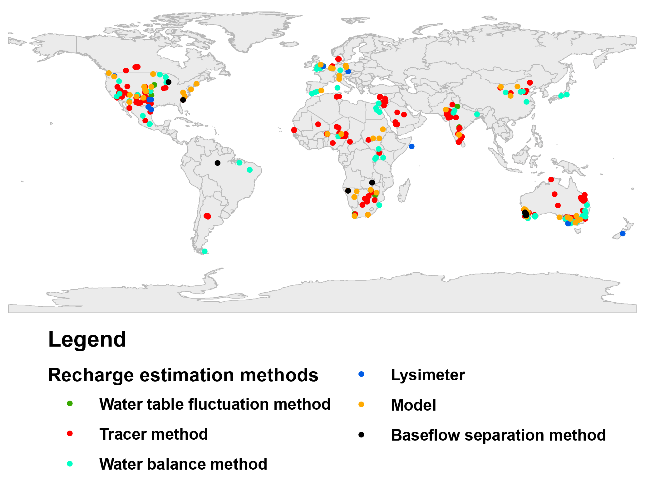
Figure 1 Locations of the 715 selected recharge estimation sites and the corresponding recharge estimation method, used for model building.

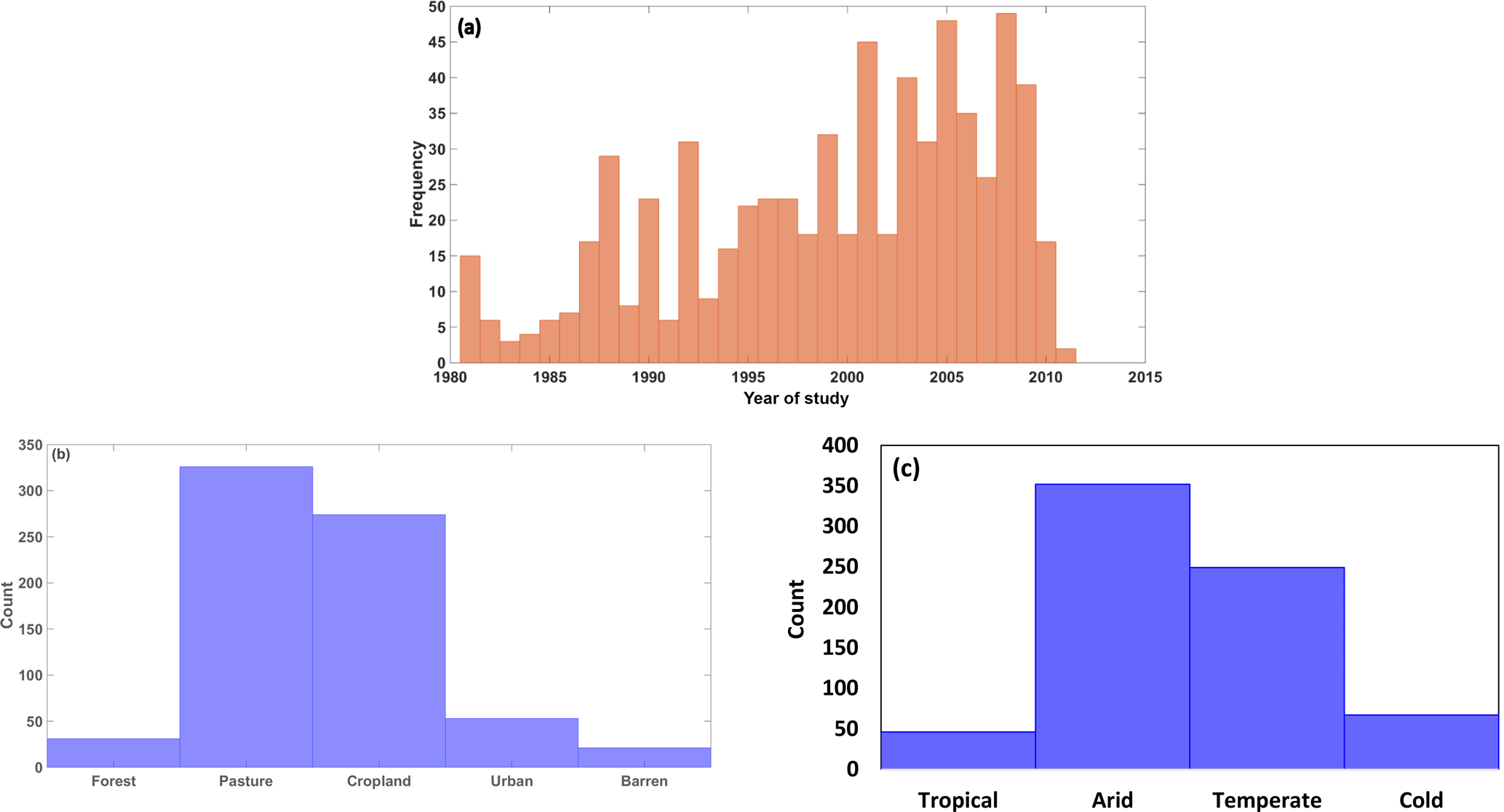
Figure 2 Histograms showing frequency of (a) study year, (b) land use and (c) Köppen–Geiger climate zones for the recharge estimates used.

Table 1 Description of predictors used for recharge model building.

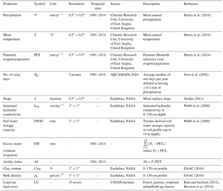
The next step was to identify potential explanatory factors that could influence recharge (henceforth referred to as predictors). Potential predictors that were reported in the literature as having some influence on recharge were identified (Athavale et al., 1980; Bredenkamp, 1988; Edmunds et al., 1991; Kurylyk et al., 2014; Nulsen and Baxter, 1987; O'Connell et al., 1995; Pangle et al., 2014). The choice of predictors was made based on the availability of global gridded datasets and their relative importance in a physical sense, as informed by the literature. According to the literature, the water availability on the surface for infiltration and the potential of the subsurface system to intake water are the two major controls on recharge. Different variables that can potentially represent these two factors were chosen as predictors in this study. The water availability is represented mainly by using meteorological predictors including precipitation, potential evapotranspiration, aridity index and number of days with rainfall and vegetation characteristics (land use and land cover), whereas the intake potential is represented using various quantifiable characteristics of the vadose zone. We employed 12 predictors comprising meteorological factors, soil/vadose zone factors, vegetation factors and topographic factors. However, other factors which could have a sizable influence on recharge were not included in this study because of insufficient data. Thus, we did not consider the effects of irrigation on recharge, limiting the scope of the study to rainfall-induced recharge. Subsurface lithology which could be another important recharge factor, was also eliminated from the study, due to a lack of suitable lithological and geological datasets at a larger scale. Better quality information about various predictors would have been desirable to enhance the accuracy of prediction. Details of predictors are given in Table 1.

Data for the chosen predictors corresponding to 715 recharge study sites were extracted from global datasets. Meteorological datasets (P, T and PET) were obtained from the Climatic Research Unit, University of East Anglia, United Kingdom. Even though daily data were available from 1901 to 2014 at a resolution of 0.5^∘ × 0.5^∘, in this study the mean annual average of the latest 34 years (1981 to 2014) was used to reduce the inconsistency in year of recharge measurements in the final dataset. Topographic and soil data were acquired from the NASA Earth observation dataset. Both datasets were of 0.5^∘ × 0.5^∘ spatial resolution. A few of the predictors, including number of rainfall days (R_d) and land use/land cover (LU) data were obtained from AquaMaps (by FAO) and USGS (United States Geological Survey) at a spatial resolution of 0.5^∘ × 0.5^∘ and 15 arcmin respectively. Thus-obtained LU data were compared with land cover reported in literature and corrected for any discrepancies. The spatial resolution of the different data used was diverse. This was dealt with by extracting the values for each recharge site from the original grids using the nearest neighbour interpolation method. As a result, predictor data extracted for each recharge site will differ from the actual value due to scaling and interpolation errors. Out of the 12 predictors LU was not a quantitative predictor and was transformed into a categorical variable in the modelling exercise.

2.2 Recharge model development

With empirical studies, the science world is always sceptical about whether to use a single best-fit model or to infer results from several better-predicting and plausible models. The former option is feasible only if there exists a model which clearly surpasses other models, which is rare in the case of complex systems like groundwater. Usually cross correlation and multiple controlling influences on the system lead to more than one model having similarly good fits to the observations. Thus choosing explanatory variables and model structure is a significant challenge. In the past this challenge was often addressed using various step-wise model construction methods, with the final model being selected based on some model fit criteria that penalise model complexity (Fenicia et al., 2008; Gaganis and Smith, 2001; Jothityangkoon et al., 2001; Sivapalan et al., 2003). These approaches were pragmatic responses to the large computational load involved in trying all possible models. The disadvantage of this method is that the final model will be dependent on the step-wise selection process used (Sivapalan et al., 2003). An alternative approach for addressing this high level of uncertainty in model structure is to adopt a multi-model inference approach that compares many models (Duan et al., 2007; Poeter and Anderson, 2005). It typically results in multiple final models and an assessment of the importance of each explanatory variable. Therefore, this approach was used to develop an understanding of the role of different controlling factors on recharge in a data-limited condition.

Choosing predictors that are capable of representing the system and selecting the right models for prediction are the key steps in the multi-model inference approach. Here, models were chosen by ranking the fitted models based on performance, and comparing this to the best-performing model in the set (Anderson and Burnham, 2004). This model ranking also provided a basis for selecting individual predictors. The analysis progressed through three key stages: exploratory analysis, model building and model testing.

2.2.1 Multi-model analysis

A multi-model selection process aims to explore a wide range of model structures and to assess the predictive power of different models in comparison with others. Essentially, models with all possible combinations of selected predictors are developed and assessed via traditional model performance metrics (discussed later). By conducting such an exhaustive search, multi-model analysis avoids the problems associated with selection methods in step-wise regression approaches (Burnham and Anderson, 2003). Importantly, it reduces the chance of missing combinations of predictors with good predictive performance. However, a disadvantage of this approach is that the number of predictor combinations grows rapidly with the number of factors considered. To make the analysis computationally efficient, we set an upper limit for the number of predictors used. Another problem with this approach is that it can result in overfitting. To address this issue we evaluated model performance with metrics that penalise complexity and tested the model robustness with a cross-validation analysis. The model development procedure using multi-model analysis is described in detail below.

(a) Exploratory analysis

Firstly, all the chosen predictors were individually regressed against the compiled recharge dataset. This was carried out with the main objective of finding the predictors with significant control over recharge and to gain an initial appreciation of how influential each predictor is compared to the others. This understanding will aid in eliminating the least influential predictors from further analysis. Then assumptions involved in regression analysis, such as linearity, low multicollinearity (important for later multivariate fitting) and independent identically distributed residuals were analysed using residual analysis. Following the residual analysis, various data transformations (square root, logarithmic and reciprocal) were carried out to reduce heteroscedasticity and improve linearity of the variables. The square root transformed recharge along with non-transformed predictors gave the most homoscedastic relationships (results not shown). Therefore, these transformed values were used in further model-building exercises. Predictors were selected and eliminated based on statistical indicators such as adjusted coefficient of determination ($R_{\mathrm{adj}}^{\mathrm{2}}$) value and root mean square error (RMSE).

(b) Model building

Multiple linear regression was employed for building the models as the transformed dataset did not exhibit any nonlinearity. Furthermore, the presence of both negative and positive values in the dataset restricted the applicability of other forms of regression analysis like log-linear and exponential (Saft et al., 2016). Linear regression is known for its simple and robust nature in comparison to higher-order analysis. The robustness of linear regression helped to maintain parsimony together with reasonable prediction accuracy. A rigorous model-building approach was adopted in order to capture the interplay between predictors with combined/interactive effects on groundwater recharge. This is an exhaustive search in which all candidate models are fitted and inter-compared using performance criteria. In a way, this modelling exercise used a top-down approach, starting with a simple model which is expanded as shortcomings were identified (Fenicia et al., 2008).

(c) Model testing

The analysis above provided insight into the relative performance of the models. However, it is also important to assess the dependence of the results on the particular sample. Therefore, we conducted a subsample analysis in which the same method was re-applied to subsamples of the data. Finally, predictive uncertainty was estimated through leave-one-out cross validation. In the first case, the whole model development process was redone multiple times using subsamples of the data. To achieve this, the entire dataset was randomly divided into 80 and 20 % subsets and 80 % of the data were used for building the model. The predictive performance of the developed model was tested against the omitted 20 % of data. This was repeated 200 times in order to eliminate random sampling error. The leave-one-out cross validation was applied to the best few individual model structures and provided an estimate of predictive performance for those particular models. It also gave an indication of data quality at each point.

In summary the key steps in the multi-model analysis were

1. selecting predictors;

2. fitting all possible models consisting different combinations of predictors;

3. calculating model performance metrics for each model;

4. calculating the “weight of evidence” for each predictor based on the performance metric of all models containing that predictor;

5. testing the predictive performance of the models.

2.2.2 Ranking models and predictors

This part of the analysis has closely followed the approach developed in Saft et al. (2016). Model performance was evaluated using several information criteria. These information criteria include a goodness-of-fit term and an overfitting penalty based on the number of predictors in the model. In this study we used $R_{\mathrm{adj}}^{\mathrm{2}}$, the consistent Akaike information criterion (AIC_c) and the complete Akaike information criterion (CAIC) as the performance evaluation criteria. These criteria differ in terms of penalising overfitting. $R_{\mathrm{adj}}^{\mathrm{2}}$ penalises overfitting the least, AIC_c moderately and CAIC heavily. However, when we are unsure of the true model and whether it overfits or not, there is some advantage in employing several criteria as it gives insight into how the results depend on the criteria used. Suitability of the information criteria also varies with the sample size. CAIC acts as an unbiased estimator for large sample size with relatively small candidate models, but produces large negative bias in other cases. Conversely, AIC_c is well suited for small-sample applications (Cavanaugh and Shumway, 1997; Hurvich and Tsai, 1989). The formulas for the above criteria are as follows:

$$\begin{array}{}\text{(1)}& {\displaystyle }{\displaystyle }\mathrm{AIC}=-\mathrm{2}\times \mathrm{llf}+\mathrm{2}\times k(\mathrm{Akaike},\mathrm{1974}),\end{array}$$

$$\begin{array}{ll}{\displaystyle }{\mathrm{AIC}}_{\mathrm{c}}=& {\displaystyle }\mathrm{AIC}+(\mathrm{2}\times (k-\mathrm{1})\times {\displaystyle \frac{k+\mathrm{2}}{n-k-\mathrm{2}}})(\mathrm{Hurvich}\mathrm{and}\\ \text{(2)}& {\displaystyle }& {\displaystyle }\mathrm{Tsai},\mathrm{1989}),\end{array}$$

$$\begin{array}{}\text{(3)}& {\displaystyle }{\displaystyle }\mathrm{CAIC}=-\mathrm{2}\times \mathrm{llf}+k\times \left(\ln \right(n)+\mathrm{1})(\mathrm{Bozdogan},\mathrm{1987}),\end{array}$$

$$\begin{array}{ll}{\displaystyle }{R}^{\mathrm{2}}=& {\displaystyle }\mathrm{1}-\left[{\displaystyle \frac{n-\mathrm{1}}{n-k-\mathrm{1}}}\right]\times \left[\mathrm{1}-R^{\mathrm{2}}\right](\mathrm{Ezekiel},\mathrm{1929};\\ \text{(4)}& {\displaystyle }& {\displaystyle }\mathrm{Wang}\mathrm{and}\mathrm{Thompson},\mathrm{2007}),\end{array}$$

where “llf” is the log-likelihood function, k is the dimension of the model and n is the number of observations.

When assessing candidate models there are two questions which are of particular interest. (1) Which models are better? (2) How much evidence exists for each predictor in predicting recharge? Analysis of the AIC_c and CAIC was used to answer both these questions. Models were ranked using information criteria, with smaller values indicating better performance. Information criteria are more meaningful when they are used to evaluate the relative performance of the models (Poeter and Anderson, 2005). Models were ranked from best to worst by calculating model delta values (Δ) and model weights (W) as follows:

$$\begin{array}{}\text{(5)}& {\displaystyle }& {\displaystyle }{\mathrm{\Delta }}_i={\mathrm{AIC}}_i-{\mathrm{AIC}}_{\min },\text{(6)}& {\displaystyle }& {\displaystyle }{W}_i=\exp \left(-\mathrm{0.5}\times {\mathrm{\Delta }}_i\right)/\mathrm{\Sigma }\exp \left(-\mathrm{0.5}\times {\mathrm{\Delta }}_m,\right)\end{array}$$

where AIC_min is the information criteria value of the best model. Δ_i and W_i represent the performance of ith model in comparison with the best-performing model in the set of M models.

Evidence ratios were then calculated as the ratio of the ith model weight to the best model weight. They can be used as a measure of the evidence for the ith model compared to the other models. They also provide means to estimate the importance of each predictor. This involves transformation of evidence ratios into a proportion of evidence (PoE) for each predictor. PoE for a predictor is defined as the sum of weights of all the models containing that particular predictor. PoE ranges from 0 to 1. The closer the PoE of a predictor is to 1, the more influential that predictor is.

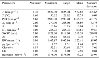
Table 2 Summary statistics of potential predictors from the dataset used in this study.

2.3 Global groundwater recharge estimation

The best model (model 1, Table 3) from the above analysis was used to build a global recharge map at a spatial resolution of 0.5^∘ × 0.5^∘. Recharge estimation was done annually for a study period of 34 years (1981–2014), and the estimated groundwater recharge was then averaged over the 34-year period to produce a global map. In addition to this, maps showing percentage of rainfall becoming recharge and the standard deviation of annual recharge over the 34 years were also generated. As recharge data from regions with frozen soil were scarce in the model-building dataset, the model predictions in those regions particularly for regions with Köppen–Geiger classification Dfc, Dfd, ET and EF were not highly reliable. EF regions of Greenland and Antarctica were excluded from the final recharge map due to lack of both recharge and predictor data. However, the modelled recharge for Dfc, Dfd and ET regions were included because of the availability of predictor data. In addition, the modelled recharge values were compared against country-level statistics from FAO (2005) for 153 countries.

3 Results

The results address three important questions. (1) What are the most influential predictors of groundwater recharge? (2) What are better models for predicting recharge? (3) How does groundwater recharge vary over space and time? The first question was answered by carrying out an exploratory data analysis and also by estimating the PoE for each predictor, the second using information criteria and the third by mapping recharge at 0.5^∘ × 0.5^∘ using the best model.

Figure 3 Model fit performance criteria for single predictor regressions.

3.1 Exploratory data analysis

Table 2 gives the statistical summary of predictors and groundwater recharge at 715 data sites. It is apparent from the table that predictors varied considerably between sites, consistent with inter-site variability in regional physical characteristics. This variability provided an opportunity to explore recharge mechanisms in a range of different physical environments. As we used linear regression to study the one-to-one relationship of recharge with each of the predictors, RMSE and bias of fitting were used to identify the predictors with the most explanatory power. In this case, RMSE values ranged between 23.2 mm yr⁻¹ for P and 30.21 mm yr⁻¹ for S. Predictive potential of meteorological predictors was greater than for other classes of predictor (Fig. 3). P, AI, EW and ρ_b had a negative bias, whereas all other predictors had a positive bias.

Table 3 Coefficient of predictors used in the top 10 models, ranked based on CAIC.

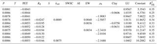
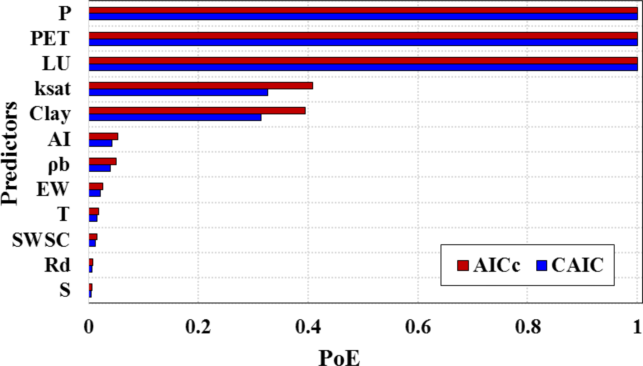
Figure 4 Proportion of evidence according to AIC_c and CAIC for 12 predictors (sorted in descending order of PoE).

3.2 Multi-model analysis

3.2.1 Proportion of evidence (PoE) for individual predictors

Figure 4 shows the PoE of the 12 predictors used in this study. According to this analysis, 3 of the 12 predictors stood out as having the greatest explanatory power (Fig. 4). Precipitation (P), potential evapotranspiration (PET) and land use and land cover (LU) had the highest proportions of evidence (∼ 1). Subsurface percentage of clay (clay) and saturated hydraulic conductivity (k_sat) also had an important influence on recharge with PoE ∼ 0.4. Aridity index (AI), rainfall days (R_d), mean temperature (T), bulk density (ρ_d), slope (S), excess water (EW) and soil water storage capacity at root zone (SWSC) were in the lower PoE range (< 0.1 according to both the criteria). There was some variation in the PoE value of the predictors depending on the performance metric, due to the diversity in overfitting penalty. However, ranking of the variables was identical irrespective of the performance metric used. The “best” and “worst” predictors ranked according to $R_{\mathrm{adj}}^{\mathrm{2}}$ were also in agreement with the PoE analysis (not shown). In addition, results of the subsample analysis gave similar results (not shown).

3.2.2 Better-performing models

According to information criteria, the performance of models can only be evaluated relative to the best-performing model in the set. In this study, as per the model weights, no model exhibited apparent dominance. The evidence ratio (ratio between the weights of the best model and nth model) suggested that the best model according to CAIC was only 1.04 times better than the second best model. However, the evidence ratio increased exponentially with increase in model rank and there was a clear distinction between better models and worse models. Similar results were reported by Saft et al. (2016) in her work for modelling rainfall–runoff relationship shift. The choice of better models was made by considering the PoE of individual predictors (refer Sect. 3.2.1) and the number of predictors in the model (V). Figure 5 shows the performance criteria for the top three models for different V values. The model performance increased with V up to 6 to 7 depending on the different criteria. After that, AIC_c, CAIC, RMSE and $R_{\mathrm{adj}}^{\mathrm{2}}$ values remained almost constant, indicating that further addition of predictors did not improve the model performance. In particular CAIC shows reaches a minimum at V = 7 and it penalises model complexity more rigorously. Table 3 illustrates the predictors in the top 10 models selected based on CAIC. All the top 10 models had V $<=$ 7. P, PET and LU repeatedly appeared in the predictor list of the top 10 models substantiating their high predictive capacity, and the top ranked model includes these three predictors only. In this particular case, top-performing models according to both information criteria were the same; therefore results from only one criteria (CAIC) will be discussed.

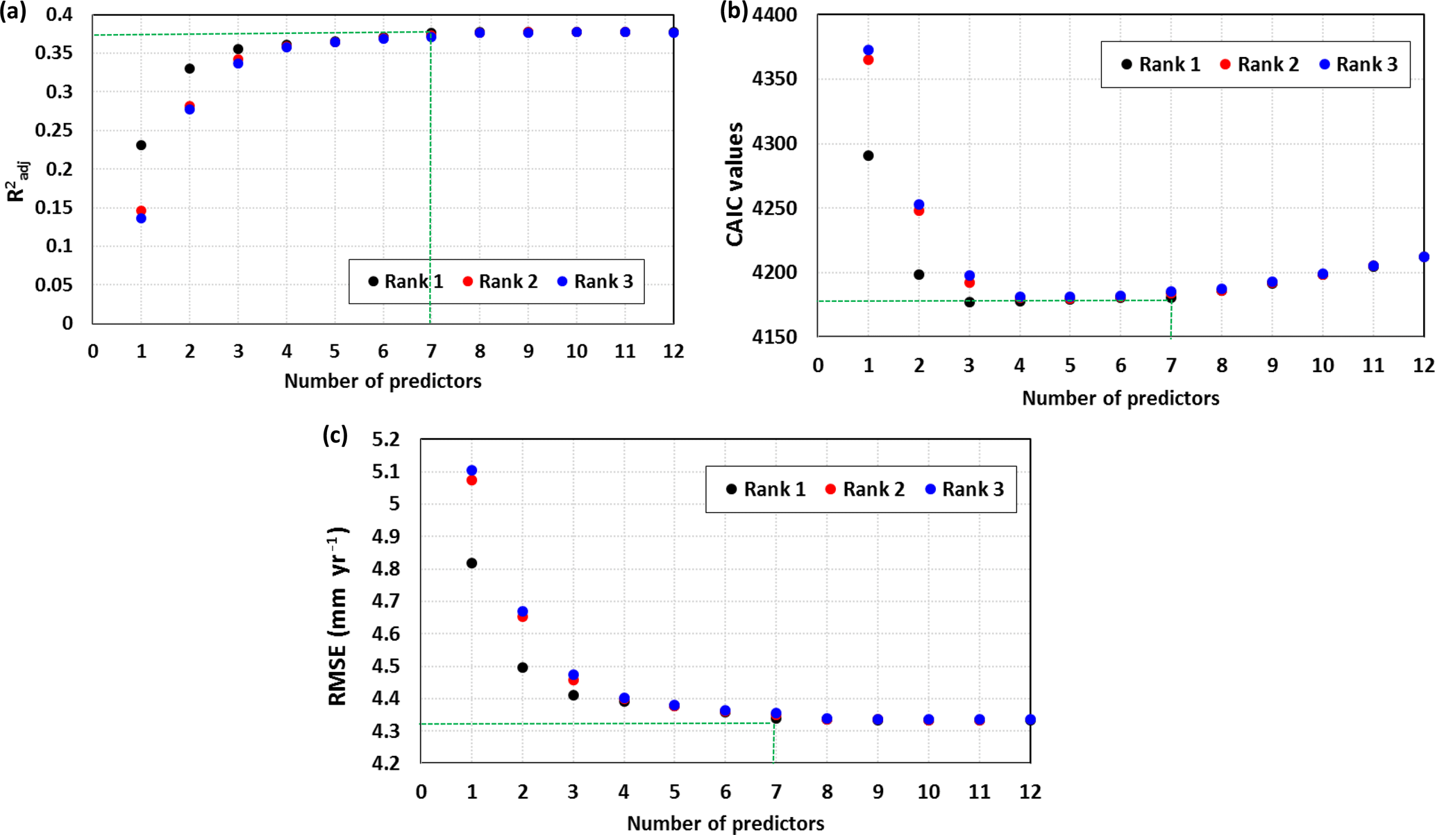
Figure 5 (a) $R_{\mathrm{adj}}^{\mathrm{2}}$, (b) CAIC and (c) RMSE for the top three models with 1 to 12 predictors and the green dotted lines representing the number of predictors for the best performance criteria value.

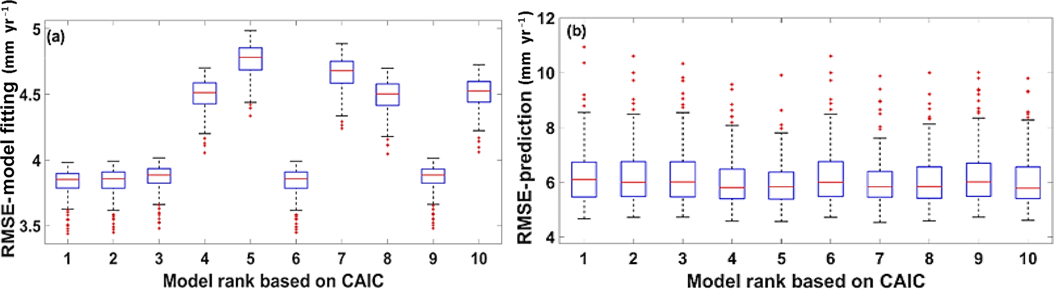
Figure 6 RMSE of sub-sample (a) model fitting and (b) model prediction of top 10 models according to CAIC.

3.2.3 Model testing

Models ranking from 1 to 10 according to CAIC (Table 3) were tested using both model testing techniques discussed in Sect. 2.2.1c. Figure 6 depicts model fit and model prediction RMSE values of 200 subsample tests. It is clear from the box plots that the difference between the RMSE of the 1st and the 10th model during both model fitting and prediction is less than 1 mm yr⁻¹. In subsample tests, $R_{\mathrm{adj}}^{\mathrm{2}}$ of the best model ranged from 0.42 to 0.56 implying 42 to 56 % of the variance was explained (please see Sect. 3.2.3 for details on sub-sample testing). The model errors at each data point ranged from −8 to 28 mm yr⁻¹. However, 97.2 % of the points had errors between −8 and 10 mm yr⁻¹. Figure 7 shows the relationship between precipitation and model errors and it is evident from this scatter plot that model predictions were not greatly influenced by low or high precipitation. In other words, the model was unbiased by precipitation trends. Similar checking was done for all other predictors (not shown) which all showed a similar pattern to precipitation. The dataset was classified based on recharge estimation techniques and model performance was tested with results showing no systematic difference (not shown).

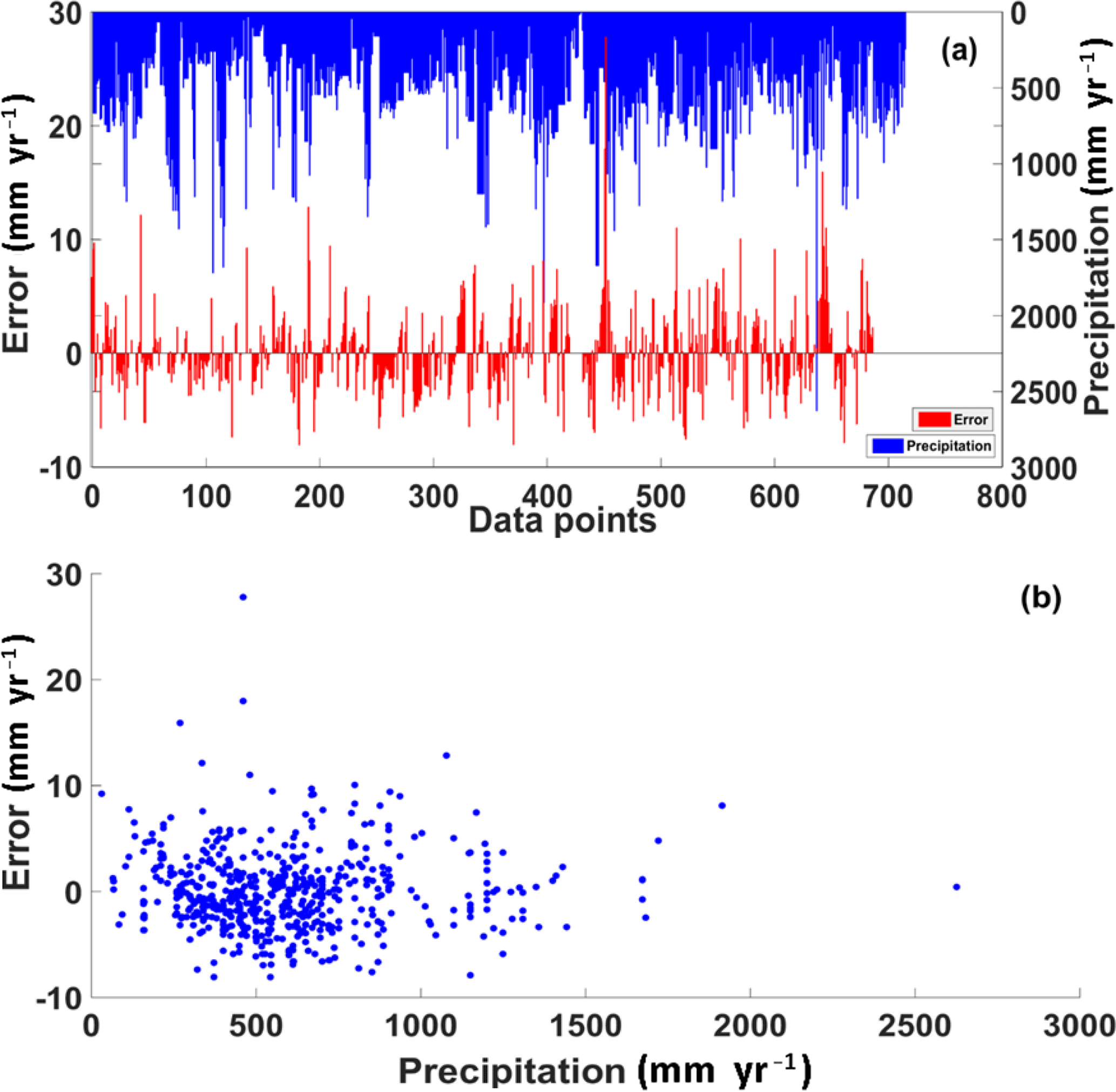
Figure 7 (a) Error at each data point along with the corresponding rainfall obtained using the leave-one-out model testing procedure and (b) Scatter plot between error at each data point and corresponding precipitation.

3.3 Global groundwater recharge

The global long term (1981–2014) mean annual groundwater recharge map at a spatial resolution of 0.5^∘ was made by the model developed in Sect. 3.2 (Fig. 8). In this study, the best model as defined by CAIC (model 1 in Table 3) was used to generate the recharge map. However, due to the similarity in structure of the top 10 models (Table 3), all models were equally good at predicting groundwater recharge and gave similar results (not shown). Grid-scale recharge ranged from 0.02 to 996.55 mm yr⁻¹ with an average of 133.76 mm yr⁻¹. The highest recharge was associated with very high rainfall (> 4000 mm yr⁻¹). Humid regions such as Indonesia, Philippines, Malaysia, Papua New Guinea, Amazon, western Africa, Chile, Japan and Norway had very high recharge (> 450 mm yr⁻¹), whereas arid regions of Australia, the Middle East and Sahara had very low recharge (< 0.1 mm yr⁻¹). In humid areas, percentage of rainfall becoming groundwater recharge (> 40 %) was found to be very high in comparison to other parts of the world. However, the mean percentage of rainfall becoming recharge is only 22.06 % across the globe. Among all the continents, Australia had the lowest annual groundwater recharge rate.

Over the 34 years, global annual mean recharge followed the same pattern as that of global annual mean precipitation (Fig. 9). Least recharge was predicted in the year 1987 (groundwater recharge = 95 mm yr⁻¹), where the annual average rainfall was < 180 mm yr⁻¹. Variation in recharge over the years was maximal in arid regions of Australia and North Africa (Fig. 10a). However, the standard deviation of recharge was higher in humid areas than in arid regions (Fig. 10b). This indicates that standard deviation did not clearly represent year-to-year variations in recharge. Potentially, the advantage of using coefficient of variation over standard deviation is that it can capture variations even when mean values are very small. In this case precipitation and potential evapotranspiration were the two major predictors of recharge. Globally, variability in evapotranspiration is much less than variability in rainfall (Peel et al., 2001; Trenberth and Guillemot, 1995). Therefore, variability of groundwater recharge both temporally and spatially is due to variability in precipitation, which implies that arid regions are more susceptible to inter-annual variation in groundwater recharge. A comparison of predicted recharge against country-level recharge estimates from FAO (2005) shows that the model tends to overpredict recharge, particularly for low recharge areas. However, due to inaccuracies in the FAO estimates this cannot be considered as a reliable comparison (Fig. 11a). Recharge estimates from the best models in the present study were compared to recharge estimates from the complex hydrological model (WaterGAP; Fig. 11b). Even though the model in this study overestimates recharge for countries with fewer data points, the scatter shows a smaller spread compared to the FAO estimates. Figure 12 shows the country-wide distribution of errors in model prediction in comparison with FAO statistics. Very high errors were found in countries with fewer model-building data points. The model considerably overestimated recharge for Russia, Canada, Brazil, Indonesia, Malaysia and Madagascar.

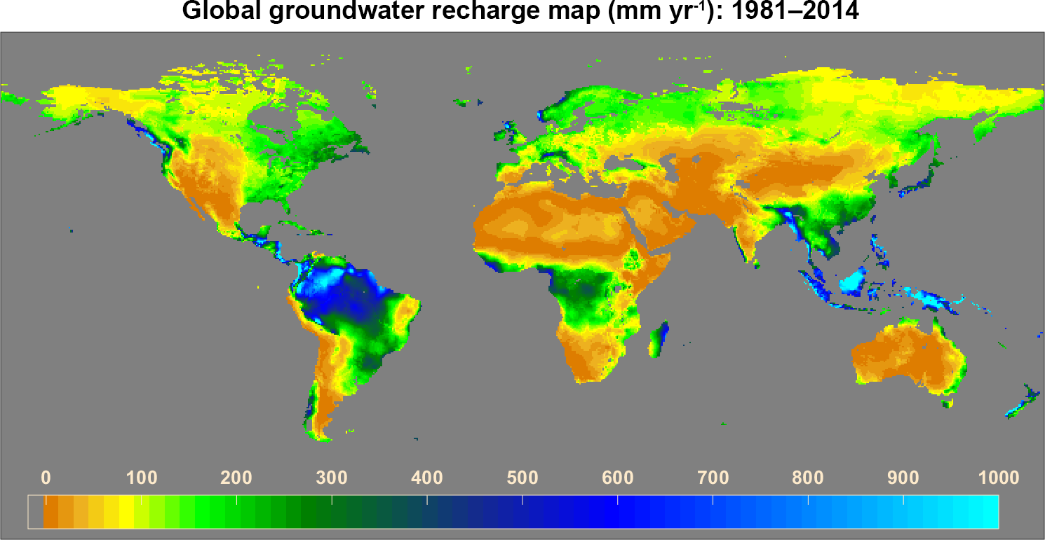
Figure 8 Long-term (1981–2014) average annual groundwater recharge estimated using the developed model.

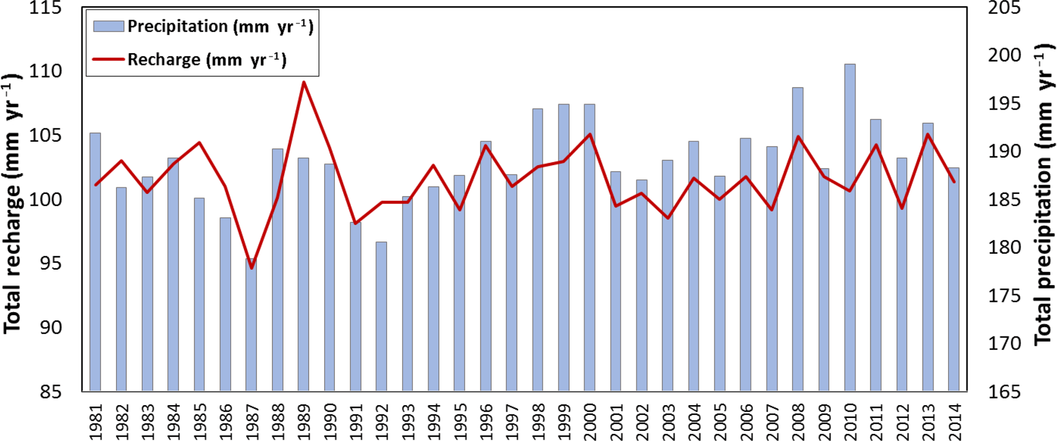
Figure 9 Temporal distribution of total global recharge along with total global precipitation of corresponding years for a period of 1981 to 2014.

4 Discussion

The aims of this study were to identify the factors with the most influence on groundwater recharge, and to develop a global model for predicting groundwater recharge under limited data conditions, without extensive water balancing. In this study, an empirical model-building exercise employing linear regression analysis, multimodel inference techniques and information criteria was used to identify the most influential predictors of groundwater recharge and use them to build predictive models. Finally, a global groundwater recharge map was created using the developed model. The key findings from this study and their implications for future research and practice with respect to global groundwater recharge are discussed below.

One of the findings to emerge is that, out of numerous models developed in this study there was no single best model for groundwater recharge. Instead, there were clear sets of better and worse models. However, there were predictors which stood out as having greater explanatory power. Of the 12 predictors chosen for the analysis, meteorological (P, PET) and vegetation predictors (LU) had the most explanatory information followed by saturated hydraulic conductivity and clay content. Thus models using these predictors ranked higher according to information criteria. It is reasonable that meteorological factors had the most explanatory information. In most cases, especially dry regions, groundwater recharge is controlled by the availability of water at the surface, which is mainly controlled by precipitation, evapotranspiration and geomorphic features (Scanlon et al., 2002). Numerous studies agree with this finding. For example, in south-western USA, 80 % of recharge variation is explained by mean annual precipitation (Keese et al., 2005). However, the influence of meteorological factors on groundwater recharge is highly site specific (Döll and Flörke, 2005). The effect of meteorological factors can also depend on whether the season or year is wet or dry, type of aquifer and irrigation intensity (Adegoke et al., 2003; Moore and Rojstaczer, 2002; Niu et al., 2007).

Figure 10 Map showing (a) coefficient of variability and (b) standard deviation of annual groundwater recharge from 1981 to 2014.

Figure 11 Comparison of predicted recharge against country-level estimates from (a) FAO and (b) WaterGAP model.

Many studies have reported vegetation-related parameters as the second most influential predictor of groundwater recharge. Vegetation has a high correlation with other physical variables such as soil moisture, runoff capacity and porosity, which adds to its recharge explanatory power (Kim and Jackson, 2012; Scanlon et al., 2005). In this study land use (LU) was used as a proxy for vegetation. According to the results, LU was found to be one of the predictors having the highest proportion of evidence (PoE; Fig. 4). In addition, all the better-performing models included LU as one of the predictors, which clearly indicates that vegetation is one of the most influential factors for groundwater recharge. Results indicates that recharge rates were high where runoff water had greater retention time on the surface. This was mainly observed in areas with shallow-rooted vegetation like grasslands. In deep-rooted forest areas recharge was reduced because of increased evapotranspiration (Kim and Jackson, 2012). However, not all studies reported are in agreement with vegetation as an important predictor of recharge. For example, Tögl (2010) failed to find a correlation between vegetation/land cover and recharge. This may be the result of some peculiarity in the study dataset. Apart from the predictors discussed above, depth to groundwater and surface drainage density were also identified as potential predictors of recharge from literature (Döll and Flörke, 2005; Jankiewicz et al., 2005). Despite this they were excluded from this study because of the lack of appropriate resolution global datasets.

Table 4 Global estimates of groundwater recharge.

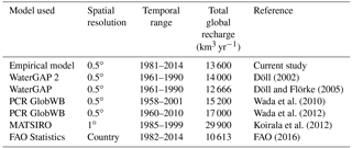
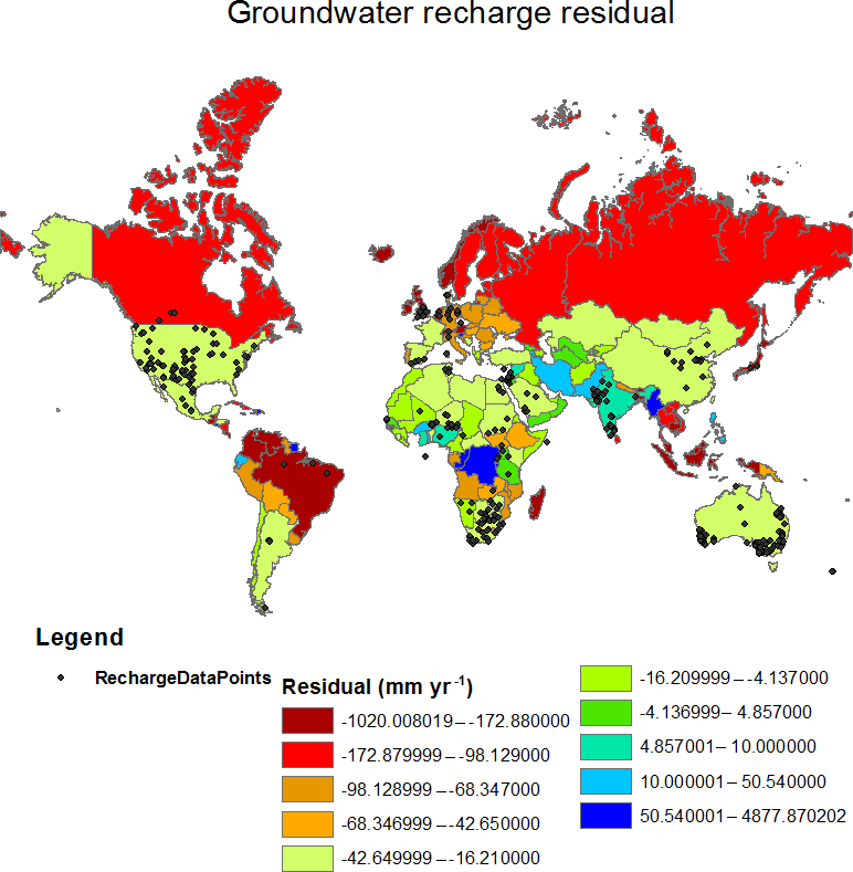
Figure 12 Spatial distribution of groundwater recharge residual (FAO estimates less model estimates) along with recharge sites selected for model building.

The total recharge estimated in this study is strongly consistent with results from complex global hydrological models. Long-term average annual recharge was found to be 134 mm yr⁻¹. The total recharge estimated in this study (13 600 km³ yr⁻¹) was very close to existing estimates of complex hydrological models except those using MATSIRO, which overestimates recharge in humid regions (Koirala et al., 2012). The results shown in Table 4 indicate that, compared to existing techniques, the model developed in this study can make recharge assessments with the same reliability but with fewer computational requirements. Moreover, the error in recharge prediction in this study was low, ranging from only −8 to 10 mm yr⁻¹ for 97.2 % of cases.

The global recharge map developed showed a similar pattern to recharge maps produced using complex global hydrological models. The results of this study indicate that recharge across the globe varied considerably as a function of spatial region, and was analogous to global distribution of climate zones (Scanlon et al., 2002). Humid regions had very high recharge compared to arid (semi-arid) regions, which is obviously due to the higher availability of water for recharge. Recharge was also affected by climate variability and climate extremes at a regional level (Scanlon et al., 2006; Wada et al., 2012). However, an effect of climate variability on inter-annual recharge at a global scale was not pronounced in our results. The potential reason for this is that the El Niño Southern Oscillation (ENSO), the primary factor determining climate variability globally, has converse effects in different parts of the world. The effects of increased precipitation in some parts of the world would have been counteracted by reductions in precipitation in other areas resulting in relatively small effects on inter-annual variation in global recharge.

5 Conclusion

This study presents a new method for identifying the major factors influencing groundwater recharge and using them to model large-scale groundwater recharge. The model was developed using a dataset compiled from the literature and containing groundwater recharge data from 715 sites. In contrast to conventional water balance recharge estimation, a multimodel analysis technique was used to build the model. The model developed in this study is purely empirical and has fewer computational requirements than existing large-scale recharge modelling methods. The 0.5^∘ global recharge estimates presented here are unique and more reliable because of the extensive validation done at different scales. Moreover, inclusion of a range of meteorological, topographical, lithological and vegetation factors adds to the predictive power of the model. The results of this investigation show that meteorological and vegetation factors had the most predictive power for recharge. The high dependency of recharge on meteorological predictors make it more vulnerable to climate change. Although it is a computationally efficient modelling method, the approach used in this study has some limitations. Firstly it does not include direct anthropogenic effects on the groundwater system or recharge by natural or artificial means, suggesting scope for further future development. Secondly, the recharge dataset used in this study did not include data points from frozen regions. Therefore, Greenland and Antarctica were excluded from the final recharge map. However, the model developed in this study and the recharge maps produced will aid policy makers in predicting future scenarios with respect to global groundwater availability.