the Creative Commons Attribution 4.0 License.
the Creative Commons Attribution 4.0 License.
 | 25 Apr 2018
Soil hydraulic material properties and layered architecture from time-lapse GPR
Stefan Jaumann
Kurt Roth
Quantitative knowledge of the subsurface material distribution and its effective soil hydraulic material properties is essential to predict soil water movement. Ground-penetrating radar (GPR) is a noninvasive and nondestructive geophysical measurement method that is suitable to monitor hydraulic processes. Previous studies showed that the GPR signal from a fluctuating groundwater table is sensitive to the soil water characteristic and the hydraulic conductivity function. In this work, we show that the GPR signal originating from both the subsurface architecture and the fluctuating groundwater table is suitable to estimate the position of layers within the subsurface architecture together with the associated effective soil hydraulic material properties with inversion methods. To that end, we parameterize the subsurface architecture, solve the Richards equation, convert the resulting water content to relative permittivity with the complex refractive index model (CRIM), and solve Maxwell's equations numerically. In order to analyze the GPR signal, we implemented a new heuristic algorithm that detects relevant signals in the radargram (events) and extracts the corresponding signal travel time and amplitude. This algorithm is applied to simulated as well as measured radargrams and the detected events are associated automatically. Using events instead of the full wave regularizes the inversion focussing on the relevant measurement signal. For optimization, we use a global–local approach with preconditioning. Starting from an ensemble of initial parameter sets drawn with a Latin hypercube algorithm, we sequentially couple a simulated annealing algorithm with a Levenberg–Marquardt algorithm. The method is applied to synthetic as well as measured data from the ASSESS test site. We show that the method yields reasonable estimates for the position of the layers as well as for the soil hydraulic material properties by comparing the results to references derived from ground truth data as well as from time domain reflectometry (TDR).
- Article
(4946 KB) - Full-text XML
- BibTeX
- EndNote


Quantitative understanding of soil water movement is in particular based on accurate knowledge of the subsurface architecture and the hydraulic material properties. As direct measurements are time-consuming and near to impossible at larger scales, soil hydraulic material properties are typically determined with indirect identification methods, such as inversion (Hopmans et al., 2002; Vrugt et al., 2008). Time domain reflectometry Robinson et al. (TDR, e.g., 2003) is a standard method to acquire the required measurement data, because it is sensitive to hydraulic processes. Yet, being an invasive method, the TDR sensors disturb the soil texture of interest and typically require the maintenance of a local measurement station. Hence, it is difficult to apply the method at larger scales or to transfer the sensors to another field site. Ground-penetrating radar Daniels (GPR, e.g., 2004); Neal (GPR, e.g., 2004) is an established noninvasive method for subsurface characterization and has the potential to become a standard method for efficient, accurate, and precise determination soil hydraulic material properties.
Available research studies regarding the estimation of hydraulic properties from GPR measurements may be categorized according to the applied methods for the different components of the research study, such as the (i) GPR measurement procedure, (ii) experiment type, (iii) GPR simulation method, (iv) optimization method, and (v) evaluation method of the GPR signal.
Most of these studies either use on-ground, off-ground, or borehole GPR measurements. On-ground measurements Buchner et al. (e.g., 2012); Busch et al. (e.g., 2012); Léger et al. (e.g., 2015) offer the most flexible approach. They have the disadvantage, however, that the antenna characteristics are influenced by the coupling to the ground. Off-ground measurements Lambot et al. (e.g., 2009); Jadoon et al. (e.g., 2012); Jonard et al. (e.g., 2015) avoid these effects, but the measurements are influenced by surface roughness. Cross-borehole measurements allow for high-resolution tomography of the subsurface Ernst et al. (e.g., 2007); Looms et al. (e.g., 2008); Scholer et al. (e.g., 2011) but require boreholes which are destructive and expensive.
The applied experiment types range from infiltration, fluctuating groundwater table, to evaporation. Infiltration experiments Léger et al. (e.g., 2014); Thoma et al. (e.g., 2014); Rossi et al. (e.g., 2015) are fast (hours) and provide indirect information about the near-surface material properties. Through its dependence on the form of the infiltration front or plume, the resulting GPR signal can get rather complicated to reproduce when used for quantitative evaluation. Difficulties arise from multiple reflections in the plume, waveguides in the infiltration front, and from noise originating for small-scale heterogeneity or fingering. In particular, if the infiltration is done artificially, accurate knowledge of the spatial distribution of the infiltration flux is required. Also simultaneous GPR measurements during the infiltration process are difficult, because the antenna coupling to the subsurface is influenced by the changing water content close to the surface. Fluctuating groundwater table experiments Bradford et al. (e.g., 2014); Léger et al. (e.g., 2015) require intermediate timescales (hours to days) and provide information about the material properties close to the groundwater table. These experiments are typically limited to fluvial or coastal areas or are induced artificially in test sites. Evaporation experiments Moghadas et al. (e.g., 2014) demand long timescales (weeks), because the hydraulic dynamics are slow at low water contents. Yet, this kind of experiment is important to understand the coupling of the pedosphere with the atmosphere.
The applied models to simulate the GPR signal are faced by an inherent tradeoff between performance and accuracy. Ray tracing (Léger et al., 2014, 2015) is fast but merely yields an approximate solution of Maxwell's equations. These equations can be solved analytically with Green's function Lambot et al. (e.g., 2009); Busch et al. (e.g., 2012); Jonard et al. (e.g., 2015) assuming a layered subsurface architecture. Alternatively, Maxwell's equations can be solved numerically with the finite differences time domain (FDTD) method Taflove and Hagness (e.g., 2000). This method is computationally expensive, but grants full flexibility concerning the source wavelet and the subsurface architecture Lampe et al. (e.g., 2003); Giannopoulos (e.g., 2005); Buchner et al. (e.g., 2012).
Due to the inherent oscillating nature of the electromagnetic signal, inversion of GPR data generally demands globally convergent and robust optimization techniques. Sequentially coupling a globally convergent search algorithm, e.g., the global multilevel coordinate search algorithm Huyer and Neumaier (GMCS, 1999) with the gradient-free locally convergent Nelder–Mead simplex algorithm Nelder and Mead (NMS, 1965), was successfully applied to estimate hydraulic material properties from GPR measurements Lambot et al. (e.g., 2004); Busch et al. (e.g., 2012); Moghadas et al. (e.g., 2014). The NMS was further developed to the shuffled complex evolution Duan et al. (SCE-UA, 1992) which has become a standard tool in hydrology and was also applied on GPR measurements Jadoon et al. (e.g., 2012); Léger et al. (e.g., 2014, 2015). Additionally, Markov chain Monte Carlo (MCMC) methods Scholer et al. (e.g., 2011); Thoma et al. (e.g., 2014); Jonard et al. (e.g., 2015) and data assimilation approaches Tran et al. (e.g., 2014); Manoli et al. (e.g., 2015); Rossi et al. (e.g., 2015) have been successfully applied so far.
The GPR signal has to be processed automatically for parameter estimation. Many full waveform inversion approaches directly use the resulting Green's function (e.g., Lambot et al., 2009; Busch et al., 2012; Jadoon et al., 2012) in the cost function. Using the full antenna signal may lead to many local minima prohibiting a reliable identification of the global minimum Bradford et al. (e.g., 2014). In contrast, filtering the radargram with convolution approaches to determine travel time and amplitude of a limited number of events leads to better convergence and may even allow the application of efficient locally convergent algorithms Buchner et al. (e.g., 2012).
In homogeneous materials, the transition zone above the groundwater table exhibits a smooth variation of the relative permittivity. Since the resulting GPR reflection is a superposition of a series of infinitesimal contributions along the transition zone, the detailed form of this reflection is sensitive to the variation of the relative permittivity. For simplicity, we refer to this reflection as transition zone reflection. Dagenbach et al. (2013) showed that this reflection is sensitive to the hydraulic material parameterization model. Bradford et al. (2014) measured the transition zone reflection of a drainage pumping test in a fluvial area with an antenna center frequency of 200 MHz and estimated hydraulic material properties. Klenk et al. (2015) employed numerical forward simulations and experiments using GPR antennas with higher antenna center frequency (400 and 600 MHz) for a more-detailed explanation of the transition zone reflection during imbibition, equilibration, and drainage. They also concluded that the transition zone reflection is sensitive to hydraulic material properties.
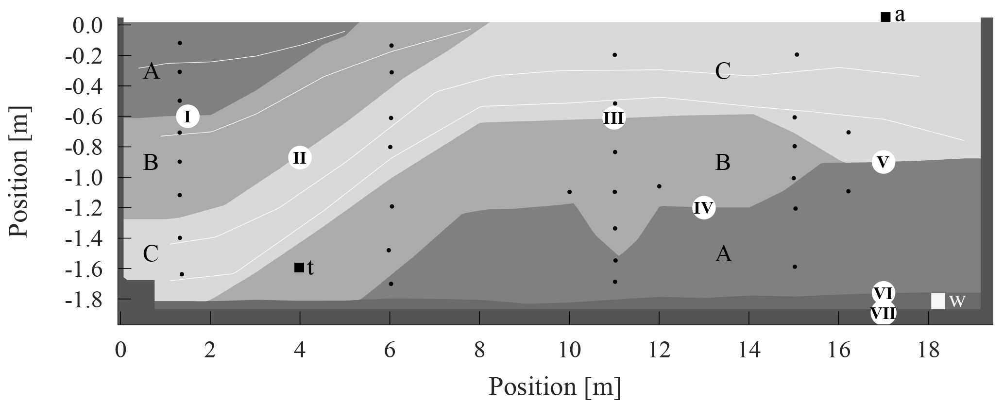
Figure 1ASSESS provides an effectively 2-D subsurface architecture consisting of three kinds of sand (A, B, and C). During the experiment that is evaluated in this work, the groundwater table was manipulated via a groundwater well (white square at 18.3 m). The resulting hydraulic dynamics were monitored automatically with a stationary GPR antenna (black square at 17.05 m), a tensiometer (black square, at 4.0 m), and 32 TDR sensors (black dots). A gravel layer below the sands allows for a rapid water pressure distribution at the lower boundary of the site. An L-element (left wall, at 0.4 m) and compaction interfaces (white lines) result from the construction of the site. Additionally to those visualized, GPR evidence indicates additional compaction interfaces (Fig. 14) that were not determined during construction. Roman numerals (I)–(VII) indicate material interfaces referred to in the text. Note the different scales on the horizontal and vertical axes.
This work builds upon previously published methods for simultaneous estimation of the subsurface architecture and the effective water content based on on-ground multi-offset GPR measurement data Gerhards et al. (e.g., 2008); Buchner et al. (e.g., 2012). In order to develop methods to additionally estimate hydraulic material properties, the ASSESS test site was forced with a fluctuating groundwater table ensuring large hydraulic dynamics. In this work, we use the resulting transition zone reflection together with reflections originating from material interfaces to estimate the positions of layers within the subsurface architecture as well as their hydraulic material properties. Running 2-D or even 3-D measurements and inversions is a massive experimental and computational effort. Prior to embarking on this, the individual steps must be demonstrated. To this end, the experiment was monitored with a stationary on-ground bistatic antenna that operates at a center frequency of 400 MHz, leading to time-lapse GPR measurement data. The hydraulic dynamics below this antenna are modeled in 1-D using the Richards equation. The resulting water content distribution is extruded and converted to a relative permittivity distribution to solve Maxwell's equations in 2-D. Similar to Buchner et al. (2012), we developed a new heuristic semiautomatic approach to extract the signal travel time and amplitude of relevant reflections in the radargram (events). This approach is applied to both the simulated and measured radargram and the corresponding events are associated automatically. For optimization, a global–local inversion approach with preconditioning is applied. To that end, we draw parameter sets with a Latin hypercube algorithm that serve as initial parameters for the preconditioning step. In this step, a simulated annealing algorithm and a Levenberg–Marquardt algorithm are sequentially coupled using a subsampled data set for a limited number of iterations. Subsequently, the resulting parameters of the preconditioning step serve as initial parameters for another run of the Levenberg–Marquardt algorithm using the full data set. We show that this procedure accurately estimates the layered subsurface architecture as well as the associated effective hydraulic material properties for synthetic and measurement data.
2.1 ASSESS
The measurement data for this work are acquired at an approximately large the test site (ASSESS) which is located near Heidelberg, Germany, and provides an effectively 2-D subsurface architecture consisting of three kinds of sands (Fig. 1). Below the sands, an approximately 0.1 m thick gravel layer ensures rapid distribution of the water pressure at the lower boundary. This gravel layer is separated from the sand via a geotextile and is the only connection of the site to a groundwater well. The groundwater well is in particular used to manipulate the groundwater table by pumping water in and out of the well. The groundwater table in the test site is automatically determined with a tensiometer (UMS T4-191). The test site incorporates 32 soil temperature and TDR sensors which are operated via a weather station and a Campbell Scientific TDR100. The site is confined by a basement layer below the gravel layer and by a wall at each of the four sides. During the construction, the materials were compacted with a vibrating plate for stabilization.
2.2 Representation
Quantitative understanding of a system of interest requires its mathematical representation. Based on Bauser et al. (2016), we define the representation of a system as a set consisting of (i) the dynamics corresponding to the mathematical propagation of the variable of interest at predefined scales in space and time, (ii) the coupling to the sub-scale physics through typically heuristic material properties, (iii) the coupling to the super-scale physics through the forcing in space and time, and (iv) the state corresponding to the variable of interest that is propagated by the dynamics.
2.2.1 Dynamics
The standard model to describe the volumetric water content θ (–) and the matric head hm (m) in space and time t (s) is the Richards equation (Richards, 1931),
To solve this partial differential equation, the soil water characteristic θ(hm) and the hydraulic conductivity function Kw(θ) are required. The direction of gravity is indicated with the unit vector in z direction ez.
2.2.2 Sub-scale physics
We choose the Brooks–Corey parameterization (Brooks and Corey, 1966) for the soil water characteristic θ(hm), since it describes the materials in ASSESS appropriately (Dagenbach et al., 2013). Inverting this parameterization for leads to
with a saturated water content θs (–), a residual water content θr (–), a scaling parameter h0 (m) related to the air entry pressure (h0<0 m), and a shape parameter λ (–) related to the pore size distribution (λ>0).
The hydraulic conductivity function Kw(θ) is parameterized combining the Brooks–Corey parameterization with the hydraulic conductivity model of Mualem (1976). This yields
with the saturated hydraulic conductivity Ks (m s−1) and a tortuosity factor τ (–).
2.2.3 Forcing
In order to provide the measurement data for this study, ASSESS was forced with a fluctuating groundwater table leading to two characteristic phases comprising an initial drainage phase and a multistep imbibition phase (Fig. 2). The experiment was realized at the end of November and the weather was cloudy with 2–7 ∘C air temperature. Hence, evaporation is neglected in this work. Further details about the experiment are given by Jaumann and Roth (2017).
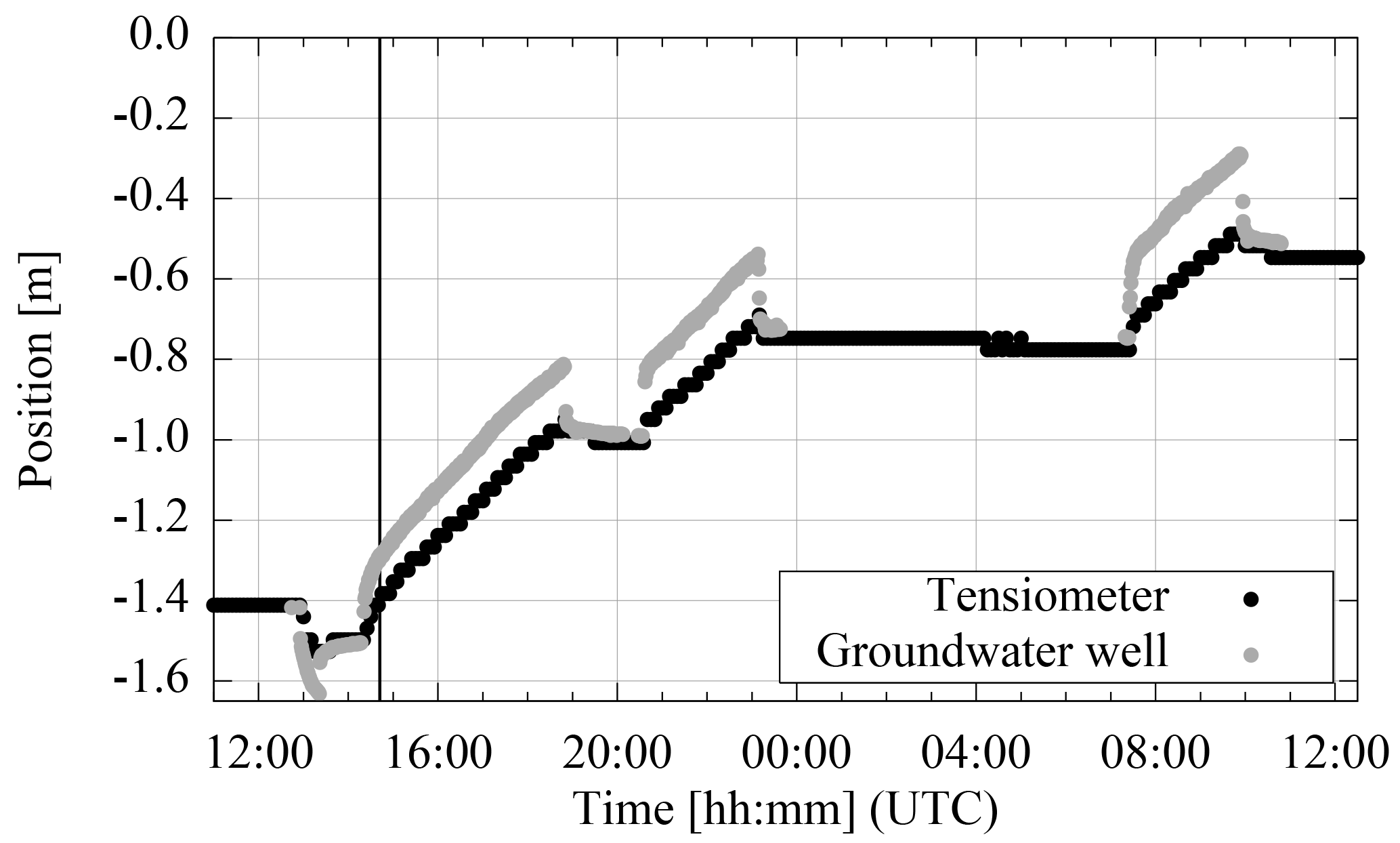
Figure 2During the experiment with two distinct phases (initial drainage and multistep imbibition – separated by the vertical line), the position of the groundwater table was measured manually in the groundwater well and automatically with the tensiometer (Fig. 1). The difference between them is proportional to the driving force of water flow in the gravel layer.
2.2.4 State
During the experiment, the groundwater table was measured (i) automatically with a tensiometer and (ii) manually via the groundwater well (Fig. 2). The hydraulic state was monitored with a stationary GPR antenna (Fig. 1). This shielded bistatic single-offset 400 MHz GPR antenna (Ingegneria dei Sistemi S.p.A., Italy) has an internal antenna separation of 0.14 m. The measurement resolution was set to 2048 samples for 60 ns. The acquired GPR data are analyzed in detail in Sect. 3.3. Additionally, a mean soil temperature () and a mean electrical conductivity () was estimated from TDR-related measurements available in ASSESS. The electrical conductivity was evaluated from the TDR pulse shape and thus includes the direct current conductivity as well as dielectric losses. For this evaluation and the corresponding temperature correction, we implemented the methods of Heimovaara et al. (1995).
The observation operator required to compare the simulated hydraulic state with the GPR measurement data involves the solution of the time-dependent Maxwell equations in linear macroscopic isotropic media. These equations quantify the propagation of the electric field E and the magnetic field B (Jackson, 1999):
The dielectric permittivity ε=ε0εr, magnetic permeability μ=μ0μr, and electrical conductivity σ are generally spatially variable and represent the electromagnetic properties of the subsurface. Here, we use the static relative permittivity , neglect dispersive effects (), and assume the permittivity to be real valued (εr∈ℝ). The relative magnetic permeability is assumed to be that of vacuum (μr=1). The source current density J is applied at the position of the transmitter antenna.
The relative permittivity of the subsurface is calculated from the water content distribution using the complex refractive index model (CRIM, Birchak et al., 1974):
The application of the CRIM requires knowledge of the porosity ϕ, the relative permittivity of water εr,w, the relative permittivity of air εr,a, and the relative permittivity of the soil matrix εr,s. The relative permittivity of air εr,a was set to 1. Since we assume that the soil matrix consists mainly of quartz (SiO2) grains, the relative permittivity of the soil matrix εr,s was set to 5 (Carmichael, 1989). We further assume that porosity ϕ is equal to the saturated water content θs (Eq. 2). The dependency of the static relative permittivity of water εr,w on the soil temperature Ts (∘C) is parameterized following Kaatze (1989)
The electrical conductivity σ of the subsurface is assumed to be constant in space and time. As for the relative permittivity, we neglect dispersive effects of the electrical conductivity () and assume it to be real valued (σ∈ℝ).
2.3 GPR analysis
To analyze the GPR data, we follow Buchner et al. (2012) and extract the travel time t and the corresponding amplitude A for M samples of the GPR signal (events)
with a heuristic approach, because this allows us to focus on the phenomena that are represented in the model. However, to associate the events extracted from the measured signal with events extracted from the simulated signal, this procedure demands an automatic event association algorithm. Thus, the evaluation method consist of four steps: (i) signal processing, (ii) event detection, (iii) event selection, and (iv) event association (Fig. 3).
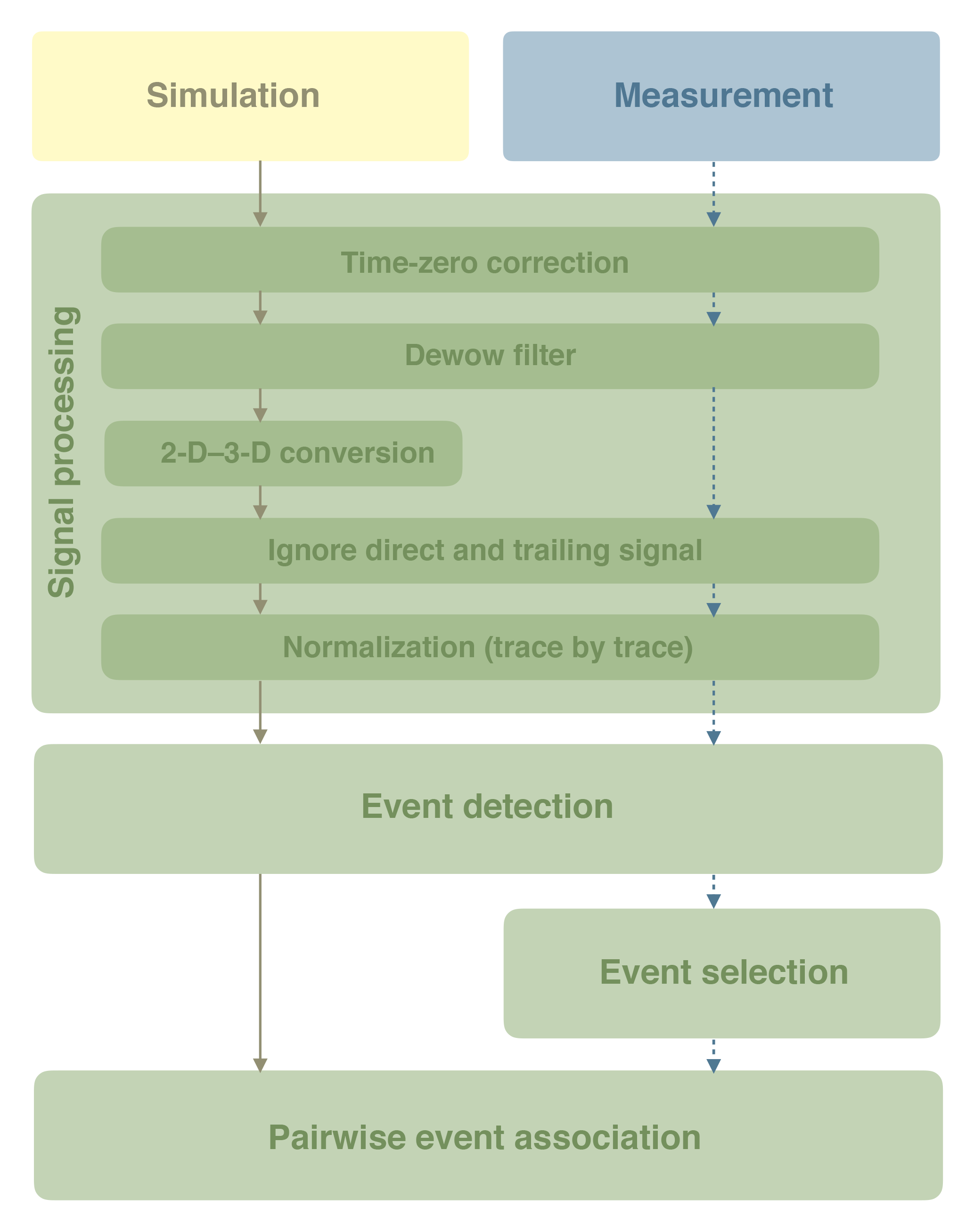
Figure 3The GPR data evaluation method presented in this section consists of four main steps. In the first step, the signal is processed (Sect. 2.3.1). The 2-D to 3-D conversion in this step is applied to the simulated data. In the second step, extrema in the GPR signal are detected (Sect. 2.3.2). The detected events in the measurement data can be selected manually for the subsequent evaluation (Sect. 2.3.3). This ensures that the optimization focuses only on the most relevant information in the data. Finally, the most plausible association of simulated and measured events is determined (Sect. 2.3.4). Note that for each parameter set that is tested during the optimization procedure, the simulation data are evaluated automatically (solid lines). In contrast, the measurement data are only evaluated once before starting the optimization procedure (dashed lines).
2.3.1 Signal processing
The processing of the GPR signal includes the following step: (i) time-zero correction, (ii) dewow filter, (iii) 2-D to 3-D conversion, (iv) removal of the direct signal (particularly including the direct wave and the ground wave) and the trailing signal (signal at the end of the trace which is disturbed by the dewow filter), and (v) normalization (Fig. 3).
Since the time-zero of the GPR antennas changes over time, we pick the direct signal and subtract the evaluated travel time from each trace of the radargram for time-zero correction. Subsequently, a dewow filter is applied to subtract inherent low-frequency wow noise of the GPR signal. Because the observation is in 3-D and the simulation in 2-D, we convert the simulated signal to 2.5-D, meaning to 3-D with translational symmetry perpendicular to the survey line and parallel to the ground surface (Bleistein, 1986). The ASSESS site conforms to this 2-D requirement (Sect. 2.1). For the conversion, each trace is transformed to the frequency domain with the fast Fourier transform (FFT, denoted by ). Afterwards, the electric field is modified depending on the angular frequency ω:
where i is the complex unit, Ci is a constant (m), and σc denotes the integral of the velocity with respect to the length s of the ray trajectory. Assuming a direct ray path and a horizontal reflector with the reflector distance d as well as the mean square root of the dielectric permittivity along the ray path, this is leads to
Subsequently, all traces are transformed back to the time domain with the inverse FFT. Due to the frequency conversion and the manipulation, a high-frequency noise remains on the signal which is smoothed with a fourth-order Savitzky–Golay filter (e.g., Press, 2007, we employed the implementation of the “signal” package for GNU Octave: https://octave.sourceforge.io/signal/) using a window width of 41 samples. Subsequently, the direct signal and the trailing signal of the dewow filter are set to zero. Finally, each trace is normalized to its maximal absolute amplitude since the absolute power of the GPR source is typically unknown. Thus, the value of the constant Ci in Eq. (6) also becomes irrelevant.
2.3.2 Event detection
In this step, events are detected in each trace separately (Fig. 4). To facilitate the detection of relevant events at large signal travel times, the amplitude of the processed signal (Sect. 2.3.1) is amplified quadratically with travel time using an arbitrary gain function that was shown to work well. Subsequently, the extrema of the amplified amplitude are detected with a local neighborhood search. We keep a predefined number of events (15) with the largest amplified absolute amplitude. If the non-amplified amplitude of a detected extremum is below a predefined amplitude threshold (0.006), the event is discarded in any case. In order to correct the perturbation in travel time due to the amplification and to cope with the discrete measurement resolution, we fit a Gaussian curve centered at the travel time of the detected event with a width of ±5 samples to the non-amplified amplitude of the processed signal. The travel time of the resulting extremum of the Gaussian fit is directly used for the following evaluation. The amplitude of the extremum is used as the amplitude of this event. This procedure makes the form of the previously applied gain function irrelevant. The amplitude of all detected events is normalized with the absolute maximal amplitude of all detected events within the same trace.
2.3.3 Event selection
After the event detection, the measured signal and the detected events (Sect. 2.3.2) are inspected manually. In this one-time processing step, events can either be deleted or added manually. Thus, it can be ensured, that only those events that are also represented in the model enter the parameter estimation. This step is skipped for the analysis of the simulated data. The resulting amplitude of the selected events is normalized with the absolute maximal amplitude of all selected events of each trace.

Figure 4The detected events of the first trace of the synthetic radargram analyzed in Sect. 3.2. The amplitude of a trace is searched for extrema with a neighborhood search algorithm. For the subsequent evaluation, the amplitude of the detected events is normalized to the maximal absolute amplitude of all events detected in the trace. The direct signal and the trailing signal of the dewow filter with normalized travel times <0.06 and >0.89, respectively, are set to zero in a processing step (Sect. 2.3.1) and possible events close to these signals are ignored.
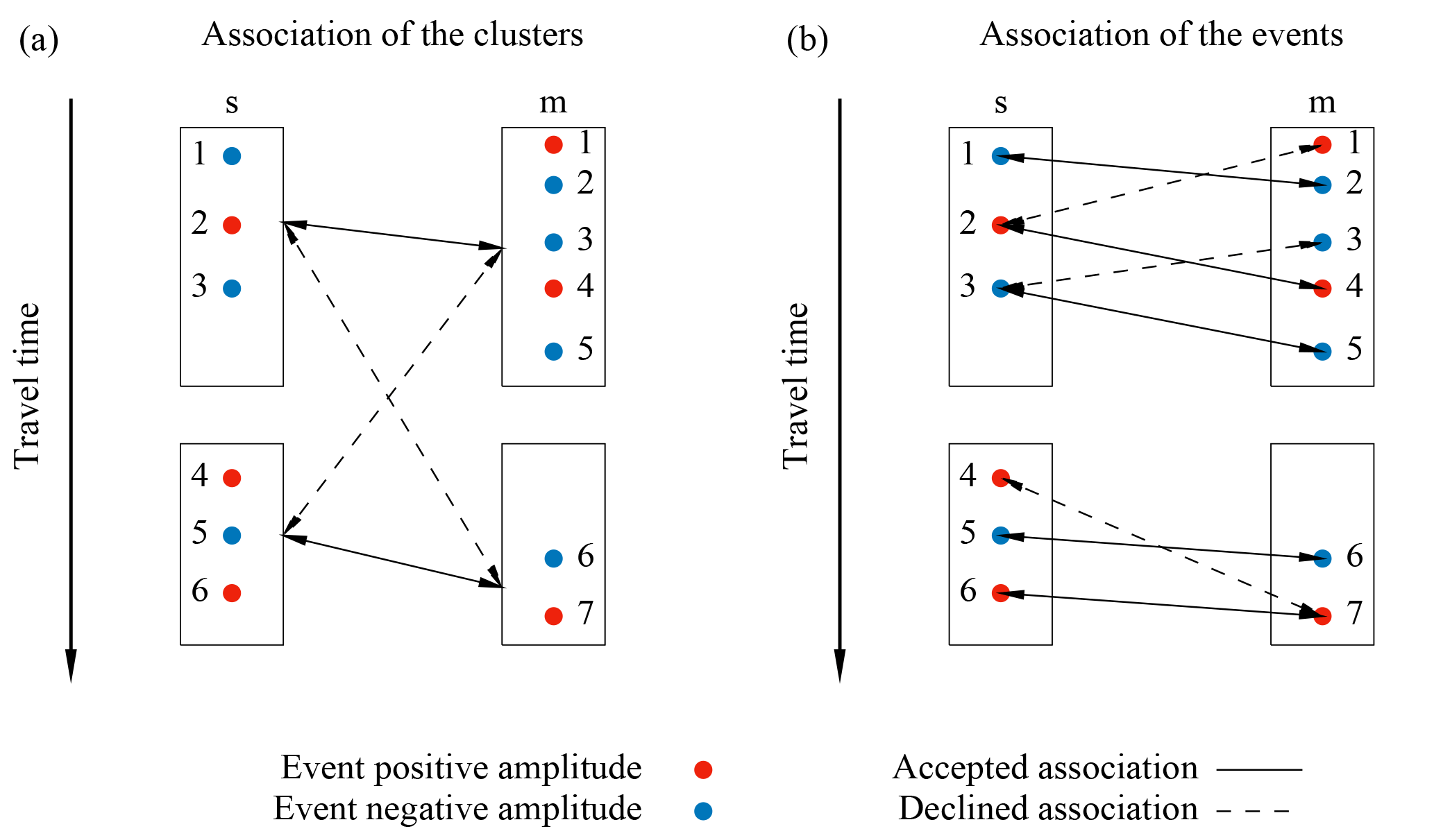
Figure 5Example of the association of simulated (s) and measured (m) events with indices 1–6 and 1–7, respectively. The color of the dots indicates the sign of amplitude of the events. (a) The detected events (Fig. 4) are aggregated in clusters to minimize the number of possible event combinations. The clusters are associated such that the summed absolute travel time difference of the mean travel time of the events in the cluster is minimal. (b) The events in the clusters are associated according to consistent temporal order and amplitude sign. Hence, if is associated with event , event cannot be associated with event , if or . Solid (dashed) arrows indicate some of the accepted (declined) association combinations. The combination with the maximal number of associations and minimal summed absolute travel time difference is used for evaluation. Thus, for example is associated with and not with .
2.3.4 Pairwise event association
The selected events extracted from the measured data have to be associated with the detected events extracted from the simulated data for the parameter estimation. To this end, Buchner et al. (2012) tested all possible combinations of events, using the one with the minimal summed absolute travel time difference. However, this is only feasible for a small number of events. As we are not using a Gaussian convolution of the data but the data themselves, the number of events increases. Hence, testing all combinations is often prohibitively expensive.
In order to exclude combinations a priori, the detected events are aggregated in clusters (Fig. 5a). Then, these clusters are associated by testing all possible combinations and finally using the combination with the minimal summed absolute travel time difference. Afterwards, those events that are aggregated in the associated clusters are associated themselves. The applied association procedure requires the events to have an identical amplitude sign and a consistent temporal order which reflects the principle of causality (Fig. 5b). After iterating over all allowed combinations, the association with the maximal number of associated events and the minimal summed absolute travel time difference is used. It is critical to also consider combinations where some intermediate events (e.g., in Fig. 5) cannot be associated.
After the association of the events, outliers are detected by calculating the mean and standard deviation of the travel time differences. All associations that exhibit an absolute travel time difference larger than 3 standard deviations of all absolute travel time differences are discarded. Finally, the amplitude of the associated events is normalized to the maximal absolute amplitude of the associated events of each trace separately for the simulation and the measurement.
2.4 Parameter estimation
Inversion of GPR data typically requires globally convergent parameter estimation algorithms which are computationally expensive. In order to keep the parameter estimation procedure efficient, we use an iterative strategy (Fig. 6). We start the optimization procedure by drawing an ensemble of initial parameter sets with a Latin hypercube algorithm (implemented by the pyDOE package, https://github.com/tisimst/pyDOE).
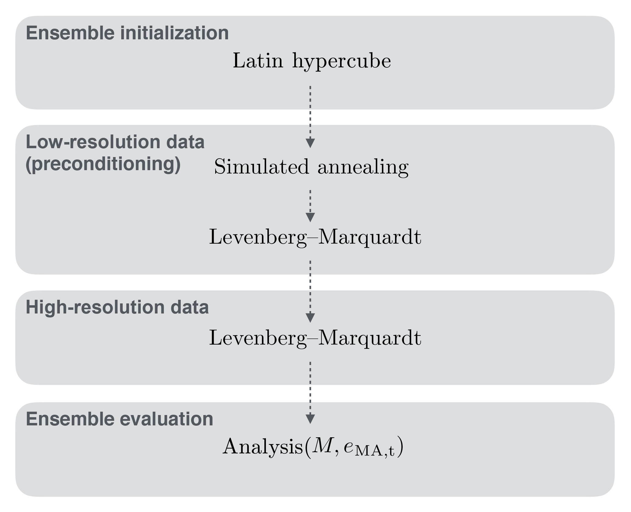
Figure 6We choose a sequentially coupled parameter estimation procedure which (i) allows minimizing the computational cost and (ii) facilitates the implementation of tagging (Sect. 2.4.1). Therefore, Latin-hypercube-sampled parameter sets are preconditioned with a data set with reduced number of traces (low-resolution data) by sequentially coupling the simulated annealing algorithm and the Levenberg–Marquardt algorithm. The preconditioned parameter sets for each ensemble member serve as initial parameters for the final parameter estimation based on high-resolution data. The subsequent evaluation of the ensemble is based on the number of associated events M and the mean absolute error in travel time eMA,t (Sect. 3.1.2).
The most expensive operation of the forward simulation is the calculation of the observation operator, which includes the solution of Maxwell's equations (Sect. 2.2.4) and the subsequent event association (Sect. 2.3). Since time-lapse GPR data are highly correlated in experiment time (e.g., Fig. 14b), we equidistantly subsample the number of traces of the time-lapse GPR radargram and generate a data set with lower temporal resolution. Those data are used to improve the distribution of the initial parameters (preconditioning). Therefore, the drawn parameter sets are used to initialize the simulated annealing algorithm (Sect. 2.4.2) which allows for a robust and fast parameter update. The resulting parameters then serve as initial parameters for the Levenberg–Marquardt algorithm (Sect. 2.4.3) which concludes the preconditioning step. The resulting parameters of the preconditioning step are used as the initial parameter sets for the more expensive optimization of high-resolution data set with the Levenberg–Marquardt algorithm. The details of the setup and the analysis of the parameter estimation are given in Sect. 3.1.2.
2.4.1 Cost function
Assuming P parameters pπ and M associations of measured events with simulated events , the cost function S(p) is given by
with the constant standard deviation of the measured normalized travel times and of the measured normalized amplitudes . This leads to the standardized residuals in travel time rt,μ and amplitude rA,μ.
Due to the oscillating nature of the GPR signal and due to the applied GPR data evaluation (Sect. 2.3), the cost function is not necessarily convex and may even be discontinuous at some points, because the number of associated events M may change during the minimization process. Hence, adding and removing associations of events requires a compensation to prevent the cost function from becoming discontinuous. To this end, Buchner et al. (2012) introduced tagging. If the number of measured events is smaller than the number of the simulated events, the simulated events that are not associated are excluded. Alternatively, if there are more measured events, measured events without a partner are tagged as partnerless. If a reflection event has been tagged and becomes untagged after the parameter update, the contribution of the event and its new partner to the cost function is added to the previous cost. If an event has not been tagged and becomes tagged after the parameter update, the contribution to the cost function is subtracted from the previous cost.
2.4.2 Simulated annealing
We choose the simulated annealing algorithm (Press, 2007) to start the minimization of the cost function (Eq. 8), because this algorithm is gradient-free and updates the parameters randomly. In addition, the implementation of tagging (Sect. 2.4.1), which can be implemented easily for this algorithm, no further regularization is required due to its random parameter update. Hence, this algorithm is in particular suitable for initial iterations where the association of the single events may lead to an inconsistent association of the reflections. Once the reflections are associated consistently, the Levenberg–Marquardt algorithm is typically more efficient than the simulated annealing algorithm.
If the parameter update is drawn from the whole parameter space, the simulated annealing algorithm is globally convergent. However, this approach is typically inefficient. Hence, we search the neighborhood for better parameters starting from the Latin-hypercube-sampled initial parameters pπ,0. For each iteration i , new parameters are proposed randomly via
with a mobility parameter m=0.1, uniformly distributed random number , and the parameter limits pπ,max and pπ,min. In order provide the control parameter T, which is an analog of temperature, we choose an exponential cooling schedule
with α=0.85 and initial temperature T0=103 which is of the order of the initial cost. According to Metropolis et al. (1953), we draw an uniformly distributed random number ; calculate the acceptance probability
choosing parameter k=1; and accept the proposed parameter set if or else draw a new parameter set.
2.4.3 Levenberg–Marquardt
The Levenberg–Marquardt algorithm is implemented as described by Jaumann and Roth (2017). The application of this gradient-based algorithm on GPR data requires the implementation of tagging (Sect. 2.4.1) as well as additional regularization of the optimization. This regularization can be achieved by focussing in particular on the improvement of the small residuals, because if the small residuals improve, the larger residuals are likely to also improve in subsequent iterations due to the temporal correlation of the time-lapse data. Therefore, events with or are tagged. Tagged events are excluded from the optimization by setting those entries in the Jacobian matrix () to zero. The event association may also change during the perturbation of the parameters for the numerical assembly of the Jacobian matrix. This can lead to large changes in the residuals, which in turn may lead to a disturbed parameter update. Hence, corresponding entries of large changes in the residual are also set to zero together with entries of the Jacobian matrix that are larger than 104.
We choose λLM,initial=5 as the initial value for λLM and apply the delayed gratification method by decreasing (increasing) λLM by a factor of 2 (3) if the parameter update is successful (not successful). This ensures that the algorithm takes small steps such that the association and the Jacobian matrix can adapt smoothly.
In this section, the methods presented in the previous section are applied to GPR data. First, the setup of the case study, its implementation and the detailed setup of the parameter estimation procedure are explained (Sect. 3.1). Subsequently, the suitability of the presented methods to estimate the subsurface architecture and the corresponding soil hydraulic material properties is first tested with synthetic data (Sect. 3.2). Finally, the methods are applied to measurement data (Sect. 3.3).
3.1 Setup of the case study
3.1.1 Implementation
In this work, the subsurface architecture of ASSESS is represented with layers. The position of these layers is parameterized and can be estimated. For illustration, the setup is shown in Fig. 7. The Richards equation (Eq. 1) is solved numerically with μφ (muPhi, Ippisch et al., 2006), which uses a cell-centered finite volume scheme with full upwinding in space and an implicit Euler scheme in time. The nonlinear equations are linearized by an inexact Newton method with line search and the linear equations are solved with an algebraic multigrid solver. We solve the Richards equation in 1-D (z dimension) on a structured grid with a resolution of ≈0.005 m. The simulated water content is converted to relative permittivity via the CRIM using the mean soil temperature (Sect. 2.2.4). Since Maxwell's equations are solved in 2-D, the simulated 1-D permittivity distribution is extruded in the y dimension using the same spatial resolution. The total size of the represented subsurface architecture is 1.0 m×1.9 m. Generally, the boundary condition is implemented with a Neumann no-flow condition. However, during the forcing phases, we prescribe the measured groundwater table as a Dirichlet boundary condition at the position of the groundwater well. We initialize the simulation with hydraulic equilibrium based on the measured groundwater table position.
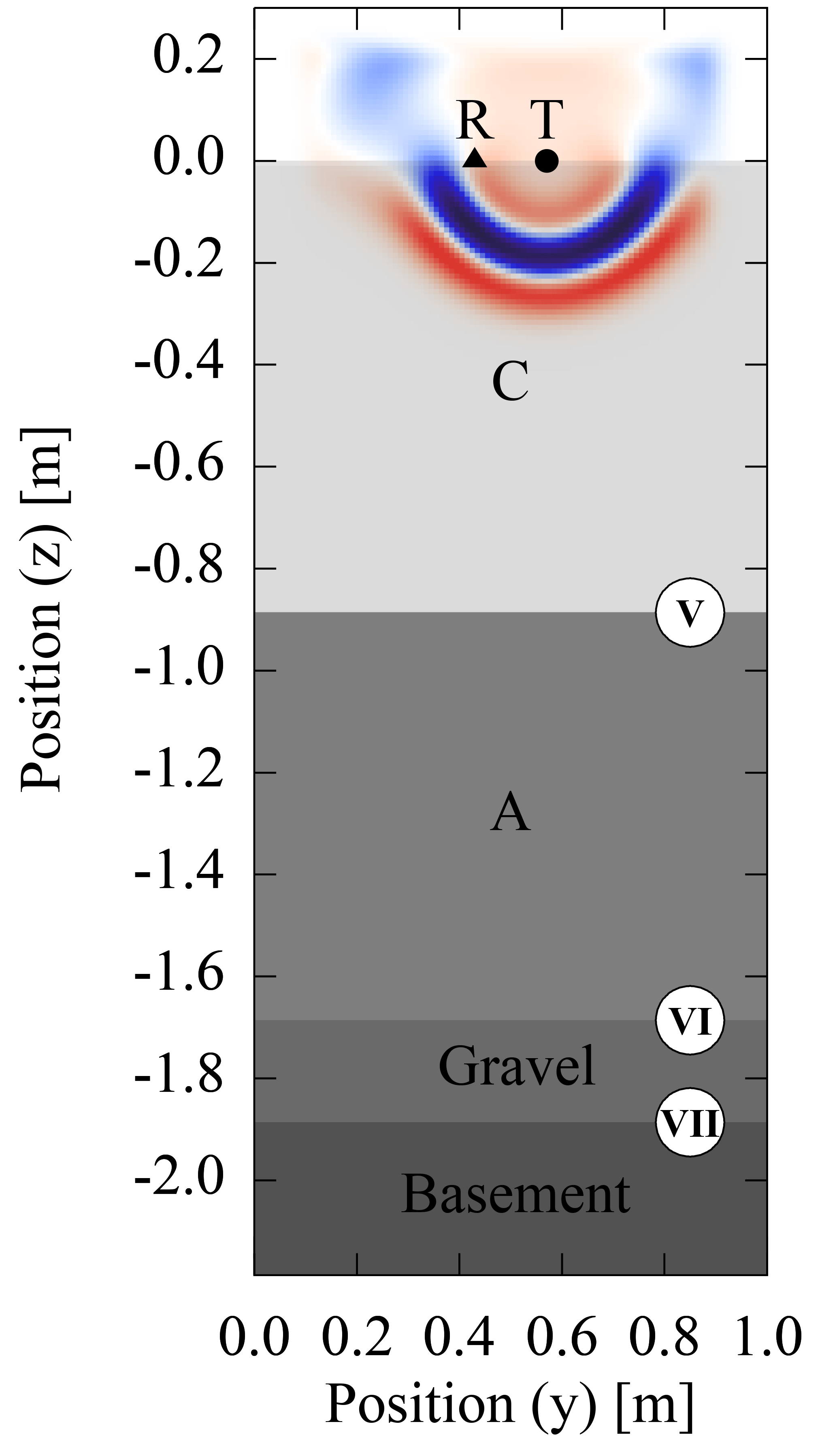
Figure 7For the simulation of the GPR signal, we assume a layered subsurface architecture (Fig. 1). The transmitter of the antenna is represented with an infinitesimal dipole (T) and the electric field is read at the position of the receiver antenna (R). A perfectly matched layer is used as boundary condition. The x component of the resulting electric field after 5 ns is shown. The markers for the material interfaces are used consistently in this work. The position of the interface of materials C and A (V) as well the position of the interface of materials A and gravel (VI) are parameterized (dV and dVI) and can be estimated.
To simulate the temporal propagation of the electromagnetic signal, we solve Maxwell's equations (Sect. 2.2.4) in 2-D with the MIT electromagnetic equation propagation software Oskooi et al. (MEEP, 2010). The transmitter antenna is represented with an infinite dipole pointing in x dimension (Fig. 7). Thus, we neglect any effects from the real antenna geometry (bow tie), cross coupling, or antenna shielding. The antenna source current density J is given by the first derivative of a Gaussian-shaped excitation function leading to a Ricker wavelet with a center frequency of 400 MHz. The receiver antenna is not represented explicitly. Instead, Ex is read directly at the position of the receiver antenna. We use the antenna separation of the real GPR system (0.14 m) in the simulation. Perfectly matched layers of 0.15 m thickness serve as boundary condition. The electromagnetic fields in the domain are zero initially.
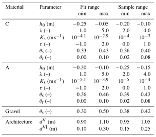
Table 1The fit range limits the parameter space available for parameter estimation and is in particular used by the simulated annealing algorithm to draw parameter updates (Sect. 2.4.2). The sample range is used to generate an ensemble of initial parameter sets with a Latin hypercube algorithm.
We use one-tenth of the minimal wavelength λw,min as the upper limit for the spatial resolution Δz:
with the speed of light in vacuum c0, maximal frequency , and corresponding to . Hence, we choose the numerical resolution Δz=0.005 m for the 2-D isotropic, structured, and rectangular grid. The Courant number for the FDTD method is set to 0.5.
To avoid multiple reflections at the air–soil boundary, we set the relative permittivity above the soil to 3.5, which is typical for dry sand. This is justified, because the air wave and the ground wave are not evaluated and the amplitude of the detected events is normalized. The permittivity of the basement below ASSESS is set to 23.0 based on previous simulations. The electrical conductivity of the subsurface σ is set to 0.003 S m−1 (Sect. 2.2.4). All electromagnetic properties are smoothed by MEEP according to Farjadpour et al. (2006).
The GPR data are evaluated according to Sect. 2.3. The detection of the clusters is chosen to be identical for the simulated and the measured data. The characteristic shape of the time-lapse radargram allows separating the clusters at a specific normalized travel time (tsplit=0.5) for all traces. Hence, all events with a travel time t≤tsplit are in cluster 1 and the others are in cluster 2.
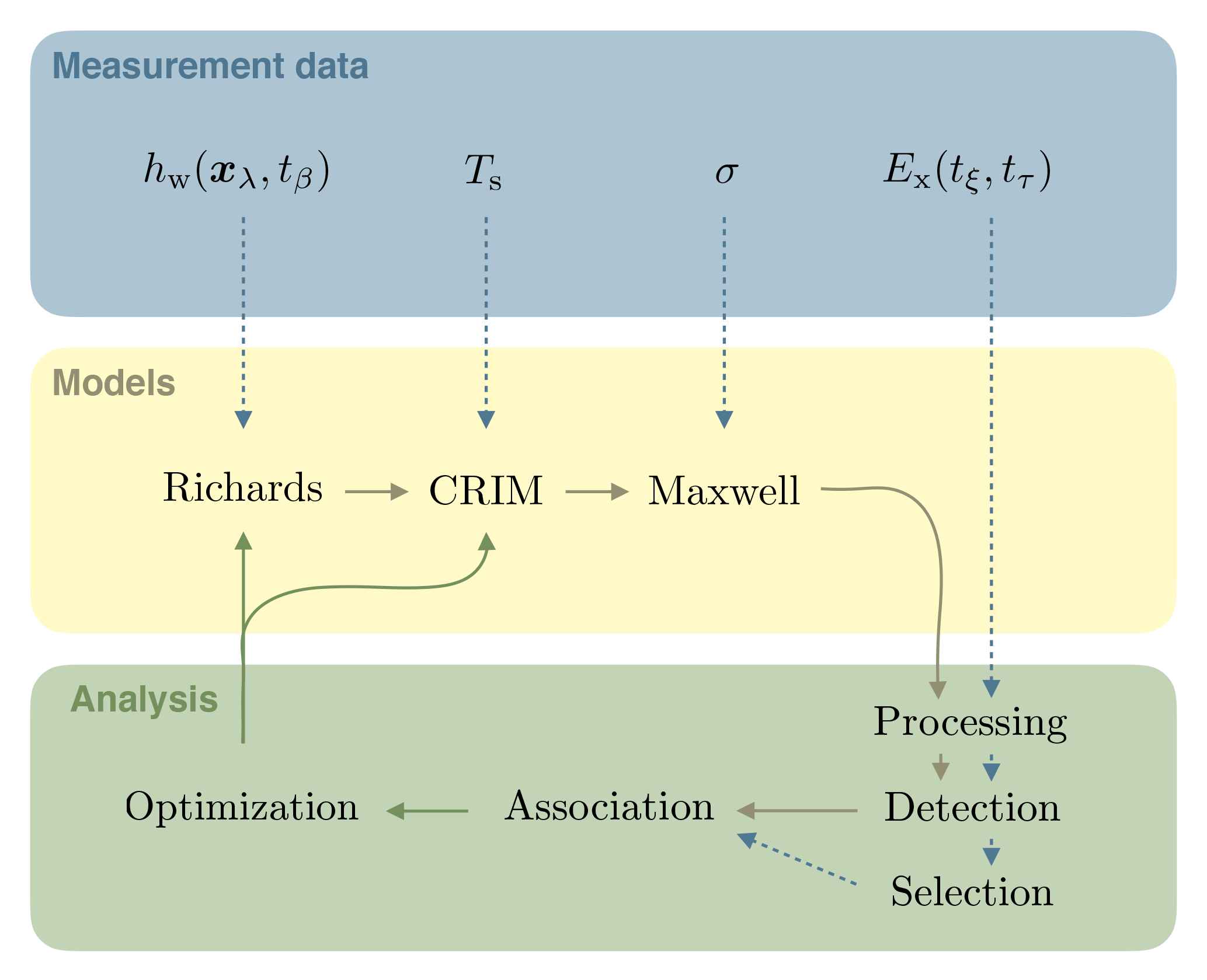
Figure 8The general setup of the optimization is sketched with this figure. The available hydraulic potential hwt is measured at the position of the groundwater well xλ times tβ. These measurements are used as a boundary condition for the Richards equation (Sect. 2.2.1). Estimates for the soil temperature Ts and the electrical conductivity σ are derived from TDR-related measurements. The actual signal of the GPR system is proportional to the x component of the electric field Ex and measured discretely at experiment time tξ and signal travel time tτ. This signal is processed (Sect. 2.3.1) and used for event detection (Sect. 2.3.2). Based on the detected events in the measurement data, other events can be either added or deleted in the subsequent event selection step (Sect. 2.3.3). The simulated water content distribution is converted to relative permittivity distribution with the CRIM and used to solve Maxwell's equations (Sects. 2.2.4 and 3.1.1). After the processing step and the event detection, the simulated events are assigned to measured events (Sect. 2.3.4). The resulting mapping of the events is used to calculate the cost in the optimization step (Sect. 2.4). Dashed arrows indicate initial processing steps, whereas solid arrows indicate iterative steps required for the optimization.
3.1.2 Setup of the parameter estimation
The general setup of the optimization is explained with Fig. 8. This setup is used in a sequential approach (Fig. 6) with a preconditioning step for which we subsampled the number of the traces of the time-lapse GPR data to generate a data set with decreased temporal resolution. The data set with high (low) resolution includes 86 (9) traces corresponding to one trace per 15 (150) min. Hence, both data sets subsample the actually measured number of traces (one trace per ≈30 s) equidistantly in time. Within the sample range given in Table 1, 60 initial parameter sets are drawn with the Latin hypercube algorithm and the data set with low temporal resolution is used to improve these parameter sets running 200 iterations of the simulated annealing algorithm. The parameter fit range given in Table 1 determines the parameter update via pπ,max and pπ,max according to Eq. (8). After the application of the simulated annealing algorithm, maximally 15 iterations of the Levenberg–Marquardt algorithm are run. This optimization completes the preconditioning step. The resulting parameter sets serve as initial parameters for the Levenberg–Marquardt algorithm which is applied to the data with high temporal resolution.
In order to evaluate the performance of the ensemble members, the mean absolute error in normalized travel time eMA,ta is used since this statistical measure is independent of the number of associated events. The number of associated events is accounted for by evaluating only those 10 members with minimal eMA,t that associated at least 85 % of the measured events. Each of these members has locally optimal parameters. However, the exact position of these local minima typically depends on the initial parameters and the random numbers drawn in the simulated annealing algorithm. There is also no guarantee that the global optimum was found by one of the ensemble members. However, the distribution of these 10 best ensemble members contains valuable information about the shape of the cost function. To account for this information, we (i) analyze the mean parameter set of the best members and (ii) use the standard deviation to indicate the uncertainty of these parameters. Notice that the mean parameter set is not necessarily optimal. However, if uncertainty of the resulting parameters is small, the mean parameter set is typically more reliable than the parameter set of the best ensemble member.
The standard deviations of the measured data, and for normalized travel times and amplitudes, respectively, are used to standardize the residuals of the cost function (Eq. 8). These standard deviations were calculated from travel time and amplitude data acquired by picking different reflections with approximately constant travel time. In order to perturb the travel time and amplitude of the selected events of the synthetic measurement data (Sect. 3.2), a realization of white Gaussian noise with the standard deviation of the measured data is added.
3.2 Synthetic data
In this section, the synthetic data generated along the lines given in Sect. 3.1 are first analyzed qualitatively (Sect. 3.2.1). Afterwards, these data are used to estimate a layered subsurface architecture and the corresponding soil hydraulic material properties using the methods proposed in Sect. 2. The results of this inversion are discussed in Sect. 3.2.2.
3.2.1 Phenomenology
The phenomenology of the transition zone reflection for characteristic times during imbibition, equilibration, and drainage was discussed by Klenk et al. (2015) for typical coarse sand. Here, we focus on the temporal development of this reflection during imbibition and equilibration. To this end, the water content distribution of the 1-D profile located at 17.05 m of the ASSESS site (Fig. 1) was simulated using typical parameters for coarse-textured sandy soils. These parameters are given together with the estimated parameters in Table 2. The groundwater table measured in the well (Fig. 2) is used as the Dirichlet boundary condition at the bottom boundary. The resulting simulation is visualized over time and over water content in Fig. 9.
Table 2The mean and the standard deviation are calculated using the resulting parameters from the 10 best ensemble members (Sect. 3.1.2) estimated from synthetic data. The corresponding material functions are given in Fig. 10. Notice that the true parameter set lies within the standard deviation of the mean parameter set.
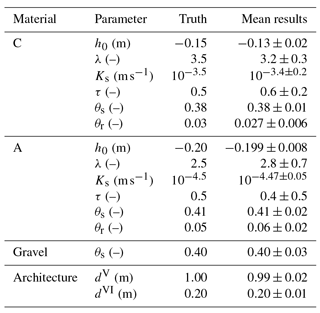
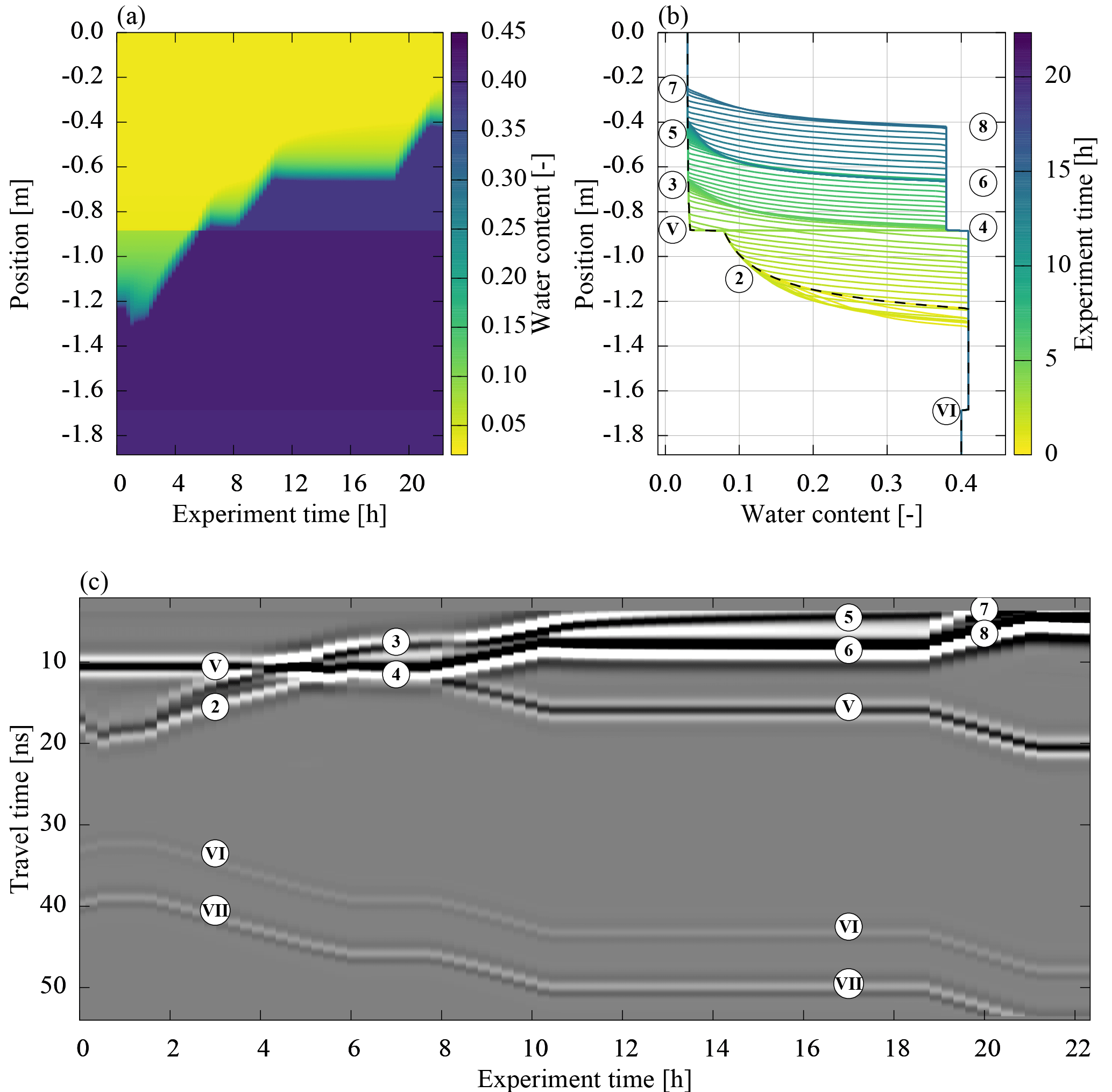
Figure 9The true synthetic data are simulated with hydraulic parameters that represent coarse-textured sandy soils (Table 2). (a) and (b) show different representations of the simulated water content. In (b) the initial water content distribution is marked with a black dashed line. (c) shows the simulation of the GPR signal. The imbibition leads to a characteristic transition zone reflection (marker (2)). The temporal evolution of this reflection is sensitive to the initial water content distribution, the soil water characteristic, and the hydraulic conductivity function. The data shown are processed according to Sect. 2.3 except for the normalization. In contrast to the data that are evaluated, the shown radargram is normalized to the maximum absolute amplitude of all traces, facilitating the visual comparison of the traces. The markers are defined in Fig. 14.
Initialized with static hydraulic equilibrium, the simulation starts with an initial drainage step where the groundwater table is lowered. Hence, the material at the upper end of the capillary fringe with high initial water content is desaturated. After the subsequent equilibration step, the groundwater table is raised during the subsequent imbibition step. The Brooks–Corey parameterization (Eq. 2) features a sharp kink where air enters the material at the upper end of the capillary fringe. Furthermore, the imbibition introduces an additional kink in the water content distribution (marker (2) in Fig. 9b), because the relaxation time from hydraulic non-equilibrium is much shorter for high water contents compared to the relaxation time for low water contents. This is due to the nonlinear dependency of the hydraulic conductivity (Eq. 3) on the water content leading to the differences in hydraulic conductivity of several orders of magnitude. Hence, the width of the transition zone is decreased during the imbibition phase.
During the equilibration step after the first imbibition, the additional kink smoothes. Thus, the water content increases in the material with low water content (3) and decreases in the material at the upper end of the capillary fringe (4). This smoothing depends on both the soil water characteristic and the hydraulic conductivity function. Sharpening and smoothing of the transition zone are repeated consistently for the other subsequent imbibition and equilibration phases (5–8).
According to the CRIM (Sect. 2.2.4), the relative permittivity distribution has the same shape as the water content distribution. Hence, kinks in the water content distribution directly induce partial reflections of the GPR signal (Fig. 9c). Shortly after starting the imbibition, the amplitude of the reflection at the additional kink (2) increases. After passing the material interface (V), the spatial distance of the kinks increases such that the two resulting reflection wavelets (3) and (4) are separable. Note that, since the water content changes continuously, the signal in-between these wavelets is a superposition of infinitesimal reflections which also contain information about the form of the transition zone. Additionally, the reflection (3) scans the initial water content distribution, which in steady state corresponds to the soil water characteristic. With progressing equilibration, the amplitude of reflection (3) decreases as the transition zone smoothes. The GPR signal of the subsequent imbibition and equilibration phases (5–8) show similar behavior and emphasize the relatively long timescale for hydraulic equilibration of sandy materials.
In summary, this numerical simulation confirms qualitatively (i) that the dynamics of the fluctuating groundwater table are sensitive to both the soil water characteristic and the hydraulic conductivity function and (ii) that the transition zone reflection leads to tractable reflections during the imbibition step.
3.2.2 Results and discussion
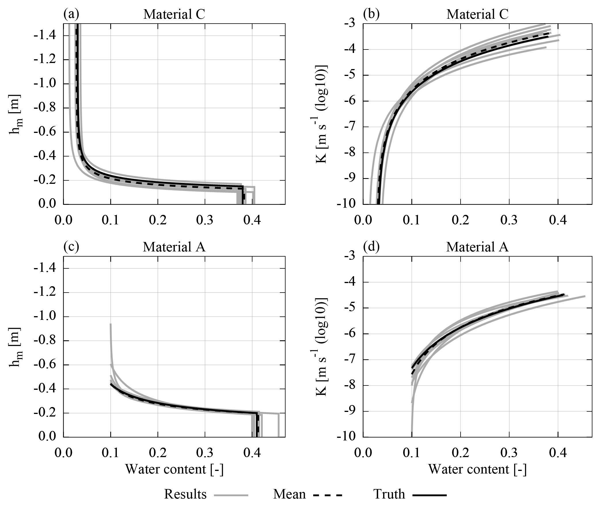
After the inversion of the synthetic data, we find that the resulting soil water characteristics for material A (Fig. 10a) exhibit a similar curvature but are shifted. Both the parameters h0 and λ influence the shape of the desaturated transition zone. Hence, merely evaluating the shape of the desaturated part of the transition zone is not necessarily sufficient to uniquely identify both parameters leading to large correlation coefficients. However, parameter h0 additionally determines the extent of the capillary fringe. If the evaluation is also sensitive to the extent of the capillary fringe, h0 can be uniquely identified, which significantly decreases the correlation between h0 and λ. Hence, we conclude that the strong correlation of the parameters and λC (−0.7, Fig. 11) indicates that the evaluation is more sensitive to the shape of the desaturated part of the transition zone than to the extent of the capillary fringe.
Since the architecture is a layered structure where material C is located above material A (Fig. 7), the water content in material C contributes to the travel time of the other reflections. This introduces correlations of with all the parameters associated with the soil water characteristic of material C. A high correlation of parameters indicates that the problem is not well-posed. This typically increases the number of local minima and thus the uncertainty of the parameters.

Figure 11The correlation coefficients for the mean parameter set show in particular that the porosity of the gravel layer () as well as the position of the material layers (dV and dVI) can be reliably estimated from single-offset GPR when evaluating both the signal travel time and amplitude.

Figure 12This figure shows (a) the water content distribution simulated with the resulting mean parameter set and (b) the difference to the true water content distribution (Fig. 9). The mean absolute deviation of the volumetric water content is 0.004. The overall balance of the volumetric water content can be characterized by calculating the mean of the summed difference per grid cell over all measurement times which yields −0.003. Hence, the mean parameter set generally underestimates the water content in the profile. The constant deviations above as well as below the groundwater table and in the gravel layer are due to small deviations in the estimated parameters , , , and . Still, the standard deviation of the estimated parameters contains the true parameter values (Table 2).
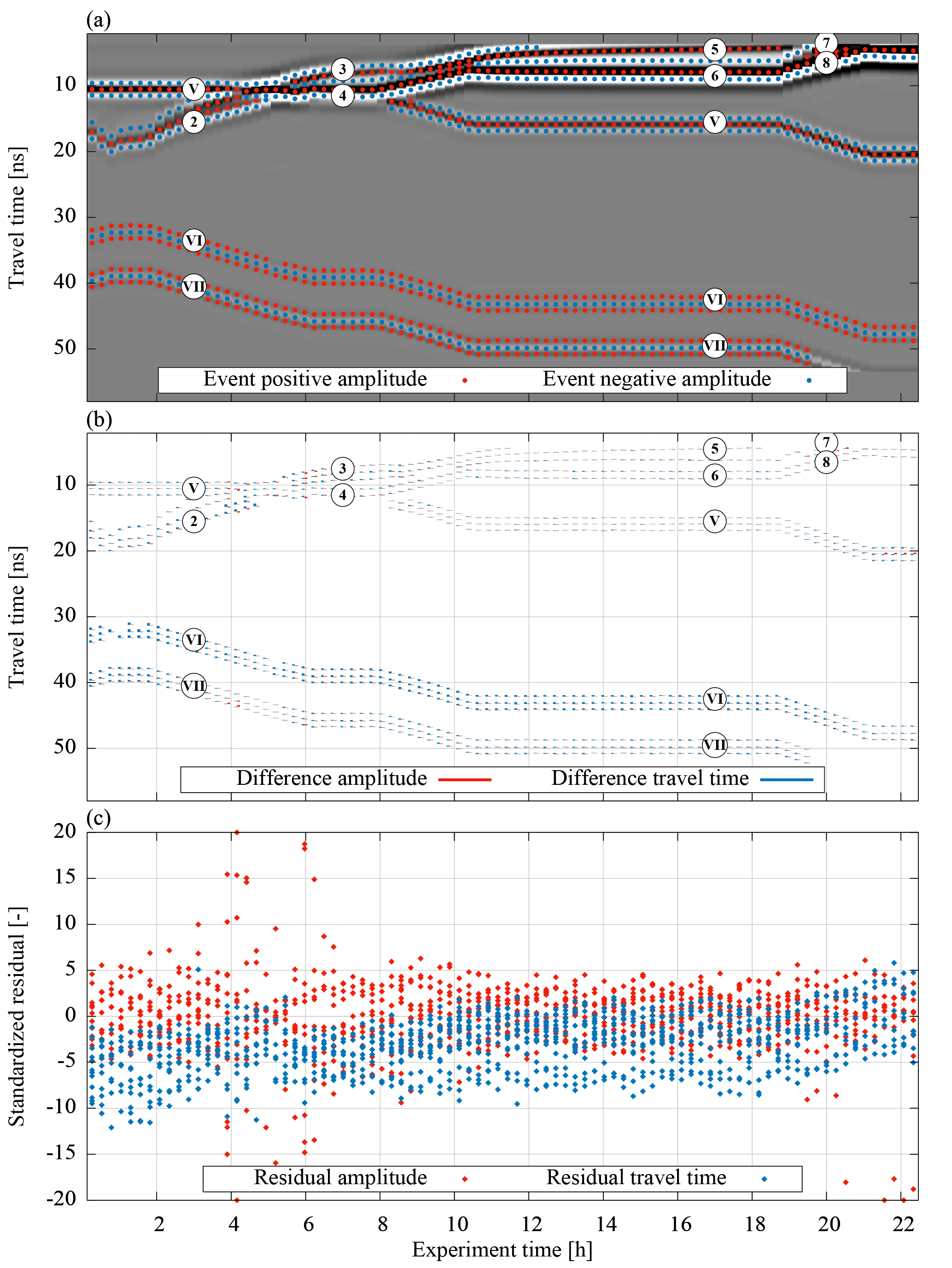
Figure 13The evaluation of the synthetic GPR data is separated into three parts (a) shows the selected events (Sect. 2.3.3) which are evaluated with the optimization. The data shown are processed according to Sect. 2.3 except for the normalization. In contrast to the data that are evaluated, the shown radargram is normalized to its maximum absolute amplitude, facilitating the visual comparison of the traces. (b) shows resulting differences in travel time and amplitude of the mean parameter set. The differences in amplitude are given in arbitrary units which are consistently used in this study. For the synthetic data, these differences are practically invisible. For the measured data, however, they are more clearly recognizable (Fig. 13). (c) shows standardized residuals (Eq. 8), essentially zooming into the small differences given in (b). Note that outliers are set onto the boundary. The markers are defined in Fig. 14.
The saturated hydraulic conductivity of material A (Fig. 10b) is approximately 1 order of magnitude smaller than the saturated hydraulic conductivity of material C (Table 2). Since the 1-D architecture is forced at the lower boundary, the hydraulic conductivity of material A limits the water flux into material C. Hence, the data are not sensitive to . Consequently, the uncertainty of the hydraulic conductivity in material C decreases for low water contents as the reflection at the additional kink (markers 3 and 5 in Fig. 9) is sensitive to the hydraulic conductivity. The hydraulic conductivity function (Eq. 3) is not unique if Ks is not fixed. This leads to a strong correlation of the parameters and τC (0.6, Fig. 11). Note that the uncertainty of the saturated hydraulic conductivity of material A also influences the uncertainty of the hydraulic conductivity of material C.
The uncertainty of the soil water characteristic of material A (Fig. 10c) is largest for low water contents, because there are only few data points available. In particular, this increases the uncertainty of λA (±0.7, Table 2). The material properties of the unsaturated material A are only monitored during the first ≈5 h of the experiment and are independent of the largest part of the other data. This regularizes the optimization leading to fewer local minima. Similar to material C, the parameters and λA are strongly correlated (−0.6). Yet, the uncertainty of is relatively small (±0.008, Table 2) mainly because it is essentially uncorrelated to other parameters. In contrast, the parameter is correlated to the parameters , λC, , and , because wrong parameters for material C introduce changes in the total water content which can be partially balanced out by adjusting .
The uncertainty of the saturated hydraulic conductivity of material A (Fig. 10d) is comparably small, because the largest fraction of the data are influenced by this parameter. Hence, the parameters τA and are only very weakly correlated.
The correlation coefficients (Fig. 11) also show that both the permittivity and the thickness of the gravel layer can be estimated reliably with the presented evaluation method using travel time and amplitude information of a single-offset time-lapse radargram. Evaluation methods that merely exploit the signal travel time (e.g., Gerhards et al., 2008) require a multichannel approach to achieve this goal.
In order to further investigate the quality of the mean parameter set, we simulated the resulting water content distribution (Fig. 12a) and subtracted the true water content distribution (Fig. 12b). Due to the narrow pore size distribution of the sandy material, small deviations in the parameters h0 and λ lead to large differences in the volumetric water content above the capillary fringe (). Combined with deviations in the position of the material interface, the largest differences in volumetric water content reach up to 0.17. Still, the mean absolute deviation of the volumetric water content is 0.004.
The remaining deviations in soil water content after the parameter estimation cause residuals in the GPR signal (Fig. 13). These residuals are most evident for the reflection at the gravel layer (VI). The bias of its travel time shows that the total water content above the gravel layer is underestimated with the mean parameter set. This bias is essentially balanced out with the properties of the gravel layer. However, the reflection originating from the basement of ASSESS (VII) reveals residuals that decrease as soon as the groundwater table is above the initial groundwater table. This indicates (i) deviations in the initial water content distribution and (ii) that the hydraulics during the initial drainage phase is not correctly represented.
Similar to the analysis of the deviation in water content (Fig. 12), the largest residuals in the unsaturated part of the domain are found where the groundwater table is crossing the interface of materials A and C. This indicates that the interference of those reflections still contains information which could not be exploited in the parameter estimation procedure.

Figure 14(a) A single-offset measurement of the hydraulic state of ASSESS (Fig. 1) at the beginning of the experiment is shown. For this measurement, the antenna was moved over the site at one point in time. The temporal evolution of the subsequent hydraulic dynamics was monitored with a stationary antenna at the position indicated with the vertical black line. The resulting time-lapse measurement data are shown in (b). Both radargrams are measured with internal channels with an antenna separation of 0.14 m. Except for the normalization, the data are processed according to Sect. 2.3. In contrast to the quantitative evaluation, the radargrams are normalized to their maximal absolute amplitude, facilitating the visual comparison of the traces. The markers – uppercase Roman numeral markers for material interfaces (I, II, III, IV, V, VI, and VII), lowercase Roman numeral markers for compaction interfaces (i, ii, iii, iv, and v), and markers with Arabic numerals for reflections originating from the water content distribution – are used consistently in this paper and are further explained in the text.
3.3 Measured data
In this section, the measured data (Sect. 2.2.4) are examined first qualitatively (Sect. 3.3.1). Afterwards, these data are used to estimate the subsurface architecture and the corresponding soil hydraulic material properties using the methods proposed in Sect. 2. The results of this inversion are discussed in Sect. 3.3.2.
3.3.1 Phenomenology
Before starting the experiment, a single-offset measurement was acquired to analyze the initial state of ASSESS revealing material interfaces as well as compaction interfaces (Fig. 14). Typically, it is difficult to associate the reflections based on an individual radargram. In particular, the reflection of the compaction interface (iv) close to the reflection of the initial position of the groundwater table (1) is difficult to distinguish from reflections originating from material interfaces.
ASSESS is confined by walls at all four sides. Reflections from confining walls are most visible around 1 m (W) but influence the signal for more than 2 m. The walls parallel to the measurement direction are approximately 4 m apart from each other. Thus, it is assumed that the measurement is also influenced by reflections originating from those walls. The reflection of the edge of the L-element (L) is particularly prominent.
As an aside, closer scrutiny of the radargrams reveals that the single-offset and the time-lapse data were measured with different but structurally identical antennas. Thus, in particular the measured GPR signals of the direct wave and the ground wave are slightly different.
The time-lapse GPR measurement was recorded at 17.05 m (Fig. 14b). As the groundwater table is raised, the reflection originating from the groundwater table (2) separates from the reflection of the compaction interface (iv). After passing the material interface, the reflection of the groundwater table (2) splits in two separate reflections, (3) and (4). This is due to the dependency of the hydraulic conductivity on the water content and was also identified for the synthetic data (Sect. 3.2.1). Since the transition zone is smoothing during the equilibration phase, the amplitude of reflection (3) decreases and the distance of the reflections (3) and (4) increases. During the subsequent imbibition step, the reflections are separated.
Corresponding to the analysis of the synthetic data (Sect. 3.2.1), the effects of the smoothing water content distribution are most clearly visible during the equilibration phase at the reflections (5) and (6). However, the associated measured signals interfere with the direct wave, the ground wave, and the reflection from the compaction interface (i) which makes the identification of these effects difficult. The reflections (7) and (8) measured during the final imbibition phase confirm the previous observations.
Together with the water content distribution, the time-lapse GPR data also contain information about the subsurface architecture. However, separating signal contribution from the subsurface architecture and the hydraulic dynamics is not always possible. Here, this is most prominent for the reflection of the material interface (V). Initially, the amplitude of this reflection is large, because the water content in material C is near the residual water content, whereas the water content in material A is significantly higher at the material interface. As soon as both materials are water saturated, the amplitude of the material interface reflection (V) is low since the effective porosities of the two materials are similar. Thus, the amplitude of the reflected signal originating from the material interfaces may change depending on the hydraulic state. Additional information about the subsurface architecture can be inferred from the reflection at the material interface between material A and the gravel layer (VI) and from the reflection at the material interface of the gravel layer and the concrete basement (VII). These reflections are in particular suitable to analyze the total change of water content over time.
In summary, we note that the characteristic properties of the transition zone reflection during the imbibition and equilibration steps that were identified in the simulation (Fig. 9) can also be identified in the measured data (Fig. 14).
3.3.2 Results and discussion
Since the GPR measurements cover only a small portion of the subsurface architecture of ASSESS, the hydraulic representation is restricted to 1-D (Sect. 3.1.1). Hence, 2-D effects such as lateral flow are neglected. This has to be considered during the event selection of measured data (Sect. 2.3.3). Therefore, the focus of this study is on evaluation of the imbibition phase of the experiment, because the effect of lateral flow in fluctuating groundwater table experiments is largest during drainage and close to the capillary fringe (Jaumann and Roth, 2017).
Investigating the resulting material properties of the inversion (Fig. 15), the main findings, which were discussed previously for the mean parameters for the synthetic data (Sect. 3.2.2), can also be identified for the measured data. These findings comprise (i) the shift in the soil water characteristic of material C, (ii) the large uncertainty of the saturated hydraulic conductivity of material C, (iii) the high uncertainty of the soil water characteristic of material A for low water contents, and (iv) the high sensitivity on .
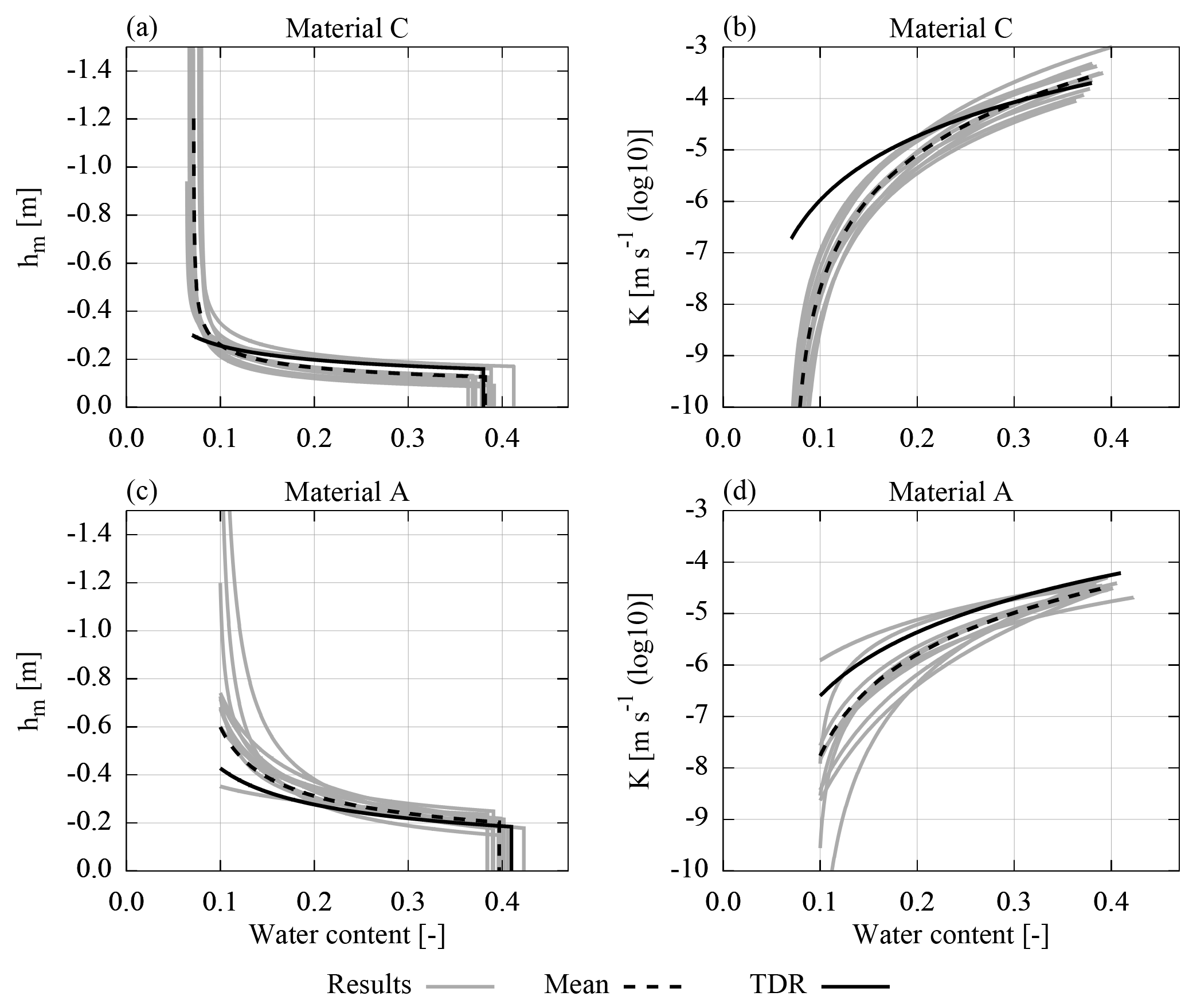
Figure 15The resulting material parameters estimated from measured data are shown for the 10 best ensemble members (Sect. 3.1.2) together with the mean of these parameter sets (Table 3) and a reference parameter set determined from TDR data acquired during the same experiment (Jaumann and Roth, 2017). The deviation from the reference parameters can be explained with representation errors in the GPR analysis (e.g., neglecting compaction interfaces) and missing data (e.g., for low water contents in material A). The plot range of the parameters is adjusted to the water content range of the corresponding data.
Table 3The mean and the standard deviation are calculated using the resulting parameters from the 10 best ensemble members (Sect. 3.1.2) estimated from measured data. The corresponding material functions are shown in Fig. 15. The reference parameters for the materials A and C are determined from TDR data acquired during the same experiment (Jaumann and Roth, 2017). Note that the standard deviations for these reference parameters are determined from a single Levenberg–Marquardt run and thus are only representative for one local minimum. Also, these standard deviations are given with the understanding that they are specific to the applied algorithm and will change for different algorithm parameters. Hence, these standard deviations are in particular not suitable to compare the precision of the TDR and GPR evaluation. For the TDR evaluation, the porosity of the materials is assumed to be known from core samples. The reference parameters for the subsurface architecture are calculated from ground truth measurements acquired during the construction of ASSESS. The corresponding standard deviations are given according to Buchner et al. (2012).
Compared to the uncertainties based on synthetic data (Table 2), the uncertainty of the resulting mean parameters (Table 3) mostly increased. Except for four parameters, the parameters estimated from TDR measurements (Jaumann and Roth, 2017) are within 1 standard deviation of the mean parameter set. The deviations of the other four parameters are clearly visible in Fig. 15 and will be analyzed in the following.
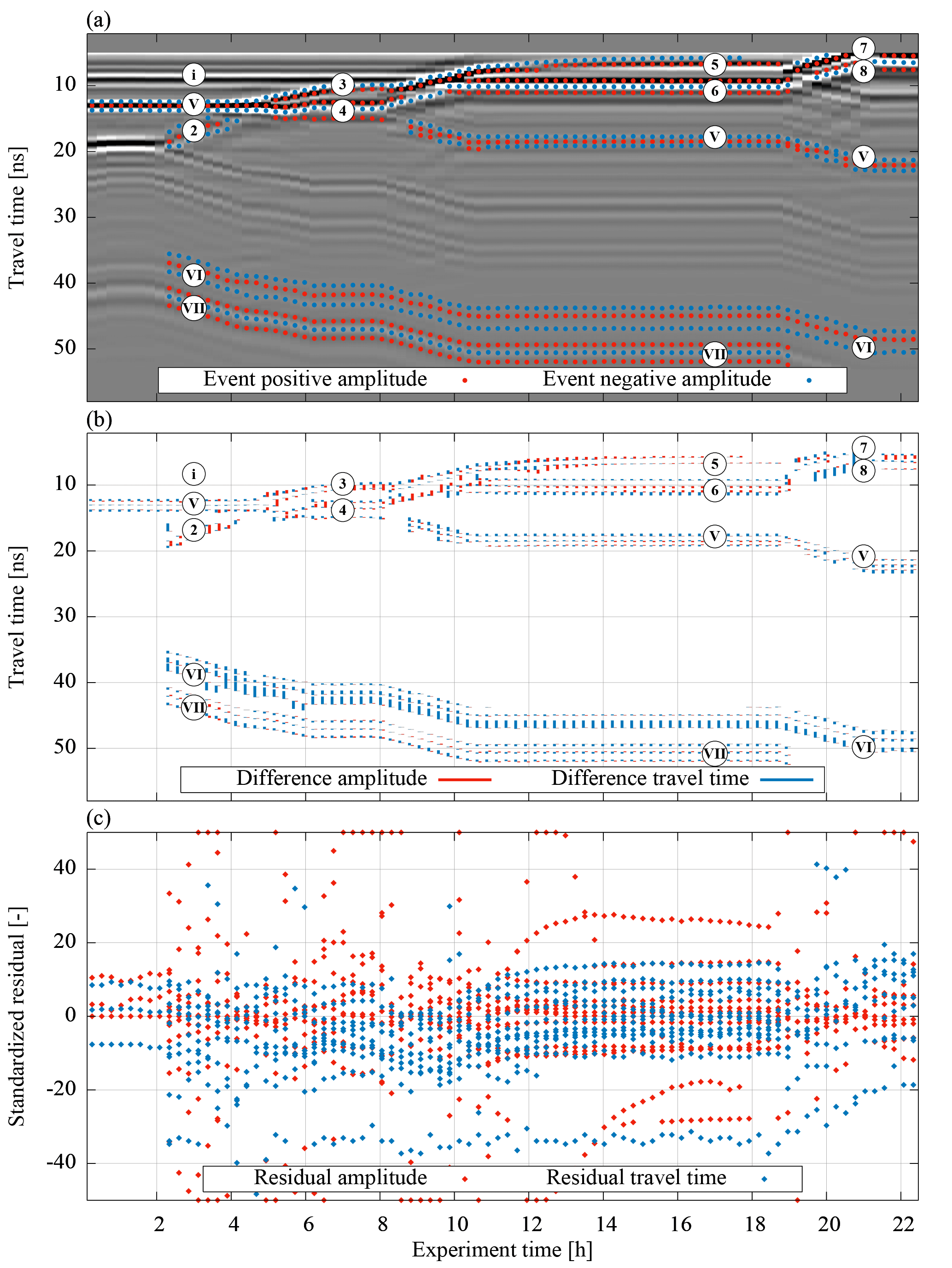
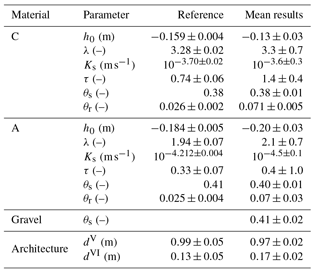
Figure 16Analogous to Fig. 13 but for measured data. Since the measurement data acquired with a stationary antenna cannot spatially resolve the lateral flow present in the initial drainage phase, the measured events of the hydraulic dynamics during the first 2 h are neglected.
The parameter estimated from the GPR data is approximately a factor of 3 larger than the estimated value based on the TDR data (Table 3). Essentially, there are three main reasons for this. First, by evaluating the travel time of reflection (V), integrated water content is included in the inversion. This also comprises the compaction interface (i) which is not represented in the model. At the beginning of the experiment, the amplitude of this reflection is comparable to the amplitude of the reflection originating from the interface of material A and C (V). Notice that the amplitude of the reflection (i) does not vanish, but merely decreases when the material is saturated at the end of the experiment (Fig. 14). This indicates that this reflection originates from changes in both the small-scale texture of the material and the stored water content at the beginning of the experiment. Hence, since this compaction interface is not represented in the model, the resulting is increased, coping for this representation error. Second, a deviation in the position of the groundwater table with reference to the antenna position at the surface can be partially adapted by changing . As the position of the surface is subject to change over the years, the measurements of the groundwater table are referenced to a fixed point at the end of the groundwater well, leaving the exact position of the surface relative to groundwater table uncertain. According to Buchner et al. (2012), the accuracy of the ASSESS architecture when compared to GPR measurements is ±0.05 m. The estimation of an offset to the Dirichlet boundary could mitigate this problem, but would in any case increase the number of local minima significantly making the optimization process less stable. Third, analyzing the TDR data, we find that an underestimation of is likely due to the lack of TDR measurements at low hydraulic potential. Hence, the sensitivity of the TDR data to is low.
The resulting value for parameter τC for the GPR evaluation is a factor of 2 larger compared to the evaluation of the TDR data. This parameter adjusts the hydraulic conductivity for the unsaturated material and is mainly determined with the reflections (3) and (5) originating from the additional kink during imbibition (Fig. 16). These reflections exhibit a small amplitude for low water contents. However, both reflections interfere with the rather prominent reflection originating from the compaction interface (i). Additionally, the reflection (5) also interferes with parts of the direct and the ground wave. Hence, the travel time of these reflections hardly changes, leading to an underestimation of the hydraulic conductivity for low water contents resulting in an overestimation of parameter τC.
Similar to parameter , the parameter estimated from the GPR data is approximately a factor of 3 smaller than the result from the TDR evaluation. However, this parameter can only be approximated evaluating the GPR data, because they lack events that are influenced by low water content.
The resulting value for parameter is smaller by a factor of 2 for the GPR evaluation than for the TDR evaluation. This parameter limits the flux through the lower boundary, because the domain is forced with a Dirichlet boundary condition. Hence, the parameter can be used to cope with errors in the boundary condition. Forcing ASSESS with a groundwater well instantiates a 3-D flux (Jaumann and Roth, 2017). Since this 3-D flux is not represented, the hydraulic potential at the bottom and thus also the water flux are too large. This is compensated by the parameter estimation with decreasing .
Concerning the position of the material interfaces, we find that the estimated interface position of material A and C (dV) corresponds well to the ground truth measurements acquired during the construction of the ASSESS site (Table 3). In contrast, the estimated position of the gravel layer (dVI) deviates from the ground truth measurements. However, the estimates are still within the uncertainty of the ground truth measurements when compared to GPR measurements.
An analysis of the remaining residuals in travel time after the optimization (Fig. 16b) shows that deviations in the width of the reflected wavelet contribute to the residuum significantly, in particular for reflections (V), (VI), and (VII). At the beginning of the experiment, the simulated wavelet is too broad for reflection (V), whereas it is too narrow for reflections (VI) and (VII). This is in particular noticeable for the residuals for reflection (VI) which are the major contribution to the cost function. Of all the events in this wavelet, the events with the longest travel time exhibit the largest residuals. The difference in the width of the reflected wavelet can be explained with the roughness of the material interfaces (Dagenbach et al., 2013). Due to the large grain size of the gravel, the real material interface is rougher than its representation. This also explains the partly non-symmetric broadening of the measured compared to the simulated wavelet of reflection (VI).
The measured reflection (6) interferes with the reflection of the compaction interface, (i) leading to a compressed reflected wavelet in the measurement. Similarly, reflections (3) and (5) also interfere with the compaction interface (i). Since interferences cannot be correctly evaluated if not all contributions are represented, this analysis shows that representing compaction interfaces is relevant in ASSESS.
As a side remark, note that the error originating from assuming a constant soil temperature for the calculation of the relative permittivity of water is relatively small regarding the total residuum. However, it is worth noting that the corresponding residuals easily exceed 1 standard deviation in signal travel time.
The distribution and the support of the measurement data (i) differs between the TDR sensors and GPR measurements (Fig. 1), (ii) relates directly to the applicability of the resulting parameters for the different evaluations, and (iii) influences the quantitative effect of different representation errors. In the reference analysis, the TDR sensors are distributed over a 2-D slice of ASSESS measuring in all available materials (Fig. 1). Yet, their measurement volume is limited to the position of the sensors yielding the average permittivity along the central TDR rod of each sensor. Hence, these measurements are subject to representation errors such as small-scale heterogeneity or uncertainty of the sensor position (Jaumann and Roth, 2017). In contrast, the GPR measurements do not cover the whole ASSESS test site and their support is dependent on the evaluated events of the wavelet. This includes the whole depth average (travel time) and the contrast (amplitude) of both the permittivity and electrical conductivity. Hence, these measurement data are subject to representation errors such as neglected compaction interfaces and the roughness of the material interfaces. Hence, the previous analysis illustrates how GPR-determined parameters can differ from TDR-determined ones, making joint evaluation procedures both challenging and promising since they open a window to the soils' multi-scale nature.
TDR measurements are a standard method that provides measurement data for the estimation of soil hydraulic material properties. However, this invasive measurement method yields point-scale measurements and typically requires a local measurement station. Hence, it is difficult to apply at larger scales or to transfer the sensors to another field site. In contrast, GPR is a noninvasive measurement method that is traditionally used for subsurface characterization including subsurface architecture and effective water content. The analysis of GPR measurements is much more challenging than that of TDR and there is still a need for efficient quantitative evaluation methods.
In this study, we propose a new heuristic semiautomatic evaluation approach to identify, extract, and associate relevant information from GPR data. Focussing the optimization on this relevant information regularizes the parameter estimation. The suitability of the proposed methods to accurately identify the subsurface architecture and the soil hydraulic material properties was analyzed for synthetic and measured time-lapse GPR data.
The developed GPR data evaluation method first detects the most important extrema of the signal (events) in the measurement and in the simulation. Subsequently, the detected measured events are associated with the detected simulated events. All plausible combinations of simulated and measured events are analyzed to identify the optimal pair association of these events. To decrease the computational effort, the detected events are grouped in clusters. First, the clusters are associated. Then follows the association of the events contained in these clusters. In order to estimate the subsurface architecture and the corresponding soil hydraulic material properties, the difference in the signal travel time and amplitude of the associated events is minimized with inversion methods. Using events instead of the full GPR signal regularizes the optimization.
Synthetic and measured single-offset time-lapse GPR data are first analyzed qualitatively. It was confirmed that a fluctuating groundwater table experiment introduces characteristic transition zone reflections that are likely to provide valuable information for the parameter estimation. Subsequently, the subsurface architecture and soil hydraulic material properties are estimated based on the GPR data using a global–local parameter estimation approach with preconditioning. The preconditioning step starts from an ensemble of 60 Latin-hypercube-sampled initial parameters sets. They are used to initialize a preconditioning step in which a simulated annealing algorithm and a Levenberg–Marquardt algorithm are sequentially coupled. In this step, these algorithms optimize parameters based on a subsampled data set with a limited number of iterations. The resulting parameter sets are then used to initialize the Levenberg–Marquardt algorithm that operates on the full data set.
Employing the presented approaches on synthetic data shows that the true parameters are within 1 standard deviation of the resulting mean parameter set based on the 10 best ensemble members. This mean parameter set describes the hydraulic dynamics with a mean absolute error in volumetric water content of 0.004. Additionally, we found that the parameter correlations are mostly specific to the experiment type and the subsurface architecture. Using travel time and amplitude information in the evaluation allowed to estimate the effective permittivity and layer depth simultaneously with a single GPR channel.
The resulting parameters for the measured data are mostly consistent with results from reference TDR measurement data. We discussed the deviations of the parameters and basically associated them with representation errors and the lack of available measurement data. Relevant representation errors in the GPR data analysis comprise in particular the neglected (i) compaction interfaces and (ii) roughness of the material interfaces.
The three major drawbacks of the presented approach comprise (i) the computational effort which is required to solve Richards' and Maxwell's equations, (ii) the limited number of events that can be analyzed due to the pairwise event association which investigates all plausible combinations of simulated and measured events, and (iii) the fact that the hyperparameters for the GPR evaluation algorithm have to be determined a priori. The latter is difficult and requires expert knowledge, especially as the shape of the radargram is likely to change considerably during the optimization procedure.
Although, the proposed methods have been shown in 1-D, going to 2-D and even to 3-D is first and foremost a matter of computational effort with 2-D already demanding significant time on a large compute cluster. No concepts or methods beyond what we demonstrated in this paper are required, however.
Previous work showed that the location of moderately complicated layer interfaces and of the mean water content between them can be obtained from multi-offset measurements (Buchner et al., 2012). Together with the demonstration in this paper that the effective hydraulic material properties of layers can be estimated from single-offset time-lapse measurements, we now have the methods to determine the subsurface architecture and its hydraulic properties for moderately complicated situations. This obviously demands quite a significant experimental effort together with subsequent massive computations, as spatially resolved time-lapse measurements of the region of interest are required which then have to be inverted.
SJ designed and conducted the experiment, developed the main ideas, implemented the algorithms, and analyzed the measurement data. KR contributed with guiding discussions. SJ prepared the manuscript with contributions of both authors.
We thank Jens S. Buchner for software to process (i) the raw data of the
ASSESS architecture and (ii) GPR data according to the constructive
inversion approach. We are grateful to Angelika Gassama for technical
assistance with respect to ASSESS. We especially thank Patrick Klenk and
Elwira Zur for assistance during the experiment. The authors acknowledge
support by the state of Baden-Württemberg through bwHPC and the German
Research Foundation (DFG) through grants INST 35/1134-1 FUGG and
RO 1080/12-1. We are also grateful to the editor Insa Neuweiler and to two
anonymous referees, who helped to improve the manuscript significantly.
Edited by: Insa Neuweiler
Reviewed by: two anonymous referees
Bauser, H. H., Jaumann, S., Berg, D., and Roth, K.: EnKF with closed-eye period – towards a consistent aggregation of information in soil hydrology, Hydrol. Earth Syst. Sci., 20, 4999–5014, https://doi.org/10.5194/hess-20-4999-2016, 2016. a
Birchak, J. R., Gardner, C. G., Hipp, J. E., and Victor, J. M.: High dielectric constant microwave probes for sensing soil moisture, Proc. IEEE, 62, 93–98, https://doi.org/10.1109/PROC.1974.9388, 1974. a
Bleistein, N.: Two-and-one-half dimensional in-plane wave propagation, Geophys. Prospect., 34, 686–703, https://doi.org/10.1111/j.1365-2478.1986.tb00488.x, 1986. a
Bradford, J., Thoma, M., and Barrash, W.: Estimating hydrologic parameters from water table dynamics using coupled hydrologic and ground-penetrating radar inversion, in: Proceedings of the 15th International Conference on Ground Penetrating Radar, 30 June–4 July 2014, Brussels, Belgium, 232–237, https://doi.org/10.1109/ICGPR.2014.6970420, 2014. a, b, c
Brooks, R. H. and Corey, A. T.: Properties of porous media affecting fluid flow, J. Irrig. Drain. Div.-ASCE, 92, 61–90, 1966. a
Buchner, J. S., Wollschläger, U., and Roth, K.: Inverting Surface GPR Data using FDTD Simulation and Automatic Detection of Reflections to Estimate Subsurface Water Content and Geometry, Geophysics, 77, H45–H55, https://doi.org/10.1190/geo2011-0467.1, 2012. a, b, c, d, e, f, g, h, i, j, k
Busch, S., van der Kruk, J., Bikowski, J., and Vereecken, H.: Quantitative conductivity and permittivity estimation using full-waveform inversion of on-ground GPR data, Geophysics, 77, H79–H91, https://doi.org/10.1190/geo2012-0045.1, 2012. a, b, c, d
Carmichael, R. S.: Physical properties of rocks and minerals, CRC Press, Boca Raton, 1989. a
Dagenbach, A., Buchner, J. S., Klenk, P., and Roth, K.: Identifying a parameterisation of the soil water retention curve from on-ground GPR measurements, Hydrol. Earth Syst. Sci., 17, 611–618, https://doi.org/10.5194/hess-17-611-2013, 2013. a, b, c
Daniels, D.: Ground Penetrating Radar, 2ne Edn., The Institution of Engineering and Technology, London, UK, https://doi.org/10.1049/PBRA015E, 2004. a
Duan, Q., Sorooshian, S., and Gupta, V.: Effective and efficient global optimization for conceptual rainfall-runoff models, Water Resour. Res., 28, 1015–1031, https://doi.org/10.1029/91WR02985, 1992. a
Ernst, J. R., Green, A. G., Maurer, H., and Holliger, K.: Application of a new 2D time-domain full-waveform inversion scheme to crosshole radar data, Geophysics, 72, J53–J64, https://doi.org/10.1190/1.2761848, 2007. a
Farjadpour, A., Roundy, D., Rodriguez, A., Ibanescu, M., Bermel, P., Joannopoulos, J. D., Johnson, S. G., and Burr, G. W.: Improving accuracy by subpixel smoothing in the finite-difference time domain, Opt. Lett., 31, 2972–2974, https://doi.org/10.1364/OL.31.002972, 2006. a
Gerhards, H., Wollschläger, U., Yu, Q., Schiwek, P., Pan, X., and Roth, K.: Continuous and simultaneous measurement of reflector depth and average soil-water content with multichannel ground-penetrating radar, Geophysics, 73, J15–J23, https://doi.org/10.1190/1.2943669, 2008. a, b
Giannopoulos, A.: Modelling ground penetrating radar by GprMax, Constr. Build. Mater., 19, 755–762, https://doi.org/10.1016/j.conbuildmat.2005.06.007, 2005. a
Heimovaara, T. J., Focke, A. G., Bouten, W., and Verstraten, J. M.: Assessing Temporal Variations in Soil Water Composition with Time Domain Reflectometry, Soil Sci. Soc. Am. J., 59, 689–698, https://doi.org/10.2136/sssaj1995.03615995005900030009x, 1995. a
Hopmans, J. W., Šimůnek, J., Nunzio, R., and Wolfgang, D.: Simultaneous determination of water transmission and retention properties. Inverse Methods, in: Methods of Soil Analysis, Part 4. Physical Methods, edited by: Dane, J. and Topp, G. C., Soil Science Society of America Book Series, Madison, Wisconsin, USA, 963–1008, 2002. a
Huyer, W. and Neumaier, A.: Global Optimization by Multilevel Coordinate Search, J. Global Optim., 14, 331–355, https://doi.org/10.1023/A:1008382309369, 1999. a
Ippisch, O., Vogel, H.-J., and Bastian, P.: Validity Limits for the van Genuchten-Mualem Model and Implications for Parameter Estimation and Numerical Simulation, Adv. Water Resour., 29, 1780–1789, https://doi.org/10.1016/j.advwatres.2005.12.011, 2006. a
Jackson, J. D.: Classical Electrodynamics, 3rd Edn., John Wiley and Sons Inc., New Jersey, USA, 1999. a
Jadoon, K. Z., Weihermüller, L., Scharnagl, B., Kowalsky, M. B., Bechtold, M., Hubbard, S. S., Vereecken, H., and Lambot, S.: Estimation of soil hydraulic parameters in the field by integrated hydrogeophysical inversion of time-lapse ground-penetrating radar data, Vadose Zone J., 11, 1375–1379, https://doi.org/10.1190/1.3255105, 2012. a, b, c
Jaumann, S.: http://ts.iup.uni-heidelberg.de/data/jaumann-roth-2017-gpr-hess.zip (last access: 23 April 2018), 2017. a
Jaumann, S. and Roth, K.: Effect of unrepresented model errors on estimated soil hydraulic material properties, Hydrol. Earth Syst. Sci., 21, 4301–4322, https://doi.org/10.5194/hess-21-4301-2017, 2017. a, b, c, d, e, f, g, h
Jonard, F., Weihermüller, L., Schwank, M., Jadoon, K. Z., Vereecken, H., and Lambot, S.: Estimation of Hydraulic Properties of a Sandy Soil Using Ground-Based Active and Passive Microwave Remote Sensing, IEEE T. Geosci. Remote, 53, 3095–3109, https://doi.org/10.1109/TGRS.2014.2368831, 2015. a, b, c
Kaatze, U.: Complex permittivity of water as a function of frequency and temperature, J. Chem. Eng. Data, 34, 371–374, https://doi.org/10.1021/je00058a001, 1989. a
Klenk, P., Jaumann, S., and Roth, K.: Quantitative high-resolution observations of soil water dynamics in a complicated architecture using time-lapse ground-penetrating radar, Hydrol. Earth Syst. Sci., 19, 1125–1139, https://doi.org/10.5194/hess-19-1125-2015, 2015. a, b
Lambot, S., Antoine, M., Van den Bosch, I., Slob, E., and Vanclooster, M.: Electromagnetic inversion of GPR signals and subsequent hydrodynamic inversion to estimate effective vadose zone hydraulic properties, Vadose Zone J., 3, 1072–1081, https://doi.org/10.2113/3.4.1072, 2004. a
Lambot, S., Slob, E., Rhebergen, J., Lopera, O., Jadoon, K. Z., and Vereecken, H.: Remote estimation of the hydraulic properties of a sand using full-waveform integrated hydrogeophysical inversion of time-lapse, off-ground GPR data, Vadose Zone J., 8, 743–754, https://doi.org/10.2136/vzj2008.0058, 2009. a, b, c
Lampe, B., Holliger, K., and Green, A. G.: A finite-difference time-domain simulation tool for ground-penetrating radar antennas, Geophysics, 68, 971–987, https://doi.org/10.1190/1.1581069, 2003. a
Léger, E., Saintenoy, A., and Coquet, Y.: Estimating saturated hydraulic conductivity from ground-based GPR monitoring Porchet infiltration in sandy soil, in: Proceedings of the 15th International Conference on Ground Penetrating Radar, 30 June–4 July 2014, Brussels, Belgium, 124–130, https://doi.org/10.1109/ICGPR.2014.6970399, 2014. a, b, c
Léger, E., Saintenoy, A., Tucholka, P., and Coquet, Y.: Inverting surface GPR data to estimate wetting and drainage water retention curves in laboratory, in: Advanced Ground Penetrating Radar (IWAGPR), 2015 8th International Workshop on IEEE, 7–10 July 2015, Florence, Italy, 1–5, https://doi.org/10.1109/IWAGPR.2015.7292672, 2015. a, b, c, d
Looms, M. C., Binley, A., Jensen, K. H., Nielsen, L., and Hansen, T. M.: Identifying Unsaturated Hydraulic Parameters Using an Integrated Data Fusion Approach on Cross-Borehole Geophysical Data, Vadose Zone J., 7, 238–248, https://doi.org/10.2136/vzj2007.0087, 2008. a
Manoli, G., Rossi, M., Pasetto, D., Deiana, R., Ferraris, S., Cassiani, G., and Putti, M.: An iterative particle filter approach for coupled hydro-geophysical inversion of a controlled infiltration experiment, J. Comput. Phys., 283, 37–51, https://doi.org/10.1016/j.jcp.2014.11.035, 2015. a
Metropolis, N., Rosenbluth, A. W., Rosenbluth, M. N., Teller, A. H., and Teller, E.: Equation of state calculations by fast computing machines, J. Chem. Phys., 21, 1087–1092, 1953. a
Moghadas, D., Jadoon, K. Z., Vanderborght, J., Lambot, S., and Vereecken, H.: Estimation of the near surface soil water content during evaporation using air-launched ground-penetrating radar, Near Surf. Geophys., 12, 623–633, https://doi.org/10.3997/1873-0604.2014017, 2014. a, b
Mualem, Y.: A new Model for Predicting the Hydraulic Conductivity of Unsaturated Porous Media, Water Resour. Res., 12, 513–522, https://doi.org/10.1029/WR012i003p00513, 1976. a
Neal, A.: Ground-penetrating radar and its use in sedimentology: principles, problems and progress, Earth-Sci. Rev., 66, 261–330, https://doi.org/10.1016/j.earscirev.2004.01.004, 2004. a
Nelder, J. A. and Mead, R.: A Simplex Method for Function Minimization, Comput. J., 7, 308–313, https://doi.org/10.1093/comjnl/7.4.308, 1965. a
Oskooi, A. F., Roundy, D., Ibanescu, M., Bermel, P., Joannopoulos, J. D., and Johnson, S. G.: MEEP: A flexible free-software package for electromagnetic simulations by the FDTD method, Comput. Phys. Commun., 181, 687–702, https://doi.org/10.1016/j.cpc.2009.11.008, 2010. a
Press, W. H.: Numerical recipes 3rd edition: The art of scientific computing, Cambridge University Press, Cambridge, 2007. a, b
Richards, L. A.: Capillary Conduction of Liquids through Porous Mediums, Physics, 1, 318–333, https://doi.org/10.1063/1.1745010, 1931. a
Robinson, D., Jones, S. B., Wraith, J., Or, D., and Friedman, S.: A review of advances in dielectric and electrical conductivity measurement in soils using time domain reflectometry, Vadose Zone J., 2, 444–475, https://doi.org/10.2136/vzj2003.4440, 2003. a
Rossi, M., Manoli, G., Pasetto, D., Deiana, R., Ferraris, S., Strobbia, C., Putti, M., and Cassiani, G.: Coupled inverse modeling of a controlled irrigation experiment using multiple hydro-geophysical data, Adv. Water Resour., 82, 150–165, https://doi.org/10.1016/j.advwatres.2015.03.008, 2015. a, b
Scholer, M., Irving, J., Binley, A., and Holliger, K.: Estimating vadose zone hydraulic properties using ground penetrating radar: The impact of prior information, Water Resour. Res., 47, w10512, https://doi.org/10.1029/2011WR010409, 2011. a, b
Taflove, A. and Hagness, S.: Computational Electrodynamics: The Finite-Difference Time-Domain Method, 2nd Edn., Artech House, Norwood, MA, USA, 2000. a
Thoma, M. J., Barrash, W., Cardiff, M., Bradford, J., and Mead, J.: Estimating Unsaturated Hydraulic Functions for Coarse Sediment from a Field-Scale Infiltration Experiment, Vadose Zone J., 13, https://doi.org/10.2136/vzj2013.05.0096, 2014. a, b
Tran, A. P., Vanclooster, M., Zupanski, M., and Lambot, S.: Joint estimation of soil moisture profile and hydraulic parameters by ground-penetrating radar data assimilation with maximum likelihood ensemble filter, Water Resour. Res., 50, 3131–3146, https://doi.org/10.1002/2013WR014583, 2014. a
Vrugt, J. A., Stauffer, P. H., Wöhling, T., Robinson, B. A., and Vesselinov, V. V.: Inverse modeling of subsurface flow and transport properties: A review with new developments, Vadose Zone J., 7, 843–864, https://doi.org/10.2136/vzj2007.0078, 2008. a