Assessment of uncertainties in soil erosion and sediment yield estimates at ungauged basins: an application to the Garra River basin, India

High soil erosion and excessive sediment load are serious problems in several Himalayan river basins. To apply mitigation procedures, precise estimation of soil erosion and sediment yield with associated uncertainties are needed. Here, the revised universal soil loss equation (RUSLE) and the sediment delivery ratio (SDR) equations are used to estimate the spatial pattern of soil erosion (SE) and sediment yield (SY) in the Garra River basin, a small Himalayan tributary of the River Ganga. A methodology is proposed for quantifying and propagating uncertainties in SE, SDR and SY estimates. Expressions for uncertainty propagation are derived by first-order uncertainty analysis, making the method viable even for large river basins. The methodology is applied to investigate the relative importance of different RUSLE factors in estimating the magnitude and uncertainties in SE over two distinct morphoclimatic regimes of the Garra River basin, namely the upper mountainous region and the lower alluvial plains. Our results suggest that average SE in the basin is very high (23 ± 4.7 t ha⁻¹ yr⁻¹) with higher values in the upper mountainous region (92 ± 15.2 t ha⁻¹ yr⁻¹) compared to the lower alluvial plains (19.3 ± 4 t ha⁻¹ yr⁻¹). Furthermore, the topographic steepness (LS) and crop practice (CP) factors exhibit higher uncertainties than other RUSLE factors. The annual average SY is estimated at two locations in the basin – Nanak Sagar Dam (NSD) for the period 1962–2008 and Husepur gauging station (HGS) for 1987–2002. The SY at NSD and HGS are estimated to be 6.9 ± 1.2 × 10⁵ t yr⁻¹ and 6.7 ± 1.4 × 10⁶ t yr⁻¹, respectively, and the estimated 90 % interval contains the observed values of 6.4 × 10⁵ t yr⁻¹ and 7.2 × 10⁶ t yr⁻¹, respectively. The study demonstrated the usefulness of the proposed methodology for quantifying uncertainty in SE and SY estimates at ungauged basins.

1 Introduction

Soil erosion is a serious problem, which not only causes land degradation and loss of agricultural productivity but also alters geomorphic processes and sediment fluxes in a river basin. Estimation of soil erosion (SE) and sediment yield (SY) of a river basin are therefore essential for agricultural planning and river management. SE and SY can be estimated by either empirical models that are developed solely based on experimental studies (variants of universal soil loss equations e.g., USLE, RUSLE and MUSLE universal soil loss equations) or process-based models that are based on parameterization of physical processes, e.g., the Water Erosion Prediction Project (WEPP); Chemicals, Runoff, and Erosion from Agricultural Management Systems (CREAMS) and Agricultural Nonpoint Source (AGNPS). While the process-based models may be more reliable and appealing, the empirical models are popular because they can be applied on basins with no or limited data (Merritt et al., 2003).

The estimates of SE and SY alone are not sufficient for effectively addressing the soil erosion problem in a river basin. One needs to quantify uncertainties in those estimates as well. These uncertainties can stem from input data (measurement errors, coarse spatial and temporal resolution, missing values), model (parameter, structural, and algorithmic or numerical uncertainty), and stochastic nature of the soil erosion process (Beven and Brazier, 2011; JCGM, 2008). Since quantification of all the sources of uncertainties is difficult, studies make assumptions about their relative importance and mutual independence. Nevertheless, to the best of the authors' knowledge, no unified approach is available to quantify uncertainty in SE and SY estimates for ungauged basins. The following paragraphs briefly review the literature on the uncertainty estimates of SE and SY and highlight the existing gaps.

Arguably, the most popular empirical model for estimating SE is USLE (universal soil loss equation) and its variants such as RUSLE (revised) and MUSLE (modified). Variations in USLE are also used in distributed hydrological models like the Evaluation of the Water Quality Model (EUTROMOD), the Soil and Water Assessment Tool (SWAT) and the Simulator for Water Resources in Rural Basins (SWRRB). The USLE estimates sheet and rill erosion but does not account for gully or channel erosion in a basin. Developed in the 1960s with more than 10 000 plots per year data from the USA, the method was designed for estimating long-term SE at a plot-scale, but it is now frequently used for estimating erosion at a basin-scale, albeit with some modifications. This study uses the RUSLE model that estimates SE by considering five factors, namely rainfall and runoff erosivity (R factor), soil erodibility (K factor), topography (LS factor), cover and management (C factor), and support practice (P factor).

The studies on uncertainty analysis of the RUSLE can be divided into three groups:

• Studies that have quantified uncertainties in individual factors of the RUSLE. For example, Wang et al. (2002b) quantified spatial uncertainty in the R factor by using geostatistics. Catari et al. (2011) assessed uncertainty in the R factor by comparing traditional methods with at-site measurements. Torri et al. (1997), Wang et al. (2001) and Parysow et al. (2003) investigated uncertainty in the K factor by using geostatistical methods. Gertner et al. (2002), Wang et al. (2002a), Wu et al. (2005) and Mondal et al. (2016) estimated uncertainty in the LS factor based on at-site measurements and cell variation in the digital elevation model (DEM).

• Studies that have used backward or inverse uncertainty propagation in which modeled and observed values of SE are compared to evaluate model biases, check a model's suitability for a basin, and estimate model parameters (Risse et al., 1993; Falk et al., 2010 and Carmona et al., 2017). The backward uncertainty analysis requires observed values of SE, and hence not applicable for ungauged basins.

• Studies that have used forward uncertainty propagation in which uncertainties present in input data and/or the model are propagated to quantify uncertainties in the SE estimates. A few studies (Hession et al., 1996; Biesemans et al., 2000; Tetzlaff and Wendland, 2012; Tetzalf et al., 2013) that are relevant for this work are summarized below.

Hession et al. (1996) presented a two-phase Monte Carlo methodology for forward propagation of uncertainty and demonstrated its application at an experiential plot in Oklahoma, USA. They divided uncertainty in USLE factors into knowledge uncertainty and natural stochastic variability and argued that the two types of uncertainties should be analyzed separately to draw useful conclusions. They considered knowledge uncertainty for the R factor, stochastic variability for the K and C factors, and treated LS and P factors as constants. They also studied the effect of spatial discretization in models and the assumption of independence of parameters on uncertainty quantification. However, since information on dependence of USLE factors was not available, they assumed different levels of correlation among them.

Biesemans et al. (2000) applied a Monte Carlo error propagation technique for estimating uncertainty in SE and SY (referred to as off-site sediment accumulation) at a watershed in Belgium. Elevation data were assumed to have auto-correlated errors, which were modeled using fractional Gaussian noise to estimate uncertainty in the LS factor. Soil texture and its organic content were measured at 153 locations in the watershed to estimate the K factor. The K factors so obtained were interpolated using Kriging. The variance of the Kriging surface was taken as a measure of K-factor uncertainty. The C factor was assumed to have a uniform distribution with minimum and maximum values estimated based on a USLE table and by appropriately weighing the C factor for each crop by the erosivity value in its growing season. R and P factors were assumed constant. The result showed that the observed value of SE lies within one standard error of the estimated mean value, prompting authors to conclude that RUSLE is a suitable model for their study watershed and that the RUSLE model should use probability distribution of input factors rather than their fixed values.

Tetzlaff and Wendland (2012) and Tetzalf et al. (2013) performed forward uncertainty analysis on the ABAG model (an adaptation of USLE to German conditions) by using Gaussian error propagation and Monte Carlo simulations. ABAG was a part of the MEPhos model that was applied to determine SY for the state of Hesse in Germany (21 115 km²). However, because of high computational cost, the uncertainty analysis for SE using ABAG was performed for a relatively small catchment of the river Gersprenz (485 km²). The uncertainty in the LS factor was estimated as standard deviation of 1000 LS factors derived from 1000 simulated DEM surfaces obtained by adding random Gaussian error to the original DEM. Uncertainties for the other USLE factors were assumed (R uncertainty of 10 %, C of 23 % and K of 10 %) based on auxiliary information, and the P factor was treated as constant. The authors calculated that the uncertainty in USLE factors resulted in 34 % uncertainty in the mean annual soil loss estimates.

Not all of the sediment eroded in a basin is delivered out of it; a significant portion of the eroded material gets deposited at intermediate locations. Sediment yield (SY) denotes the total sediment outflow from a basin over a specified duration. It is usually measured by either stream flow sediment sampling or a reservoir sedimentation survey. By definition, SY includes both bed load and suspended load. However, since streamflow sediment sampling is often restricted to suspended load, the SY estimates from streamflow sampling are usually adjusted upward by some empirical procedure (e.g., Table 3.2 of Vanoni, 1975).

Reviews on SY modeling suggest that unlike SE modeling, no universal relationships are available that can be applied to every situation, rather a region-specific relationship is considered to be the best method for predicting SY (Ludwig and Probst, 1998; De Vente et al., 2011). The most common approach to predict SY is to estimate it as a product of gross SE and sediment delivery ratio (SDR; Walling, 1983; Richards, 1993), where SDR is defined as the ratio of SY at a prediction location to the gross or total SE of a basin whose outlet is the prediction location. Precise estimate of SDR is not available, but it is primarily related to the drainage basin area (USDA, 1972; De Vente et al., 2007). According to Boyce (1975), SDR generally decreases with increasing basin area because with an increase in basin size mean slope decreases and sediment storage locations between source areas and the basin outlet increases. The most favored method for long-term SY estimation is the USLE-SDR method where gross SE is estimated by the USLE model (e.g., Ebisemiju, 1990; Walling, 1993; Van et al., 2001; Amore et al., 2004; Bhattarai and Dutta, 2007; Boomer et al., 2008). This study uses the RUSLE-SDR model for predicting SY, in which SDR is obtained as a function of basin area based on the equation developed for north Indian river basins by Sharda and Ojasvi (2016).

Only a few studies have reported uncertainty in SY estimates by using the USLE-SDR approach. Ferro and Porto (2000) and Stefano and Ferro (2007) quantified uncertainty in the estimates of SY for river basins in Italy using a USLE-SDR-based model termed the sediment delivery distributed (SEDD) model. The model could predict SY at event and annual scales, but requires observed data for its calibration and hence not suitable for ungauged basins. Catari (2010) used the RUSLE-SDR model to investigate uncertainty in the estimates of SY for the upper Llobregat River basin in Spain. The uncertainties in individual RUSLE factors and SDR are first quantified and then added in quadrature to estimate uncertainty in SY. The LS and C factors were found to have the major influence on SY uncertainty.

The literature review on SE and SY estimation described in the foregoing paragraphs suggest that (i) very few studies have computed uncertainties in SE and SY for ungauged basins. Most of the existing studies are either restricted to the plot-scale or are carried out for basins with measured data; (ii) while the importance of sediment erosion in Himalayan basins is well known (Galy and France-Lanord, 2001; Rahaman et al., 2009), no studies are available that have quantified uncertainties in SE and SY estimates for these basins and (iii) the presence of storage structures, like dams and reservoirs, complicates the estimation of SY downstream of the structure. Although some simplified methods exist to account for control structures in SY estimation (Sharda and Ojasvi, 2016), their effects on the uncertainty quantification have not been explored.

The aim of this study is to develop a methodology for determining uncertainties in SE and SY estimates of ungauged basins. The Garra River, a Himalayan tributary of the River Ganga, was selected for demonstration of the developed methodology and for investigating the role of uncertainties in input parameters and SE and SY estimates. The specific objectives of this study are the following:

• i.

  To estimate spatially distributed SE for the Garra River basin using the RUSLE model.

• ii.

  To quantify uncertainty in the SE estimate by accounting for uncertainties in different RUSLE factors.

• iii.

  To study the relative importance of different RUSLE factors in governing erosion and its uncertainty over mountainous and alluvial plain regions of the basin.

• iv.

  To estimate SDR and its uncertainty for the Garra River basin.

• v.

  To evaluate SY and its uncertainty for the basin by combining SE and SDR estimates.

The remainder of the paper is organized into four sections. Section 2 describes the study area and data used. Section 3 presents the methodology for estimating SE, SDR and SY, and for quantifying uncertainties in these estimates. Section 4 describes the results obtained, and Sect. 5 lists the limitations of the proposed methodology. Finally, Sect. 6 summarizes the major finding of this work and presents a set of concluding remarks.

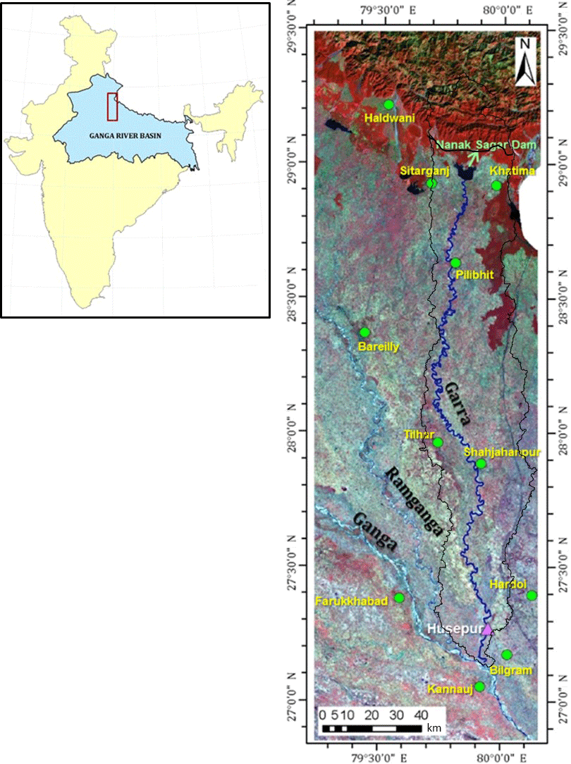
Figure 1 LANDSAT image (1999–2000) in false color composite showing the Garra River basin. The major neighboring rivers (Ganga and Ramganga), location of major cities, the gauging station (Husepur) and the major water structure (Nanak Sagar Dam) are also shown.

2 Study area and data used

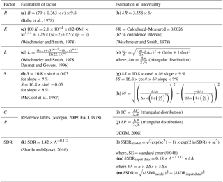
The study basin is the Garra or Deoha River, a Himalayan tributary of the River Ganga. This river originates near Haldwani in Uttarakhand from a lake (29^∘12^′16^′′ N, 79^∘45^′30^′′ E) fed by glacier melt (Roy and Sinha, 2007), and meets the River Ganga near Kannauj in Uttar Pradesh (27^∘08^′30^′′ N, 79^∘56^′40^′′ E). The study basin is located between 27^∘09^′ and 29^∘18^′ N latitude and between 79^∘38^′ and 80^∘09^′ E longitude, covering a total area of around 7000 km² (Fig. 1). The Garra basin has two distinct morphoclimatic regimes, an upper mountainous region (part of Himalayan foothills) and lower alluvial plains (part of the upper Indo-Gangetic Plain). The upper mountainous region of the basin has a high average annual rainfall of 1500 mm, and the lower alluvial part has a comparatively lower average annual rainfall of 1050 mm (Fig. 2d).

Table 1 Data used in the study and their specifications.

The only gauging station in the basin is at Husepur (27^∘16^′30^′′ N, 79^∘57^′0.64^′′ E) near Hardoi, Uttar Pradesh, which was operated by the Central Water Commission (CWC) from 1987 to 2002. The discharge and suspended sediment load records for 16 years (1987–2002) are available at this station. Topography, land use land cover (LULC), soil and rainfall datasets are obtained from different data source agencies listed in Table 1. Table 1 also provides the spatial and temporal resolutions, and temporal extent of these datasets.

The Garra River has a major intervention in the form of Nanak Sagar reservoir (28^∘57^′10^′′ N, 79^∘50^′30^′′ E; capacity 210 Mm³) created by a dam of the same name built in 1962. The reservoir's average sedimentation rate data for the period 1962–2008 (47 years) measured by storage capacity survey are available from a report (CWC, 2015).

3 Methodology

This section describes the methods used for computing SE and SY, and their associated uncertainties. Following the guidelines given by the Joint Committee for Guides in Meteorology (JCGM, 2008), the uncertainties are expressed using standard deviation and reported as percentage of the mean value (coefficient of variation, CV). To combine uncertainties, the general principle of adding uncertainties in quadrature is used (Taylor, 1982). The principle assumes that the individual uncertainties are independent.

3.1 Estimation of soil erosion (SE)

SE is estimated by the revised universal soil loss equation (RUSLE), which is an empirical model for predicting the long-term average rate of SE based on crop system, management techniques and erosion control practices (Renard et al., 1991; Kinnell, 2008). The SE is expressed as a function of five input factors (Eq. 1): rainfall and runoff erosivity (R), soil erodibility (K), slope length and steepness (L and S), cover management (C), and support practice (P) (see Table 2 for their units). These input factors vary considerably from storm to storm, but their effects on the estimation of SE tend to be averaged over extended periods (Wischmeier and Smith, 1978). The methodology for determining the input factors and their uncertainties at each evaluation cell is described below.

$$\begin{array}{}\text{(1)}& \text{SE}=RKLSCP\end{array}$$

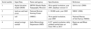
Table 2 Equations and their references for estimating RUSLE factors, sediment erosion and sediment delivery ratio (SDR). Expressions are also given for quantifying and propagating uncertainty based on first-order analysis.

C, the cover and management factor is the ratio of soil loss from an area with specified cover and management to that of an identical area in tilled continuous fallow; ΔC, difference between upper and lower limit of C factor; CV, the coefficient of variation; CS, the coefficient of skewness; Δh, maximum difference in the elevation between the given cell and its neighbor cells (8 neighboring cells in D8 algorithm); δΔh, elevation error in DEM (3.17 m); K, the soil erodibility factor, expressed in the units of t ha hr MJ⁻¹ mm⁻¹ ha⁻¹; L, the slope length factor, is the ratio of soil loss from the field slope length to that from a 22.1 m length under identical conditions; λ, field slope length in meters; δλ, uncertainty in field slope length; M, Particle-size parameter [% silt × (100 – % clay)]; m, variable slope-length exponent (0.3–0.5); δm, uncertainty in variable slope-length exponent; n, number of cells contributing to one cell; OM, organic matter content (%); P, the support practice factor, is the ratio of soil loss with a support practice like contouring, strip cropping, or terracing to that with straight-row farming up and down the slope; p, permeability class (rapid = 1, moderate to rapid = 2, moderate = 3, slow to moderate = 4, slow = 5, very slow = 6); ΔP, difference between the upper and lower limit of P factor; r, the average annual rainfall in mm; R, the rainfall runoff erosivity factor, expressed in the units of MJ mm ha⁻¹ h⁻¹ yr⁻¹; S, the slope steepness factor, is the ratio of soil loss from the field slope gradient to that from a 9 % slope under otherwise identical conditions, sc, soil structure code (very fine granular = 1, fine granular = 2, coarse granular = 3, blocky, platy or massive = 4); SE, the computed soil erosion per unit area expressed in t ha⁻¹ yr⁻¹; SY, the sediment yield at a location in the basin, expressed in t yr⁻¹; θ, slope of the terrain in degrees; Δx, distance between the given cell and the neighboring cell having maximum elevation difference; δΔx, geolocation error in DEM (5.17 m)

3.1.1 Rainfall and runoff erosivity factor (R)

The R factor quantifies the raindrop impact and gives information about the amount and rate of runoff likely to be associated with the rain. The R factor can be obtained by estimating rainfall kinetic energy from rainfall intensity data (Wischmeier and Smith, 1978). As rainfall intensity data are not easily available, empirical equations have been proposed to calculate the R factor from the readily available average annual rainfall data (denoted by r). In this study, we selected the equation proposed by Babu et al. (1978) using the rainfall data from various meteorological stations in India (Eq. 1 in Table 2). Originally, this equation was proposed in “m t cm ha⁻¹ hr⁻¹ year⁻¹” unit by Babu et al. (1978), which needs a multiplication factor of “9.8; to convert into the “MJ mm ha⁻¹ hr⁻¹ year⁻¹” unit (Foster et al., 1981). The uncertainty in the estimate of the R factor arises from model error in the equation of Babu et al. and variability in the observed average annual rainfall (δr). Since model error for the equation of Babu et al. is not available, the uncertainty in R (δR) is estimated solely based on observed rainfall variability (Table 2b).

Figure 2 (a) Elevation (SRTM, 90 m), (b) LULC, (c) soil data from NRSC (2005) and (d) average annual rainfall (1962–2008).

3.1.2 Soil erodibility factor (K)

The K factor represents the susceptibility of soil to erosion due to rainfall and runoff. The K factor is usually obtained from one of the many empirical equations (Wischmeier and Smith, 1978; Declercq and Poesen, 1991; Van der Knijff et al., 2000) that relate it to soil properties like organic matter percentage, soil texture and soil permeability. However, stoniness can also be an important factor to consider while evaluating the K factor (Panagos et al., 2014). The Garra basin has primarily three kinds of soil textures: loam, sand and sandy loam (Fig. 2c) with a negligible amount of gravels. Hence, stoniness is not accounted for in the estimates of the K factor. Therefore, the equation proposed by Wischmeier and Smith (1978, Table 2c) is used for estimating the K factor because all the required input parameters for this equation are available for the study basin. The uncertainty in the K factor can be due to uncertainty in the measurement of soil properties and uncertainty in the model that relates soil properties to the K factor. Since the measurement uncertainties of soil properties are not available for the study basin, only the model uncertainties as given by Wischmeier and Smith (1978) are considered (Table 2).

3.1.3 Slope-length factor (L) and slope steepness factor (S)

The L and S factors represent the effect of topography on SE. They are usually presented as a single factor (LS factor) that represents the ratio of soil erosion for the given conditions to the soil erosion from an experimental plot of slope length 22.13 m and slope steepness 9 %. This study employs the method proposed by Desmet and Govers (1996) for determining the L factor (Table 2d). The method calculates the L factor by considering flow accumulation at each cell obtained from the DEM. The S factor depends only on the local slope. Many empirical equations are available for estimating the S factor (Wischmeier and Smith, 1978; McCool et al., 1987; Moore and Wilson, 1992; Nearing, 1997). Here, the equation proposed by McCool et al. (1987) is adopted because of its popularity and versatility (Table 2f).

Monte Carlo simulations are usually employed for quantifying uncertainties in the LS factor (Biesemans et al, 2000; Catari, 2010; and Tetzlaff et al., 2013). In this method, multiple realizations of the DEM are generated based on a pre-specified error rate in the DEM elevation, and LS factor is calculated for every realization. The variability in LS factors over multiple realizations provides a measure of uncertainty in the LS factor arising due to uncertainties in DEM. The DEM errors are sometimes modeled as an auto-correlated random field (Biesemans et al, 2000); however, in absence of information about the spatial structure of the DEM errors, they are either modeled as independent errors (Tetzlaff et al., 2013) or some simplified assumptions are made on their spatial structure using spatial filters (Catari, 2010). The assumption of independent errors gives the worst-case scenario of DEM uncertainty effects (Wechsler and Kroll, 2006). The Monte Carlo simulations are effective for small-sized basins but become tedious for large basins (Tetzlaff and Wendland, 2012). This study uses the information on geolocation error (δΔx) and elevation error (δΔh) available for the DEM, and applies first-order uncertainty analysis to estimate uncertainties in L (δL) and S (δS) factors (Table 2e, g). The method assumes that the DEM errors are uniform in space and are independent.

The uncertainty in the L factor also depends on the uncertainty in specifying the value of the variable slope exponent (m). The m factor depends on the rill and inter-rill erosion ratio (β). In this study, β is estimated by the equation proposed by McCool et al. (1997). Here, the uncertainty in “m” is modeled as a Type B (assumed probability distribution function based on comparatively reliable information; JCGM, 2008) standard uncertainty assuming a symmetric triangular distribution (JCGM, 2008, pages 11 to 18) over the range of values (0.05–0.25). The combined uncertainty in LS factor (δLS) is obtained by adding δL and δS in quadrature.

Table 3 The C factor for different land use land cover (LULC) classes along with their uncertainties.

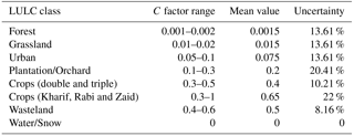
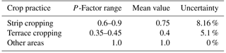
Table 4 Different cropping practice (P) factors for various cropping practices along with their uncertainties.

3.1.4 Cover and management (C) and support practice factor (P)

The C factor is the ratio of soil loss from a given land use class to the corresponding loss from an experimental plot having “clean-tilled and continuous fallow” land use condition. The P factor is the ratio of soil loss from a land with given support practice to the corresponding loss from an experimental plot having an agricultural practice of “upslope and downslope tillage.” The C and P factors for a cell are obtained from reference tables (Morgan, 2009; FAO, 1978) that provide a range for given land use and agricultural practices. Reference values of C and P factors for the classes of land use and agricultural practices considered in this study are given in Tables 3 and 4, respectively. Since the RUSLE is not applicable for glacial erosion and channel processes, the C factor for snow and water-covered cells is taken as zero. The vegetation density obtained using remote sensing (Normalized Difference Vegetation Index) can provide an alternative method to quantify the C factor and its uncertainty.

For an agriculturally dominated basin, the C factor varies seasonally depending upon the cropping cycle. The seasonality in the C factor is incorporated in RUSLE by taking a weighted average of C values during different seasons, where weights are proportional to the R factor (Vanoni, 1975). The study basin has two types of cropping patterns (1) a double and triple cropping pattern in which crops are grown almost all year round and (2) a single cropping (Rabi, Kharif or Zaid) system in which the crops are grown only for a season. Since the farms with a single cropping pattern are fallow during the non-growing season they are attributed with a wider range of C factors (0.3–1) compared to the farms with double and triple cropping patterns (0.3–0.5).

During field visits, we observed that terrace cropping and strip cropping are practiced in most of the upper mountainous region and lower alluvial plains, respectively. For calculating SE, it is assumed that the upper mountainous region has only the terrace cropping practice and lower alluvial plains have only strip cropping practices. The uncertainty in C (δC) and P (δP) factors are obtained by a Type B evaluation of standard uncertainty, assuming a symmetric triangular distribution over the range of values in a given class of land use and agricultural practices (JCGM, 2008), presented in Table 2i, j. The combined effect of land use and land cover is represented by the CP factor, which is a product of C and P factors. The uncertainty in CP factor (δCP) is calculated by adding δC and δP in quadrature.

Finally, assuming that uncertainties in individual factors are independent, they are added in quadrature to calculate relative uncertainty in the estimate of SE for each cell as

$$\begin{array}{}\text{(2)}& {\displaystyle \frac{\mathit{\delta }\text{SE}}{\text{SE}}}=\sqrt{{\left({\displaystyle \frac{\mathit{\delta }R}{R}}\right)}^{\mathrm{2}}+{\left({\displaystyle \frac{\mathit{\delta }K}{K}}\right)}^{\mathrm{2}}+{\left({\displaystyle \frac{\mathit{\delta }\text{LS}}{\text{LS}}}\right)}^{\mathrm{2}}+{\left({\displaystyle \frac{\mathit{\delta }\text{CP}}{\text{CP}}}\right)}^{\mathrm{2}}}.\end{array}$$

3.2 Estimation of the sediment delivery ratio (SDR)

The SDR is defined as the ratio of SY at a prediction location to the gross or total SE of a basin. It is estimated by the empirical equation developed by Sharda and Ojasvi (2016) based on reservoir sedimentation (CWC, 2015) and soil erosion data (Sharda, 2009; NAAS, 2010) from 16 large reservoir basins (basin area greater than 1000 km²) located in north India (Eq. 3).

$$\begin{array}{}\text{(3)}& \text{SDR}=\mathrm{1.817}\times {\mathrm{A}}^{-\mathrm{0.132}}\end{array}$$

For derivation of the above equation, soil erosion rates for India were estimated by employing the RUSLE, but with inconsistent unit system for R and K factors (Maji, 2007; NAAS, 2010). After applying the correction, the SDR values decrease by a factor of 1.28. The corrected equation is

$$\begin{array}{}\text{(4)}& \text{SDR}=\mathrm{1.42}\times {\mathrm{A}}^{-\mathrm{0.132}}\end{array}$$

The equation was fitted by the ordinary least squares method in the logarithmic domain. An expression for uncertainty in SDR prediction (δ SDR) that accounts for model error (δ SDR_model) and uncertainty in the calculation of basin area (δ SDR_input data) derived by using the first-order uncertainty analysis is given in Table 2n.

3.3 Computation of sediment yield (SY)

The SY at a location is estimated by multiplying annual average gross SE and SDR of a drainage basin whose outlet is the estimation point. The uncertainty in SY is computed as the standard deviation of the SY distribution obtained by 1000 Monte Carlo simulations for which gross SE and SDR are simulated using the following distributions:

The gross SE is the sum of average annual SE at all cells in the basin. Assuming the weak form of the central limit theorem to be applicable (i.e., probability distribution of annual average SE at all cells in the basin are non-independent and non-identical), the gross erosion is considered to have a normal distribution with mean and variance equal to the sum of means and variances of SE at individual cells, respectively. A truncated version of the normal distribution in the range [0, ∞) is used to avoid negative values of gross SE during Monte Carlo simulations.

The SDR of the basin is assumed to follow a lognormal distribution with mean and standard deviation given in Table 2k and n, respectively.

In addition to Monte Carlo simulations, uncertainty in SY is also estimated by the first-order uncertainty analysis.

To account for the effect of a dam on SY, we used the method proposed by Sharda and Ojasvi (2016) which assumes that a sufficiently large dam on a river (termed terminal dam) entraps all the sediment carried by the river into its reservoir. Therefore, the gross SE at a location downstream of a terminal dam is estimated from “free basin area” (total basin area minus reservoir catchment area) instead of total basin area. The SY is then calculated as the product of gross SE from the free basin area and SDR of the entire basin.

In this study, annual average SY is estimated at two locations – the Nanak Sagar Dam for the period 1962–2008 and Husepur gauging station for the period 1987–2002. The Nanak Sagar Dam, which lies upstream of the Husepur station, is treated as a terminal dam.

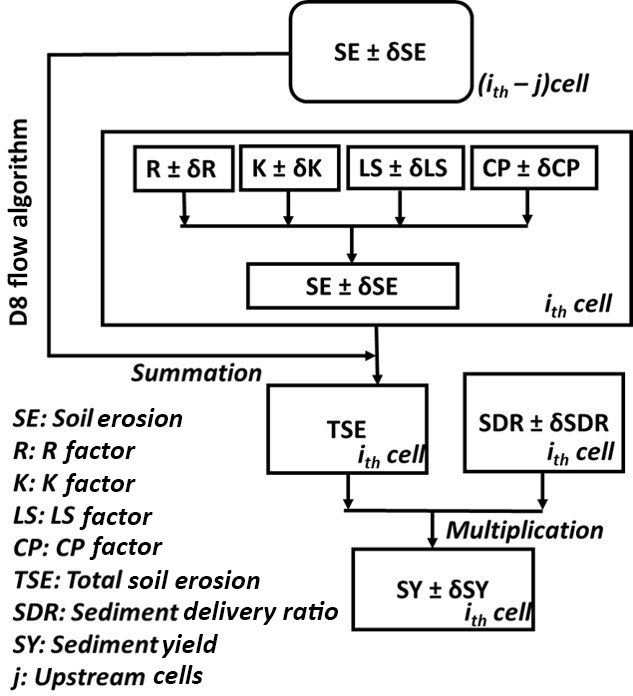
Figure 3 Approach to estimate soil erosion (SE) and sediment yield (SY) with associated uncertainties.

The following steps are followed to estimate the values and corresponding uncertainties in SE, SDR and SY (also shown as a flow chart in Fig. 3):

• The Garra River basin boundary is derived from SRTM data based on the D8 flow direction algorithm (O'Callaghan and Mark, 1984). Hydrological correction of DEM is done by filling of pits in topography (Tarboton et al., 1991). Flow accumulation, flow direction, drainage network and local slope are calculated from the corrected the DEM of the Garra River basin.

• The R, K, L, S, C and P factors and their uncertainties are calculated by using the equations given in Table 2 and explained in the previous sections.

• Spatially distributed SE averaged over the study period is estimated by applying the RUSLE. The uncertainties in individual factors of RUSLE are propagated by first-order uncertainty analysis (Table 2 and Eq. 2) to calculate uncertainty in the estimated SE at each cell. Monte Carlo simulations are used to predict the distribution of SE.

• Mean and variance in gross SE for a basin is estimated by summing up mean and variance in SE at all cells in the basin.

• SDR for a basin is modeled as a lognormal distribution with mean and standard deviation estimated in Table 2k and n, respectively.

• SY at the Nanak Sagar Dam (NSD) and Husepur gauging station (HGS) are estimated by Mote Carlo simulations. Hence 1000 values of gross SE (normal distribution) and SDR (lognormal distribution) are generated and multiplied with each other to simulate 1000 values of SY. The uncertainty in the SY prediction interval is reported as the standard deviation of the simulated SY values.

• The estimated annual average SY at NSD (1962–2008) and HGS (1987–2002) are compared with observed values to assess the suitability of the proposed methodology.

4 Results and discussion

4.1 Soil erosion (SE)

First, the results of RUSLE factors are presented, which are followed by the results of SE estimation. The results presented are the average value during the entire study period (1962–2008).

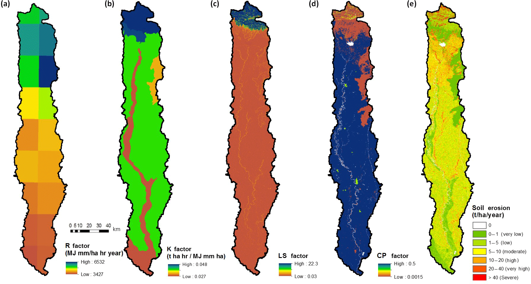
Figure 4 (a) Rainfall runoff erosivity (R), (b) soil erodibility (K), (c) topographic steepness (LS), (d) crop practice (CP) factors and (e) soil erosion estimation for the Garra River basin.

4.1.1 R factor

The R factor (Fig. 4a) follows the same spatial pattern as average annual rainfall (Fig. 2d) – high in the upper mountainous region where average annual rainfall exceeds 1000 mm. The factor gradually reduces in the lower alluvial parts and attains the minimum values near the basin outlet. The uncertainty in R factor that stems from variability in annual rainfall varies in a relatively narrow range of 3.4 to 6.7 % (Fig. 5a).

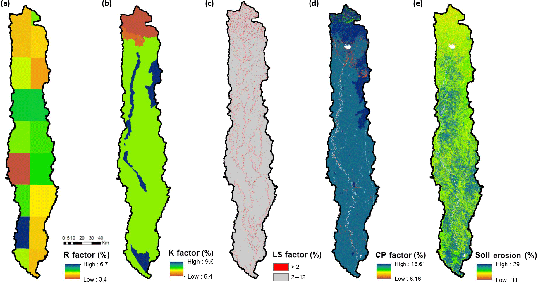
Figure 5 Percentage uncertainty in (a) rainfall erosivity, (b) soil erodibility, (c) topographic steepness, (d) crop and practice, and (e) soil erosion uncertainty in percentage for the Garra River basin.

4.1.2 K factor

The soil map (Fig. 2c) shows the presence of sand and sandy loam soil close to the main channel and in forested patches of the basin; the rest of the basin is covered primarily with loam. Typically, the loam is more susceptible to erosion than sand and sandy loam, which is reflected in higher values of the K factor (Fig. 4b). The upper mountainous region shows highest values of K factor because the loam in this region has a higher silt content (∼40 %) compared to loam in lower alluvial plains (∼30 %). The magnitude of model uncertainty in δK is constant for the basin, hence the percentage uncertainty is lower for cells with larger K factor (upper mountainous region) than for cells along the main channel that have a low value of the K factor. The uncertainty varies from 5.4 to 9.6 % (Fig. 5b).

4.1.3 LS factor

The LS factor shows considerable variation, particularly in the upper mountainous region where its value ranges from 5 to 22.3 (Fig. 4c). The larger values and higher variation in the upper mountainous region can be attributed to the steeper slopes (S factor) and its varying topography. The LS factor is also relatively high for cells close to the stream mainly because of the large contributing area (L factor). For the rest of the basin, the LS factor is small (<1) and shows little variability. The uncertainty in LS factor also shows a considerable variation. The magnitude of uncertainty is significant for cells near the channel and upper mountainous region. However, these cells have least percentage uncertainty (<2 %) because of the higher magnitude of the LS factor (Fig. 5c). The percentage uncertainty in the rest of the basin varies between 2 and 12 % (Fig. 5c).

4.1.4 CP factor

The spatial map of CP factor (Fig. 4d) resembles distinct land use land cover (LULC) features present in the basin. The factor is 0 for snow and water covered cells. It attains a low value (<0.1) for forested cells (16 % of basin area), intermediate values (0.2–0.3) for urban cells (0.4 % of basin area) and highest values (>0.4) for cropland cells (71 % of basin area). The uncertainty in CP factor also varies according to LULC type and crop practice class as shown in Tables 3 and 4. The percentage uncertainty varies from 8.2 to 13.6 % (Fig. 5d).

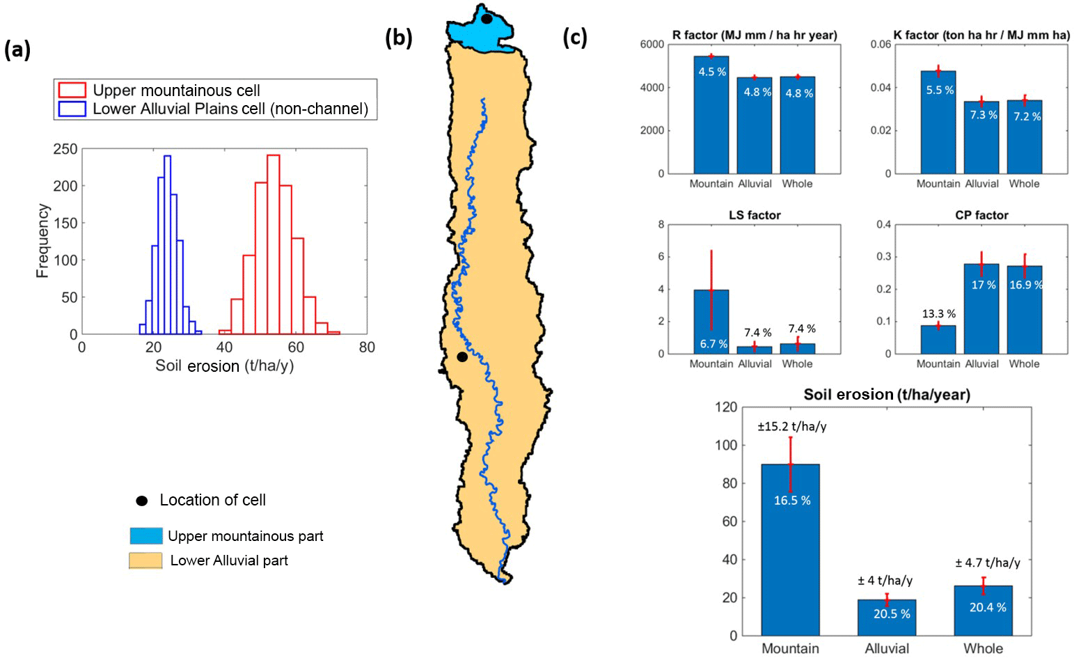
Figure 6 (a) Distribution of SE at their representative cells in the basin, namely upper mountainous part and lower alluvial part. (b) Upper mountainous and alluvial plains parts of the basin. (c) Comparison between the different factors of RUSLE and SE for both region.

4.1.5 Soil erosion (SE)

Finally, results of all the factors described in the preceding subsection are combined by using Eqs. (1) and (2) to obtain the SE map (Fig. 4e) and its uncertainty (5e), respectively. Two distinct geomorphic settings in the basin – the upper mountainous region and the lower alluvial plains – show significant differences in SE. The factors governing the rate of SE in these two settings are compared in Figs. 6 and 7. The SE is the highest in the upper mountainous region (SE > 40 t ha⁻¹ yr⁻¹; severe category). For the cells near the channels, the rate of erosion falls in the zone of very high (20 to 40 t ha⁻¹ yr⁻¹) and severe (>40 t ha⁻¹ yr⁻¹) categories. Other parts of the basin have a moderate (<10 t ha⁻¹ yr⁻¹) to high (10–20 t ha⁻¹ yr⁻¹) SE rate. The average rate of SE for the entire Garra basin is 23 t ha⁻¹ yr⁻¹ (very high), whereas for the upper mountainous region and lower alluvial plains the values are 92 t ha⁻¹ yr⁻¹ (severe) and 19.3 t ha⁻¹ yr⁻¹ (high), respectively.

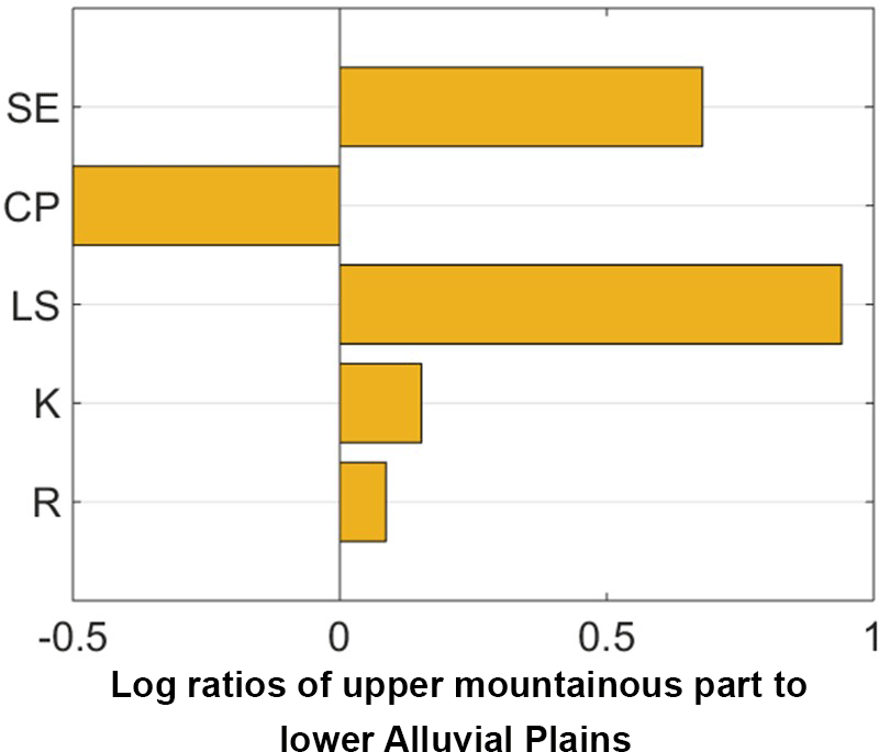
Figure 7 Comparison of RUSLE factors (R, K, LS and CP) and SE rates (SE) for upper mountainous and lower alluvial plains in the study basin.

The upper mountainous region has higher values of R, K and LS factors than the lower alluvial plains. A significant portion of the alluvial plains has cultivated land where the agricultural practices tend to make the soil more susceptible to sheet erosion during rainfall. Hence, the CP factor is higher for the alluvial plains. Nevertheless, the higher erosion rates in the mountainous region can be attributed mainly to the higher values of LS factor due to steeper slopes.

The uncertainty map of SE rate (Fig. 5e) reflects the spatial distribution of uncertainty in individual factors. The uncertainty tends to be high for sandy loam and sandy soil patches in the basin. The percentage uncertainty in the upper mountainous region is lower (16.5 %) than that for the alluvial plains (20.5 %). However, uncertainties in the magnitude of erosion rate are higher for the mountainous region (15.2 t ha⁻¹ yr⁻¹) than for the alluvial plains (4 t ha⁻¹ yr⁻¹). The magnitude and percentage uncertainty in RUSLE factors and SE rate averaged over the entire basin is very similar to that of the alluvial plains that constitute a major portion of the basin (95 %; Fig. 6b).

Table 5 Comparison of uncertainties in RUSLE factors and soil erosion (SE) reported in the literature and those obtained in the present study. The present study employs forward uncertainty propagation for the Garra river basin.

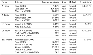
Figure 6a shows the distribution of SE at two representative cells in the upper mountainous region and lower alluvial plains obtained by the Monte Carlo simulations. The cell in the mountainous region has a higher value of SE and its distribution has a wider spread compared to that of the cell in the alluvial plains. Both distributions are positively skewed, although the magnitude of the coefficient of skewness is small (0.11 for mountainous regions and 0.13 for alluvial plains). Table 5 compares the uncertainties in RUSLE factors and SE reported in the literature, and those obtained in the present study. The reported uncertainties in SE have a wide range that encompasses the uncertainty range estimated in the present study. The backward uncertainly propagation method uses observed data and thus represents true uncertainty. The forward method gives an approximation of the true uncertainty, and usually under-predicts the true value.

4.2 Sediment delivery ratio (SDR) and sediment yield (SY)

The SDR and its uncertainty (reported as coefficient of variation in parenthesis) for the Nanak Sagar Dam (NSD) and Husepur gauging station (HSG) are 0.63 (4.40 %) and 0.45 (4.81 %), respectively. For both locations, the SDR model uncertainty component (δ SDR_model) dominates total SDR uncertainty (δSDR_model>0.95 δ SDR). The gross SE at the NSD and HSG sties and its uncertainty are 10.9 × 10⁵ t yr⁻¹ (16.63 %) and 14.9 × 10⁶t yr⁻¹ (20.65 %), respectively. The SY and its uncertainty estimated by the first-order uncertainty analysis at NSD and HSG sites are 6.9 × 10⁵ t yr⁻¹ (17 %) and 6.7 × 10⁶ t yr⁻¹ (21 %), respectively. Figure 8 shows the distribution of SY at the two sites obtained by the Monte Carlo simulations. The distributions at both sites are positively skewed. The standard deviations of the simulated SY at the two sites are almost equal to that obtained from the first-order uncertainty analysis. The SY at NSD and HGS are estimated to be 6.9 ± 1.2 × 10⁵ t yr⁻¹ and 6.7 ± 1.4 × 10⁶ t yr⁻¹, respectively, and the estimated 90 % interval contains the observed values of 6.4 ± 10⁵ t yr⁻¹ and 7.2 × 10⁶ t yr⁻¹, respectively.

5 Limitations

This study presents a methodology for quantifying uncertainty in the estimate of SE and SY for ungauged basins based on the RUSLE-SDR approach. Uncertainties in SE and SY arise from uncertainties in data, model and due to the stochastic nature of the soil erosion process. Like most of the previous studies (referred to in Sect. 1), the proposed methodology accounts for only those sources of uncertainties that are available or could be quantified easily. For example, models or equations used for estimating R and LS do not provide sufficient details to ascertain model uncertainties, hence only data uncertainties are accounted for. On the other hand, uncertainties in data needed for estimating K and CP factors are not available. Hence, only model uncertainties are considered. Thus, the proposed methodology does not account for certain sources of uncertainties leading to under estimation of SE and SY prediction uncertainty. Further, the proposed methodology assumes spatial independence of certain RUSLE factors like R, L, S, C and P factors, resulting in further underestimation of SE and SY prediction uncertainty.

We have demonstrated the proposed methodology by applying it to Garra River basin. The basin has data restrictions that are typical of river basins in India. The spatial distributions of SE and SY for the study basin are obtained by using land use land cover data for 2005, which may not be a true representation of basin conditions during the study period (1962–2008). Further, the study has used gridded daily rainfall data available at a spatial resolution of $\mathrm{0.25}{}^{\circ }\times \mathrm{0.25}{}^{\circ }$ obtained by interpolating rain gauge observations. The coarser spatial resolution of the data is not sufficient to capture the spatial variability of rainfall in the basin. In addition, the gridded rainfall data may have large interpolation errors, which are not accounted for because they are not available for the study basin.

In spite of many limitations, the proposed framework for quantifying and propagating uncertainties in SE and SY appears promising, particularly for ungauged basins in which sheet and rill erosion form the major component of total erosion.

6 Summary and concluding remarks

The main objective of this work is to present a methodology for quantifying uncertainties in the estimates of soil erosion (SE) and sediment yield (SY) at ungauged basins. A systematic procedure is provided for evaluating and propagating uncertainties in a RUSLE-SDR-based approach for SE and SY prediction. Expressions for uncertainty propagation are derived using first-order uncertainty analysis making the proposed methodology viable even for large river basins. The novelty of the work lies in presenting a unified framework for quantifying uncertainties in SE and SY that is applicable to ungauged basins with storage structures. The methodology has been applied on the Garra River basin in India and the major conclusions derived from this study are listed below:

• The SE in the basin is very high (23 ± 4.7 t ha⁻¹ yr⁻¹) with higher values in the upper mountainous region (92 ± 15.2 t ha⁻¹ yr⁻¹) than in the lower alluvial plains (19.3 ± 4 t ha⁻¹ yr⁻¹).

• The LS and CP factors govern the magnitude of soil erosion and its uncertainty in the upper mountainous region and lower alluvial plains, respectively.

• Sediment delivery ratio (SDR) values for Nanak Sagar Dam (NSD) and Husepur gauging station (HSG) are estimated to be 0.63 and 0.45, respectively, with about 5 % uncertainty in both the estimates.

• The SY at NSD and HSG are estimated to be 6.9 × 10⁵ t yr⁻¹ (17 %) and 6.7 × 10⁶ t yr⁻¹ (21 %), respectively. The observed values at the two sites are 6.4 × 10⁵ t yr⁻¹ and 7.2× 10⁶ t yr⁻¹, respectively, and they lie within the estimated 90 % confidence interval. The results suggest that the proposed approach could be effective for sheet or rill erosion-dominated Himalayan river basins like the Garra basin.

The uncertainty in SY derived from Monte Carlo simulations and first-order uncertainty analysis are very similar. The distributions of SY at both sites are positively skewed, although the magnitude of the coefficient of skewness is small. Not all sources of uncertainties could be accounted for in the study because of limited data availability. Hence, the estimated uncertainties in SE and SY are an underestimation of the true uncertainties. A review of uncertainties reported in the literature suggests that true uncertainty can be much higher than the predicted uncertainty. However, in absence of long records of observed SY, the quantification of true uncertainty remains a challenge.