the Creative Commons Attribution 4.0 License.
the Creative Commons Attribution 4.0 License.
 | 23 Mar 2018
Evaluation of ensemble precipitation forecasts generated through post-processing in a Canadian catchment
Sanjeev K. Jha
Durga L. Shrestha
Tricia A. Stadnyk
Paulin Coulibaly
Flooding in Canada is often caused by heavy rainfall during the snowmelt period. Hydrologic forecast centers rely on precipitation forecasts obtained from numerical weather prediction (NWP) models to enforce hydrological models for streamflow forecasting. The uncertainties in raw quantitative precipitation forecasts (QPFs) are enhanced by physiography and orography effects over a diverse landscape, particularly in the western catchments of Canada. A Bayesian post-processing approach called rainfall post-processing (RPP), developed in Australia (Robertson et al., 2013; Shrestha et al., 2015), has been applied to assess its forecast performance in a Canadian catchment. Raw QPFs obtained from two sources, Global Ensemble Forecasting System (GEFS) Reforecast 2 project, from the National Centers for Environmental Prediction, and Global Deterministic Forecast System (GDPS), from Environment and Climate Change Canada, are used in this study. The study period from January 2013 to December 2015 covered a major flood event in Calgary, Alberta, Canada. Post-processed results show that the RPP is able to remove the bias and reduce the errors of both GEFS and GDPS forecasts. Ensembles generated from the RPP reliably quantify the forecast uncertainty.
- Article
(6138 KB) - Full-text XML
-
Supplement
(3207 KB) - BibTeX
- EndNote


Quantitative precipitation forecasts (QPFs) obtained from numerical weather prediction (NWP) models are one of the main inputs to hydrological models when used for streamflow forecasting (Ahmed et al., 2014; Coulibaly, 2003; Cuo et al., 2011; Liu and Coulibaly, 2011). A deterministic forecast, representing a single state of the weather, is unreliable due to known errors associated with the approximate simulation of atmospheric processes and errors in defining initial conditions for a NWP model (Palmer et al., 2005). A single estimate of streamflow using a poor- or high-quality precipitation forecast would have a significant impact on decision support, such as management of water structures, issuing warnings of pending floods or droughts, or scheduling reservoir operations. In recent years, there has been growing interest in moving toward probabilistic forecasts, suitable for estimating the likelihood of occurrence of any future meteorological event, thus allowing water managers and emergency agencies to prepare for the risks involved during low- or high-flow events, at least a few days or weeks in advance (Palmer, 2002). The precipitation forecasts, however, are constrained by major limitations surrounding the technical difficulties and computational requirements involved in perturbing initial conditions and physical parametrization of the NWP model. The QPFs, ensemble or deterministic, have to be post-processed prior to use as reliable estimates of any observations (e.g., streamflow).
In the last decade, several post-processing methods reliant on statistical models have been proposed. The basic idea is to develop a statistical model by exploiting the joint relationship between observations and NWP forecasts, to estimate the model parameters using past data, and to reproduce post-processed ensemble forecasts of the future (Roulin and Vannitsem, 2012; Robertson et al., 2013; Chen et al., 2014; Khajehei, 2015; Shrestha et al., 2015; Khajehei and Moradkhani, 2017; Schaake et al., 2007; Wu et al., 2011; Tao et al., 2014). The range of complexity in the post-processing approaches varies from regression-based approaches to parametric or nonparametric models based on meteorological variables (wind speed, temperature, precipitation etc.) and specific applications. Precipitation is known to have complex spatial structure and behavior (Jha et al., 2015a, b). Thus it is much more difficult to forecast than other atmospheric variables because of nonlinearities and the sensitive processes involved in its generation (Bardossy and Plate, 1992; Jha et al., 2013). From the perspective of a hydrologic forecast center, the post-processing approach should be effective while involving few parameters. For instance, the US National Weather Service River Forecast System has been using an ensemble pre-processing technique that constructs ensemble forecasts through the Bayesian forecasting system by correlating the normal quantile transform of QPFs and observations (Wu et al., 2011). In order to introduce space–time variability of the precipitation forecast in the ensemble, the post-processed forecast ensemble is reordered based on historical data using the Schaake shuffle procedure (Clark et al., 2004; Schaake et al., 2007). This pre-processing technique requires a long historical hindcast database as it relates single NWP forecasts to corresponding observations. In Australia, Robertson et al. (2013) developed a Bayesian post-processing approach called rainfall post-processing (RPP) to generate precipitation ensemble forecasts. The approach was based on combining the Bayesian Joint Probability approach of Wang et al. (2009) and Wang and Robertson (2011) with the Schaake shuffle procedure (Clark et al., 2004). In contrast to the ensemble pre-processing technique, the RPP approach of Robertson et al. (2013) has been described with few parameters and it can better deal with zero value problems in NWP forecasts (Tao et al., 2014) and observations. The RPP approach has been successfully applied to remove rainfall forecast bias and quantify forecast uncertainty from NWP models in Australian catchments (Bennett et al., 2014; Shrestha et al., 2015).
Recent developments in post-processing techniques and the advantage of generating ensembles, and thus estimating uncertainty, are well established in the literature. In an operational context, however, forecast centers in Canada tend to use deterministic forecasts in hydrologic models to obtain streamflow forecasts. The main reasons for this are the higher spatial and temporal resolution of the deterministic forecasts over the ensemble QPFs and the associated computational complexities in dealing with ensemble members. The added advantages of using ensemble forecasts over deterministic forecasts have been addressed in many previous studies (e.g., Abaza et al., 2013; Boucher et al., 2011). When the computational facilities are available, using a set of QPFs obtained from different NWP models run by different agencies (such as the European Centre for Medium-Range Weather Forecasts, the Japan Meteorological Agency, the National Center for Environmental Prediction (NCEP), the Canadian Meteorological Center) seems to be a preferred choice (Ye et al., 2016; Zsótér et al., 2016; Qu et al., 2017; Hamill, 2012).
The main hypothesis we want to test in this study is whether the RPP approach can be directly applied to Canadian catchments or any modification is required. Based on this hypothesis, the aims of this study are to (a) evaluate the performance of RPP in improving cold regions' precipitation forecasts; (b) compare the ensembles generated from applying RPP to the deterministic QPFs obtained from the Global Ensemble Forecasting System (GEFS) and the Global Deterministic Forecast System (GDPS) (referred to as calibrated QPFs); and (c) investigate forecast performance during an extreme precipitation event like that of 2013 in Alberta, Canada. The methodology and description of the study area and datasets are presented in Sect. 2. Section 3 presents methodology, followed by results in Sect. 4 and discussion and conclusion in Sect. 5.

Although the current study uses the RPP approach previously published in Robertson et al. (2013) and Shrestha et al. (2015), there are many novel aspects of this study, which are listed below.
- i.
Robertson et al. (2013) demonstrated the application of the RPP approach at rain gauge locations in a catchment in southern Australia. In the present study, we are applying RPP at the subcatchment level using subcatchment-averaged forecasts and observations, which is similar to the work presented in Shrestha et al. (2015).
- ii.
The physiography and orography effects over western catchments of Canada significantly differ from the Australian catchments considered in Shrestha et al. (2015). In their analysis, Shrestha et al. (2013) considered 10 catchments in tropical, subtropical, and temperate climate zones with catchment areas ranging from 87 to 19 168 km2 distributed in different parts of Australia. Each catchment was further divided into smaller subcatchments and RPP was applied in each of them. In the present study, we focus on only a specific region of Canada with a cold and snowy climate, consisting of 15 subcatchments with areas ranging from 734 to 2884 km2. We apply RPP to each subcatchment using the forecast and observation data lying within it. The size of the subcatchment plays an important role in estimating the subcatchment-averaged forecast and observations.
- iii.
The results from different NWP models are known to vary due to approximations involved in the simulation of atmospheric processes and applied initial and boundary conditions, etc. In the present study, we used two precipitation forecasts obtained from the Global Ensemble Forecast System (GEFS) Reforecast Version 2 data, from the National Centers for Environmental Prediction, and the Global Deterministic Forecast System (GDPS), from Environment and Climate Change Canada (ECCC). Shrestha et al. (2013) used forecasts from only one NWP model, the Australian Community Climate and Earth-System Simulator. Further, we compare the performance of RPP applied to GEFS and GDPS forecasts in order to decide which forecast is best suited to our study area.
- iv.
Although QPFs from the GDPS are routinely used at the forecast centers in Canada, the application of GEFS to catchments in western Canada is not known, to the best of our knowledge (also confirmed from data provider, Gary Bates at NOAA, personal communication, 21 March 2017).
- v.
In their analysis, Shrestha et al. (2013) considered 3-hourly forecasts for 615 days only. In the current study, 3 years of daily forecasts are used without any gap. The longer data record is recommended as it can help in inferring the parameters of RPP more accurately.
- vi.
In the present study, we explicitly look at an extreme precipitation event that happened in Calgary 2013 and evaluate the performance of the RPP approach in generating ensembles, which was not done in previous works (Shrestha et al., 2015; Robertson et al., 2013).
- vii.
To the best of our knowledge, this is the first time an approach for generating ensembles from a deterministic QPF is tested in any Canadian catchment explicitly for the benefit of forecast centers. As part of the National Sciences and Engineering Research Council Canadian Floodnet 3.1 project, the first author visited flood forecast centers in western Canada. One of the common concerns raised by forecasters was the need for generating ensembles in order to assess risk associated with streamflow forecasts provided to the public. The conclusions from the present study will be highly relevant and beneficial for flood forecast centers in Canada.
The selected study area is southern Alberta, located in western Canada (Fig. 1a). The Rocky Mountains are located at the southern boundary with the United States and the western boundary with British Columbia, with the Canadian Prairies region extending toward the southeastern portion of the province. Topography plays a major role in generating cyclonic weather systems common to Alberta. The Oldman, Bow, and Red Deer River basins, all located at the foothills of the Canadian Rocky Mountain range, are subjected to extreme precipitation events. In June 2013 a major flood occurred in this region, resulting from the combined effect of heavy rainfall during mountain snowpack melt over partially frozen ground (Pomeroy et al., 2016; Teufel et al., 2016). Some river basins received -year rainfall, estimated to be 250 mm rain in 24 h. The 2013 flood affected most of southern Alberta from Canmore to Calgary and beyond, causing evacuation of around 100 000 people and a reported cost of damage of infrastructure exceeding CAD 6 billion (Milrad et al., 2015). The spatial distribution of convective precipitation and orography make it difficult for any NWP model to successfully predict the summertime convective precipitation in Alberta. The NWP forecasts at the time predicted less (about half of the actual amount) rainfall during this event (AMEC, 2014).
The dataset used in this study consists of observed and forecast daily precipitation over the period of 2013 to 2015, including the heavy precipitation event causing the major flood of 2013. Observed data were obtained from the Environment and Climate Change Canada precipitation gauges. Two precipitation forecasts, GEFS and GDPS, were obtained from National Centers for Environmental Prediction and Environment and Climate Change Canada respectively. A description of both forecasts is presented in Table 1. The spatial resolution of GEFS forecasts is 0.47∘ latitude, 0.47∘ longitude. GEFS contains 11 forecast members including one control run and 10 ensembles. The control run uses the same model physics but without perturbing the analysis or model. The ensembles are obtained by perturbing the initial conditions slightly (WMO, 2012). The forecast is available at 00:00 UTC at an interval of 3 h for the first 3 days and then 6-hourly up to 8 days. It is worth pointing out here that in the GEFS data, the forecasts at hours 3, 9, 15, and 21 are 3 h accumulations, whereas the forecasts at 6, 12, 18, and 24 h are 6 h accumulations for forecasts valid for days 1 to 3. In order to obtain a 24 h (daily) forecast for days 1, 2, and 3, we need to consider the summation of forecasts valid at hours 6, 12, 18, and 24 for a given day. For days 4 and 5, forecasts are only available for 6, 12, 18, and 24 h (i.e., there is no forecast for the 3 h accumulation). The control run of GEFS for a period of 3 years (1 January 2013 to 31 December 2015) with a lead time of 5 days is used in the present analysis.
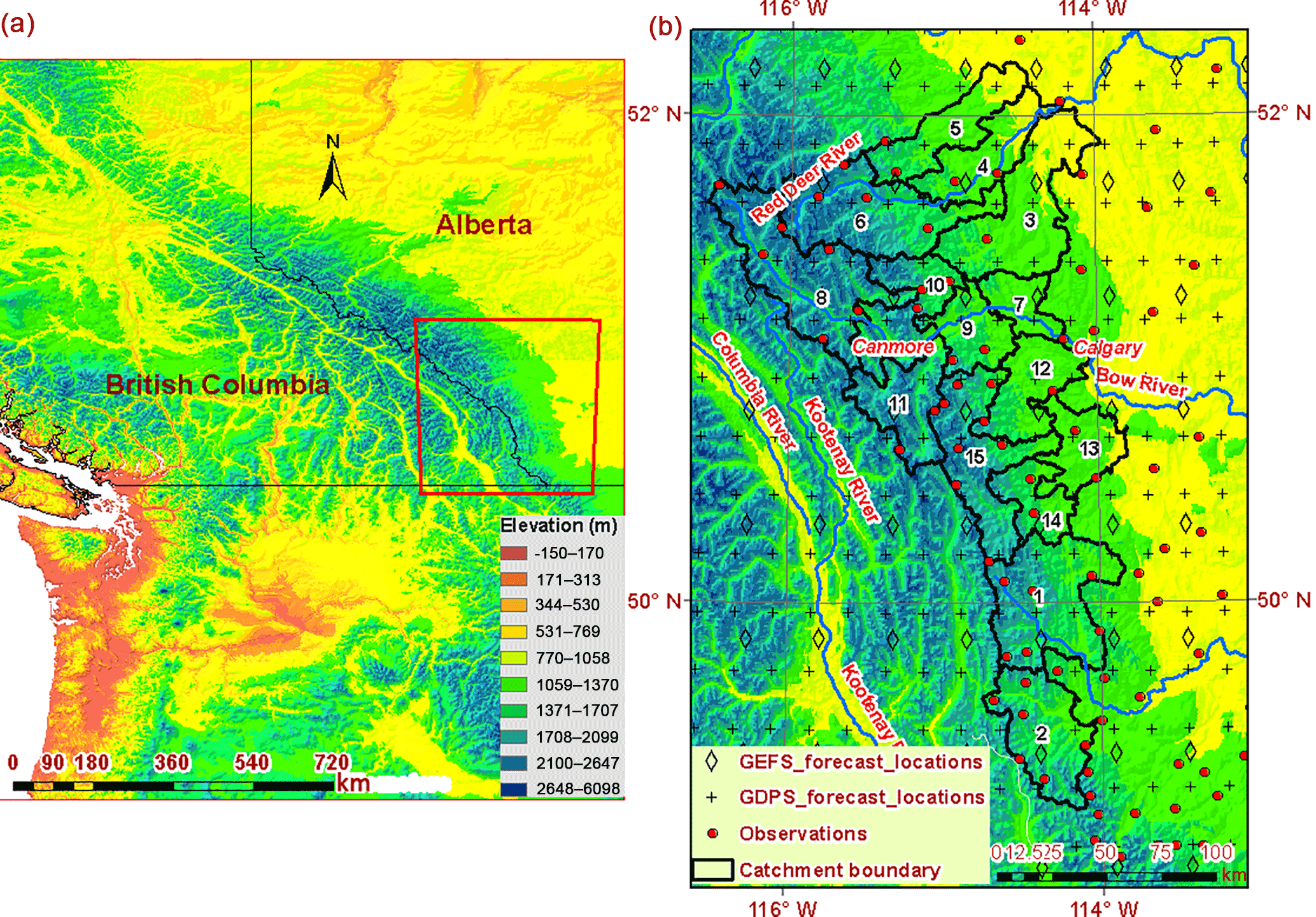
Figure 1Location of the study basin in Alberta, Canada, showing (a) topography, a major driver of different precipitation mechanisms, and (b) the study area with locations of observed and forecast data.
GDPS precipitation forecasts are obtained from the Canadian NWP model, the Global Environmental Multiscale Model. The forecasts are available at approximately 0.24∘ latitude, 0.24∘ longitude spatial resolution at an interval of 3 h for forecast lead times up to and beyond 2 weeks. Precipitation forecasts are accumulations from the start of the forecast period. To obtain a forecast for a specific day, for example day 2, the precipitation forecast at the end of day 1 has to be subtracted from the precipitation forecast at the end of day 2. Three years of continuous GDPS forecasts from 1 January 2013 to 31 December 2015 with lead times of 5 days at 00:00 UTC are used in the present analysis.
There are three major rivers passing through the study area: Bow, Oldman, and Red Deer rivers (Fig. 1b). Based on the world map of Peel et al. (2007), the study area is classified as having a warm summer, humid continental climate. The Köppen–Geiger classification system presented for Canada in Delavau et al. (2015) shows that our study area falls within the KPN42 (Dfb – snow, fully humid precipitation, warm summer), KPN43 (Dfc – snow, fully humid precipitation, cool summer), and KPN 62 (ET polar tundra). All of the three river basins are part of the South Saskatchewan River basin, which flows eastward towards the Canadian Prairies. The combined basin area is approximately 101 720 km2 (AEP, 2017). For the purpose of hydrological prediction, the River Forecast Centre in Alberta uses 15 subcatchments (marked with numbers 1 to 15 in Fig. 1b) to delineate the study area, with drainage areas as indicated in Table 2.
Table 2Description of subcatchments in the study area. Italics is used to highlight maximum and minimum values in the corresponding columm.
The distribution of precipitation gauges and forecast locations is uneven in the various subcatchments (Fig. 1b). For hydrological modeling purposes, average precipitation over each subcatchment is calculated using an inverse-distance weighting method (Shepard, 1968), considering four neighboring gauges. Subcatchment 2 receives the highest subcatchment-averaged annual precipitation, while subcatchment 13 receives the lowest average annual precipitation during the 3-year study period (Table 2). In each subcatchment, an area-weighted forecast is calculated by considering the portion of the forecast grid that overlaps with the subcatchment.
Figure 2 shows the comparison of raw QPFs and observed precipitation in subcatchments 10 and 11 for GEFS and GDPS with a lead time of 1 day for 2013. The large peak observed (Fig. 2a–d) is the result of a major rainfall event responsible for severe flooding in Alberta in June 2013. Figure 2 indicates that there is a substantial bias between the raw QPFs and observations. Raw QPFs from GEFS and GDPS consistently underestimate peak events and medium precipitation amounts, which is of concern to hydrologic forecast centers predicting streamflow peak volume and timing.

Figure 2Comparison of weighted-area raw QPFs with subcatchment-averaged observations for the year 2013 in subcatchments 10 and 11. Raw GEFS data are plotted in (a) and (b), while (c) and (d) show raw GDPS data, along with observations.
3.1 Post-processing approach
We use the RPP to post-process the precipitation forecasts. The RPP was developed by Robertson et al. (2013) and successfully applied to a range of Australian catchments (Shrestha et al., 2015). Detailed descriptions of the RPP can be found in the above references; here we present a brief overview of the method.
The input to the post processing approach is observations (zo) and raw QPFs (zrf). A log-sinh transformation is applied to both observations and raw precipitation forecasts:
where and are transformed observation and raw forecasts; αo and βo are parameters used in the transformation of zo; and αf and βf are parameters used in the transformation of zrf. It is assumed that the transformed variables ( and follow a bivariate normal distribution , in which μ and Σ are defined as follows:
where and represent the mean and standard deviation of respectively; and represent the mean and standard deviation of respectively; is the correlation coefficient between and . Thus, there are nine parameters (αo, βo, , , αf, βf, , , ) to model the joint distribution of raw QPFs and observations. We infer a single set of model parameters that maximizes the likelihood of posterior parameter distribution using the shuffled complex evolution algorithm (Duan et al., 1994). All model parameters are reparametrized to ease the parameter inference. Once the parameters are inferred, the forecast is estimated using the bivariate normal distribution conditioned on the raw forecast. The random sampling from the conditional distribution generates the ensemble of forecasts. The forecast values are then transformed to the original space using the inverse of Eqs. (1) and (2).
Since the forecasts are generated at each location for each lead time separately, the space–time correlation in the ensemble members will be unrealistic. The Schaake shuffle (Clark et al., 2004) is then applied to adjust the space–time correlations in the ensemble, similar to what was observed in the historically observed data. The Schaake shuffle calculates the rank in the observed data and preserves the same rank in the sorted, new ensemble forecast. Our application of the Schaake shuffle is briefly described here.
- 1.
For a given forecast date, an observation sample (date and amount of data) of the same size as that of the ensemble is selected from the historical observation period.
- 2.
The observation sample data for each lead time are ranked. Similarly, the data from the forecast ensemble for each lead time are ranked.
- 3.
A date from the observation sample is randomly selected and the ranks of the observation data for the selected date for all lead times are identified.
- 4.
For a given lead time, we select the forecast (from the forecast ensemble) that has the same rank as that of the selected observation.
- 5.
In order to construct an ensemble trace across all lead times, step 3 is repeated for all lead times.
- 6.
Steps 3 to 5 are repeated as many times as the size of ensembles.
The above procedure is extended for both temporal and spatial correlation in this study.
An important feature of the RPP is the treatment of (near) zero precipitation values, which are treated as censored data in the parameter inference. This enables the use of the continuous bivariate normal distribution for a problem, which is otherwise solved using a mixed discrete–continuous probability distribution (e.g., Wu et al., 2011).
3.2 Verification of the post-processed forecasts
We assess the processed forecast in terms of deterministic metrics, such as percent bias defined as percent deviation from the observations (bias, %), mean absolute error (MAE in mm), and a probabilistic metric, a continuous rank probability score (CRPS), at each site for the forecast period (t). The percent bias is estimated as follows:
where zf could either be raw (zrf) or post-processed forecasts (zpf), and zo represents observation.
MAE measures the closeness of the forecasts and observations over the forecast period.
In the case of the ensemble forecast, we use the mean value of forecasts in the calculation of both the bias and the MAE. A low value of both bias and MAE indicates that the forecasts are closer to observations. A percent bias close to zero indicates that forecasts are unbiased.
The CRPS is a probabilistic measure to relate the cumulative distribution of the forecasts and the observations:
where is the cumulative distribution function of ensemble forecasts and is the cumulative distribution function of observations, which turns out to be a Heaviside function (1 for values greater than the observed value, otherwise 0). In the case of the deterministic forecast, the CRPS reduces to the MAE. The forecast is considered better when the CRPS values are close to zero.
The relative operating characteristic (ROC) curves are used to assess the forecast's ability to discriminate precipitation events in terms of hit rate and false alarm rate. Given a precipitation threshold, the hit rate refers to the probability of forecasts that detected events smaller or larger in magnitude than the threshold; the false alarm rate refers to the probability of erroneous forecasts or false detection (Atger, 2004; Golding, 2000). If the ROC curves (plot between hit rate versus false alarm rate) approach the top left corner of the plot, the forecast is considered to have a greater ability to discriminate precipitation events. The discrimination ability of the forecast is considered low when the ROC curves are close to the diagonal.
To compare the spread in forecast ensembles against the observations, we perform spread–skill analysis by plotting the ensemble spread versus the forecast error (e.g., Nester et al., 2012). The ensemble spread is defined as the mean absolute difference between the ensemble members and the mean. The absolute difference between the observations and the ensemble mean is defined as the forecast error. For each lead time in the cross-validation period, we compute the ensemble spread and forecast error for 1000 ensemble forecasts, sort them in increasing order, group the values in 10 classes, and calculate the average spread and error in each class.
3.3 Statistical treatment of forecasts
Because of the short record of data (3 years only), few extreme events may significantly affect the verification scores. Therefore it is desirable to understand the effect of the sampling variability on the verification scores. Accounting for sampling variability in calculating the verification scores adds confidence that results are robust and likely to apply under operational conditions (Shrestha et al., 2015). We calculate sampling uncertainty through a bootstrap procedure (e.g., Shrestha et al., 2013). The first 1095 pairs (3 years of data) of forecast–observations are sampled with replacement from the original forecast–observation pairs, with replacement and verification scores calculated (discussed in Sect. 3.1 below). These steps are repeated 5000 times to obtain a distribution of the verification score, from which 5 and 95 % confidence intervals are calculated.
3.4 Experimental setup
Post-processing is applied to precipitation forecasts in 15 subcatchments, making use of the subcatchment-averaged precipitation forecast data for the total study duration (i.e., 2013 to 2015 for GEFS and GDPS), for each day of forecast at 00:00 UTC up to a lead time of 5 days. We apply a leave-1-month-out cross-validation approach. The simulation runs in two modes: inference and forecast. In the inference mode, for example, 36 months of precipitation forecast and observations are used to estimate the model parameters. Once parameters are estimated, the simulation runs in forecast mode to generate 1000 ensembles (or realizations) of precipitation forecasts for the month that was left out of the calibration. The process is repeated 36 times to generate forecasts for 2013 to 2015.
4.1 Evaluation of calibrated QPFs
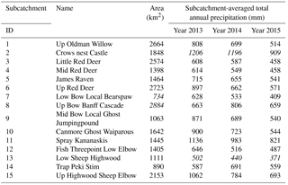
Figure 3 presents the percent bias and CRPS in five subcatchments for both GEFS and GDPS forecasts. Out of 15 subcatchments considered in this study, the maximum and minimum total annual subcatchment-averaged precipitation for the years 2013 to 2015 occurred in subcatchments 2 and 13, respectively (see Table 2); subcatchments 7 and 8 have minimum and maximum size, respectively. The four selected subcatchments covered the middle and southern portions of the study area; therefore we include subcatchment 4 to facilitate discussion on the performance of calibrated QPFs in the northern portion of the study area. The percent bias for all 15 subcatchments is provided in Fig. S1a.
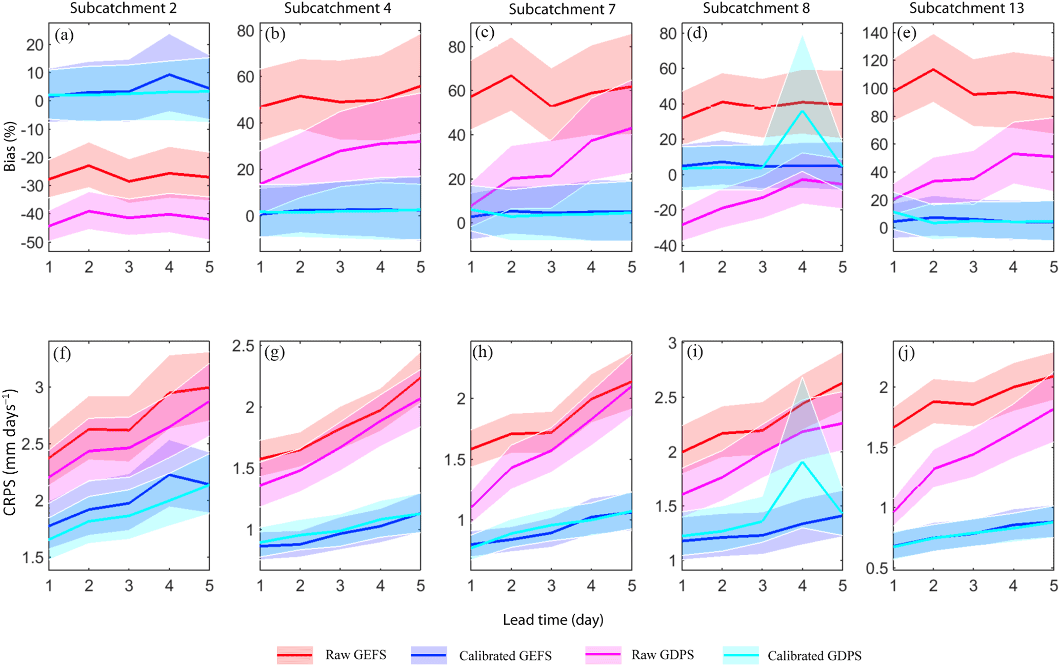
Figure 3Subcatchment-averaged bias (%) in the raw QPFs and calibrated QPFs for individual daily forecasts as a function of lead time for subcatchments 2, 4, 7, 8, and 13 (a–e, respectively); panels (f–j) show subcatchment-averaged CRPS (mm day−1) in the raw QPFs and calibrated QPFs for daily precipitation as a function of lead time. The shaded region represents 5 and 95 % confidence intervals generated using a bootstrap approach. Note the different scales on the vertical axes.
Based on visual inspection of bias plots (Fig. 3a–e), the bias in the calibrated QPF is close to zero in almost all five subcatchments (except at lead time 4 in the subcatchment 8), indicating that overall, the RPP is able to reduce the bias in the raw QPF. As shown in Fig. S1b, the inability of calibrated RPP in reproducing a peak precipitation event at lead time 4 in subcatchment 8 resulted in a large bias. The anomaly can be attributed to the fact that subcatchment 8 has the largest area and only a few observation stations lie inside the subcatchment. In the case of GEFS forecasts for the lead time of 1 day, the raw QPFs have an average bias ranging from −30 % (in subcatchment 2) to around 100 % (in subcatchment 13). In all subcatchments, the bias increases slightly from days 1 to 2, then drops on day 3 and on days 3 to 5 either increases or remains almost constant. An increase in bias in the first 2 days' lead time can be attributed to the spin-up of the NWP model. Spin-up is expected to influence only the first day or two. In the case of GDPS, the bias in the raw QPF is close to zero (except in subcatchments 2 and 8, where bias is negative) for the 1-day lead time, but the bias increases up to as high as 50 % (subcatchment 13) for a lead time of 5 days. The 5 and 95 % confidence interval around the raw QPF also increases slightly with lead time, indicating that the forecast for a lead time of 1-day will have higher confidence (hence a narrow shaded area) than for the later days, which is intuitive. It may be argued that the variations in bias in different subcatchments can be attributed to topography and physiographic characteristics. It is worth pointing out that in this study, we are not considering spatial nonstationarity because the goal is to set up a simple Bayesian model that relates the subcatchment precipitation forecasts and the observations. Accounting for the topography and elevation in the probabilistic model increases the complexity significantly and it is unlikely that the forecast performance will increase given the length of data used to infer the model parameters. Thus, we are not concerned with linking topography and corrections in the forecasts.
The subcatchment-averaged CRPSs of raw and calibrated QPFs are shown in Fig. 3f–j. It is worth mentioning that for the deterministic forecast, the CRPS reduces to the MAE; thus the plots for raw QPFs (Fig. 3f–j) show the MAE. For simplicity, we therefore refer to the MAE of raw QPFs as its CRPS. The CRPSs estimated on the calibrated QPFs are based on 1000 ensembles generated from the RPP approach. In the case of GEFS, and similar to the bias plots (Fig. 3a–e), we notice that the CRPS first increases then decreases and increases again after a lead time of 4 days in the raw QPFs. The CRPS based on the calibrated QPFs, however, consistently increases (except for subcatchment 2), indicating that as the lead time increases, deviation between forecasts and observation will be larger. In the case of GDPS, the CRPS of raw QPFs varies between 1 and 2.2 mm day−1 for a lead time of 1 day, almost linearly increasing up to 3 mm day−1 for forecast lead times of 5 days. The RPP approach reduces the CRPS significantly for each lead time in all subcatchments (except at a lead time of 4 in subcatchment 8). The reason for deviation in the CRPS at a lead time of 4 in subcatchment 8 is not trivial; however it can be attributed to RPP's inability to capture a peak precipitation event as shown in Fig. S1b. Overall the calibrated QPF has a lower CRPS than the raw QPF, which demonstrates that the RPP is able to improve the raw QPF across all lead times. The CRPSs of other subcatchments are presented in Fig. S1c.
Figure 4Relative operating characteristic (ROC) curves at lead times of 1, 3, and 5 days for calibrated QPFs for events of precipitation less than 0.2 mm and events of precipitation greater than 5 mm for subcatchment 11. Panels (a) and (b) show ROC curves of calibrated GEFS, and panels (c) and (d) show ROC curves of calibrated GDPS. In the calculation of ROC, the daily data from 2013 to 2015 are used.
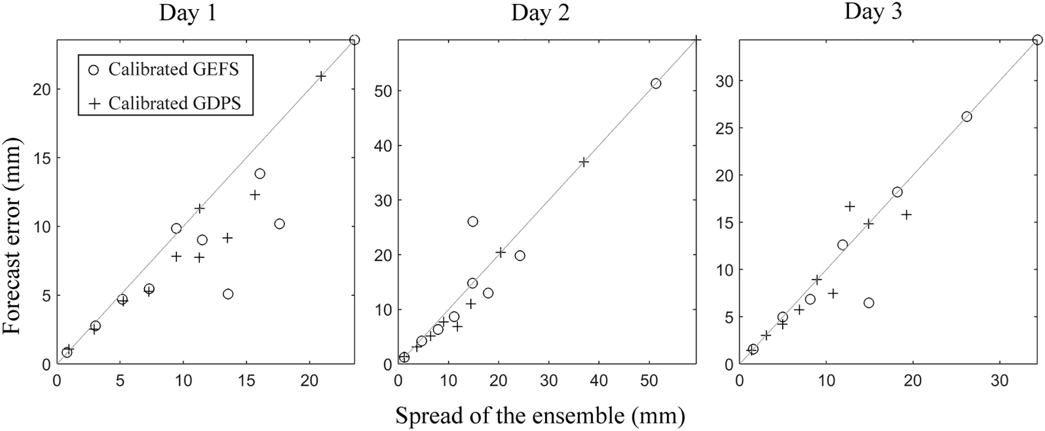
Figure 5Scatterplots of forecast error versus spread of the 100 ensembles of calibrated QPFs for lead times of 1, 3, and 5 days for subcatchment 11.
To assess the calibrated forecasts' ability to discriminate between low (< 0.2 mm) and high precipitation events (> 5 mm) for all lead times, Fig. 4 presents the ROC curves for the years 2013 to 2015. We only present results for lead times of 1, 3, and 5 days for calibrated GEFS and GDPS forecasts for subcatchment 11. The results of other subcatchments are presented in Fig. S2a–d. For GEFS (Fig. 4a and b), the ROC curves for days 1, 3, and 5 increasingly move away from the top left corner of the plot, suggesting that forecasts for shorter lead times have slightly higher discriminative ability than those for longer lead times. GDPS shows similar behavior (Fig. 4c and d), indicating that forecasts at longer lead times are less skilful than those at shorter lead times. Both GEFS and GDPS forecasts for a lead time of 1 day suggest that the forecast discrimination is stronger for higher rainfall events (> 5 mm), where ROC curves are closer to the left corner of the plot (Fig. 4c and d) than for smaller precipitation events (< 0.2 mm).
Figure 5 indicates the forecast error versus spread of the ensembles for calibrated GEFS and GDPS forecasts with lead times of 1, 3, and 5 days for subcatchment 11. For days 3 and 5, most of the points seem to fall on the diagonal (1 : 1 line), suggesting good agreement between the forecast error and the spread across all the lead times. For day 1, the deviation of the points from the diagonal (1 : 1 line) is higher, indicating a larger bias for day 1 compared to days 3 and 5. To explore this further, we calculated the frequency of observed data lying within the 10–90 % confidence boundary of calibrated QPFs. Figure 6 shows that in the case of calibrated GEFS, the calculated frequency of observed data for a lead time of 1 to 5 days varies between 0.78 and 0.88. However, for calibrated GDPS, the frequency lies between 0.87 and 0.9. Figure 6 demonstrates that as the lead time increases, the frequency of observed data lying within the [0.1–0.9] confidence boundary is higher.
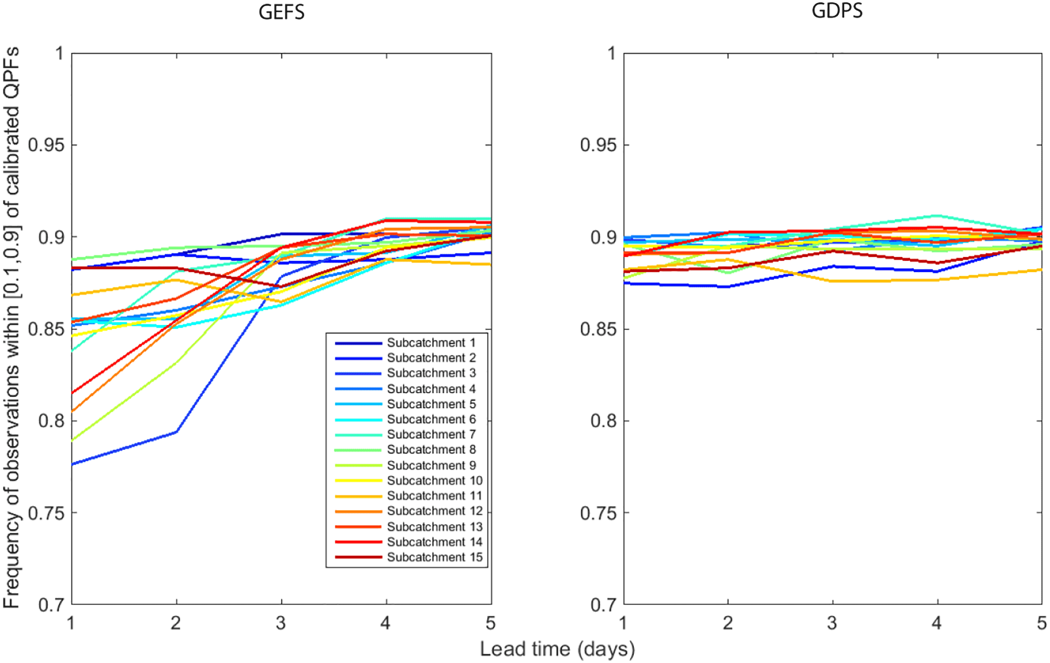
Figure 6Frequency of observations lying within the 10th and 90th percentile of calibrated GEFS and calibrated GDPS.
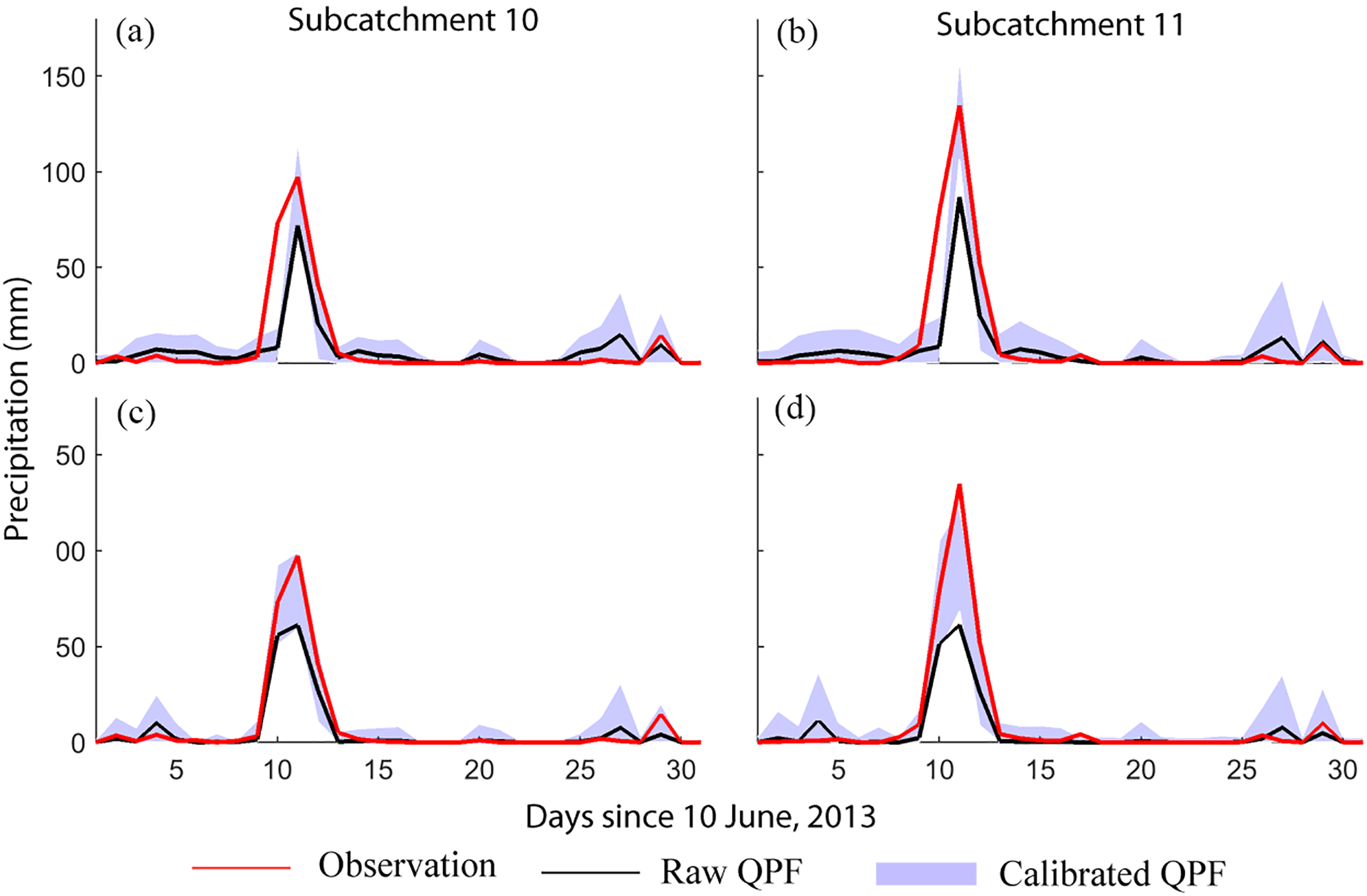
Figure 7Comparison of time series of precipitation obtained from subcatchment-averaged raw QPFs, subcatchment-averaged observations, and subcatchment-averaged calibrated QPFs in subcatchments 10 and 11. The shaded area represents the range of values obtained from 1000 post-processed ensembles. Panels (a) and (b) show results of calibrated GEFS, and panels (c) and (d) show results of calibrated GDPS.
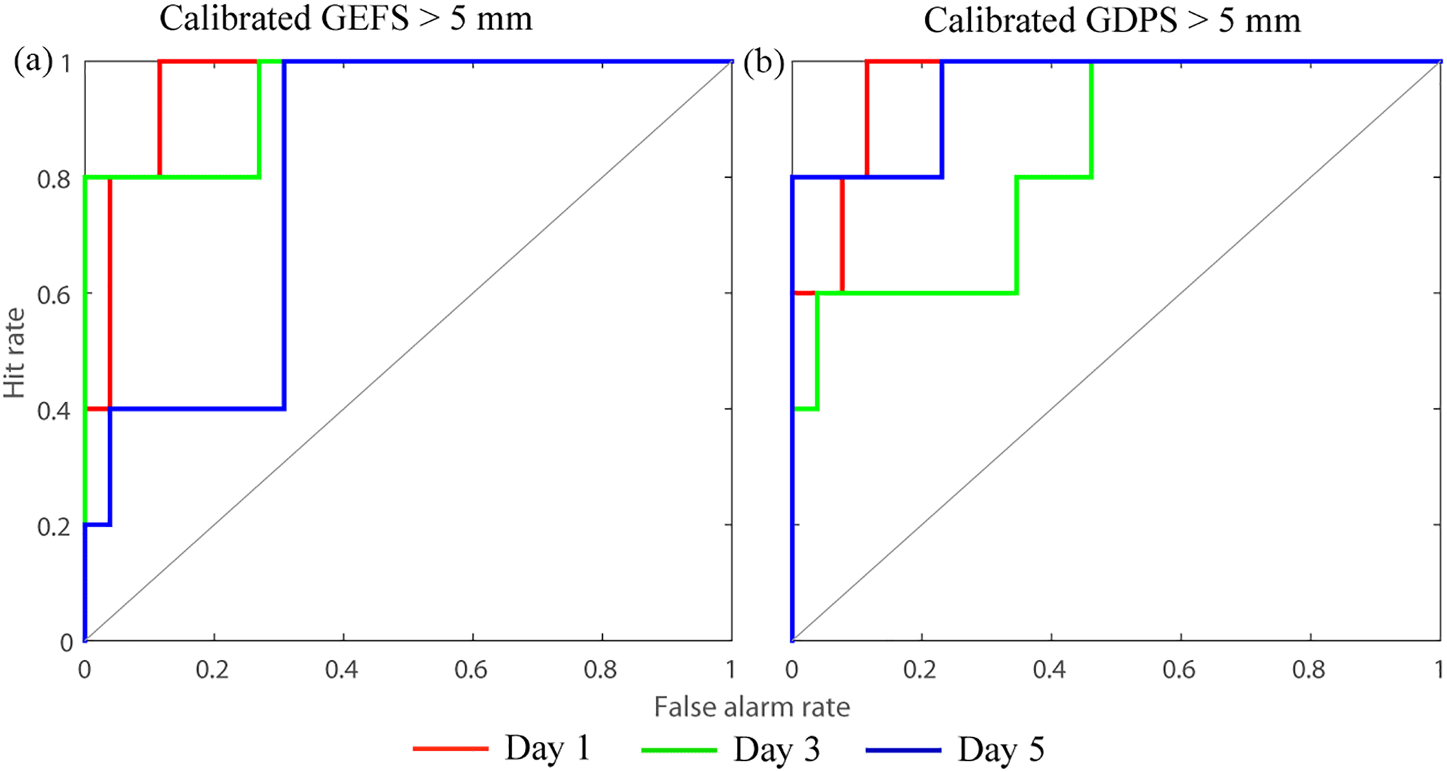
Figure 8Relative operating characteristic (ROC) curves at lead times of 1, 3, and 5 days for calibrated QPFs for precipitation events greater than 5 mm for subcatchment 11 during 10 June to 10 July 2013, with (a) and (b) showing ROC curves of calibrated GEFS and GDPS, respectively.
4.2 Performance of calibrated QPFs during an extreme event
As mentioned in Sect. 2, a severe flood event occurred from 20 to 24 June 2013 in Calgary (located near the outlet of subcatchment 7; see Fig. 1b). Therefore we examine subcatchment-averaged precipitation obtained from raw and calibrated QPFs against observed data. From the historical observed data, we notice that most peak precipitation events tend to occur over the mountains (i.e., in subcatchments 10 and 11). To consider both the peak precipitation event responsible for triggering the 2013 flood and also the series of smaller precipitation events before and after the peak event, we select a 1-month period from 10 June to 10 July 2013. Results for the 1-day lead time in subcatchments 10 and 11 (Fig. 6) relative to observed data suggest there were a series of high precipitation events on day 10, 11, and 12, with almost negligible precipitation on the remaining days relative to these peak events (with the exception of some small events on days 26 and 29). In both subcatchments 10 and 11, raw GEFS forecasts show significantly less precipitation compared to the observations from days 10 to 12 (see Fig. 7a and b). On the remaining days, raw GEFS consistently forecasts higher magnitudes of precipitation relative to the observations. The raw GDPS forecast also shows significantly lower magnitudes of precipitation relative to that observed during the peak event (days 10 to 12; Figs. 7c and d). The GDPS forecast shows overprediction of a smaller event on day 26 and underprediction on day 29. For the remaining days, the raw GDPS forecast closely matches observed precipitation. The shaded area for the calibrated QPF in the case of both GEFS and GDPS indicates the range of precipitation forecasts obtained from 1000 ensemble forecast members. In both subcatchments 10 and 11, the subcatchment-averaged calibrated QPFs (shaded area) are able to capture peak precipitation and the smaller events (except for day 10 in calibrated GEFS).
We have also evaluated the ability of the calibrated QPFs to discriminate between events and non-events for large rainfall events (> 5 mm) from 10 June to 10 July 2013. The ROC curves for lead times of 1, 3, and 5 days for both calibrated GEFS and GDPS in subcatchment 11 (Fig. 8) indicate that the calibrated GEFS (lead times of 1 and 3 days) and calibrated GDPS (lead time of 1 and 5 days) have a greater ability to discriminate between events and non-events.
Based on the results presented, the RPP shows promising performance for catchments in cold and snowy climates, such as that in western Canada. Bias-free precipitation is a vital component, among other inputs, for improved streamflow forecasts from hydrological models. For raw GEFS and GDPS, the RPP approach was able to reduce the bias in the calibrated QPFs to close to zero. The bias calculated from raw GEFS forecasts shows an almost similar bias, with slight variations, from lead times of 1 to 5 days. The GDPS forecast, however, showed an expected trend of increasing bias with increasing lead time. The advantage of applying the RPP approach was that, irrespective of the nature of the inherent bias in the raw forecasts, overall, the calibrated QPFs were bias-free.
The calibrated QPFs have significantly reduced CRPS values in all subcatchments in both GEFS and GDPS forecasts. Furthermore, the ensembles produced from the deterministic QPF were mostly able to capture the peak precipitation events within the study area (i.e., June 2013). It is noted that in the absence of ensembles, a hydrological model would take only the raw QPF and would therefore not forecast the resulting streamflow correctly during a major flood event. Ensemble precipitation forecasts would enable uncertainty bands to be produced around the forecast streamflow simulated from a hydrological model, thus increasing the chance of properly assessing the associated risks associated with sudden, high precipitation events.
ROC curves for calibrated QPFs showed that GEFS forecasts have a greater ability to discriminate between events and non-events for both low and high precipitation across all lead times. The discrimination ability of GDPS forecasts, however, reduces significantly with increasing lead time.
In conclusion, this study assessed the performance of a post-processing approach, RPP, developed in Australia, to a catchment in Alberta, Canada. The RPP approach was applied to two sets of raw forecasts, GEFS and GDPS, obtained from two different NWP models for the same periods in 2013 and 2015. In each case, 1000 post-processed forecast ensembles were created. Post-processed forecasts were demonstrated to have low bias and higher accuracy for each lead time in 15 subcatchments covering a range of topographical conditions, from mountains to western plains, inducing different precipitation mechanisms. Unlike raw forecasts, the post-processed forecast ensembles are able to capture peak precipitation events, which resulted in a major flood event in 2013 within the study area. Future work will involve applying RPP to other Canadian catchments, under different climatic conditions such as coast, plains, and the lake-dominated Boreal Shield, among others. The influence of the density of rain gauges and perhaps the use of a gridded reanalysis product for the observation dataset are left for future investigations. The authors aim to test the post-processed precipitation forecasts for streamflow forecasting in different Canadian catchments in future work.
The observed data used in this research can be obtained by submitting a data request to Alberta River Forecast Center and Environment and Climate Change Canada. The precipitation forecast, GEFS, can be directly downloaded from the website of NOAA (https://www.esrl.noaa.gov/psd/forecasts/reforecast2/). The GDPS forecast can be obtained by submitting a data request to Environment and Climate Change Canada.
The supplement related to this article is available online at: https://doi.org/10.5194/hess-22-1957-2018-supplement.
The authors declare that they have no conflict of interest.
This work was supported by the Natural Science and Engineering Research
Council of Canada and a post-doctoral fellowship under the Canadian FloodNet.
The first author would also like to acknowledge the support through the
initiation grant from the Indian Institute of Science Education and Research
Bhopal. We would like to extend our sincere honor to the late Peter
Rasmussen, who was the FloodNet Theme 3.1 project leader and actively
participated in the initial discussions. Peter Rasmussen passed away on
2 January 2017 and is greatly missed by all of us. The Alberta Forecast
Centre provided the rain gauge data and the shape files of the catchment.
Environment and Climate Change Canada provided the GDPS forecast data.
Special thanks are due to Vincent Fortin from Environment and Climate Change
Canada for helping us to properly understand the raw NWP model
output.
Edited by: Luis Samaniego
Reviewed by: Fabio Oriani and Geoff Pegram
Abaza, M., Anctil, F., Fortin, V., and Turcotte, R.: A comparison of the Canadian global and regional meteorological ensemble prediction systems for short-term hydrological forecasting, Mon. Weather Rev., 141, 3462–3476, 2013.
AEP (Alberta Environment and Parks): https://rivers.alberta.ca/, last access: February 2017.
Ahmed, S., Coulibaly, P., and Tsanis, I.: Improved Spring Peak-Flow Forecasting Using Ensemble Meteorological Predictions, J. Hydrol. Eng., 20, 04014044, https://doi.org/10.1061/(ASCE)HE.1943-5584.0001014, 2014.
AMEC: Weather Forecast Review Project for Operational Open-water River Forecasting, available at: http://aep.alberta.ca/water/programs-and-services/flood-mitigation/flood-mitigation-studies.aspx (last access: February 2017), 2014.
Atger, F.: Estimation of the reliability of ensemble-based probabilistic forecasts, Q. J. Roy. Meteor. Soc., 130, 627–646, 2004.
Bardossy, A. and Plate, E. J.: Space-time model for daily rainfall using atmospheric circulation patterns, Water Resour. Res., 28, 1247–1259, 1992.
Bennett, J. C., Robertson, D. E., Shrestha, D. L., Wang, Q., Enever, D., Hapuarachchi, P., and Tuteja, N. K.: A System for Continuous Hydrological Ensemble Forecasting (SCHEF) to lead times of 9 days, J. Hydrol., 519, 2832–2846, 2014.
Boucher, M.-A., Anctil, F., Perreault, L., and Tremblay, D.: A comparison between ensemble and deterministic hydrological forecasts in an operational context, Adv. Geosci., 29, 85–94, https://doi.org/10.5194/adgeo-29-85-2011, 2011.
Chen, J., Brissette, F. P., and Li, Z.: Postprocessing of ensemble weather forecasts using a stochastic weather generator, Mon. Weather Rev., 142, 1106–1124, 2014.
Clark, M., Gangopadhyay, S., Hay, L., Rajagopalan, B., and Wilby, R.: The Schaake shuffle: A method for reconstructing space–time variability in forecasted precipitation and temperature fields, J. Hydrometeorol., 5, 243–262, 2004.
Coulibaly, P.: Impact of meteorological predictions on real-time spring flow forecasting, Hydrol. Process., 17, 3791–3801, 2003.
Cuo, L., Pagano, T. C., and Wang, Q.: A review of quantitative precipitation forecasts and their use in short-to medium-range streamflow forecasting, J. Hydrometeorol., 12, 713–728, 2011.
Delavau, C., Chun, K., Stadnyk, T., Birks, S., and Welker, J.: North American precipitation isotope (δ18O) zones revealed in time series modeling across Canada and northern United States, Water Resour. Res., 51, 1284–1299, 2015.
Duan, Q., Sorooshian, S., and Gupta, V. K.: Optimal use of the SCE-UA global optimization method for calibrating watershed models, J. Hydrol., 158, 265–284, 1994.
Golding, B.: Quantitative precipitation forecasting in the UK, J. Hydrol., 239, 286–305, 2000.
Hamill, T. M.: Verification of TIGGE multimodel and ECMWF reforecast-calibrated probabilistic precipitation forecasts over the contiguous United States, Mon. Weather Rev., 140, 2232–2252, 2012.
Jha, S. K., Mariethoz, G., Evans, J. P., and McCabe, M. F.: Demonstration of a geostatistical approach to physically consistent downscaling of climate modeling simulations, Water Resour. Res., 49, 245–259, 2013.
Jha, S. K., Mariethoz, G., Evans, J., McCabe, M. F., and Sharma, A.: A space and time scale-dependent nonlinear geostatistical approach for downscaling daily precipitation and temperature, Water Resour. Res., 51, 6244–6261, 2015a.
Jha, S. K., Zhao, H., Woldemeskel, F. M., and Sivakumar, B.: Network theory and spatial rainfall connections: An interpretation, J. Hydrol., 527, 13–19, 2015b.
Khajehei, S.: A Multivariate Modeling Approach for Generating Ensemble Climatology Forcing for Hydrologic Applications, Dissertations and Theses, Paper 2403, https://doi.org/10.15760/etd.2400, 2015.
Khajehei, S. and Moradkhani, H.: Towards an improved ensemble precipitation forecast: A probabilistic post-processing approach, J. Hydrol., 546, 476–489, 2017.
Liu, X. and Coulibaly, P.: Downscaling ensemble weather predictions for improved week-2 hydrologic forecasting, J. Hydrometeorol., 12, 1564–1580, 2011.
Milrad, S. M., Gyakum, J. R., and Atallah, E. H.: A meteorological analysis of the 2013 Alberta flood: antecedent large-scale flow pattern and synoptic–dynamic characteristics, Mon. Weather Rev., 143, 2817–2841, 2015.
Nester, T., Komma, J., Viglione, A., and Blöschl, G.: Flood forecast errors and ensemble spread – A case study, Water Resour. Res., 48, W10502, https://doi.org/10.1029/2011WR011649, 2012.
Palmer, T. N.: The economic value of ensemble forecasts as a tool for risk assessment: From days to decades, Q. J. Roy. Meteor. Soc., 128, 747–774, 2002.
Palmer, T. N., Shutts, G. J., Hagedorn, R., Doblas-Reyes, F. J., Jung, T., and Leutbecher, M.: Representing model uncertainty in weather and climate prediction, Annu. Rev. Earth Pl. Sc., 33, 163–193, 2005.
Peel, M. C., Finlayson, B. L., and McMahon, T. A.: Updated world map of the Köppen-Geiger climate classification, Hydrol. Earth Syst. Sci., 11, 1633–1644, https://doi.org/10.5194/hess-11-1633-2007, 2007.
Pomeroy, J. W., Stewart, R. E., and Whitfield, P. H.: The 2013 flood event in the South Saskatchewan and Elk River basins: causes, assessment and damages, Can. Water Resour. J., 41, 105–117, 2016.
Qu, B., Zhang, X., Pappenberger, F., Zhang, T., and Fang, Y.: Multi-Model Grand Ensemble Hydrologic Forecasting in the Fu River Basin Using Bayesian Model Averaging, Water, 9, 74, https://doi.org/10.3390/w9020074, 2017.
Robertson, D. E., Shrestha, D. L., and Wang, Q. J.: Post-processing rainfall forecasts from numerical weather prediction models for short-term streamflow forecasting, Hydrol. Earth Syst. Sci., 17, 3587–3603, https://doi.org/10.5194/hess-17-3587-2013, 2013.
Roulin, E. and Vannitsem, S.: Postprocessing of ensemble precipitation predictions with extended logistic regression based on hindcasts, Mon. Weather Rev., 140, 874–888, 2012.
Schaake, J., Demargne, J., Hartman, R., Mullusky, M., Welles, E., Wu, L., Herr, H., Fan, X., and Seo, D. J.: Precipitation and temperature ensemble forecasts from single-value forecasts, Hydrol. Earth Syst. Sci. Discuss., 4, 655–717, https://doi.org/10.5194/hessd-4-655-2007, 2007.
Shepard, D.: A two-dimensional interpolation function for irregularly-spaced data, Proceedings of the 1968 23rd ACM national conference, 27–29 August 1968, New York, NY, USA, 517–524, https://doi.org/10.1145/800186.810616, 1968.
Shrestha, D. L., Robertson, D. E., Wang, Q. J., Pagano, T. C., and Hapuarachchi, H. A. P.: Evaluation of numerical weather prediction model precipitation forecasts for short-term streamflow forecasting purpose, Hydrol. Earth Syst. Sci., 17, 1913–1931, https://doi.org/10.5194/hess-17-1913-2013, 2013.
Shrestha, D. L., Robertson, D. E., Bennett, J. C., and Wang, Q.: Improving precipitation forecasts by generating ensembles through postprocessing, Mon. Weather Rev., 143, 3642–3663, 2015.
Tao, Y., Duan, Q., Ye, A., Gong, W., Di, Z., Xiao, M., and Hsu, K.: An evaluation of post-processed TIGGE multimodel ensemble precipitation forecast in the Huai river basin, J. Hydrol., 519, 2890–2905, 2014.
Teufel, B., Diro, G., Whan, K., Milrad, S., Jeong, D., Ganji, A., Huziy, O., Winger, K., Gyakum, J., and de Elia, R.: Investigation of the 2013 Alberta flood from weather and climate perspectives, Clim. Dynam., 48, 2881, https://doi.org/10.1007/s00382-016-3239-8, 2016.
Wang, Q. J. and Robertson, D. E.: Multisite probabilistic forecasting of seasonal flows for streams with zero value occurrences, Water Resour. Res., 47, W02546, https://doi.org/10.1029/2010WR009333, 2011.
Wang, Q. J., Robertson, D. E., and Chiew, F. H. S.: A Bayesian joint probability modeling approach for seasonal forecasting of streamflows at multiple sites, Water Resour. Res., 45, W05407, https://doi.org/10.1029/2008WR007355, 2009.
WMO: Guidelines on ensemble prediction systems and forecasting, World Meteorological Organization, Geneva, Switzerland, Geneva, Switzerland, WMO-No. 1091, 32 pp., 2012.
Wu, L., Seo, D.-J., Demargne, J., Brown, J. D., Cong, S., and Schaake, J.: Generation of ensemble precipitation forecast from single-valued quantitative precipitation forecast for hydrologic ensemble prediction, J. Hydrol., 399, 281–298, 2011.
Ye, J., Shao, Y., and Li, Z.: Flood Forecasting Based on TIGGE Precipitation Ensemble Forecast, Adv. Meteorol., 2016, 9129734, https://doi.org/10.1155/2016/9129734, 2016.
Zsótér, E., Pappenberger, F., Smith, P., Emerton, R. E., Dutra, E., Wetterhall, F., Richardson, D., Bogner, K., and Balsamo, G.: Building a Multimodel Flood Prediction System with the TIGGE Archive, J. Hydrometeorol., 17, 2923–2940, 2016.