the Creative Commons Attribution 4.0 License.
the Creative Commons Attribution 4.0 License.
 | 20 Mar 2018
Topography significantly influencing low flows in snow-dominated watersheds
Xiaohua Wei
Xin Yang
Krysta Giles-Hansen
Mingfang Zhang
Wenfei Liu
Watershed topography plays an important role in determining the spatial heterogeneity of ecological, geomorphological, and hydrological processes. Few studies have quantified the role of topography in various flow variables. In this study, 28 watersheds with snow-dominated hydrological regimes were selected with daily flow records from 1989 to 1996. These watersheds are located in the Southern Interior of British Columbia, Canada, and range in size from 2.6 to 1780 km2. For each watershed, 22 topographic indices (TIs) were derived, including those commonly used in hydrology and other environmental fields. Flow variables include annual mean flow (Qmean), Q10 %, Q25 %, Q50 %, Q75 %, Q90 %, and annual minimum flow (Qmin), where Qx % is defined as the daily flow that occurred each year at a given percentage (x). Factor analysis (FA) was first adopted to exclude some redundant or repetitive TIs. Then, multiple linear regression models were employed to quantify the relative contributions of TIs to each flow variable in each year. Our results show that topography plays a more important role in low flows (flow magnitudes ≤ Q75 %) than high flows. However, the effects of TIs on different flow magnitudes are not consistent. Our analysis also determined five significant TIs: perimeter, slope length factor, surface area, openness, and terrain characterization index. These can be used to compare watersheds when low flow assessments are conducted, specifically in snow-dominated regions with the watershed size less than several thousand square kilometres.
- Article
(3225 KB) - Full-text XML
-
Supplement
(502 KB) - BibTeX
- EndNote


Topography plays a critical role in geomorphological, biological, and hydrological processes (Moore et al., 1991; Quinn et al., 1995). Many topographic indices (TIs) have been derived to describe the spatial patterns of a landscape (Yokoyama et al., 2002), locate spatial patterns of species (Jenness, 2004), and simulate spatial soil moisture (Park et al., 2001). In hydrology, hydrological responses are forced by climatic inputs (e.g. precipitation) but are controlled by topography and other factors such as land use and land cover (Beven and Kirkby, 1979; Hewlett and Hibbert, 1967). In describing the role of topography in hydrology, numerous TIs have been developed and applied to help understand hydrological processes and to explain the variation between watersheds (Moore et al., 1991). Although the importance of topography in controlling various flow magnitudes has been widely recognized (Price, 2011), the quantitative relationship between specific TIs and various flow variables is not well understood.
TIs can be categorized into two groups, namely, primary and secondary (or compounded) indices (Moore et al., 1988). Primary indices (e.g. slope, elevation, and aspect) are normally directly calculated from a digital elevation model (DEM), while secondary indices are the combination of primary indices that are used to explain the role of topography in geomorphological, biological, and hydrological processes. For instance, the topographic wetness index (TWI) is defined as ln (α/tanβ), where α is the upslope contributing area per unit contour length and β is the slope. TWI is a required primary input for TOPMODEL and other hydrological applications (Beven, 1995; Beven and Kirkby, 1979; Quinn et al., 1995). Hydrological studies mainly focus on primary TIs and a few secondary TIs; however, these have limited explanatory power as they largely fail to explain the variation in hydrological processes. Several TIs (e.g. terrain characterization index, topographic openness) have been widely adopted in geomorphology and biology, but are seldom used in hydrological studies. A thorough examination of existing TIs is needed to identify those that best account for hydrological variations between watersheds.
Studies of watershed topography on hydrological processes often include topics such as specific discharge (Karlsen et al., 2016), spatial baseflow distribution (Shope, 2016), transit time (McGuire et al., 2005; McGuire and McDonnell, 2006), and hydrological connectivity (Jencso and McGlynn, 2011). These studies were often based on a short period of data (< 5 years), limiting our ability to draw general conclusions on how topography affects hydrological processes. Moreover, hydrological responses are compounded by the spatially diverse effects of climate, vegetation, soil, and topography (Li et al., 2017; Wei et al., 2018; Zhang et al., 2017). For example, several hydrological models have been applied to test the effects of spatial distribution of a hydrological variable (e.g. specific discharge, soil moisture, or groundwater recharge) (Erickson et al., 2005; Gómez-Plaza et al., 2001; Li et al., 2014). However, the effects of topography alone on hydrology are not usually addressed in those studies. Finally, understanding how topography influences hydrology has significant implications for sustainable management of aquatic ecosystems (Zhang et al., 2016). Therefore, the major objectives of this study were (1) to examine the role of topography in various flow magnitudes in 28 selected watersheds with snow-dominated hydrological regimes in the Southern Interior of British Columbia, Canada; and (2) to identify the most important topographic indices that can be used to compare variations in flow magnitudes between watersheds under similar climatic conditions.
2.1 Study watersheds
In this study, 28 watersheds were selected ranging in size from 2.6 to 1780 km2 (Fig. 1 and Table S1 in the Supplement). The watersheds are located between 51∘ N, 122∘ W and 49∘ N, 118∘ W in the Southern Interior of British Columbia, Canada, where hydrological regimes are snow-dominated. In this region, the Pacific Decadal Oscillation shifted from a cool to a warm phase around 1977 (Fleming et al., 2007; Wei and Zhang, 2010), resulting in more precipitation and lower temperatures, and consequently affecting hydrological regimes. In addition, an extensive mountain pine beetle infestation caused large-scale forest cover change from 2003 onwards. To avoid the uncertainties associated with these perturbations and to maximize the sample size, the period of 1989–1996 was selected, during which daily flow records of selected stations are complete. In addition, we further confirm that vegetation changes (using the leaf area index (LAI) as a proxy) did not significantly alter annual mean flow during this period (see the Supplement, Sect. S2).
Annual mean temperature (T) and precipitation (P) of the study watersheds were calculated from the ClimateBC dataset (Wang et al., 2006). ClimateBC is a stand-alone program that extracts and downscales PRISM (Daly et al., 2008) monthly climate normal data and calculates seasonal and annual climate variables for specific locations based on latitude, longitude, and elevation. Annual P, T, and potential evapotranspiration (PET) were determined at a spatial resolution of 500 m and averaged for each watershed. PET was calculated using the Hargreaves method (Liu et al., 2016; Wang et al., 2006; Zhang and Wei, 2014). The average mean annual P and PET of all 28 watersheds were 813 ± 205 and 586 ± 58 mm for 1989–1996, respectively (Figs. 1 and S1–S4).
2.2 Topographic indices
Based on availability and representation of TIs in literature, 22 topographic indices (TIs) were derived using a gridded DEM at a spatial resolution of 25 m (Table 1). The DEM, geospatial streamflow networks, and lakes and wetland coverage were obtained from GeoBC (Government of British Columbia, available at http://www2.gov.bc.ca/gov/content/data/about-data-management/geobc/geobc-products). All data were transformed to the same projected coordinate system prior to the calculations of TIs. Calculation of the TIs was made in ArcGIS 10.4.1 (ERSI®) and SAGA GIS 2.1.2. Detailed information on the calculation and interpretation of TIs can be found in the references listed in Table 1.

Figure 1Locations and elevations of the 28 study watersheds, and their hydrometric stations (red star symbols).
Table 1Topographic indices and descriptions.
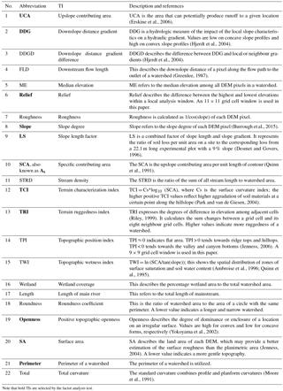
Note that bold TIs are selected by the factor analysis test.
3.1 Definitions of the selected flow variables
Annual mean flow (Qmean) and other flow variables generated by the annual flow duration curve were used in this study. The selected flow variables include Q10 %, Q25 %, Q50 %, Q75 %, Q90 %, and annual minimum flow (Qmin) (mm day−1). They are defined as the daily flow that occurred each year at the given percentage. For example, Q90 % is the flow magnitude at 90 % of the time in a year (Cheng et al., 2012). To account for the confounding effects of climate, each annual flow variable was standardized with annual (P) and expressed as QX∕P.
3.2 Factor analysis
Because some initially selected TIs may be highly related, the first step was to introduce factor analysis (FA) to reduce the number of TIs while still retaining important topographic information. FA can be interpreted in a similar manner as principal component analysis. The major difference between the two approaches is that FA not only considers the total variance but also makes the distinction between common and unique variance (Lyon et al., 2012). As TIs were calculated in a region with similar topography, the average TIs at the watershed level are not varied dramatically between watersheds (McGuire and McDonnell, 2006; Price, 2011). Therefore, to ensure better differentiation, the standard deviations of TIs of a watershed were used for the FA test. It should be noted that the flow variables were not included in the FA test.
Three criteria were used in the FA procedure to exclude redundant TIs: the Kaiser–Meyer–Olkin (KMO) test, Bartlett's test, and anti-image correlation. KMO is a measure of sampling adequacy which tests whether partial correlations among variables are small enough to ensure the validity of the FA test. Bartlett's test of sphericity assesses the level of correlation between the variables in the FA to determine if the combination of variables is suitable for such analysis (Lyon et al., 2012). The diagonals of the anti-image correlation matrix are a measure of sampling adequacy of specific TIs, which ensures that TIs are adequate for the FA. If a TI makes the FA indefinite, namely KMO < 0.7, Bartlett's test P > 0.05, and the diagonals of anti-image correlation < 0.7, then this TI is excluded from further consideration. With this iterative approach, the group of TIs with the largest KMO, Bartlett's test P < 0.05, and the diagonals of anti-image correlation > 0.7 are determined as the final group of TIs. In this study, FA tests were conducted in the IBM® SPSS® Statistics Version 22.
3.3 Relative contributions of each TI to flow variables
The nonparametric Kendall's tau correlation examined the statistical correlations between flow variables and the FA-selected TIs in the 28 study watersheds. If a significant correlation is detected, it indicates high topographic control on that flow variable. Multiple linear regression (MLR) models were then built for each year between 1989 and 1996 for each flow variable (see Sect. 5 in the Supplement for details). The purposes of the MLR models were (1) to further exclude those TIs that were insignificantly related to flow variables, and (2) to quantify the relative contributions of the selected TIs to each flow variable in each year. In the MLR models, each flow variable was treated as a dependent variable, while all FA-selected TIs were regarded as independent variables. To exclude insignificant TIs to flow variables, all the 11 selected TIs by the FA were initially included in the MLR model. The ANOVA (analysis of variance) test was then adopted to identify the statistical significance between TIs and each flow variable in each year. If one TI was insignificant (P > 0.05), then it was removed from the model. The ANOVA test was then re-run for the rest of the TIs to ensure that all significant TIs were selected. By this trial and error process, the final models with only significant TIs to flow variables were determined. The detailed procedure can also be found in Li et al. (2014). Then, the R package “relaimpo” was used to quantify the relative contributions of the selected TIs to each flow variable (Gromping, 2006). In particular, the relative contributions of each dependent variable to R2 were calculated for each model. In this way, the contributions of the significant TIs to flow variables were derived for each MLR model.
To quantify the role of each TI in regulating each flow variable, we defined a contribution index (CI), which can be expressed as CI = O×C, where O is the number of the selected TIs appearing in the final MLR models (the maximum number is eight because each flow variable is studied for 8 years), and C is the average relative contribution of each TI to the specific flow variable . Therefore, a higher CI indicates a higher influence of that TI on a flow variable. The lumped CI of each TI to each flow variable is treated as the total contribution of the TI to all flow variables. Finally, the TIs with the CI values that are higher than the average of the lumped CI of all TIs were determined as the final set of TIs. As such, TIs with higher contributions were selected for the flow variables.
4.1 Factor analysis
A subset of 11 TIs was selected from the initial 22 calculated TIs using the FA procedure. The KMO test (0.853), Bartlett's test (P < 0.001), and the diagonals of anti-image correlation (> 0.7) on the 11 TIs further confirm that our selected TIs are adequate to represent topographical characteristics of a watershed in our study region. In the FA analysis, the first and second factors explained 80.9 and 11.7 % of total variance of TIs in the selected watersheds, respectively (Fig. 2). TIs included in the first factor are DDG, LS, openness, relief, slope, SA, TCI, and TRI, while those in the second factor include SCA, perimeter, and UCA. Based on the definition of each TI, we further conclude that the first factor represents watershed roughness or complexity, while the second factor describes the watershed size. Therefore, the selected 11 TIs were subsequently classified into two groups representing complexity (Group A) and area (Group B) (Fig. 2).
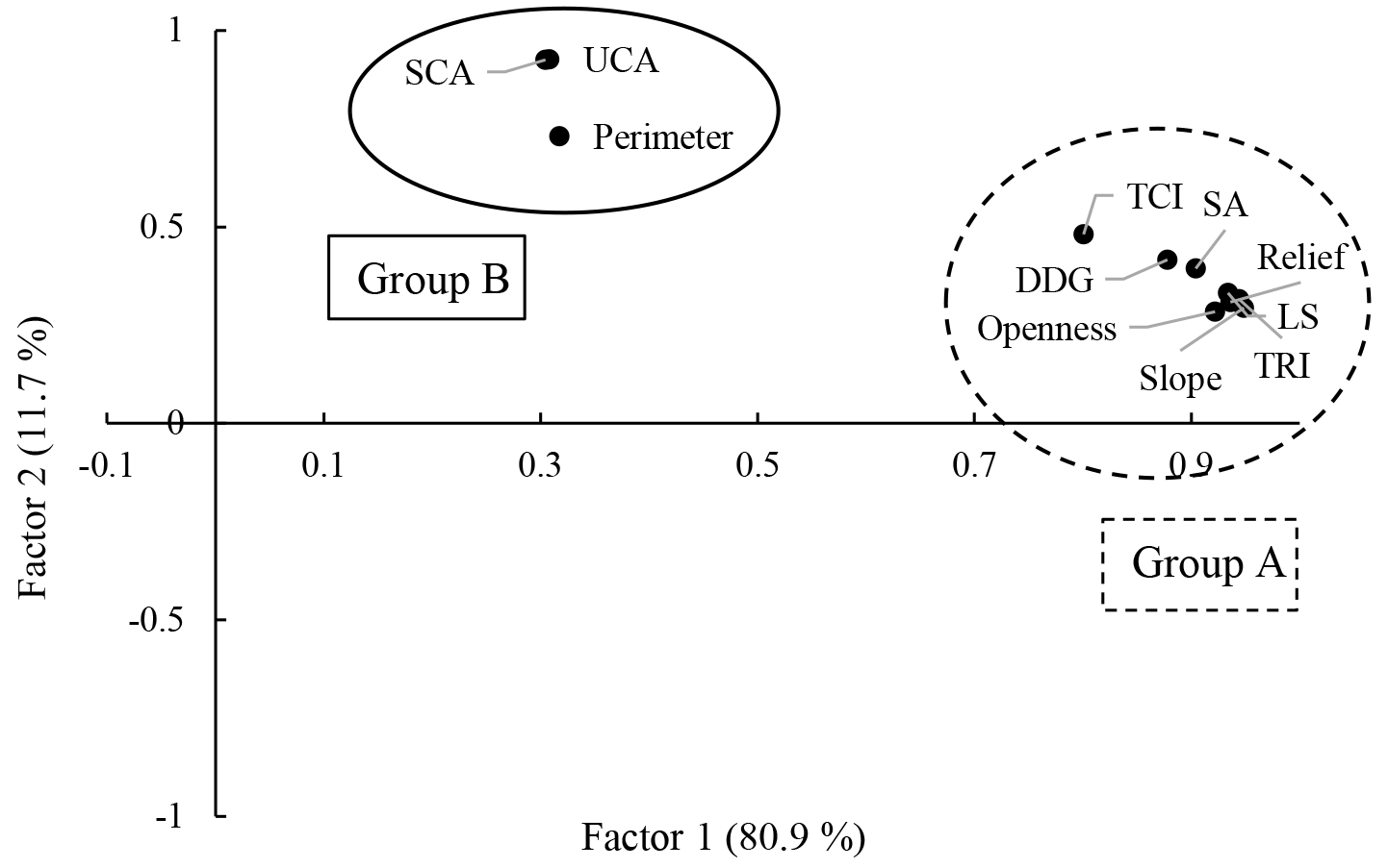
Figure 2Factor analysis of topographic indices (TIs) among 28 watersheds. The first and second factors explained 80.9 and 11.7 % of the total variance, respectively.
4.2 Relative contributions of TIs to flow variables
The nonparametric Kendall's tau test revealed significant correlations between the TIs and each flow variable from 1989 to 1996 (Tables S2 to S8). The number of significant TIs in each year increased from 1 to 11 with decreasing flow magnitudes. A larger number of the TIs were correlated to low flow variables (Q75 %, Q90 %, and Qmin), indicating that topography plays a more pronounced role in regulating lower flows. Here, flows lower than or equal to Q75 % are defined as the low flows. Thus, MLR models were only carried out for Q75 %, Q90 %, and Qmin.
The regression models between flow variables and the selected TIs were all significant (P < 0.01) with R2 values ∼ 0.5, indicating that selected TIs can be used to explain the variations of flow variables (Table S9). The details of MLR models are listed in the Supplement. The TIs that were included in each model are shown in Fig. 3 and Tables S10–S13. The relative contributions of each TI to Q75 %, Q90 %, and Qmin showed large variations between years (Fig. 3a to c, and Tables S10–S12). Figure 3 revealed that each TI influences flow variables differently (e.g. SA played a prominent role in Q90 % but did not significantly contribute to the variation of Qmin, while openness had the opposite role). This means that each TI cannot be used to explain variation in the same way for each flow variable. Based on the lumped CI values, the relative contribution of the perimeter TI was the highest in Group B as well as among all TIs (Fig. 3d). In Group A, the TIs above the average of the lumped CI were LS, SA, openness, and TCI receiving high contributions to low flows. Therefore, we conclude that the five above-mentioned TIs are significant topographic indices influencing low flow variables, which can be used to assess and compare low flows in any watershed studies where there are similarities in watershed size and climate.
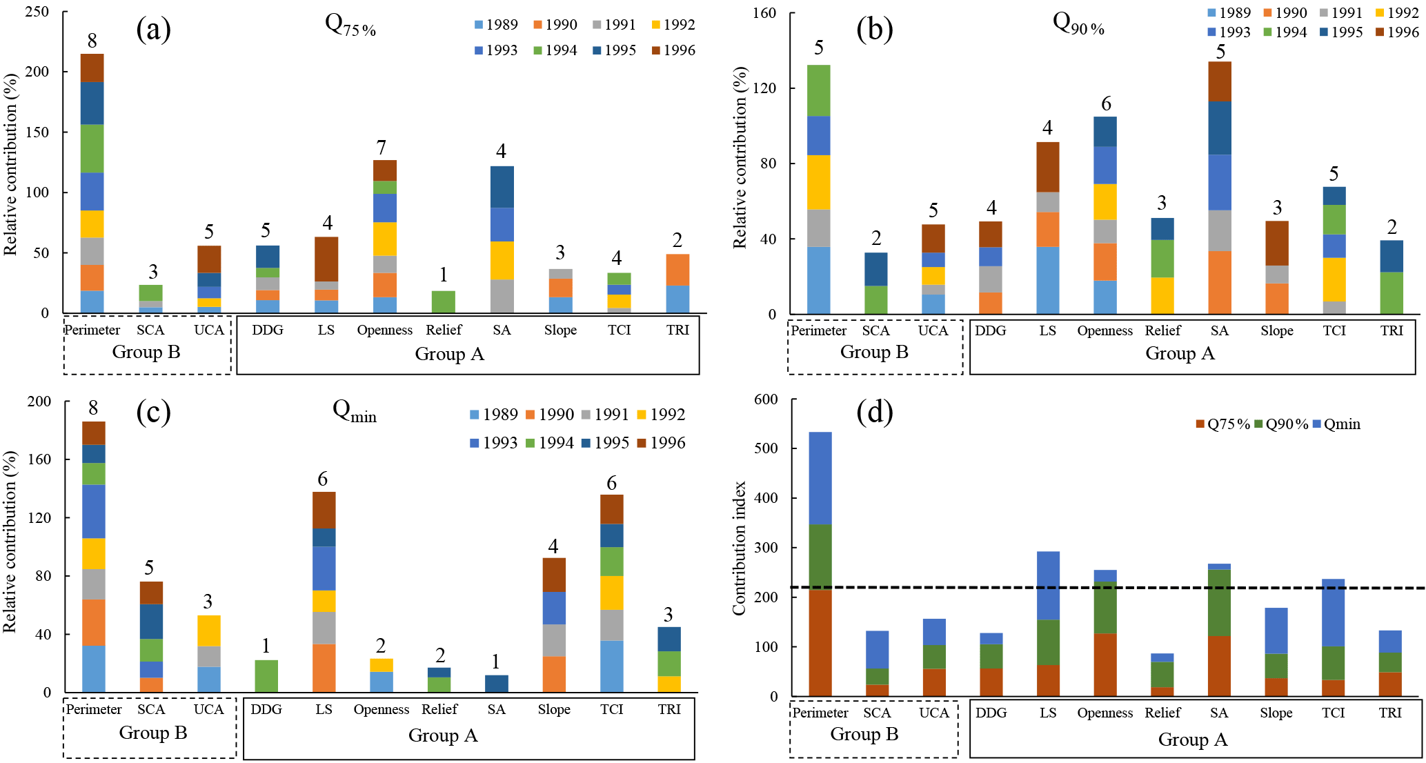
Figure 3Relative contributions of each topographic index (TI) to Q75 % (a), Q90 % (b), and Qmin (c) from 1989 to 1996. Note that the numbers above the bars indicate the number of years when the given TIs were included in the regression models. (d) Contribution index (CI) of the 11 topographic indices (TIs) selected by factor analysis (FA) to Q75 %, Q90 %, and Qmin respectively. The dashed line is the average of the lumped CI.
In this study, our results show that a limited number of TIs are significantly related to the Qmean, Q10 %, and Q25 %, suggesting that topography plays a limited role in the variations of annual mean flow and high flows. This study area is characterized by snow-dominated hydrological regimes, with high flows (e.g. Q25 % or greater) coming predominantly from the snowmelt process in early March to late May (e.g. Fig. S6). Snowmelt processes are significantly related to elevation and climate in our study region (Winkler et al., 2005). As the study watersheds in the Southern Interior of British Columbia, Canada, have similar elevation ranges and climate variability, it is not surprising that only a limited number of TIs were significantly related to high or mean flows. In contrast, more TIs were significantly associated with low flows, suggesting that topography plays a more important role in low flows than high flows in the study region. Low flows often occur in the later summer (late August) and winter (October to February) (e.g. Fig. S6) and are mainly driven by groundwater discharges and small amounts of precipitation. A watershed with more complexities of topography would likely have a higher water retention ability due to longer flow paths and residence time and consequently promote more groundwater recharge and higher low flows (Price, 2011). Our Kendall's tau correlation tests uncover a positive relationship between the selected TIs and low flow variables (Tables S6–S8), indicating that the rougher or more complex that a watershed is, the higher the low flow yields are. Therefore, we conclude that topography plays a more important role in low flows than in high flows in the study region.
Five TIs including perimeter, LS, SA, openness, and TCI were identified as the major contributors to flow variables in this study. As far as we know, no studies have quantified topographic controls on various flow magnitudes. Nevertheless, the relationship between topography and the mean transit time (McGuire and McDonnell, 2006), temporal specific discharge (Karlsen et al., 2016), and hydrological connectivity (Jencso and McGlynn, 2011) have been investigated. There is no doubt that topography is one of the major contributors to hydrological variations (Price, 2011; Smakhtin, 2001). Although these studies pinpointed specific TIs and their interactions with hydrological responses, only a limited number of TIs were quantitatively assessed. In contrast, a total number of 22 TIs were calculated for 28 watersheds in this study. The much higher number of TIs that were initially included, along with the filtering methods applied, allowed us to select more suitable and significant TIs. Through this study design, we expect that the five selected TIs can effectively be used to support assessment or comparisons of low flows between watersheds in the study region. It should also be noted that we only selected the first five TIs that had substantially higher contributions than the other calculated TIs. The rest of the hydrological-related TIs showed only a minor ability to explain flow variations.
Among the five selected TIs, the perimeter, a primary TI, is commonly used in scientific studies to describe the characteristics of watershed topography. Our study further proves that it has a large influence on low flow variables. However, four secondary TIs (LS, SA, openness, and TCI) are mainly used in geomorphology to characterize ruggedness or roughness of landscapes and to identify topographic functioning of ecosystems. For examples, TCI has been used to map soil organic matter concentration (Zeng et al., 2016). Park et al. (2001) revealed that TCI is a better TI to predict soil depth than TWI, plan curvature, and profile curvature (see definitions in Table 1). LS is one of the key inputs to the Universal Soil Loss Equation being used to quantify soil erosion hazards (Desmet and Govers, 1996). SA was used to estimate animal species and habitat (Jenness, 2004) and map the spatial patterns of a floodplain (Scown et al., 2015). Openness was initially adopted to identify the boundary of different geological units and can be used to identify surface convexities and concavities, which is better than the commonly used profile and plan curvature (Yokoyama et al., 2002). In this study, the five selected TIs were initially filtered by the FA test, indicating that each selected TI has uniqueness in describing watershed topographic characteristics and outperformed the other tested TIs in describing variation in flow variables in our study region. Therefore, we expect that the five selected TIs can be applied to support hydrological analysis and modelling.
To our surprise, some commonly used TIs in hydrology, such as slope, median elevation, upslope contribution area, and wetland areas are not included in the FA list as the topographic information contained in those primary TIs also exists in some secondary TIs. Secondary TIs have the advantage of describing the hydrology-related landscapes in fuller detail. For example, slope is directly included in calculations of the TWI (secondary) and DDG (secondary). UCA (primary TI) is included in TWI and TCI (secondary). It is also worth mentioning that some secondary TIs played critical roles in determining the spatial heterogeneity of ecological and geomorphological processes, but their roles in hydrological processes in our study region were not demonstrated. These TIs were, therefore, not selected in this study. For example, the TWI has long been used as a key input variable for TOPMODEL and is an indicator of soil moisture (Beven, 1995). Our study identified that TWI and wetland area were not significantly related to flow variables, indicating that these factors played a limited role in the selected flow variables in our region. This may be because the watersheds in this area need to overcome a soil moisture storage threshold prior to releasing water (Karlsen et al., 2016). In summary, our selected five TIs significantly represent low flow characteristics of the watersheds in the Southern Interior of British Columbia, Canada, which is characterized by a snow-dominated hydrological regime.
In our study, FA was first introduced to exclude reductant TIs. The MLR models were further employed to exclude the insignificant TIs to various flow magnitudes. There is a concern whether the TIs excluded by FA were significantly related to flow magnitudes but not included in the MLR models. To address this concern, we re-ran a subset of analyses by conducting the MLR models for Qmin in 1989, 1990, and 1991 as examples (Sect. 6 in the Supplement). The results showed that the MLR models would include several redundant TIs (e.g. wetland coverage, roundness, stream length) if the FA test were not conducted (Table S14). The Kendall's tau correlation tests uncovered that they were not significantly correlated with low flows (Table S8). This further demonstrates that some redundant and nonsignificant TIs would be introduced if the FA test were not initially conducted. In addition, our research framework was developed based on a large number of watersheds with long-term hydrological data, all in a similar climatic region that is snow-dominated. As far as we know, there are no such studies conducted in either snow- or rain-dominated regions. Our research methodology or framework can be applied in rain-dominated regions to assess how topography controls flow in any regions where there are sufficient long-term monitoring data.
There are several uncertainties in our study. Firstly, hydrological responses are the resultant effects of climate, soil, vegetation, topography, and geology (Price, 2011; Smakhtin, 2001). In this study, the LAI, which represented the variations of vegetation cover in different watersheds, was included in our analysis in order to minimize the effects of different levels of vegetation coverage in the study watersheds. However, it was excluded by the FA test, confirming that the differences in vegetation cover and their effects were minor; therefore our selected watersheds are comparable in terms of forest coverage. In addition, the climate could be a confounding factor affecting our comparisons. In this study, annual flow variables were standardized by the annual precipitation to minimize the effects of climate on flow variables. In this way, the effects of climate variability were considered to some extent, but not in full detail. For examples, in extreme dry or wet years (e.g. 1994 and 1996 are the driest and wettest years in our study period, respectively) (Figs. S2–S5), hardly any of the TIs were significantly correlated to Q90 % (Table S7), but almost all were correlated to Qmin (Table S8). This is because that the flows at Q90 % in 1994 and 1996 in the selected watersheds occurred in the winter (October–February) (e.g. Fig. S6), while the flows at Qmin in the majority of watersheds were in the late summer (August and September). The Kendall's tau correlation tests also confirm that topography played a minor role in Q90 % (Table S7), but a significant role in Qmin (Table S8). Thus, hydrological responses are mainly controlled by the combined effects of climate and topography. Secondly, LS and TCI are commonly used indicators of soil erodibility and were included in this study to capture the influence of soil conditions. For example, Park et al. (2001) showed that the areas with high values of TCI have high rates of soil erosion. Therefore, the variation of soil properties was considered to some degree by the inclusion of these TIs, but not in full detail. In fact, it is impossible to derive accurate soil properties over a large area. Thirdly, potential impacts of the DEM resolution on the calculation of TIs were not considered. However, Panagos et al. (2015) indicated that the resolution of 25 m is adequate for the calculation of slope factor at the European scale. Similarly, DEM resolutions were not found to significantly affect the calculation of DDG (Hjerdt et al., 2004). Thus, considering the same DEM data with the resolution of 25 m, we assume that the error caused by the DEM resolution would also be minor.
This study concludes that topography plays a significant role in low flows, while its role in high flows is limited. A total number of five topographic indices, including perimeter, LS (slope length factor), SA (surface area), openness, and TCI (topographic characteristic index), were identified with significant contributions to low flow variables. It is recommended that these five above-mentioned TIs can be used to assess the magnitude of low flows in a study region which is characterized by a snow-dominated hydrological regime with watershed sizes up to several thousand square kilometres. Our research methodology can be applied to other regions for investigating how topography controls flow magnitudes.
Topographic indices of study watersheds are freely available upon request by sending an email to the corresponding author.
The supplement related to this article is available online at: https://doi.org/10.5194/hess-22-1947-2018-supplement.
The authors declare that they have no conflict of interest.
We thank Environment Canada and GeoBC for their data on streamflow and DEM.
The authors would also like to thank the editor (Thom Bogaard) and two
reviewers (Petra Hulsman and Niclas Hjerdt) for their constructive comments on the
earlier version of the paper. The research funding for supporting this
project was provided by the Natural Sciences and Engineering Research Council
of Canada (RGPIN-2015-06032), the National Natural Science Foundation of
China (numbers 41771415 and 31770759), and the Priority Academic Program
Development of Jiangsu Higher Education Institutions (number:
164320H116).
Edited by: Thom
Bogaard
Reviewed by: Niclas Hjerdt and Petra Hulsman
Ambroise, B., Beven, K., and Freer, J.: Toward a generalization of the TOPMODEL concepts: Topographic indices of hydrological similarity, Water Resour. Res., 32, 2135–2145, 1996.
Beven, K.: Linking Parameters across Scales – Subgrid Parameterizations and Scale-Dependent Hydrological Models, Hydrol Process, 9, 507–525, https://doi.org/10.1002/hyp.3360090504, 1995.
Beven, K. and Kirkby, M. J.: A physically based, variable contributing area model of basin hydrology/Un modèle à base physique de zone d'appel variable de l'hydrologie du bassin versant, Hydrolog. Sci. J., 24, 43–69, 1979.
Burrough, P. A., McDonnell, R., McDonnell, R. A., and Lloyd, C. D.: Principles of geographical information systems, Oxford University Press, 2015.
Cheng, L., Yaeger, M., Viglione, A., Coopersmith, E., Ye, S., and Sivapalan, M.: Exploring the physical controls of regional patterns of flow duration curves – Part 1: Insights from statistical analyses, Hydrol. Earth Syst. Sci., 16, 4435–4446, https://doi.org/10.5194/hess-16-4435-2012, 2012.
Daly, C., Halbleib, M., Smith, J. I., Gibson, W. P., Doggett, M. K., Taylor, G. H., Curtis, J., and Pasteris, P. P.: Physiographically sensitive mapping of climatological temperature and precipitation across the conterminous United States, Int. J. Climatol., 28, 2031–2064, 10.1002/joc.1688, 2008.
Desmet, P. J. J. and Govers, G.: A GIS procedure for automatically calculating the USLE LS factor on topographically complex landscape units, J. Soil Water Conserv., 51, 427–433, 1996.
Erickson, T. A., Williams, M. W., and Winstral, A.: Persistence of topographic controls on the spatial distribution of snow in rugged mountain terrain, Colorado, United States, Water Resour. Res., 41, W04014, https://doi.org/10.1029/2003wr002973, 2005.
Erskine, R. H., Green, T. R., Ramirez, J. A., and MacDonald, L. H.: Comparison of grid-based algorithms for computing upslope contributing area, Water Resour. Res., 42, W09416, https://doi.org/10.1029/2005WR004648, 2006.
Fleming, S. W., Whitfield, P. H., Moore, R. D., and Quilty, E. J.: Regime-dependent streamflow sensitivities to Pacific climate modes cross the Georgia-Puget transboundary ecoregion, Hydrol. Process., 21, 3264–3287, https://doi.org/10.1002/hyp.6544, 2007.
Gómez-Plaza, A., Martınez-Mena, M., Albaladejo, J., and Castillo, V.: Factors regulating spatial distribution of soil water content in small semiarid catchments, J. Hydrol., 253, 211–226, 2001.
Greenlee, D. D.: Raster and vector processing for scanned linework, Photogramm. Eng. Rem. S., 53, 1383–1387, 1987.
Gromping, U.: Relative importance for linear regression in R: The package relaimpo, J. Stat. Softw., 17, 27, https://doi.org/10.18637/jss.v017.i01, 2006.
Hewlett, J. D. and Hibbert, A. R.: Factors affecting the response of small watersheds to precipitation in humid areas, Forest Hydrology, 1, 275–290, 1967.
Hjerdt, K. N., McDonnell, J. J., Seibert, J., and Rodhe, A.: A new topographic index to quantify downslope controls on local drainage, Water Resour. Res., 40, W0560, https://doi.org/10.1029/2004wr003130, 2004.
Jencso, K. G. and McGlynn, B. L.: Hierarchical controls on runoff generation: Topographically driven hydrologic connectivity, geology, and vegetation, Water Resour. Res., 47, W11527 https://doi.org/10.1029/2011wr010666, 2011.
Jenness, J.: Topographic Position Index (tpi_jen. avx) extension for ArcView 3. x, v. 1.3 a. Jenness Enterprises, available at: http://www.jennessent.com/arcview/tpi.htm (last access: 16 March 2018), 2006.
Jenness, J. S.: Calculating landscape surface area from digital elevation models, Wildlife Soc. B., 32, 829–839, https://doi.org/10.2193/0091-7648(2004)032[0829:Clsafd]2.0.Co;2, 2004.
Karlsen, R. H., Grabs, T., Bishop, K., Buffam, I., Laudon, H., and Seibert, J.: Landscape controls on spatiotemporal discharge variability in a boreal catchment, Water Resour. Res., 52, 6541–6556, https://doi.org/10.1002/2016WR019186, 2016.
Li, Q., Qi, J. Y., Xing, Z. S., Li, S., Jiang, Y. F., Danielescu, S., Zhu, H. Y., Wei, X. H., and Meng, F. R.: An approach for assessing impact of land use and biophysical conditions across landscape on recharge rate and nitrogen loading of groundwater, Agr. Ecosyst. Environ., 196, 114–124, https://doi.org/10.1016/j.agee.2014.06.028, 2014.
Li, Q., Wei, X., Zhang, M., Liu, W., Fan, H., Zhou, G., Giles-Hansen, K., Liu, S., and Wang, Y.: Forest cover change and water yield in large forested watersheds: A global synthetic assessment, Ecohydrology, 10, e1838, https://doi.org/10.1002/eco.1838, 2017.
Liu, W., Wei, X., Li, Q., Fan, H., Duan, H., Wu, J., Giles-Hansen, K., and Zhang, H.: Hydrological recovery in two large forested watersheds of southeastern China: the importance of watershed properties in determining hydrological responses to reforestation, Hydrol. Earth Syst. Sci., 20, 4747–4756, https://doi.org/10.5194/hess-20-4747-2016, 2016.
Lyon, S. W., Nathanson, M., Spans, A., Grabs, T., Laudon, H., Temnerud, J., Bishop, K. H., and Seibert, J.: Specific discharge variability in a boreal landscape, Water Resour. Res., 48, W08506, https://doi.org/10.1029/2011wr011073, 2012.
McGuire, K. J. and McDonnell, J. J.: A review and evaluation of catchment transit time modeling, J. Hydrol., 330, 543–563, 10.1016/j.jhydrol.2006.04.020, 2006.
McGuire, K. J., McDonnell, J. J., Weiler, M., Kendall, C., McGlynn, B. L., Welker, J. M., and Seibert, J.: The role of topography on catchment-scale water residence time, Water Resour. Res., 41, W05002, https://doi.org/10.1029/2004wr003657, 2005.
Moore, I., Burch, G., and Mackenzie, D.: Topographic effects on the distribution of surface soil water and the location of ephemeral gullies, Trans. ASAE, 31, 1098–1107, 1988.
Moore, I. D., Grayson, R. B., and Ladson, A. R.: Digital Terrain Modeling – a Review of Hydrological, Geomorphological, and Biological Applications, Hydrol. Process., 5, 3–30, https://doi.org/10.1002/hyp.3360050103, 1991.
Panagos, P., Borrelli, P., and Meusburger, K.: A new European slope length and steepness factor (LS-Factor) for modeling soil erosion by water, Geosciences, 5, 117–126, 2015.
Park, S. J. and van de Giesen, N.: Soil-landscape delineation to define spatial sampling domains for hillslope hydrology, J. Hydrol., 295, 28–46, https://doi.org/10.1016/j.jhydrol.2004.02.022, 2004.
Park, S. J., McSweeney, K., and Lowery, B.: Identification of the spatial distribution of soils using a process-based terrain characterization, Geoderma, 103, 249–272, https://doi.org/10.1016/S0016-7061(01)00042-8, 2001.
Price, K.: Effects of watershed topography, soils, land use, and climate on baseflow hydrology in humid regions: A review, Prog. Phys. Geog., 35, 465–492, 2011.
Quinn, P., Beven, K., Chevallier, P., and Planchon, O.: The Prediction of Hillslope Flow Paths for Distributed Hydrological Modeling Using Digital Terrain Models, Hydrol. Process., 5, 59–79, https://doi.org/10.1002/hyp.3360050106, 1991.
Quinn, P. F., Beven, K. J., and Lamb, R.: The Ln(a/Tan-Beta) Index – How to Calculate It and How to Use It within the Topmodel Framework, Hydrol. Process., 9, 161–182, https://doi.org/10.1002/hyp.3360090204, 1995.
Riley, S. J.: Index That Quantifies Topographic Heterogeneity, Intermountain Journal of Sciences, 5, 23–27, 1999.
Scown, M. W., Thoms, M. C., and De Jager, N. R.: Measuring floodplain spatial patterns using continuous surface metrics at multiple scales, Geomorphology, 245, 87–101, 10.1016/j.geomorph.2015.05.026, 2015.
Shope, C. L.: Disentangling event-scale hydrologic flow partitioning in mountains of the Korean Peninsula under extreme precipitation, J. Hydrol., 538, 399–415, https://doi.org/10.1016/j.jhydrol.2016.04.050, 2016.
Smakhtin, V. U.: Low flow hydrology: a review, J. Hydrol., 240, 147–186, https://doi.org/10.1016/S0022-1694(00)00340-1, 2001.
Wang, T., Hamann, A., Spittlehouse, D. L., and Aitken, S. N.: Development of scale-free climate data for western Canada for use in resource management, Int. J. Climatol., 26, 383–397, https://doi.org/10.1002/Joc.1247, 2006.
Wei, X., Li, Q., Zhang, M., Giles-Hansen, K., Liu, W., Fan, H., Wang, Y., Zhou, G., Piao, S., and Liu, S.: Vegetation cover – another dominant factor in determining global water resources in forested regions, Glob. Change Biol., 24, 786–795, https://doi.org/10.1111/gcb.13983, 2018.
Wei, X. H. and Zhang, M. F.: Quantifying streamflow change caused by forest disturbance at a large spatial scale: A single watershed study, Water Resour. Res., 46, W12525, https://doi.org/10.1029/2010wr009250, 2010.
Winkler, R. D., Spittlehouse, D. L., and Golding, D. L.: Measured differences in snow accumulation and melt among clearcut, juvenile, and mature forests in southern British Columbia, Hydrol. Process., 19, 51–62, https://doi.org/10.1002/hyp.5757, 2005.
Yokoyama, R., Shirasawa, M., and Pike, R. J.: Visualizing topography by openness: a new application of image processing to digital elevation models, Photogramm. Eng. Rem. S., 68, 257–266, 2002.
Zeng, C. Y., Yang, L., Zhu, A. X., Rossiter, D. G., Liu, J., Liu, J. Z., Qin, C. Z., and Wang, D. S.: Mapping soil organic matter concentration at different scales using a mixed geographically weighted regression method, Geoderma, 281, 69–82, https://doi.org/10.1016/j.geoderma.2016.06.033, 2016.
Zhang, M. and Wei, X.: Contrasted hydrological responses to forest harvesting in two large neighbouring watersheds in snow hydrology dominant environment: implications for forest management and future forest hydrology studies, Hydrol. Process., 28, 6183–6195, https://doi.org/10.1002/hyp.10107, 2014.
Zhang, M., Wei, X., and Li, Q.: A quantitative assessment on the response of flow regimes to cumulative forest disturbances in large snow-dominated watersheds in the interior of British Columbia, Canada, Ecohydrology, 9, 843–859, https://doi.org/10.1002/eco.1687, 2016.
Zhang, M. F., Liu, N., Harper, R., Li, Q., Liu, K., Wei, X. H., Ning, D. Y., Hou, Y. P., and Liu, S. R.: A global review on hydrological responses to forest change across multiple spatial scales: Importance of scale, climate, forest type and hydrological regime, J. Hydrol., 546, 44–59, https://doi.org/10.1016/j.jhydrol.2016.12.040, 2017.