Wetlands inform how climate extremes influence surface water expansion and contraction

Effective monitoring and prediction of flood and drought events requires an improved understanding of how and why surface water expansion and contraction in response to climate varies across space. This paper sought to (1) quantify how interannual patterns of surface water expansion and contraction vary spatially across the Prairie Pothole Region (PPR) and adjacent Northern Prairie (NP) in the United States, and (2) explore how landscape characteristics influence the relationship between climate inputs and surface water dynamics. Due to differences in glacial history, the PPR and NP show distinct patterns in regards to drainage development and wetland density, together providing a diversity of conditions to examine surface water dynamics. We used Landsat imagery to characterize variability in surface water extent across 11 Landsat path/rows representing the PPR and NP (images spanned 1985–2015). The PPR not only experienced a 2.6-fold greater surface water extent under median conditions relative to the NP, but also showed a 3.4-fold greater change in surface water extent between drought and deluge conditions. The relationship between surface water extent and accumulated water availability (precipitation minus potential evapotranspiration) was quantified per watershed and statistically related to variables representing hydrology-related landscape characteristics (e.g., infiltration capacity, surface storage capacity, stream density). To investigate the influence stream connectivity has on the rate at which surface water leaves a given location, we modeled stream-connected and stream-disconnected surface water separately. Stream-connected surface water showed a greater expansion with wetter climatic conditions in landscapes with greater total wetland area, but lower total wetland density. Disconnected surface water showed a greater expansion with wetter climatic conditions in landscapes with higher wetland density, lower infiltration and less anthropogenic drainage. From these findings, we can expect that shifts in precipitation and evaporative demand will have uneven effects on surface water quantity. Accurate predictions regarding the effect of climate change on surface water quantity will require consideration of hydrology-related landscape characteristics including wetland storage and arrangement.

1 Introduction

Surface water dynamics have strong implications for ecosystem functioning and human land use including biogeochemical balances (Hoffmann et al., 2009), species distribution (Boschilia et al., 2008; Calhoun et al., 2017), hydrologic connectivity (Heiler et al., 1995; Pringle, 2001), and agricultural productivity (Mokrech et al., 2008; Gornall et al., 2010). Natural variability in surface water extent, however, makes gathering timely, accurate information, a challenge (Poff et al., 1997; Beeri and Phillips, 2007). While satellite imagery can be used to map variability in surface water extent over time, predicting future changes in surface water extent (e.g., in response to changes in climate, land use, or natural disasters) requires improving our understanding of how the landscape influences surface water extent over time and space. The relative importance of hydrologic processes and flow paths across a landscape (e.g., surface storage, infiltration, evapotranspiration, runoff) can be expected to influence the timing, duration and extent of surface water for a given location (Euliss Jr. and Mushet, 1996; LaBaugh et al., 1998; van der Kamp et al., 1999).

Winter (2001) presented the concept of hydrologic landscapes as a means to classify landscape units based on their hydrologic attributes (land-surface form, geology and climate). These attributes, it is argued, could then be used to predict the partitioning of water into storage, infiltration, evapotranspiration, and runoff (Wagener et al., 2007). In many landscapes storage is minimal and when rainfall intensity is greater than both the rate of soil infiltration and the soil moisture deficit, runoff via overland and subsurface flows will dominate, contributing to increased stream discharge (Eamus et al., 2006). These landscapes could be described as exhibiting a low potential for surface water expansion. Alternatively, in landscapes with low topographic gradients and poorly developed drainage networks, runoff events rarely deplete available surface storage. In these landscapes, although stream discharge may elevate, much of the surplus water remains as surface water (Shaw et al., 2012; Kuppel et al., 2015). These landscapes show a high potential for surface water expansion with evapotranspiration often the primary mechanism for water loss (Winter and Rosenberry, 1998). Landscapes with a tendency to accumulate surface water are relatively common across the globe and include former glacial landscapes including the Prairie Pothole Region (PPR) (Sass and Creed, 2008; Shaw et al., 2012), parts of China (Yao et al., 2007) and Russia (Stokes et al., 2007), and permafrost regions (Smith et al., 2007), as well as low-gradient landscapes including the Argentine Pampas (Kuppel et al., 2015), the Pantanal in Brazil (Hamilton et al., 2002), and the Orinoco Llanos in Columbia and Venezuela (Hamilton et al., 2004). Although such landscapes have previously been shown to experience surface water expansion in response to increased precipitation (Huang et al., 2011; Kuppel et al., 2015; Vanderhoof et al., 2016) or melting ice (Stokes et al., 2007; Yao et al., 2007), we are unaware of studies that have explicitly compared surface water expansion and contraction between landscapes of differing surface water expansion potential.

The PPR and adjacent Northern Prairie (NP), which span the upper Midwest of the US, occur within and beyond the last glacial maximum, respectively, and together represent a range in the potential for surface water expansion. The PPR is characterized by a high density of depressional wetland and lake features (Zhang et al., 2009), a relic of glacial retreat (Flint, 1971). Most wetlands are relatively small (< 1 ha) depressions, underlain by glacial till with low permeability, and occur within a landscape matrix of natural grassland and agriculture (Winter and Rosenberry, 1995; Zhang et al., 2009; Cohen et al., 2016). This is in contrast to the adjacent NP which includes ecoregions such as the Northwestern Great Plains (Montana, western North and South Dakota) and the Central Irregular Plains (southern Iowa and northern Missouri), which lack the high density of small wetlands and show a well-developed drainage network due to their occurrence outside of the last maximum glacial extent (USGS, 2013). The NP and PPR are also characterized by substantial spatial and interannual variability in air temperature and precipitation (Bryson and Hare, 1974). Variations in temperature and moisture content of competing air masses results in a strong north–south temperature and east–west precipitation gradient. The precipitation-evaporation deficit is least in the east (i.e., Minnesota and Iowa), and increases to the west (i.e., Montana) (Kantrud et al., 1989; Millet et al., 2009). This variability in climate has a strong influence on water levels across the region. In the PPR in spring, wetland depressions receive water from both precipitation and snowmelt. In the summer, water level is controlled by direct precipitation, evaporation, and wetland vegetation transpiration (Winter and Rosenberry, 1995; LaBaugh et al., 1998; Carroll et al., 2005), with evapotranspiration typically dominating water loss (Rosenberry et al., 2004).

Monitoring variation in water levels across the PPR has been of high interest as it is a key factor in flood abatement, water quality, biodiversity, carbon management, and aquifer recharge (Gleason and Tangen, 2008). Water level data at Devils Lake, North Dakota, for example, have been collected as far back as 1867 and provide a regional indicator of hydrological conditions (LaBaugh et al., 1998; Wiche, 1996). Efforts have been expanded to map interannual changes in surface water extent across the PPR at a landscape scale using remotely sensed imagery (Kahara et al., 2009; Niemuth et al., 2010; Vanderhoof et al., 2016). However, while substantial interannual variation in water level has been documented across the PPR (Huang et al., 2011; Vanderhoof et al., 2016), and primarily attributed to interannual variation in temperature and precipitation (Johnson et al., 2005; Zhang et al., 2009), such surface water patterns have to date been minimally characterized for the remainder of the NP. In addition to interannual patterns of temperature and precipitation, we would also expect that surface water extent will depend on landscape parameters such as infiltration capacity, storage capacity, and drainage characteristics (Euliss and Mushet, 1996; LaBaugh et al., 1998; van der Kamp et al., 1999). Spatial models incorporating some of these factors can provide additional insights into the risk of flood and drought events across the region (Niemuth et al., 2010).

The PPR, in conjunction with adjacent NP, provides an ideal physiographic example in which to analyze the influence of landscape characteristics on surface water expansion and contraction. Although the interaction between water level and climate has been studied extensively at select locations within the PPR (e.g., Cottonwood Lake) (Winter and Rosenberry, 1998; Huang et al., 2011), minimal research has sought to understand spatial variability in the relationship between climate and surface water extent. Our research questions addressed in this study are:

1. How do interannual patterns of surface water expansion and contraction vary spatially across the Prairie Pothole Region and adjacent Northern Prairie of the US?

2. How do landscape characteristics influence the relationship between climate inputs and surface water dynamics?

The successful exploration of this spatial patterning and landscape-scale statistical functions will inform hydrologic and biogeochemical modeling and has implications for biodiversity/habitat modeling and management (e.g., Allen et al., 2016; Golden et al., 2017)

2 Methods

In this study, we used Landsat imagery to map surface water extent under dry, average, and wet conditions across portions of the PPR and adjacent NP. We compared the expansion and contraction of surface water extent between the PPR and adjacent NP. As stream-connected surface water can leave a location easily as stream flow, stream-connected and disconnected surface water were analyzed separately. We then used a two-level modeling approach to investigate the influence of landscape variables on surface water dynamics. In the first stage, surface water extent per watershed was statistically related to accumulated water availability, defined as precipitation (P) minus potential evapotranspiration (PET). This first stage produced the dependent variable for the second model, the slope of the relationship between surface water extent and climate inputs per hydrological unit (a watershed) or the Surface Water Climate Response (SWCR). The SWCR was then regressed against independent variables representing landscape characteristics (e.g., infiltration capacity, surface storage capacity, stream density, long-term climate normals). This approach allowed us to explore what landscape characteristics drive spatial variability in the relationship between surface water extent and climate.

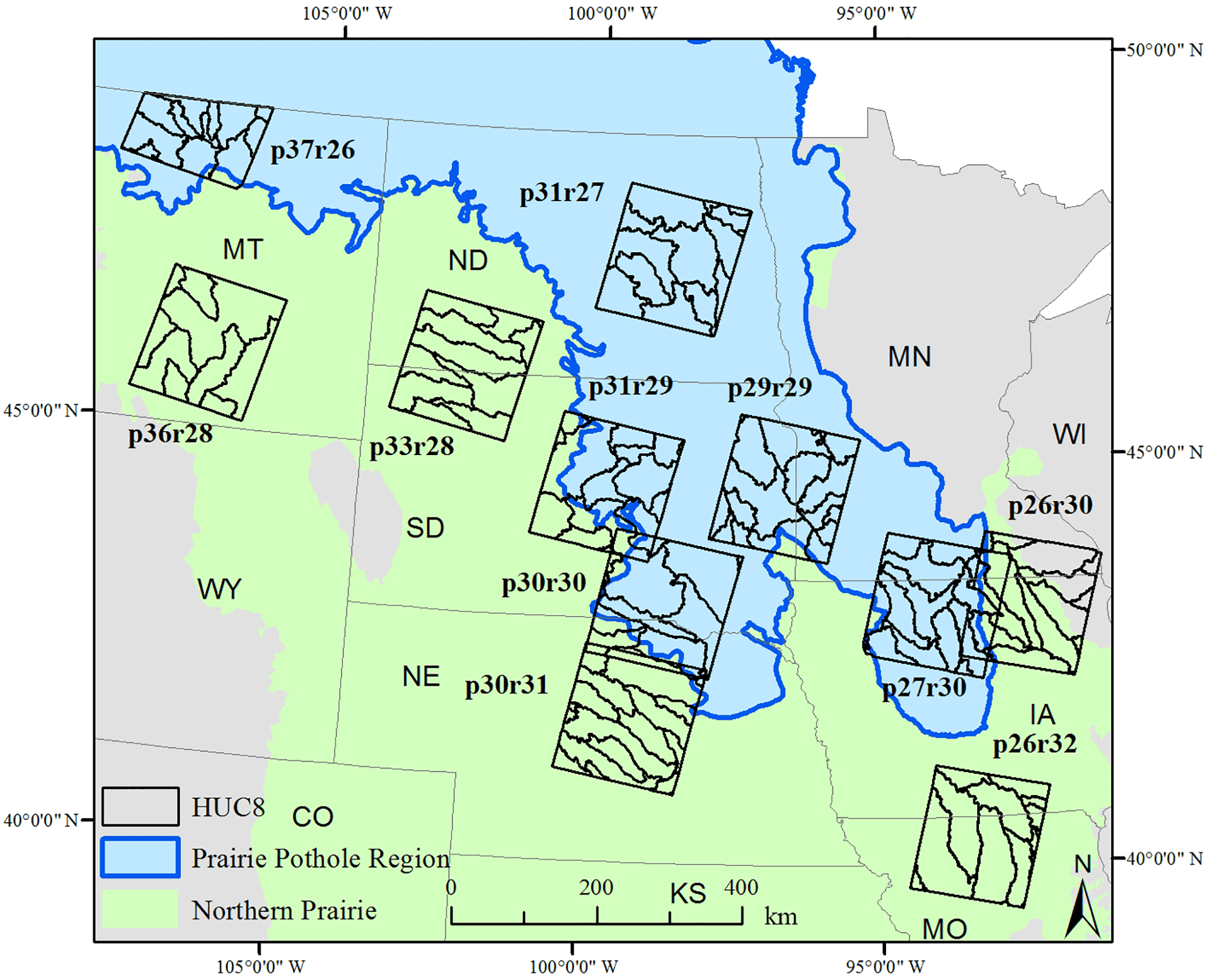
Figure 1 Distribution of Landsat path/rows used to map surface water extent and corresponding eight-digit Hydrological Units (HUC8s) used for further analysis in relation to the boundary of the Prairie Pothole Region (PPR). The p37r26 behaved dissimilarly from the PPR and similarly to the adjacent Northern Prairie (NP) in all regards and was therefore included with the NP for analyses organized by PPR and NP.

2.1 Study area

Our study area consisted of 11 Landsat path/rows (total area = 308 439 km²) in the US portion of the PPR and adjacent NP (Fig. 1). The PPR across North and South Dakota, western Minnesota, northern Iowa, and northern Nebraska, is dominated by the North and Northwest Glaciated Plains. This ecoregion is characterized by landscape features formed during its recent glacial history. Drift plains, large glacial lake basins, and shallow river valleys support row crop agriculture. Grasslands and livestock grazing dominate areas where glaciers left deposits of uneven glacial till (Sayler et al., 2015). The PPR is dominated by cultivated crops (59 %), herbaceous land cover (18 %), and hay/pasture (10 %) (Homer et al., 2015). Adjacent to the PPR, the Northwestern Great Plains, across western North and South Dakota, is a semiarid unglaciated plain which tends to have shallow soils with a clay texture not conducive to growing crops and instead dominated by livestock grazing across grasslands (Sayler et al., 2015). To the southeast of the North Glaciated Plains lies the Western Corn Belt and the Central Irregular Plains in Iowa and Nebraska. Glacial till forms the parent material for most of the soil in Western Corn Belt and the northern part of the Central Irregular Plains, within the study area. Level and gently rolling hills and fertile soils support agriculture (Sayler et al., 2015). The NP is dominated by herbaceous land cover (47%) with cultivated crops (28 %) and hay/pasture (9 %) is also common (Homer et al., 2015). Using the precipitation averages (1981–2010) defined by the Parameter-elevation Regressions on Independent Slopes Model (PRISM, Daly et al., 2008), the PPR study area receives 6 % more precipitation on average than the NP study area (626 mm yr⁻¹ relative to 592 mm yr⁻¹, respectively) and 1.5 % less evaporative demand or potential evapotranspiration (PET) (603 mm yr⁻¹ relative to 594 mm yr⁻1, respectively). These differences were not found to be statistically different using the Wilcoxon rank sum test.

Our regression analysis used eight-digit Hydrologic Unit Codes (HUC8s; USDA NRCS, 2015) as the unit of analysis (n = 150) across all 11 Landsat path/rows (Fig. 1). HUC8s were used instead of smaller watersheds such as HUC10s or HUC12s to ensure that patterns in surface water expansion and contraction represented landscape patterns, not individual or small groups of water features. HUC8s that occurred at the edge of a Landsat path/row with an area of < 50 ha were excluded from further regression analysis to limit the inclusion of incompletely characterized watersheds. The threshold of 50 ha was selected as it was a natural break in the distribution of HUC8 sizes. Patterns of surface water expansion and contraction were compared between the PPR and NP. We note that one path/row (p37r26) in northern Montana was technically within the western most section of the PPR, but was found to behave dissimilarly from the PPR and similarly to the NP in terms of both its landscape characteristics (e.g., stream density, wetland density) and surface water expansion and contraction. Because of this, p37r26 was included in the adjacent NP for analyses where findings were organized by PPR and NP.

2.2 Landsat image processing

2.2.1 Path-row and image selection

surface water extent was mapped for a series of images across 11 Landsat path/rows (Fig. 1). These path/rows were selected to represent the PPR and adjacent NP and were intentionally selected to represent a range of ecoregions, climate conditions (west to east and north to south), and densities of wetlands and streams. Snow-free images (acquired from approximately April through October) containing less than 10 % cloud cover from the Landsat 4–5 TM, Landsat 7 ETM+ (prior to failure of the scan-line corrector in 2003) and Landsat 8 OLI sensors were selected between 1985 and 2015. The number of images processed within each path/row averaged 14 (range: 9 to 17 acceptable images) and were intentionally selected to document interannual variability in surface water extent, by selecting images from wet, average, and dry years (Table 1). The terms “wet”, “average”, and “dry” were defined in reference to local norms, using the Palmer Hydrological Drought Index (PHDI) and the 12-month Standardized Precipitation Index (SP12) (NOAA NCDC, 2014). The range of conditions captured by the time series within each path/row in relation to the historical climate conditions (1895–2015) are shown in Table 1. The PHDI is based on a monthly water balance accounting approach that considers precipitation, evapotranspiration, runoff, and soil moisture. The indices rely on weather station data and are interpolated at 5 km (NOAA NCDC, 2014). A complete list of images included in the analysis is presented in the Appendix (Table A1).

Table 1 A summary of the Landsat images utilized within each selected path/row. Landsat TM images were used for dates 2011 and earlier. Landsat 8 OLI images were used for 2013 forward. DOY – day of year; NP – Northern Prairie, PPR – Prairie Pothole Region, and PHDI – Palmer Hydrological Drought Index. ^* p37r26 was considered NP because of its dissimilarity with the rest of the PPR.

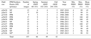
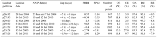
Table 2 Landsat images and corresponding National Agricultural Imagery Program (NAIP) images used to validate the Landsat surface water extent maps. Accuracy is presented here by Landsat image. PHDI – Palmer Hydrological Drought Index, SP12 – 12-month Standardized Precipitation Index, OE – omission error for water, CE – commission error for water, OA – overall accuracy, DC – Dice coefficient, and RB – relative bias.

2.2.2 Image processing

Images were atmospherically corrected and converted to surface reflectance values using the Landsat Ecosystem Disturbance Adaptive Processing System (Masek et al., 2006). A minimum noise fraction transformation was applied to reduce within-image noise (Green et al., 1988). The per-pixel water fraction was estimated using the Matched Filtering algorithm, a partial unmixing method in the ENVI software package (Exelis Visual Information Solutions, Inc, Herndon, Va) (Turin, 1960; Vanderhoof et al., 2016). This algorithm is trained on a water spectral signature, which was derived from open-water polygons manually selected within each path/row, resulting in a water signature specific to each image. Three to four polygons (minimum size of 1 ha per polygon, total training area per path/row was approximately 20 ha) per path/row were selected. The same open-water polygons were used to train the time series for each path/row. The water fraction output was linearly stretched to maximize our ability to separate water from non-water. CFmask, a quality-control layer provided with Landsat images, was used to mask out clouds and cloud shadows (Zhu and Woodcock, 2014), while the National Land Cover Database (NLCD) was used to mask out impervious surfaces, defined as low, medium, and high-density development (Homer et al., 2015), which can show spectral confusion with surface water. Each surface water image was visually inspected for quality using visual interpretation as well as ancillary datasets (e.g., National Agricultural Imagery Program – NAIP – imagery, National Wetlands Inventory – NWI – dataset; USFWS, 2010). Select images were removed or edited primarily due to spectral confusion between water and bare rock or shadowed vegetation.

2.2.3 Surface water extent validation

The surface water extent maps were validated using 1 m resolution NAIP imagery. Landsat images were selected for validation based on the temporal coincidence of the Landsat and NAIP imagery collections (Table 2). Because terrestrial surface water is a relatively rare cover type, it is difficult to generate enough inundated reference points through a simple random-point generation. Therefore, random points were generated in reference to NWI polygons overlapping with the NAIP and Landsat imagery. Points were then visually identified as inundated or non-inundated using the NAIP imagery. To account for the scale difference between a random point and a 900 m² Landsat pixel, the Landsat pixel boundaries for each random point were identified. The point was classified as the majority class (inundated or non-inundated) identified by NAIP within the Landsat pixel boundary surrounding each random point. Reference points were generated per Landsat/NAIP pair (500 or 1000), with the number of reference points varying depending on the amount of NAIP imagery available within the Landsat path/row extent, and the number of random points that occurred within Landsat NA pixels. Metrics presented included overall accuracy, omission error, commission error, dice coefficient, and relative bias. Omission and commission errors were calculated for the category “water”. The dice coefficient is the conditional probability that if one classifier (product or reference data) identifies a pixel as water, the other one will as well, and therefore integrates omission and commission errors (Fleiss, 1981; Forbes, 1995). The relative bias provides the proportion that water is underestimated (negative) or overestimated (positive).

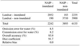
The Landsat per-pixel fraction water was binned into inundated (≥ 0.3) and non-inundated (< 0.3) classes. This threshold was selected as it best balanced errors of omission and commission. Overall accuracy for the Landsat surface water maps across the 11 path/rows was 93.9 % with errors of omission for surface water averaging 8.5 % and errors of commission for surface water averaging 8.2 % (Table 3). Errors of commission were higher for p33r28 which can be attributed to confusion in agricultural fields and with bare rock formations. The surface water maps showed no relative bias and a dice coefficient of 92 %. To determine the minimum wetland size that was reliably detected, we randomly selected 400 NWI wetlands (from < 0.1 to 1.0 ha) visibly inundated in the NAIP imagery (Table 2). Wetlands larger than 0.2 ha were reliably detected by the Landsat surface water maps (73 %). Errors of omission and commission can be primarily attributed to mixed Landsat pixels occurring over small wetlands (a few pixels in size) or at the edge of larger wetlands or open water features. In some images, parts of or entire agricultural fields were classified as water. It is common in both the spring months, when crops need to be planted, and fall months, when crops are being harvested, for fields to experience wet conditions (Fausey et al., 1987; King et al., 2014). In addition, poorly drained soil is common across this region (Skaggs et al., 1994) and wetland depressions often occur within agricultural fields. Consequently, subsurface tile drainage has become increasingly popular across the region to speed up the removal of excess soil water (Blann et al., 2009). It is often unclear to what extent surface water mapped within agricultural fields represents historical or current wetlands, poorly drained fields, or misclassified pixels. Lastly, a close match in acquisition date between the Landsat and NAIP images is essential for the NAIP imagery to accurately represent ground conditions. Variability in the date match can be considered one potential source of error, as the occurrence of a rain event or seasonal variability can change surface water conditions over even short time periods.

2.3 Surface water extent analysis

surface water abundance (ha km⁻²) was calculated per HUC8 with HUC8 area being adjusted for each image based on the abundance of not applicable (n/a) pixels (e.g., cloud cover, cloud shadow) in each image. We used the high-resolution National Hydrography Dataset (NHD, 1 : 24 000) to classify surface water as (1) continuous connected with the stream network, or (2) disconnected from the stream network. The NHD line dataset was buffered by 14 m, the reported digital horizontal accuracy of the dataset (USGS, 2010) and NHD area was added to account for the width of large rivers. surface water polygons that intersected the stream network in a given image were classified as continuously connected water (CCW). surface water polygons that did not intersect the stream network in a given image were classified as discontinuous water (DCW) or discontinuous from the stream network. We acknowledge that the NHD is known to be incomplete (e.g., lacking short and ephemeral stream lines) and that some stream lines within the NHD are disconnected from downstream waters (Heine et al., 2004). However, the NHD is the most complete nationally available stream dataset.

Table 3 Summary of accuracy statistics across all of the Landsat images validated using National Agricultural Imagery Program (NAIP) imagery.

Processed images within each path/row were ranked from least-to-most amount of surface water per area. Median condition was defined as the image or two images representing the median amount of surface water extent, estimated from all images within a path/row. Drought and deluge conditions were defined as the average of the two end-member images showing the least and most amount of total surface water extent for each path/row, respectively. surface water extent was then summed across the PPR and NP path/rows and divided by the total area to calculate the hectares of surface water extent per km² for each region. The NP portion of path 27, row 30 (p27r30) and p30r30 were deleted, as was the PPR portion of p26r30 to avoid double-counting overlapped path/rows. The NP and PPR portions of p31r29 were analyzed separately.

2.4 Stage 1 – derivation of the Surface Water Climate Response (SWCR)

In stage 1, surface water extent in each HUC8 was related, using linear regression, to water availability, defined as precipitation minus PET summed over a time interval. Water availability provided an estimate of the amount of water in each watershed available to either (1) runoff, (2) infiltrate to shallow or deep groundwater sources, or (3) be stored as surface water. Surface water was again partitioned into CCW and DCW using its spatial relationship to the NHD. Precipitation data were compiled using the Parameter-elevation Regressions on Independent Slopes Model (PRISM, Daly et al., 2008). PET, or the atmospheric demand for evaporation and transpiration in the absence of water limitations, which can be expected over open surface water, was compiled using gridded surface meteorological data PRISM and the North American Land Data Assimilation System Phase 2 (Abatzoglou, 2011). PET was calculated using the Penman–Monteith equation that required inputs of minimum and maximum temperature, daily average dew point temperature (equivalently, vapor pressure or vapor pressure deficit), wind speed and downward shortwave radiation (Abatzoglou, 2011; Mitchel et al., 2004). The datasets were resampled to 125 m using cubic convolution and summarized for each HUC8. Water availability was summed for a series of monthly periods preceding each image date (3, 6, 9, 12, 18, 24, 30, and 36 months) to identify the accumulation period for which the greatest number of HUC8s showed a significant (p < 0.05) slope between water availability and surface water extent. This logic was meant to reduce the probability that a zero slope resulted from surface water responding more strongly to climate drivers at a different time interval. This first stage produced surface water climate response (SWCR), our dependent variables for stage 2, i.e., the slope of the relationship between CCW and DCW surface water extent to accumulated water availability (Fig. 2). The slope or stage 2 dependent variable is referred to as the surface water climate response (SWCR) from this point forward.

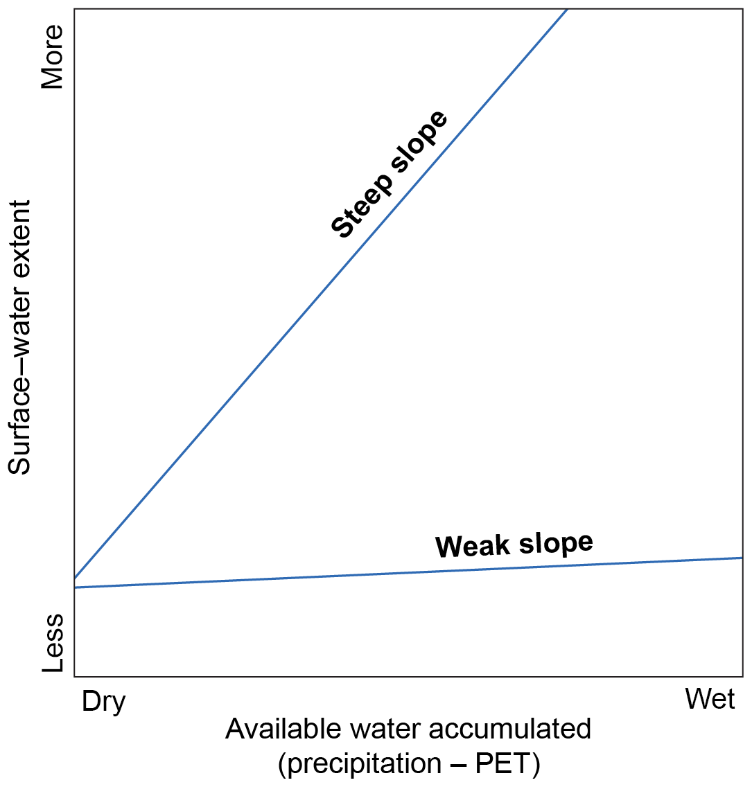
Figure 2 Theoretical figure showing the derived dependent variable, or the Surface Water Climate Response (SWCR), defined as the slope of the statistical relationship between accumulated water and surface water extent. Some areas show a greater SWCR or substantial increase in surface water extent as more water becomes available via precipitation minus potential evapotranspiration (PET), while other areas show little to no change in surface water extent, presumably as excess water leaves the system through runoff or infiltration.

Cloud cover makes it challenging to restrict analysis of Landsat imagery to a specific season, while including imagery that covers more than one season potentially conflates seasonal surface water dynamics with interannual surface water dynamics. The influence of seasonal change in surface water extent within our analysis contributed to the uncertainty (primarily through sampling error) in the SWCR. For example, if we included an image from June 1993 and one from August 1993 and related both images to the last nine months of precipitation and PET (September 1992–May 1993 and November 1992–July 1993, respectively), greater seasonal dynamics or variation in surface water extent between the two dates can be expected to show up as greater uncertainty in the slope, defined by the standard error of the slope or standard error of the SWCR. This becomes more evident as the accumulated period becomes larger (e.g., 36 months). By explicitly considering the uncertainty of the SWCR in the regression analysis, as described below in the stage 2 analysis (Sect. 2.6), we can, to the extent possible, account for seasonally induced variation in surface water extent.

2.5 Landscape variables for stage 2 analysis

The independent variables summarized for each HUC8 and included in the analysis were selected to characterize mechanisms through which water can leave the landscape (e.g., infiltration, runoff, tile drainage), mechanisms through which water can remain and expand on the landscape (e.g., wetland density, wetland size, topography), as well as other potential influences on surface water dynamics (e.g., climate norms, land cover). The NWI (USFWS, 2010) and NHD stream dataset (USGS, 2013) were used to calculate wetland and stream characteristics including stream density, wetland count and areal density, and proportion of total wetland area attributed to large (> 8 ha) features. A threshold of 8 ha was selected as this is the size threshold used by USFWS to define a lacustrine system (Cowardin et al., 1979). We do not refer to these features as lakes, however, as water depth and associated vegetation are also important features to defining lacustrine systems, and were not evaluated. We did not include distance variables, which were previously found to be highly correlated with simpler variables already in the analyses: mean wetland-to-wetland distance was previously found to be highly correlated with wetland density (r = −0.95, p < 0.01) and mean wetland-to-stream distance highly correlated with stream density (r = 0.88, p < 0.01) (Vanderhoof et al., 2017). We included the proportion (%) DCW was of total surface water as a proxy of the relative distribution of water storage across the watershed between riparian and non-riparian water bodies. Surface topography can influence the capacity for surface water to expand and was quantified as the weighted averaged slope gradient, as defined by the US Department of Agriculture's Soil Survey Geographic (SSURGO) database (Soil Survey Staff, 2017). Topographic Wetness Index was not included because of the relative weakness of such indices in landscapes with little relief (e.g., Schmidt and Persson, 2003) and the data intensive nature of calculating TWI with a 10 m digital elevation model (DEM) across such a large study area. Additional variables derived from the SSURGO database to characterize infiltration capacity include available water storage (0–150 cm), annual minimum depth to water table, and saturated hydraulic conductivity (K_sat). Human influence was quantified as the abundance of agricultural activities, or the percent of each HUC8 classified as agriculture, defined as the National Land Cover Database (NLCD; Homer et al., 2015) cover categories hay/pasture and row crop. Anthropogenic modifications to drainage systems, or the percent land cover artificially drained, was estimated as the percent of each HUC8 where row crop cover type (NLCD) and very poorly drained or poorly drained soils as defined by the National Resources Conservation Service's SSURGO database were collocated following Christensen et al. (2013). The climate normals per HUC8 (1989–2013) were calculated to represent the Landsat image range. Multi-decadal climate normals were included to test for the potential effect of a climate gradient across the study area. The precipitation averages are provided as part of the PRISM dataset (Daly et al., 2008). PET was calculated as a function of monthly mean PRISM temperature and day length following Hamon (1961). The Moisture Index (MI) was calculated as the ratio of precipitation and PET where, if PET exceeded precipitation, MI = precipitation/PET − 1, and if precipitation exceeded or equaled PET, then MI = 1 = PET/precipitation. Values range from −1 (dry) to 1 (wet) (Willmott and Feddema, 1992; Feddema, 2005). The climate averages were resampled to 1 km from 4 km using inverse-distance weighting, prior to being averaged per HUC8. The distribution of values within each of the independent variables is shown in Table 4. Spearman rank correlations with a Bonferroni correction (Dunn, 1961) were calculated for the independent variables (Table A2).

Table 4 Independent variables considered in the landscape analysis and the distribution of values for each variable across the 8-digit hydrological units (HUC8s). Mean values for the HUC8s within the Prairie Pothole Region (PPR) and Northern Prairie (NP) are also shown with significant differences (p < 0.01) between the two groups, as determined by the Wilcoxon rank sum test, indicated by different superscript letters. NHD – National Hydrography Dataset, NWI – National Wetlands Inventory, PRISM – Parameter-elevation Regressions on Independent Slopes Model, SSURGO – Soil Survey Geographic Database, NLCD – National Land Cover Database, DCW – disconnected surface water, PET – potential evapotranspiration, avg – average, and K_sat – saturated hydraulic conductivity.

2.6 Stage 2 – analysis – landscape mechanisms explaining variability in SWCR

In stage 2, CCW and DCW SWCRs, or the slope of the relationship between CCW and DCW and accumulated water availability, were related to landscape variables using feasible generalized least-squares (FGLS) regression, with HUC8s (n = 150) as the unit of analysis. FGLS allowed us to estimate the heteroscedastic structure of the residuals (Lewis and Linzer, 2005) and has been previously applied within landscape ecology contexts (e.g., Acharya, 2000; Villalobos-Jimenez and Hassall, 2017). The SWCRs were found to be significant for the largest number of HUC8s using a 9-month period of accumulation for both CCW and DCW, which was therefore used as the accumulation period for further analyses (Table 5). The SWCRs were found to be spatially autocorrelated using Global Moran's I (spatial relationship conceptualized using inverse distance) (DCW SWCR, 9 months, z-score = 7.8, p < 0.01, CCW SWCR, 9 month, z-score = 4.1, p < 0.01), violating the assumption of independence between samples. To account for spatial autocorrelation in the SWCRs, we calculated an autocovariate in ArcGIS 10.3, Geostatistical Analyst (ESRI, Redmond CA) which uses adjacent HUC8s to create a neighbor value. By including a spatial autocovariate in the ordinary least-squares (OLS) regression model, we controlled for how much the response variable reflected response values of adjacent HUCs, before identifying additional significant explanatory variables (Dormann et al., 2007; Betts et al., 2009). The autocovariate was automatically retained while only significant independent variables (p < 0.05) were additionally retained. The dependent variable was normalized using a Box–Cox power transformation (R package MASS, Venables and Ripley, 2002). Multicollinearity was formally assessed using the regression collinearity diagnostics described by Belsley et al. (1980) and implemented in the R package perturb (Hendrickx, 2012). Collinearity may affect parameter estimation when a condition index greater than 10 is associated with variance decomposition proportions greater than 0.5 for two or more explanatory variables (Belsley, 1991). Both models complied with collinearity requirements.

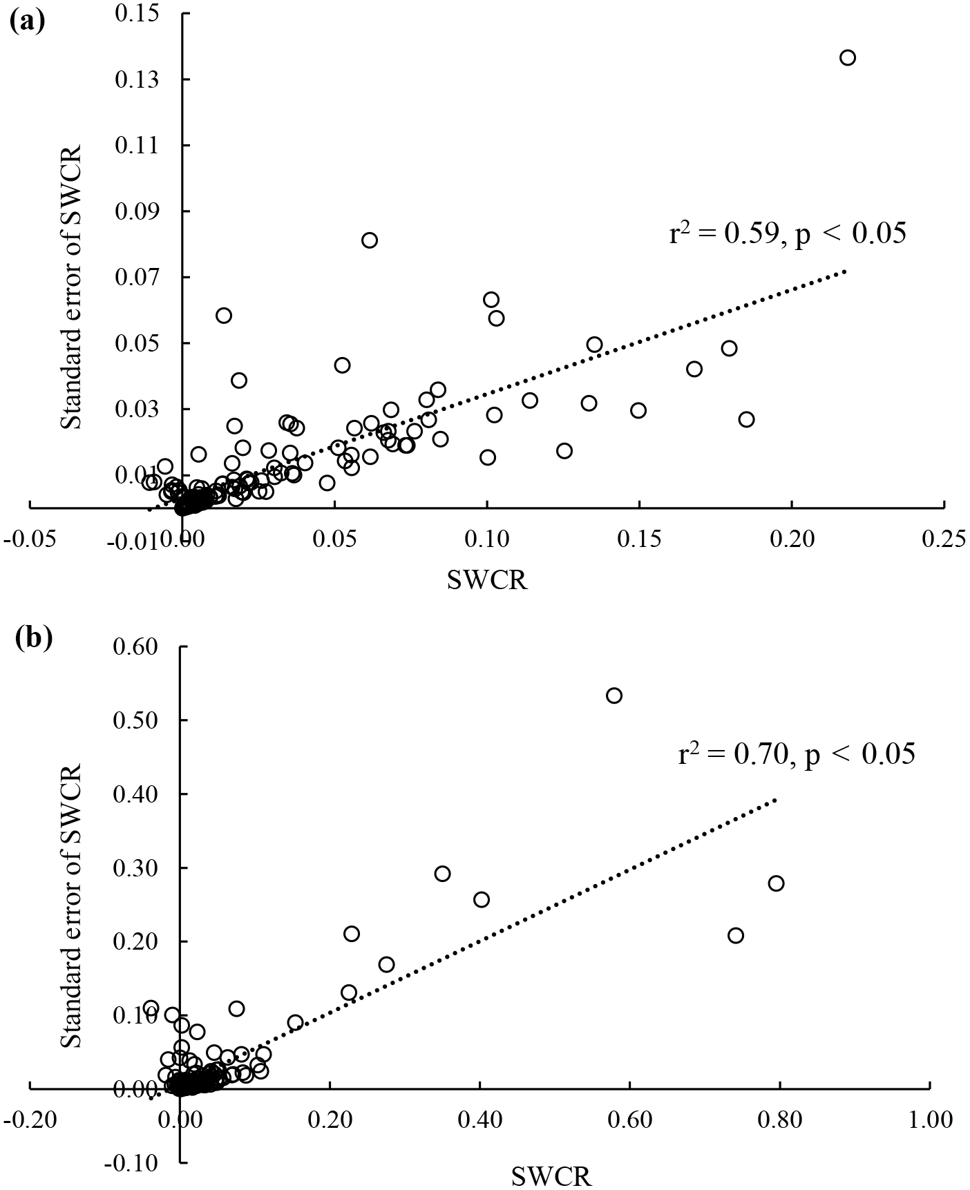
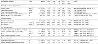
Figure 3 Standard errors of the Surface Water Climate Response (SWCR) tended to be positively correlated with both (a) discontinuous surface water (DCW) or surface water disconnected from the stream network and (b) continuously connected water (CCW) or surface water connected to the stream network.

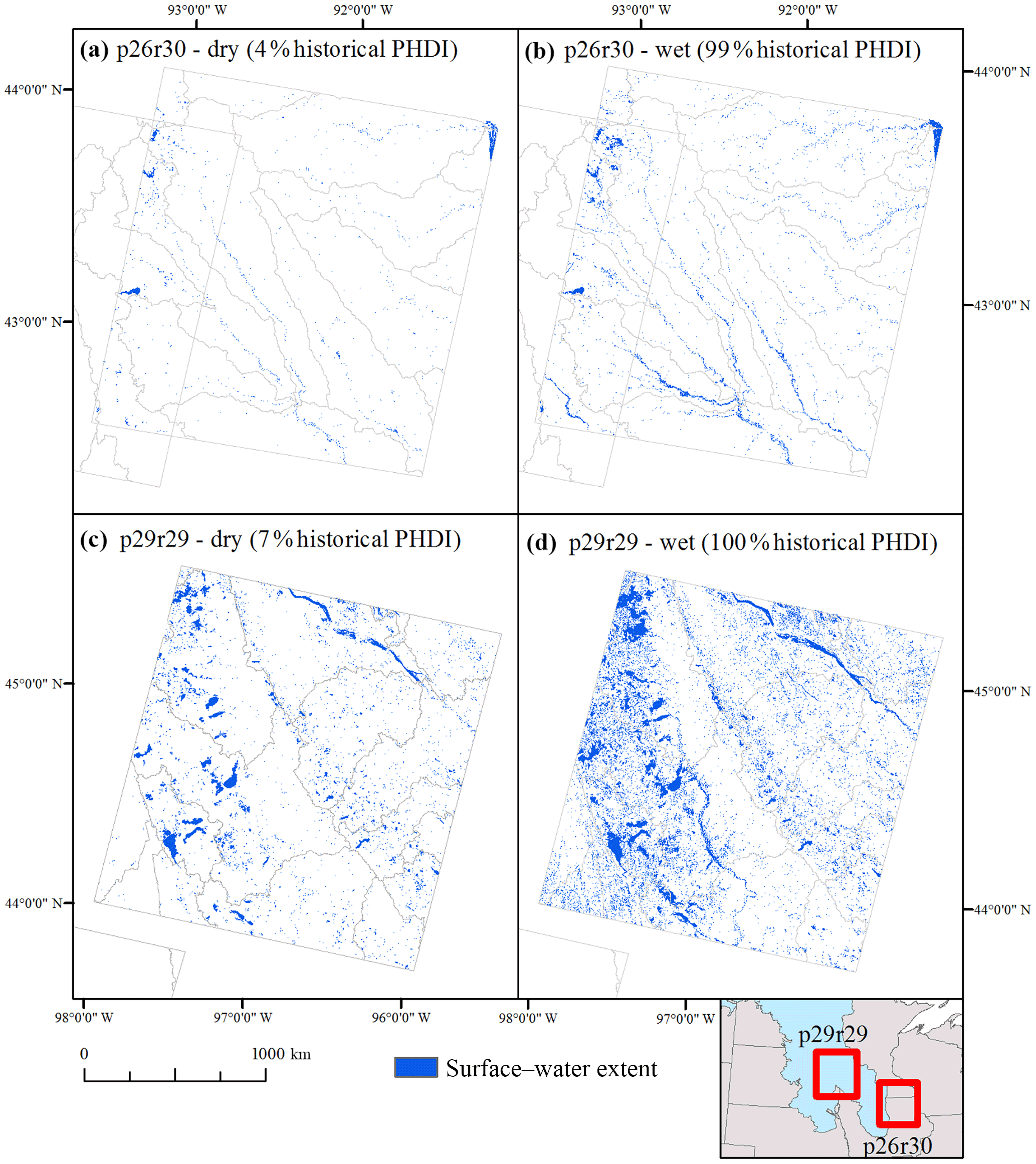
Figure 4 Mean surface water abundance and the amount of “wetting up” varied substantially between different Landsat path/rows. Portions of the Northern Prairie (e.g., p26r30) showed relatively less surface water extent and expansion (a, b) while portions of the Prairie Pothole Region (e.g., p29r29) showed relatively more surface water extent and expansion (c, d). Note: not all water is visible at this reduced scale. PHDI – Palmer Hydrological Drought Index.

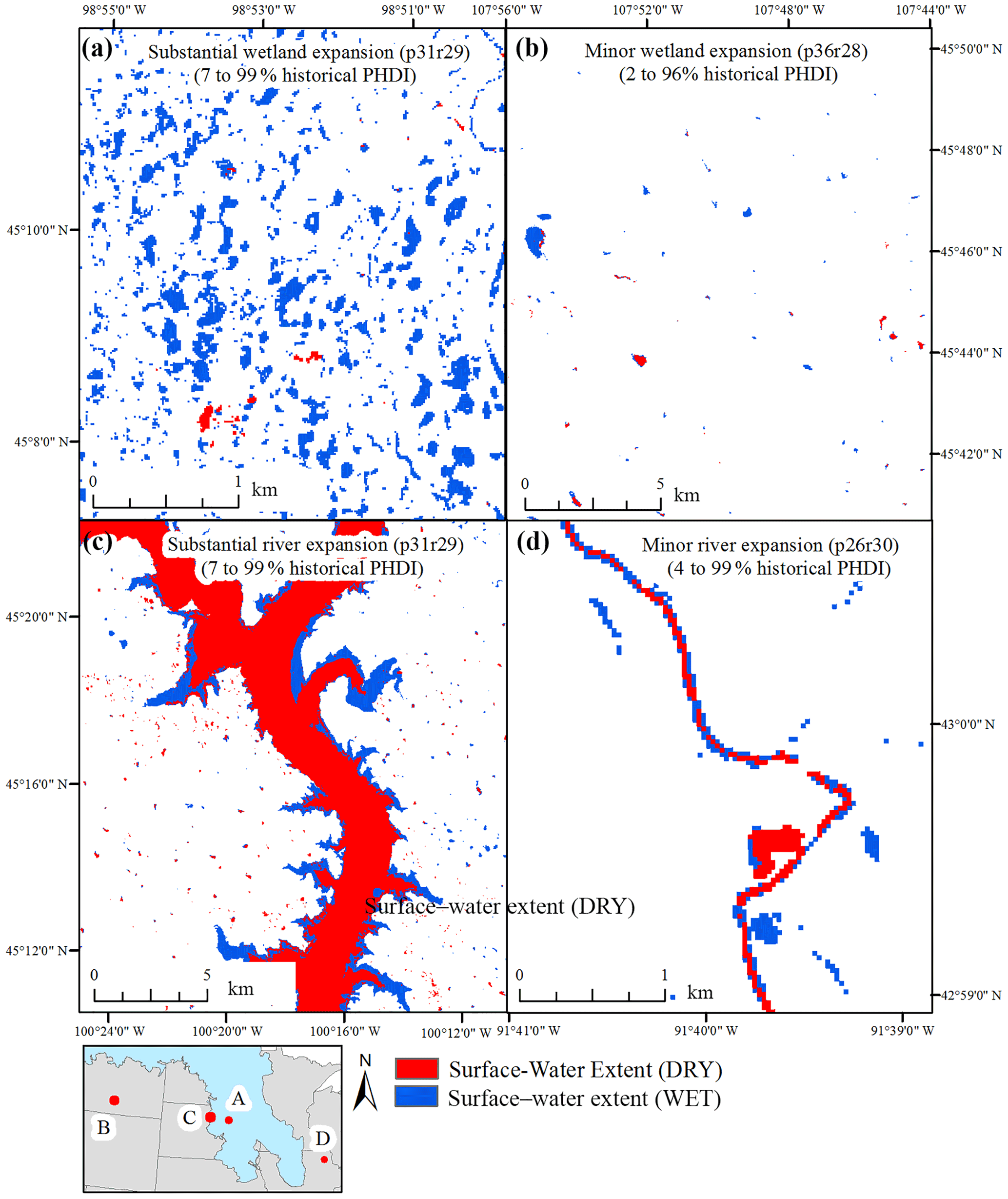
Figure 5 Examples of minor and substantial expansion of surface water extent between historically dry and historically wet points in time. PHDI – Palmer Hydrological Drought Index.

Having an estimated dependent variable (e.g., SWCR) does not necessarily present a problem for a regression analysis, but we must recognize that the regression model error term contains two components: (1) the expected random error resulting from sources of variation not taken into account in the model, and (2) the difference between the true value of the dependent variable and the estimated value (sampling error). In this study, the uncertainty around the dependent variable (SWCR) was not constant across observations. Instead, the dependent variable showed a strong positive correlation with its standard error (DCW SWCR, R² = 0.59, p < 0.05; CCW SWCR, R² = 0.70, p < 0.05) (Fig. 3). FGLS allowed us to estimate both components of the error. To do so we: (1) calculated the logarithm of squared residuals from the OLS model; (2) regressed the log-residuals on the independent variables included in the OLS model; (3) calculated the exponential of fitted values from that regression, which estimates the variance of the regression residual that is not due to sampling of the dependent variable, z; and (4) estimated the basic model again now including weights (1 z⁻¹) (Hanushek, 1974; Lewis and Linzer, 2005). We found the final model residuals to be random using the studentized Breusch–Pagan test (Breusch and Pagan, 1979).

To help add confidence regarding which landscape variables were more or less important, we also fit random forest models in R using the package randomForest (Liaw and Wiener, 2005). The random forests were run with the SWCRs as the dependent variable and landscape characteristics as independent variables. We derived 500 binary trees or bootstrap iterations using out of bag (OOB) samples (70 % of samples to train and 30 % of samples to validate). Variable importance was calculated as the change in node impurity (i.e., Gini importance). Random forest models are generally insensitive to collinearity among metrics; however, the inclusion of correlated variables can deflate variable importance as well as the overall variation explained by the model (Murphy et al., 2010). We implemented random forest model selection to select the smallest number of non-redundant variables (varSelRF R package) (Murphy et al., 2010).

3 Results

3.1 Surface water extent

Median surface water extent as well as the amount of water added and lost from the surface between wet and dry periods was found to vary considerably across the study area (Figs. 4 and 5). Analysis of the median total surface water extent between the PPR and the NP demonstrated that the PPR had 2.6 times greater surface water extent than the NP (Table 6). The PPR also showed greater variability in total surface water extent, adding 5.7 ha km⁻² during very wet conditions and losing 2.8 ha km⁻² during very dry conditions, for a maximum net difference of 8 ha km⁻². This can be compared to the NP which gained 1.6 ha km⁻² during very wet conditions and lost 0.8 ha km⁻² during very dry conditions, a net difference of 2.4 ha km⁻² (Table 6). DCW, or water that was discontinuous with the stream network, showed greater expansion and contraction in extent in both the PPR and NP, relative to CCW which intersected the stream network. Consequently, DCW increased as a percent of total surface water during wet periods and decreased as a percent of total surface water in dry periods. This suggests that across the study area, surface water that was disconnected from the stream network disproportionately served a surface water storage function during wet periods, reducing the amount of water contributing to downstream flooding. Similarly, DCWs disproportionately experienced loss during dry periods.

3.2 Relationship between surface water extent and water availability

Including PET instead of using precipitation alone tended to increase the percentage of HUC8s showing a statistically significant relationship between surface water extent and water availability across the different accumulation periods that we tested, although this was not true for all time periods. For instance, the percent change from precipitation to precipitation minus PET ranged from −1.4 to 38 % for DCW and −6.3 to 24.3 % for CCW. For DCW there was a jump in the percentage of HUC8s showing a significant relationship between six and nine months, but the percentage of HUC8s stabilized after this time period out to 36 months. CCW showed a similar but smaller jump in the percentage of HUC8s with a significant relationship between six and nine months (Table 5). At nine months, all images, regardless of being collected in the spring, summer or fall, would include winter precipitation. We observed substantial spatial variability in the statistical relationship between surface water extent and water availability. Using nine months as the accumulation period, we observed a strong spatial pattern in DCW. PPR HUC8s tended to show a greater SWCR, exhibited by a substantial increase in surface water extent with increased water availability, while HUC8s across the NP tended to show a smaller SWCR, exhibited by minor to no increases in surface water extent with increased water availability (Figs. 6 and 7). For CCW, the spatial pattern was less consistent within the PPR or ecoregion boundaries. Instead, HUC8s with a greater SWCR tended to be HUC8s with large lakes or floodplains (Figs. 6 and 7).

3.3 Landscape variables explaining variability in surface water response

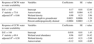
For DCW SWCR, when independent variables were assessed individually using Spearman's rank correlation, the SWCR was greater in locations with fewer streams (R = −0.64, p < 0.05), lower slope gradient (R = −0.59, p < 0.05), higher wetland density (R = 0.52, p < 0.05) and total wetland area (R = 0.51, p < 0.05), deeper minimum depth to water table (R = 0.59, p < 0.05), and where a greater proportion (%) of the total surface water was disconnected from the stream network (R = 0.42, p < 0.05) (Table 7). When the relative importance of the variables was tested using random forest, variables found to be the most important included, wetland density, stream density, annual minimum depth to water table, and the slope gradient (Table 7). However, after accounting for the spatial autocorrelation in the DCW SWCR and the significance of the variables, the DCW SWCR increased in the final feasible generalized least-squares model (adjusted R² = 0.66, F statistic = 73.6) with (1) greater wetland density, (2) deeper depth to groundwater, and (3) less anthropogenic drainage (Table 8). The variable most consistently identified across statistical approaches was wetland density, the relevance of which is demonstrated in Fig. 5a and b.

For CCW SWCR, fewer independent variables showed a significant Spearman rank correlation. The SWCR for stream-connected water increased in locations with a greater total wetland area (R = 0.48, p < 0.05) and less average precipitation (R = −0.33, p < 0.05) (Table 7). Using random forest, the total wetland area and proportion of total water from large features were found to be the most important variables in explaining variation. The final feasible generalized least-squares model (adjusted R² = 0.54, F statistic = 37.4) also found the relationship between CCW and surface water availability (i.e., SWCR) was stronger with greater total wetland area, but also found that it decreased with greater wetland density (Table 8).

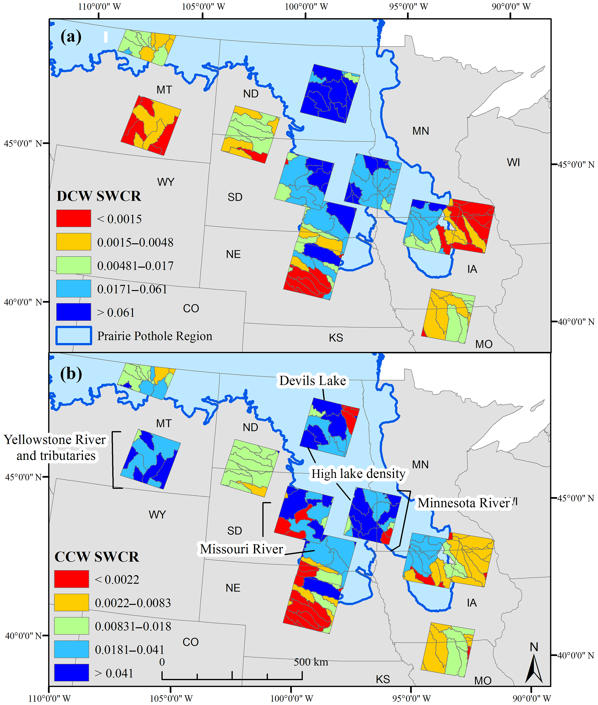
Figure 6 The spatial distribution of the Surface Water Climate Response (SWCR) values from the statistical relationships between available water, defined as precipitation minus potential evapotranspiration accumulated over the previous nine months, and surface water extent. Greater SWCR values indicate greater change in surface water extent with increased available water. Surface water extent was divided between (a) disconnected surface water (DCW), or surface water extent disconnected from the stream network, and (b) continuously connected water (CCW), or surface water extent connected to the stream network.

Table 5 The percent of HUC8s across the study area that showed a significant relationship (p < 0.05) between surface water extent and (1) precipitation (Precip or P) or (2) precipitation minus potential evapotranspiration (PET) for different accumulation periods. DCW – disconnected surface water; CCW – continuously, connected surface water.

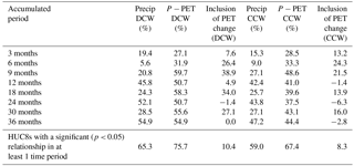
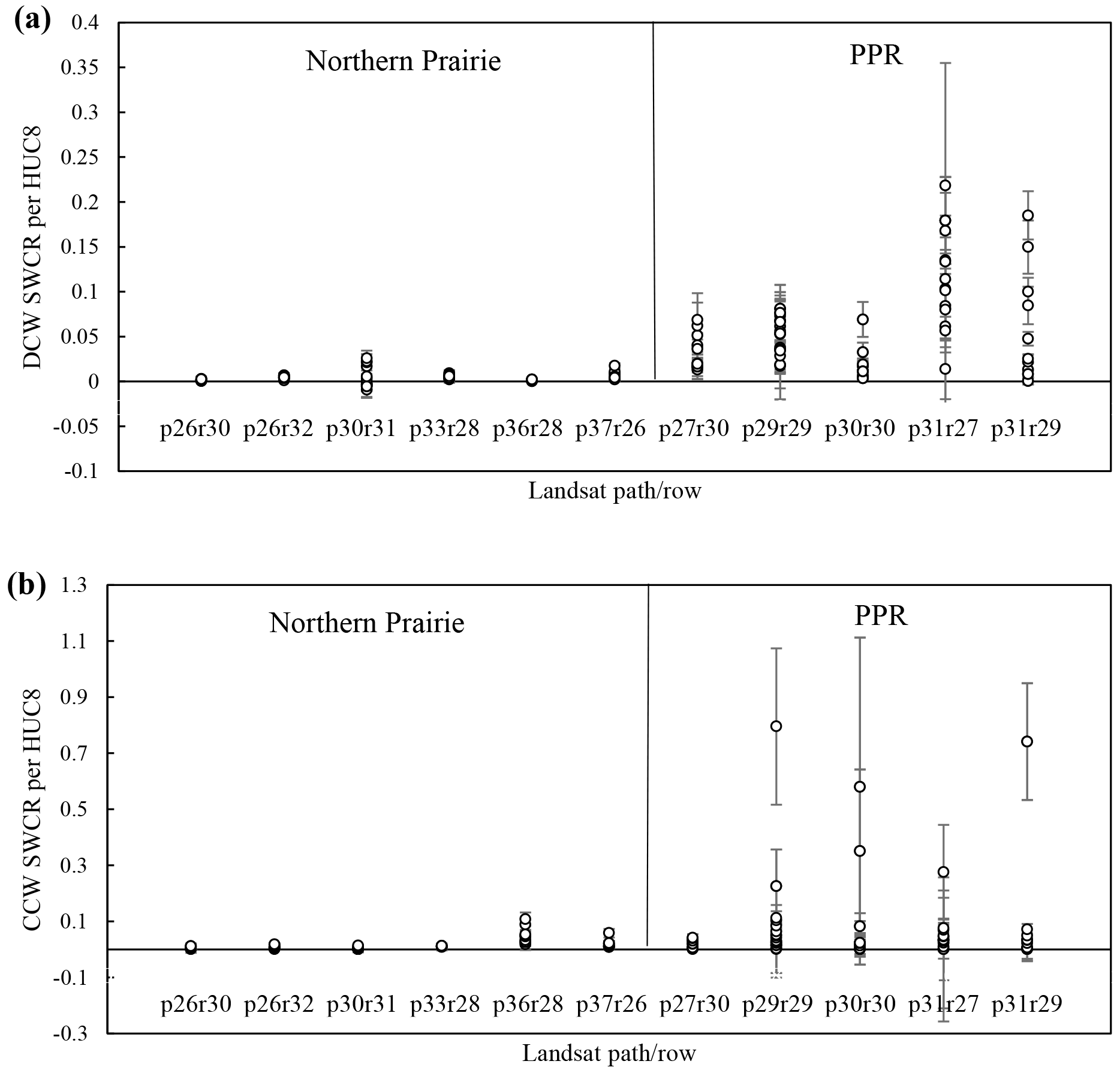
Figure 7 Distribution of Surface Water Climate Response and standard error values organized by Landsat path/row and primary path/row location, i.e., the Northern Prairie or the Prairie Pothole Region (PPR) for (a) surface water that is disconnected from the stream network (DCW), and (b) surface water that is connected to the stream network (CCW). HUC8 – eight-digit Hydrological Units.

Table 6 Surface water extent conditions summarized for the Prairie Pothole Region (PPR) and adjacent Northern Prairie (NP). TSW – total surface water extent, CCW – continuously connected surface water that intersects the stream network, and DCW – disconnected surface water or surface water that does not directly intersect the stream network.

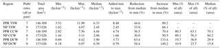
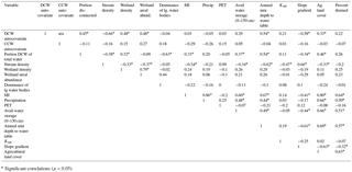
Table 7 Spearman rank correlation values between the dependent variables and each of the independent variables considered in the analysis. Bonferroni correction was applied to the p values and significant correlations (p < 0.05) are starred. Relative variable importance as determined by random forest models are also presented for each variable (i.e., increase in node purity). PET – potential evapotranspiration, K_sat – saturated hydraulic conductivity, DCW – disconnected surface water, and CCW – continuously, connected surface water.

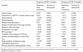
¹ Variables selected by the random forest model selection process, using the R package rfUtilities, when the autocovariate was not included. ^* Significant correlations (p < 0.05).

Table 8 Feasible generalized least square models with residual weights applied relating the response (of surface water extent to water availability) to landscape-related variables. All variables included in the models were significant. DCW – surface water disconnected from the stream network, CCW – continuously connected surface water, SE – standard error, and D.F. – degrees of freedom.

4 Discussion

Surface water extent, and in particular surface water within well-studied portions of the PPR, has been previously shown to exhibit seasonal and interannual patterns (Poff et al., 1997; Beeri and Phillips, 2007; Vanderhoof et al., 2016) that can, in turn, influence the cumulative hydrologic response of a watershed (Evenson et al., 2016; Golden et al., 2016; Ameli and Creed, 2017). What has been less studied is how surface water dynamics vary across diverse landscapes. This is particularly relevant when we consider the need for communities and local agencies to plan ahead for expected changes in the precipitation regime associated with climate change (Dore, 2005; Johnson et al., 2005; Millett et al., 2009; McKenna et al., 2017).

Our study area was intentionally selected to encompass a large area with a wide range of landscape conditions in regards to wetland and stream density and capacity for infiltration. Across the study area, variation in the values of many of the variables (e.g., stream density, wetland density) can be attributed to landscape age or the time since the last glacial retreat, and corresponding variability in drainage development across the region (Ahnert, 1996). The Wisconsin glacier retreated from the PPR by 11 300 BP, meaning the drainage system is still developing and surface water is being stored in glacially formed depressions (Winter and Rosenberry, 1998; Stokes et al., 2007). In contrast, the landscape to the west and south of the PPR, is much older (> 20 000 BP) with a well-developed drainage network (Clayton and Moran, 1982).

Our results demonstrated that the relationship between surface water extent and water availability (SWCR) is a function of both climate and landscape variables and that the density of depressional wetlands, in particular, played a key explanatory role in the observed landscape response to increased climate inputs. Given our findings, we expect that changes in net precipitation from climate change or other climatic forcings will disproportionately affect surface water extent across the PPR relative to the adjacent NP, and that these effects will be more evident in disconnected wetland systems (DCWs) than in wetlands connected to the river network (CCWs). Surface waters that are disconnected from the stream network showed a larger change in extent in response to wetter conditions in landscapes with higher wetland densities or storage capacity. That is to say that landscapes with a larger number of depressional features were found to show a greater increase in surface water extent in response to a wetter climate, relative to landscapes with fewer depressional features (e.g., Fig. 5a and b).

However, a larger DCW SWCR was observed even after controlling for wetland density, suggesting that landscapes with substantial surface storage (i.e., the PPR) may show other landscape characteristics conducive to the accumulation of DCW, for example, reduced infiltration. Correspondingly, the expansion of disconnected water correlated positively with a greater annual minimum depth to groundwater (Table 8). The low permeability of glacial till across the PPR is indicative of a reduction in infiltration, relative to the NP (Sloan, 1972; Winter and Rosenberry, 1995), and would reduce the potential for increased water table elevations, resulting in a deeper minimum depth to groundwater. With less infiltration, pulses of snowmelt or precipitation in the PPR will instead be transported as overland flow and fill wetlands with available storage.

In addition to wetland density and infiltration capacity, DCW SWCR was also found to be related to anthropogenic drainage. The drainage network across the PPR is increasingly modified with the expansion of ditch networks and tile drainage in association with agricultural activities (McCauley et al., 2015). These changes have accompanied extensive human-induced wetland loss across the region (Millett et al., 2009; Van Meter and Basu, 2015). Ditches, pipes and field tiles on the glacial till can hasten the speed with which water leaves a location and lower the water table through increased water withdrawal (De Laney, 1995; Blann et al., 2009; McCauley et al., 2015). We found in the FGLS model, the expansion of disconnected water was inversely related to the abundance of estimated anthropogenic drainage. Because anthropogenic drainage increases the rate at which water leaves a location, it results in the loss or reduction of landscape-scale functions of wetlands and other natural water storage features in the PPR (McCauley et al., 2015), and shifts the hydrologic behaviors of watersheds towards those more commonly seen in the NP.

When we considered surface waters connected to the stream network, we found that CCWs showed more substantial expansion with increased water availability in landscapes with more concentrated water (i.e., greater total wetland area, but lower wetland density) (e.g., Fig. 5c and d). This finding suggests that the presence of stream-connected lakes within large flat basins may be an important factor influencing surface water expansion. Previous research found lakes within the PPR to be important features that commonly experience extensive surface water expansion, subsuming adjacent wetlands during wet periods (Vanderhoof and Alexander, 2016). These findings suggest that if climate conditions within the US portion of the PPR continue to get wetter, as predicted (e.g., Millett et al., 2009; McKenna et al., 2017), then both small wetland depressions and larger features, such as lakes and floodplains, will both serve critical roles in storing increased inputs of surface water, which could prevent downstream flooding.

We must also consider that we may be missing key landscape variables that could explain variability in the spatial response of surface water extent to climate inputs. For example, major landscape characteristics required for stream-connected surface water to expand include (1) large, stream-connected water bodies such as lakes and (2) hydrologically-connected floodplains. The influence of large water bodies was considered by including total wetland area and the portion of water from larger (> 8 ha) features; however, we did not explicitly consider the presence/absence of active floodplains beyond including stream density as a variable. Floodplain activity typically exhibits strong seasonal patterns; while the goal of our analysis was focused on patterns of surface water extent that occurred on longer-time scales (i.e., interannual variability). Because of this, we excluded two Landsat path/rows from the analysis that were originally included because strong seasonal flooding outweighed interannual patterns in climate as evidenced by a lack of a relationship between climate indices (e.g., Standardized Precipitation Index (12 months) and Palmer Hydrologic Drought Index) and surface water extent. These path/rows included p30r27 which straddles North Dakota and Minnesota and exhibits strong seasonal flooding of the Red River and p28r32 in the southeastern corner of Nebraska, which exhibits strong seasonal flooding of the Missouri River. However, even with the exclusion of these two path/rows, the importance of floodplains was still evident (e.g., Figs. 5c, d and 6b) as we observed greater SWCR in areas with an abundance of lakes or floodplain systems. Because complete floodplain maps across the study area are lacking, we were not able to explicitly identify the role of floodplains in the CCW models.

It is important to consider decision points and data characteristics that may have influenced our findings. For example, the period of time for which the greatest number of HUC8s showed a significant SWCR was used as the climate accumulation period. This logic was meant to avoid, to the extent possible, a HUC8 showing a zero SWCR because surface water responded at a time period different than the one selected. However, its usage meant that the study results are limited to interpreting the relationship of surface water extent to same year climate inputs (or the previous nine months) and may be less applicable to understanding the relationship of surface water extent to shorter (seasonal) or longer (multi-year) time periods. This means that the role of small (< 0.2 ha), ephemeral wetlands, was likely excluded both because they were too small to be mapped by Landsat imagery and show a surface water duration too short to be adequately reflected using a nine-month aggregation period.

In addition, decisions regarding image inclusion may have also influenced the analysis. Although the Landsat images used in the analysis were selected strategically to represent historically dry, average, and wet conditions, because the Landsat images were processed individually we were ultimately limited in the number of Landsat images we could process. As more remotely sensed products become available, such as the US Geological Survey's Dynamic Surface Water Extent (DSWE) Product, which plans to utilize the entire Landsat archive (1984 to present) (Jones, 2015), we could utilize many more images and reduce the uncertainty in estimates of the SWCR or watershed-specific response to available water. Although decision points regarding the data included or excluded from the analysis are important to consider, this study provides an improved understanding of how the relationship between surface water extent and climate may vary spatially across different landscapes.

5 Conclusion

Shifts in climate patterns and the frequency of extreme climate events will influence surface water extent. This has implications for habitat availability (Boschilia et al., 2008; Calhoun et al., 2017), agricultural productivity (Mokrech et al., 2008; Gornall et al., 2010), and hydrologic connectivity (Golden et al., 2016; Ameli and Creed, 2017). This study demonstrated that not only is surface water extent variable across landscapes, but shifts in climate patterns will have an uneven effect on surface water extent across these different landscapes. The PPR experienced a 2.6 fold greater surface water extent than the adjacent NP under average conditions and a 3.4 fold larger range in surface water extent between drought and deluge conditions. To move from ecoregion boundaries to a more functional characterization of the spatial distribution of surface water on the landscape, we used a statistical approach to explore potentially significant landscape variables that could explain the spatially variable change in surface water to climate inputs (precipitation minus evapotranspiration). Landscapes with higher wetland density (i.e., more surface storage), less infiltration (i.e., deeper annual minimum depth to groundwater), and less anthropogenic drainage showed a greater expansion of disconnected (from the stream network) surface water (e.g., depressional wetlands) with wetter climatic conditions relative to landscapes with fewer wetlands and more anthropogenic drainage. This suggests that with wetter climate conditions, the PPR will store more of its excess water in DCW surface storage relative to the NP. However, increased anthropogenic drainage of water across the PPR has an observable impact on this DCW expansion, suggesting that anthropogenic modifications are reducing the landscape's natural ability to buffer runoff. Landscapes with fewer wetlands, but more total surface water area (e.g., lakes, large river systems) showed a greater expansion of stream-connected surface water with wetter climatic conditions relative to landscapes with less total wetland area, suggesting that riparian wetlands, lakes and floodplains show an important water storage and lag role during wetter climate conditions. Enhancing our knowledge of spatial and temporal variability in the relationship between surface water extent and climate inputs can advance efforts to predict the hydrologic effects of climate change, including drought and floods, on water resources and improve hydrological modeling in low-gradient landscapes.

Appendix A

Table A1 A complete list of Landsat TM images used in the analysis and the corresponding Palmer Hydrological Drought Index (PHDI).

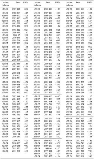
Table A2 Spearman rank correlation values between the independent variables considered in the analysis. Bonferroni correction was applied to the p values and significant correlations (p < 0.05) are starred. DCW – surface water disconnected from the stream network, CCW – continuously connected surface water, MI – Moisture Index, PET – potential evapotranspiration, precip – precipitation, lg – large, ag – agricultural, K_sat – saturated hydraulic conductivity, and n/a – not applicable.

^* Significant correlations (p < 0.05).