the Creative Commons Attribution 3.0 License.
the Creative Commons Attribution 3.0 License.
Multiple causes of nonstationarity in the Weihe annual low-flow series
Bin Xiong
Jie Chen
Chong-Yu Xu
Lingqi Li
Under the background of global climate change and local anthropogenic activities, multiple driving forces have introduced various nonstationary components into low-flow series. This has led to a high demand on low-flow frequency analysis that considers nonstationary conditions for modeling. In this study, through a nonstationary frequency analysis framework with the generalized linear model (GLM) to consider time-varying distribution parameters, the multiple explanatory variables were incorporated to explain the variation in low-flow distribution parameters. These variables are comprised of the three indices of human activities (HAs; i.e., population, POP; irrigation area, IAR; and gross domestic product, GDP) and the eight measuring indices of the climate and catchment conditions (i.e., total precipitation P, mean frequency of precipitation events λ, temperature T, potential evapotranspiration (EP), climate aridity index AIEP, base-flow index (BFI), recession constant K and the recession-related aridity index AIK). This framework was applied to model the annual minimum flow series of both Huaxian and Xianyang gauging stations in the Weihe River, China (also known as the Wei He River). The results from stepwise regression for the optimal explanatory variables show that the variables related to irrigation, recession, temperature and precipitation play an important role in modeling. Specifically, analysis of annual minimum 30-day flow in Huaxian shows that the nonstationary distribution model with any one of all explanatory variables is better than the one without explanatory variables, the nonstationary gamma distribution model with four optimal variables is the best model and AIK is of the highest relative importance among these four variables, followed by IAR, BFI and AIEP. We conclude that the incorporation of multiple indices related to low-flow generation permits tracing various driving forces. The established link in nonstationary analysis will be beneficial to analyze future occurrences of low-flow extremes in similar areas.
- Article
(4392 KB) - Full-text XML
- BibTeX
- EndNote


Low flow is defined as the flow of water in a stream during prolonged dry weather (WMO, 2009). Yu et al. (2014) quantitatively described a low-flow event as a segment of hydrograph during a period of dry weather with discharge values below a preset (relatively small) threshold. According to WMO (2009), annual minimum flows averaged over several days can be used to measure low flows. During low-flow periods, the magnitude of river flow will greatly restrict its various functions (e.g., providing water supply for production and living, diluting waste water, ensuring navigation, meeting ecological water requirement). Therefore, the investigation of the magnitude and frequency of low flows is of primary importance for engineering design and water resources management (Smakhtin, 2001). In recent years, low flows, as an important part of river flow regime, have been attracting an increasing attention of hydrologists and ecologists in the context of the significant impacts of climate change and human activities (HAs; Bradford and Heinonen, 2008; Du et al., 2015; Kam and Sheffield, 2015; Kormos et al., 2016; Liu et al., 2015; Sadri et al., 2016). In general, under the impact of a changing environment, combinations of multiple factors, such as precipitation change, temperature change, irrigation area (IAR) change and construction of reservoirs, can drive various patterns of streamflow changes (Liu et al., 2017; Tang et al., 2016). Unfortunately, when subjected to a variety of influencing forces, low flow is more vulnerable than high flow or mean flow. Therefore, it is a pretty important issue in hydrology to identify low-flow changes, track multiple driving factors and quantify their contributions from the perspective of hydrological frequency analysis.
In hydrological analysis and design, conventional frequency analysis estimates the statistics of a hydrological time series based on recorded data with the stationary hypothesis which means that this series is “free of trends, shifts or periodicity (cyclicity)” (Salas, 1993). However, global warming and human forces have changed climate and catchment conditions in some regions. Time-varying climate and catchment conditions (TCCCs) can affect all aspects of the flow regime, i.e., changing the frequency and magnitude of floods, altering flow seasonality and modifying the characteristics of low flows. The hypothesis of stationarity has been suspected (Milly et al., 2008). If this problematic method is still used, the frequency analysis may lead to high estimation error in hydrological design. Therefore, considerable literature has introduced the concept of hydrologic nonstationarity into analysis of various hydrological variables, such as annual runoff (Arora, 2002; Jiang et al., 2015a; Xiong et al., 2014; Yang and Yang, 2013), flood (Gilroy and Mccuen, 2012; Kwon et al., 2008; Yan et al., 2017; Zhang et al., 2015), low flow (Du et al., 2015; Jiang et al., 2015b; Liu et al., 2015), precipitation (Gu et al., 2017; Mondal and Mujumdar, 2015; Villarini et al., 2010) and so on. Compared with the literature on annual runoff, floods and precipitation, the literature on the nonstationary analysis of low flow is relatively limited.
Previous hydrological literature on frequency analysis of nonstationary hydrological series mainly focuses on two aspects: development of the nonstationary method and exploration of covariates reflecting changing environments. Strupczewski et al. (2001) presented the method of time-varying moment which assumes that the hydrological variable of interest obeys a certain distribution type, but its moments change over time. The method of time-varying moment was modified to be the method of time-varying parameter values for the distribution representative of hydrologic data (Richard et al., 2002). Villarini et al. (2009) presented this method using the generalized additive models for location, scale and shape parameters (GAMLSS; Rigby and Stasinopoulos, 2005), a flexible framework to assess nonstationary time series. The time-varying parameter method can be extended to the physical covariate analysis by replacing time with any other physical covariates (Jiang et al., 2015b; Kwon et al., 2008; López and Francés, 2013; Liu et al., 2015; Villarini and Strong, 2014). For example, Jiang et al. (2015b) used reservoir index as an explanatory variable based on the time-varying copula method for bivariate frequency analysis of nonstationary low-flow series in Hanjiang River, China. Du et al. (2015) took precipitation and air temperature as the explanatory variables to explain the inter-annual variability in low flows of the Weihe River, China (also known as the Wei He River). Liu et al. (2015) took the sea surface temperature in the Nino3 region, the Pacific Decadal Oscillation, the sunspot number (3 years ahead), the winter areal temperature and precipitation as the candidate explanatory variables to explain the inter-annual variability in low flows of Yichang station, China. Kam and Sheffield (2015) ascribed the increasing inter-annual variability of low flows over the eastern United States to the North Atlantic Oscillation and Pacific North America.
To our knowledge, compared with the nonstationary flood frequency analysis, the studies on the nonstationary frequency analysis of low-flow series are not very extensive because of incomplete knowledge of low-flow generation (Smakhtin, 2001). Most of these studies explain nonstationarity of low-flow series only by using climatic indicators or a single indicator of human activity. However, the indicators of catchment conditions (e.g., recession rate) related to physical hydrological processes have seldom been attached in nonstationary modeling of low-flow series. This lack of linking with hydrological processes makes it impossible to accurately quantify the contributions of influencing factors for the nonstationarity of low-flow series, and such a scientific demand for tracing the sources of nonstationarity of low-flow series and qualifying their contributions motivated the present study. The knowledge of low-flow generation has been increased by efforts of hydrologists, which can help develop physical covariates to address nonstationarity. Low flows generally originate from groundwater or other delayed outflows (Smakhtin, 2001; Tallaksen, 1995). Their generation relates to both an extended dry weather period (leading to a climatic water deficit) and complex hydrological processes which determine how these deficits propagate through the vegetation, soil and groundwater system to streamflow (WMO, 2009). Thus, not only climate condition drivers (e.g., potential evaporation exceeds precipitation), but also catchment condition drivers (e.g., the faster hydrologic response rate to precipitation) can cause low flows.
The significant factors such as precipitation, temperature, evapotranspiration (EP), streamflow recession, large-scale teleconnections and human forces may play important roles in influencing low-flow generation (Botter et al., 2013; Giuntoli et al., 2013; Gottschalk et al., 2013; Kormos et al., 2016; Sadri et al., 2016). Gottschalk et al. (2013) presented a derived low-flow probability distribution function with climate and catchment characteristics parameters (i.e., the mean length of dry spells λ−1 and recession constant of streamflow K ) as its distribution parameters. Botter et al. (2013) derived a measurable index ( which can be used for discriminating erratic river flow regimes from persistent river flow regimes. Recently, Van Loon and Laaha (2015) used climate and catchment characteristics (e.g., the duration of dry spells in precipitation and the base-flow index, BFI) to explain the duration and deficit of the hydrological drought event and offered a further understanding of low-flow generation. These studies indicated that climate and catchment conditions play an important role in producing low flows.
The goal of this study is to trace origins of nonstationarity in low flows through developing a nonstationary low-flow frequency analysis framework with the consideration of the time-varying climate and catchment conditions and human activity. In this framework, the climate and catchment conditions are quantified using the eight indices, i.e., meteorological variables (total precipitation P, mean frequency of precipitation events λ, temperature T and potential evapotranspiration), basin storage characteristics (base-flow index, recession constant K) and aridity indexes (climate aridity index AIEP, the recession-related aridity index AIK). The specific objectives of this study are (1) to find the most important index to explain the nonstationarity of low-flow series, (2) to determine the best subset of TCCCs indices and/or human activity indices (i.e., population, POP; irrigation area; and gross domestic product, GDP) for the final model through the stepwise selection method to identify nonstationary mode of low-flow series and (3) to quantify the contribution of selected explanatory variables to the nonstationarity.
This paper is organized as follows. Section 2 describes the methods. The Weihe River basin and available data sets used in this study are described in Sect. 3, followed by a presentation of the results and discussion in Sect. 4. Section 5 summarizes the main conclusions.
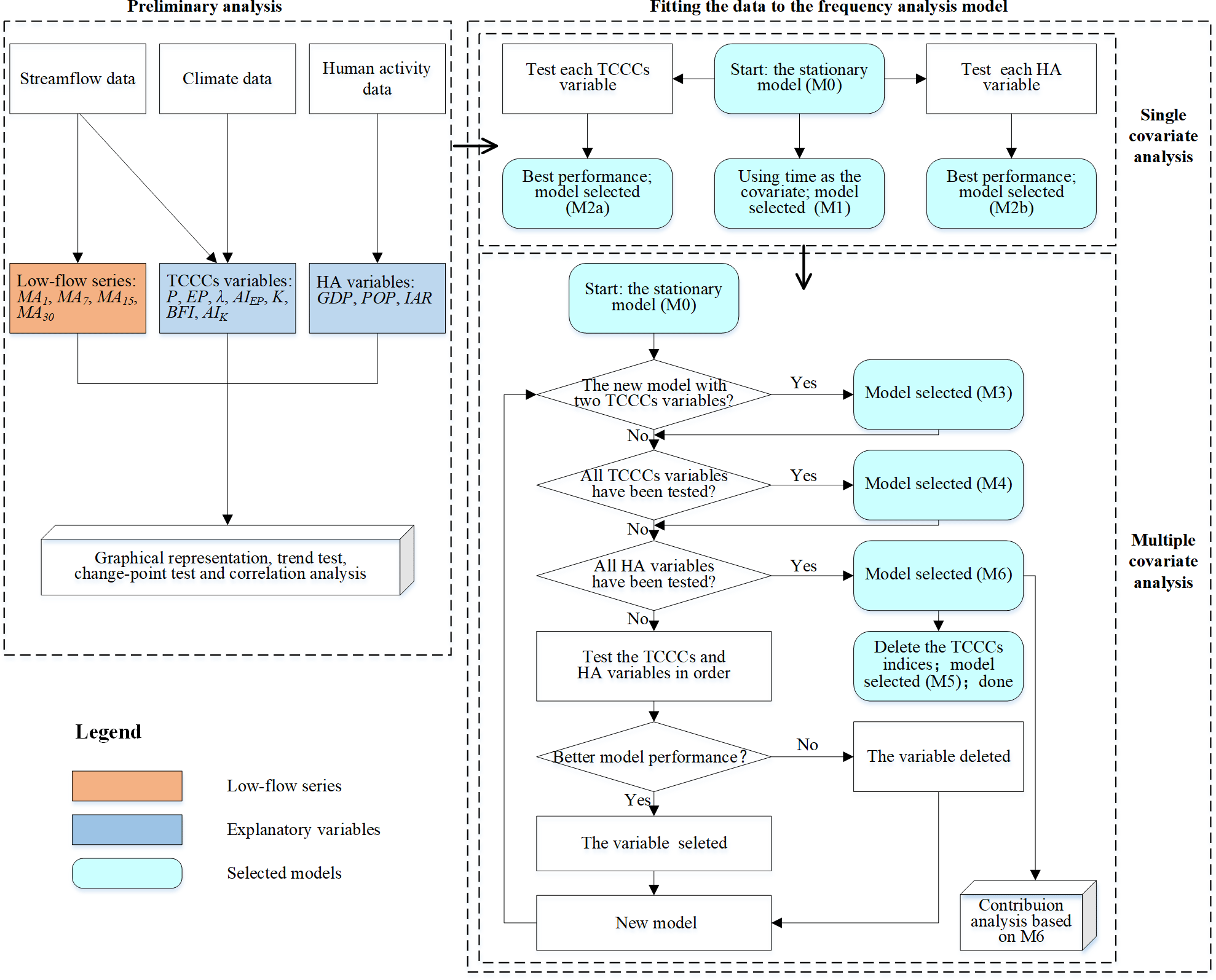
The flowchart of how to organize the nonstationary low-flow frequency analysis framework is shown in Fig. 1. The whole process is divided into three steps. The first step is the preliminary analysis, including the graphical presentation of both explanatory variables and low-flow series, the statistical test for nonstationarity, and the correlations between each explanatory variable and each low-flow series. The second step is the single covariate analysis for the most important explanatory variable. The third step is the multiple covariate analysis for the optimal combination. We use a low-flow frequency analysis model and stepwise regression method to accomplish the last two steps. In the following subsections, first, the low-flow frequency analysis model is constructed based on the nonstationary probability distributions method, in which distribution parameters serving as response variables can vary as functions of explanatory variables. Second, the distribution types used to build the nonstationary model are outlined. Then, the candidate explanatory variables related to the time-varying climate and catchment conditions and human activity are clarified. Finally, estimation of model parameters and selection of models are illustrated.
2.1 Construction of the low-flow nonstationary frequency analysis model
Generally, a nonstationary frequency analysis model can be established based on the time-varying distribution parameters method (Du et al., 2015; López and Francés, 2013; Liu et al., 2015; Richard et al., 2002; Villarini and Strong, 2014). For the nonstationary probability distribution fY(Yt|θt), let Yt be a random variable at time and vector be the time-varying parameters. The number of parameters m in hydrological frequency analysis is generally limited to three or less. The function relationship between the kth parameter and the multiple explanatory variables is expressed as follows:
where are explanatory variables, n is the number of explanatory variables, gk(⋅) is the link function which ensures the compliance with restrictions on the sample space and is usually set to natural logarithm for the given negative predictions and hk(⋅) is the function for nonstationary modeling. The generalized linear model theory (GLM; Dobson and Barnett, 2012) is used to build function relationships between distribution parameters and their explanatory variables. In GLMs, the response relationship can be generally expressed as
where are the GLM parameters.
In order to compare the nonstationary models constructed by various combinations of explanatory variables, Eq. (2) is modified in this study using the dimensionless method for the standard GLM parameters. The value of could be assumed to be equal to its mean ( when all explanatory variables are equal to their mean (, i.e.,
Equation (2) is then modified as
where is the normalized explanatory variable, si is the standard deviation of and are the standard GLM parameters. Letting the link function gk(⋅) be the natural logarithmic function ln (⋅) and be the distribution parameter in with the most significant change, the degree of nonstationarity in low-flow series can be defined as . Then, the contribution of each explanatory variable to could be defined as
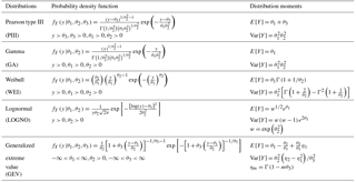
Table 1The probability density functions and moments (the mean and variance) for the candidate distributions in this study.
2.2 Candidate distribution functions
We need to select the form of probability distribution fY(⋅) to determine what type of nonstationary frequency curves will be produced. Various probability distributions have been compared or suggested in modeling of low-flow series (Du et al., 2015; Hewa et al., 2007; Liu et al., 2015; Matalas, 1963; Smakhtin, 2001). An extensive overview of distribution functions for low flow is given in Tallaksen et al. (2004). Following these recommendations, we consider five distributions, i.e., Pearson type III (PIII), gamma (GA), Weibull (WEI), lognormal (LOGNO) and generalized extreme value (GEV) as candidates in this study (Table 1). In the case of Pearson type III distribution, considering that the parameter θ3 of Pearson type III as lower bound should approach zero and the parameter θ3 of GEV is quite sensitive and difficult to be estimated, we assume them to be constant in this study.
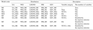
Table 2Description of the developed nonstationary models using time, TCCCs indices and/or HA indices as explanatory variables.
2.3 Candidate explanatory variables
We look for variables that can explain parts of the variations in distribution parameters θt. From the perspective of low-flow generation, the dependency between low-flow regime and both climate and catchment conditions has been presented by previous studies (Botter et al., 2013; Gottschalk et al., 2013; Van Loon and Laaha, 2015). We focus on eight measuring indices: precipitation, mean frequency of precipitation events, temperature, potential evapotranspiration, climate aridity index, base-flow index, recession constant and recession-related aridity index. These indices were chosen to incorporate time-varying climate and catchment conditions in nonstationary modeling of low-flow frequency and serve as candidate explanatory variables. Climate variables (i.e., precipitation, mean frequency of precipitation events, temperature, potential evapotranspiration and climate aridity index) are related to both water supply source and water loss and are therefore selected as candidate variables. It has been shown that the base-flow index and recession constant reflect the storage and release capability of the catchments (Van Loon and Laaha, 2015). The recession-related aridity index reflects both the water supply and storage capability (Botter et al., 2013). In addition to TCCCs indices, the three indices of human activity (irrigation area, population and gross domestic product) are related to water withdrawal loss for agricultural, domestic and industrial purposes and are therefore included. The detailed reasons for selecting all indices are summarized in Table 3. The values of them at each year could be estimated from hydro-meteorological data and human activity data. Annual precipitation (P) and temperature (T) are calculated directly by meteorological data. The remaining TCCCs indices need to be estimated indirectly. Detailed estimation procedures are shown in the following subsections.
2.3.1 Annual mean frequency of precipitation events (λ)
Annual mean frequency of precipitation events is defined as an index to represent the intensity of precipitation recharge to the streamflow:
where Nw(A) is the number of daily rainfall events A (with values more than the threshold 0.5 mm) in wth windows with a length tr; W is the number of windows.
2.3.2 Annual climate aridity index (AIEP)
The ratio of annual potential evaporation to precipitation, commonly known as the climate aridity index, has been used to assess the impacts of climate change on annual runoff (Arora, 2002; Jiang et al., 2015a). The climate aridity index largely reflects the climatic regimes in a region and determines runoff rates (Arora, 2002). Therefore, we choose the annual climate aridity index as a measure of time-varying climate and catchment conditions and estimate its value in a whole region using
where P is annual areal precipitation (mm) and EP is annual areal potential evapotranspiration (mm). The Hargreaves equation (Hargreaves and Samani, 1985) is applied to calculate EP using the R package “Evapotranspiration” (Guo, 2014).
2.3.3 Annual base-flow index (BFI)
The base-flow index (BFI) is defined as the ratio of base flow to total flow. This index has been applied to quantify catchment conditions (e.g., soil, geology and storage-related descriptors) to explain hydrological drought severity (Van Loon and Laaha, 2015). We also choose annual base-flow index as a measure of TCCCs. BFI is estimated using a hydrograph separation procedure in the R package “lfstat” (Koffler and Laaha, 2013).
2.3.4 Annual streamflow recession constant (K)
The recession constant is an important catchment characteristic index measuring the timescale of the hydrological response and reflecting water retention ability in the upstream catchment (Botter et al., 2013). Various estimation methods have been developed to extract recession segments and to parameterize characteristic recession behavior of a catchment (Hall, 1968; Sawaske and Freyberg, 2014; Tallaksen, 1995).
In this study, annual recession analysis (ARA) is performed to obtain the annual streamflow recession constant (K). In ARA, the linearized Dupuit–Boussinesq equation is used to parameterize characteristic recession behavior of a catchment and is written as
where Qt is the value at time t. Equation (8) is investigated by plotting data points against Qt of all extracted recession segments from hydrographs at each year. The criteria of recession segment extraction are based on the Manual on Low-flow Estimation and Prediction (WMO, 2009). Then, the annual recession rate (K−1) is estimated as the slope of the fitted straight line of these data points with the least-squares method. We calculated K using the R package “lfstat” (Koffler and Laaha, 2013).
2.3.5 Annual recession-related aridity index (AIK)
In this study, the recession-related aridity index is defined as the ratio of recession rate (K−1) to mean precipitation frequency (λ), denoted as
This ratio plays an important role in controlling the river flow regime (Botter et al., 2013; Gottschalk et al., 2013) and serves as an indicator measuring the recession-related aridity degree of the streamflow in the river channel. For example, the faster recession process or lower precipitation frequency may lead to increased runoff loss or decreased precipitation supply. Consequently, the higher the value AIK is, the more likely low-flow events occur, and vice versa.
2.4 Parameter estimation
The model parameters including and need to be estimated. are estimated from outputs of stationary frequency analysis through the maximum likelihood method. We have
where yt is observed low flow at time t and N is the number of samples. The parameters are estimated through the maximum likelihood method to produce nonstationary low-flow frequency curves:
The residuals (normalized randomized quintile residuals) are used to test the goodness of fit of fitted model objects (Dunn and Symth, 1996):
where FY(⋅) is the cumulative distribution of yt and is the inverse function of the standard normal distribution. The distribution of the true residuals converges to standard normal if the fitted model is correct. A worm plot (Buuren and Fredriks, 2001) is used to check whether have a standard normal distribution.
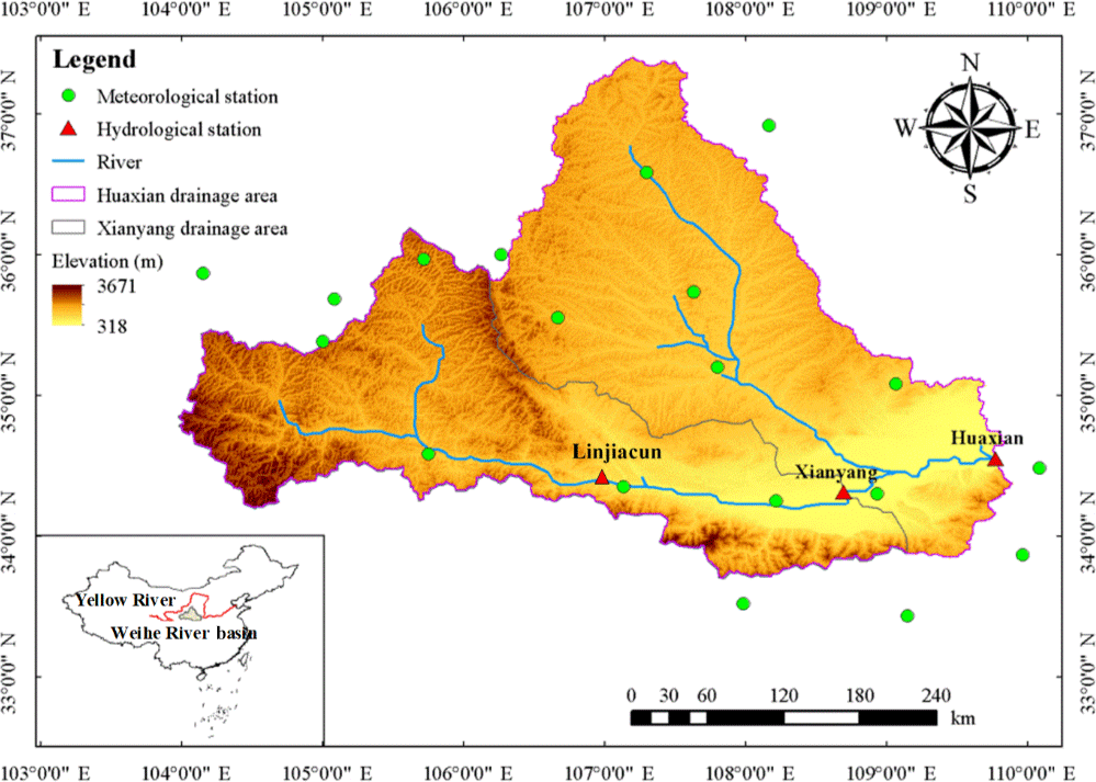
Figure 2Location, topography, hydro-meteorological stations and river systems of the Weihe River basin.
Table 3The summary of candidate explanatory variables and reason of selection.
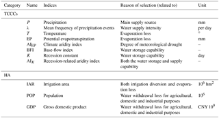

Figure 3The annual minimum low flows and fitted trend lines in both Huaxian (H) and Xianyang (X) gauging stations.
2.5 Model selection
Model selection contains the selection of the type of probability distribution and the selection of the explanatory variables to explain the response variables (i.e., distribution parameters θ1 and θ2). In order to obtain the final optimal model, the selection of the explanatory variables for θ1 and θ2 is conducted by stepwise selection strategies (Stasinopoulos and Rigby, 2007; Venables, 2002): i.e., select a best subset of candidate explanatory variables for θ1 using a forward approach (which starts with no explanatory variable in the model and tests the addition of each explanatory variable using a chosen model fit criterion); given this subset for θ1 select another subset for θ2 (forward). The stepwise selection strategies can get a series of stepwise models with different numbers of explanatory variables, as shown in Fig. 1. In order to detect how the number of explanatory variables influences the performance of the model for describing nonstationarity, we investigate the eight types of stepwise models as shown in Table 2: the zero-covariate model or stationary model (M0), the time covariate model (M1), the single physical covariate model M2 (single TCCCs covariate model M2a or single HA covariate model M2b), two TCCCs covariates model (M3), the optimal TCCCs covariates model (M4), the optimal HA covariates model (M5) and the final model (M6). The model fit criterion is based on the Akaike's information criterion (AIC; Akaike, 1974) as shown by the following
where ML is the log-likelihood in Eq. (11) and df is the number of degrees of freedom. The model with the lower AIC value was considered better.
3.1 The study area
The Weihe River, located in the southeast of the northwest Loess Plateau, is the largest tributary of the Yellow River, China. The Weihe River has a drainage area of 134 766 km2, covering the coordinates of – N, – E (Fig. 2). This catchment generally has a semi-arid climate, with extensive continental monsoonal influence. Average annual precipitation of the whole area over the period 1954–2009 is about 540 mm and has a wide range (400–1000 mm) in various regions. Under the significant impacts of climate change and human activities in the Weihe River basin in recent decades, the hydrological regime of the river has changed over time (Du et al., 2015; Jiang et al., 2015a; Xiong et al., 2015).
In the Weihe basin, the impacts of agricultural irrigation on runoff have been found to be significant (Jiang et al., 2015a; Lin et al., 2012). Lin et al. (2012) mentioned that the annual runoff of the Weihe River was significantly affected by irrigation diversion of the Baoji Gorge irrigation district. The irrigated area of the Baoji Gorge irrigation district increased over time since the founding of P.R. China in 1949, and, due to one influential irrigation system project in that area, it became more than twice as large as the original irrigation area since 1971. Jiang et al. (2015a) demonstrated that, in the Weihe basin, irrigated area, as compared with the other indices, e.g., population, gross domestic product and cultivated land area, was a more suitable human explanatory variable for explaining the time-varying behavior of annual runoff. With the above background, it is important to consider the effects of human activities that mainly originate from irrigation diversion, especially for studying low-flow series in this basin. The estimations of annual recession rate (K−1) by the daily streamflow data are expected to incorporate the information of impacts of water diversions on the low flows in the river channel.
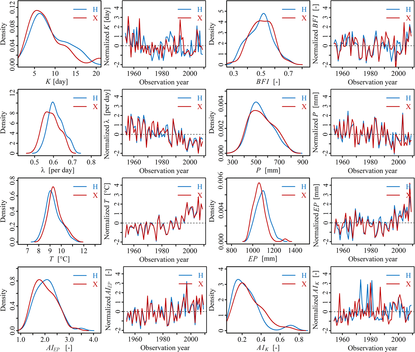
Figure 4Frequency distributions (using the kernel density estimations) and time series processes of TCCCs variables in both Huaxian (H) and Xianyang (X) stations.
3.2 Data
We used daily streamflow records (1954–2009) provided by the Hydrology Bureau of the Yellow River Conservancy Commission from both Huaxian station (with a drainage area of 106 500 km2) and Xianyang station (with a drainage area of 46 480 km2). Low-flow extreme events were selected from the daily streamflow series using the widely used annual minimum series method (WMO, 2009). AMn is the annual minimum n-day flow during hydrological year beginning on 1 March. Consequently, AM1, AM7, AM15 and AM30 are selected as low-flow extreme events in this study. The original measure unit of streamflow data (m3 s−1) is converted to 10−4 m3 s−1 km−2 for convenience of comparison of results between the Huaxian and Xianyang gauging stations
We downloaded daily total precipitation and daily mean air temperature records for 19 meteorological stations over the basin from the National Climate Center of the China Meteorological Administration (source: http://www.cma.gov.cn/). The areal average daily series of both variables above Huaxian and Xianyang stations are calculated using the Thiessen polygon method (Szolgayova et al., 2014; Thiessen, 1911). The annual average temperature (T) and annual total precipitation (P) over the period 1954–2009 are calculated for each catchment.
Human activity data (i.e., gross domestic product, population and irrigation area) were taken from annals of statistics provided by the Shaanxi Provincial Bureau of Statistics (http://www.shaanxitj.gov.cn/) and Gansu Provincial Bureau of Statistics (source: http://www.gstj.gov.cn/).
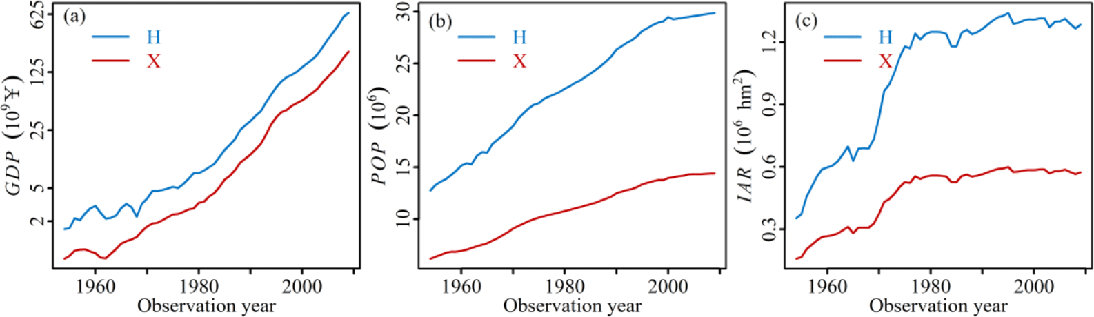
Figure 5HA indices in both Huaxian (H) and Xianyang (X). (a), (b) and (c) are for gross domestic production (GDP), population (POP) and irrigated area (IAR), respectively.
4.1 Identification of nonstationarity
The graphical representation and statistical test provide a preliminary analysis for low-flow nonstationarity. The graphical representations of time-series data help visualize the trends of related variables (i.e., low flow, TCCCs and HA variables), the density distributions of TCCCs variables, and the correlations between low-flow variables and these explanatory variables. In Fig. 3, four annual minimum streamflow series (AM1, AM7, AM15 and AM30) in both Huaxian and Xianyang gauging stations show overall decreasing trends, as indicated by the fitted (dashed) trend lines. Compared with Huaxian, Xianyang has a larger runoff modulus (the flow per square kilometer) and a larger decrease in annual minimum streamflow series. For example, the decline slope of AM30 is −0.0725 (10−4 m3 s−1 km−2 yr−1) in Huaxian station while Xianyang station it is −0.1338 (10−4 m3 s−1 km−2 yr−1).
Figure 4 shows the kernel density estimations and time processes of TCCCs variables for both Huaxian (H) and Xianyang (X) stations. The results show that these variables have different variation patterns. For example, the mean frequency of precipitation events (λ) has a decreasing trend, while temperature (T) has an increasing trend. As presented by Fig. 5, three HA variables have a significant upward trend, especially the irrigation area which is increased greatly after about 1970, suggesting that the impact of human activities in this basin has increased over time.
Table 4The results of trend test and change-point detection for both the four low-flow series and TCCCs variables in Huaxian and Xianyang.
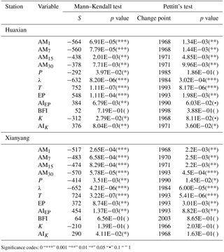
Significance codes: 0 “***” 0.001 “**” 0.01 “*” 0.05 “•” 0.1 “ ” 1
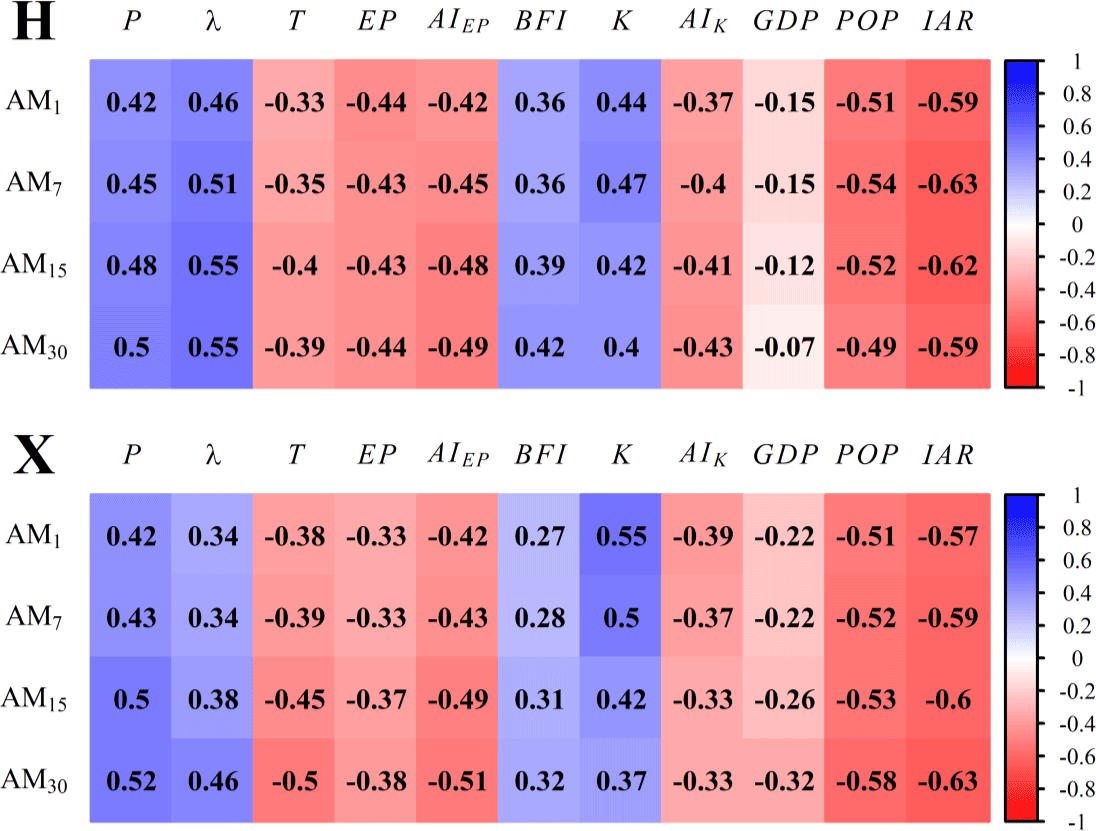
Figure 6The Pearson correlation coefficients matrix between the annual minimum flow series and candidate explanatory variables in Huaxian (H) and Xianyang (X) stations; the darker color intensity represents a higher level of correlation (blue indicates positive correlation and red indicates negative correlations).
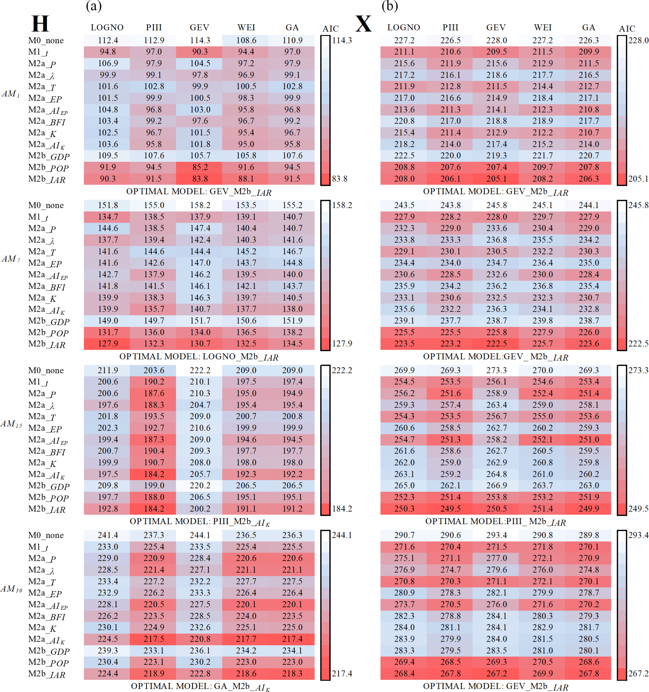
Figure 7Comparisons among M0, M1 and M2 based on the AIC values for the four observed low-flow series in Huaxian (H) at (a) and Xianyang (X) at (b); darker red color represents a higher goodness of fit.
The significance of trends in the four annual minimum streamflow series and TCCCs variables is tested by the Mann–Kendall trend test (Kendall, 1975; Mann, 1945; Yue et al., 2002), and the change points in these series are detected by Pettitt's test (Pettitt, 1979). The results in Table 4 show that, in both Huaxian and Xianyang stations, the decreasing trends in all the four low-flow series (AM1, AM7, AM15 and AM30) and two explanatory variables (λ and P), as well as the increasing trends in T, EP, and AIEP are significant at the 0.05 level (Table 4), but BFI shows no significant trends. However, K and AIK had significantly decreasing trends only in Huaxian station (p value <0.05). The results of change-point detection show that all low-flow series are located at 1968–1971 (p value <0.05) except AM30 at Xianyang station whose change point is located at 1993 (p value <0.05); for the eight candidate explanatory variables, the change points of the variables related to temperature (T, EP, AIEP) in both stations are located at 1990–1993 (p value <0.05), the change points of the variables related to precipitation (λ, P) in both stations are close at 1984–1990 (p value ≤0.186) and the change points of the variables related to streamflow recession (K, AIK) in Huaxian station are located at 1968–1971 (p value <0.05). However, BFI in both stations and K and AIK in Xianyang station show no significant change points.
A preliminary attribution analysis is performed using the Pearson correlation matrix to investigate the relations between the annual minimum series and eight candidate explanatory variables. Figure 6 indicates that there are significant linear correlations between the four minimum low-flow series (AM1, AM7, AM15 and AM30) and all the explanatory variables except GDP have the absolute values of Pearson correlation coefficients larger than 0.27 (p value <0.05). These potential physical causes of nonstationarity in low flows are further considered by establishing the low-flow nonstationary model with TCCCs and HA variables in the following section.
4.2 Nonstationary frequency analysis models
4.2.1 Single covariate models
Figure 7 presents the AIC values of the four types of models (M0, M1, M2a and M2b) fitted for the low-flow series (AM1, AM7, AM15 and AM30). Some interesting results are shown as follows. First, nonstationary models (M1, M2a and M2b) have lower AIC values than stationary model (M0), which suggests that nonstationary models are worth considering. Second, for Huaxian station, irrespective of the chosen explanatory variables, the distribution type plays an important role in modeling nonstationary low-flow series. For example, PIII, GA and WEI distributions in AM15 and AM30 cases have lower AIC values than LOGNO and GEV distributions. However, for Xianyang, choosing a suitable explanatory variable may be more important than choosing a distribution type. For example, variables t, P, T, AIEP, POP and IAR in most cases have lower AIC values than the other explanatory variables. Finally, in Huaxian, the lowest AIC values for modeling AM1, AM7, AM15 and AM30 are found in GEV_M2b_IAR, LOGNO_M2b_IAR, PIII_M2a_AIK and GA_M2a_AIK, respectively, while in Xianyang the lowest AIC values for modeling AM1, AM7, AM15 and AM30 are found in GEV_M2b_IAR, GEV_M2b_IAR, PIII_M2b_IAR and GEV_M2b_IAR, respectively. These results indicated that for explaining nonstationarity of low flow in Huaxian station, IAR is the most dominant HA variable and AIK is the most dominant TCCCs variable, while in Xianyang the most dominant HA variable is IAR and the most dominant TCCCs variables causing nonstationarity in AM1, AM7, AM15 and AM30 are K, AIEP, AIEP and T, respectively.
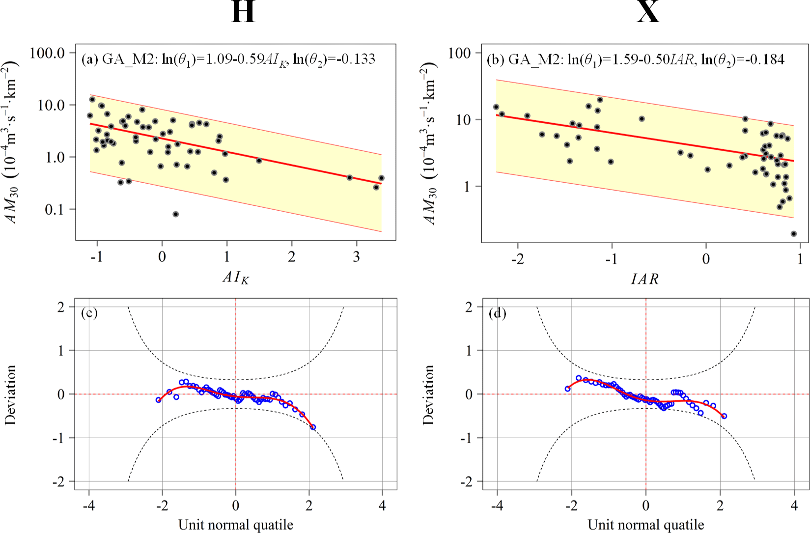
Figure 8Performance assessments of GA_M2 for AM30 in Huaxian (H) on the left panel and Xianyang (X) on the right panel. (a) and (b) are the centile curves plots of GA_M2 (red lines represent the centile curves estimated by GA_M2; the 50th centile curves are indicated by thick red; the yellow-filled areas are between the 5th and 95th centile curves; the black points indicate the observed series); (c) and (d) are the worm plots of GA_M2 for the goodness-of-fit test; a reasonable model fit should have the data points fall within the 95 % confidence intervals (between the two red dashed curves).
Figure 8 shows the diagnostic assessment of the GA_M2 model (with the optimal explanatory variable) for AM30 in both Huaxian and Xianyang stations. The centile curve plots of GA_M2 (Fig. 8a and b) show the observed values of AM30, the estimated median and the areas between the 5th and 95th centile. Figure 8a shows the response relationship between AM30 and AIK in Huaxian: the increase in AIK means the smaller magnitude of low-flow events because a high value of AIK (faster stream recession or fewer rainy days) may lead to faster water loss or less supply. In Fig. 8b, the higher values of IAR means the smaller magnitude of low-flow events, which suggests that IAR plays an important role in driving low-flow generation in Xianyang. Figure 8c and d show that the worm points are within the 95 % confidence intervals, thereby indicating a good model fit and a reasonable model construction.

Figure 9Comparisons of performance of stationary model (M0), time covariate model (M1) and physical covariate models (M2a, M2b, M3, M4, M5 and M6 with their corresponding optimal explanatory variables) for AM30 in Huaxian (H) at (a) and Xianyang (X) at (b).
4.2.2 Multiple covariate models
Figure 9 shows the AIC values of the stationary model (M0), time covariate model (M1) and physical covariate models (M2a, M2b, M3, M4, M5 and M6) for AM30. As shown in Fig. 9, M4 (nonstationary GA distribution with the optimal TCCCs variables) has a good performance; after adding the HA variables, M6 with the lowest AIC value is attained; it can be found that the combination of multiple TCCCs variables plays a major role in changing the low flows of the Weihe River, but the influence of HA variables should not be ignored.
Table 5The summary of frequency analysis using GA distribution for AM30 in Huaxian and Xianyang.
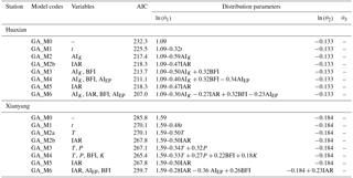
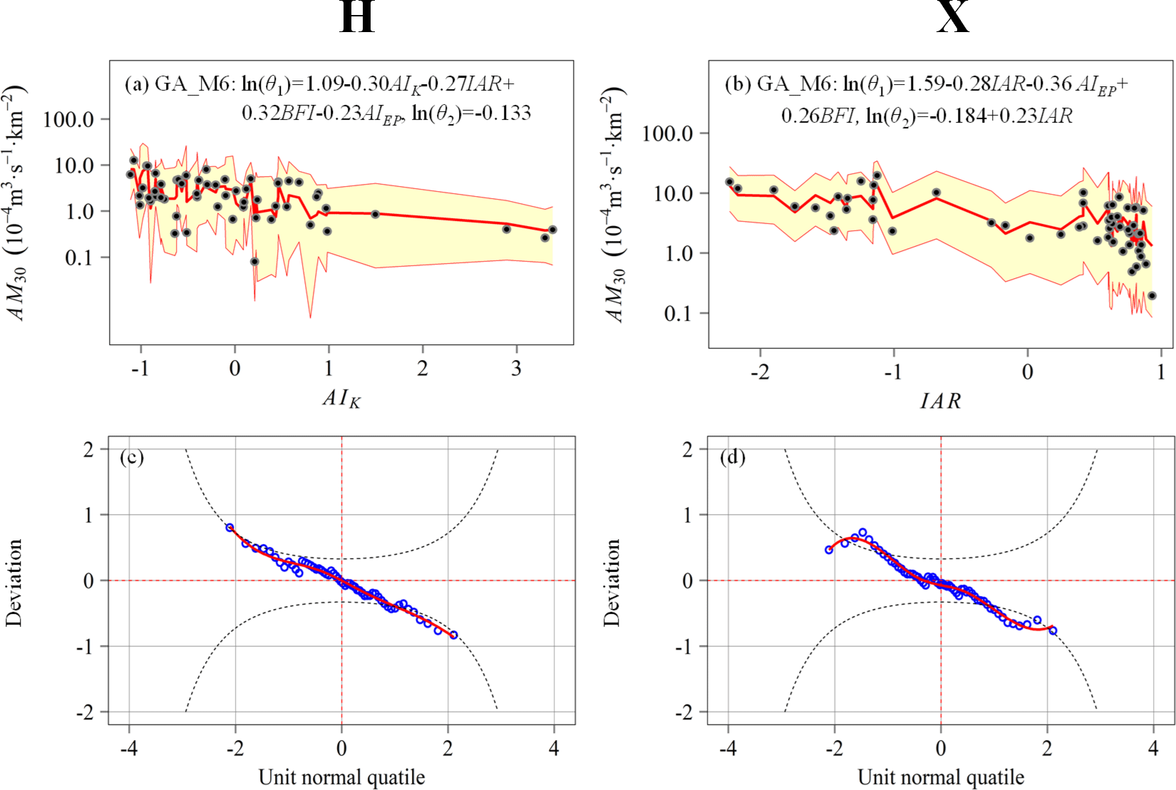
Figure 10Performance assessments of GA_M6 for AM30 in Huaxian (H) on the left panel and Xianyang (X) on the right panel. (a) and (b) are the centile curves plots of GA_M6 (red lines represent the centile curves estimated by GA_M6; the 50th centile curves are indicated by thick red; the yellow-filled areas are between the 5th and 95th centile curves; the filled black points indicate the observed series); (c) and (d) are the worm plots of GA_M6 for the goodness-of-fit test; a reasonable model fit should have the data points fall within the 95 % confidence intervals (between the two red dashed curves).
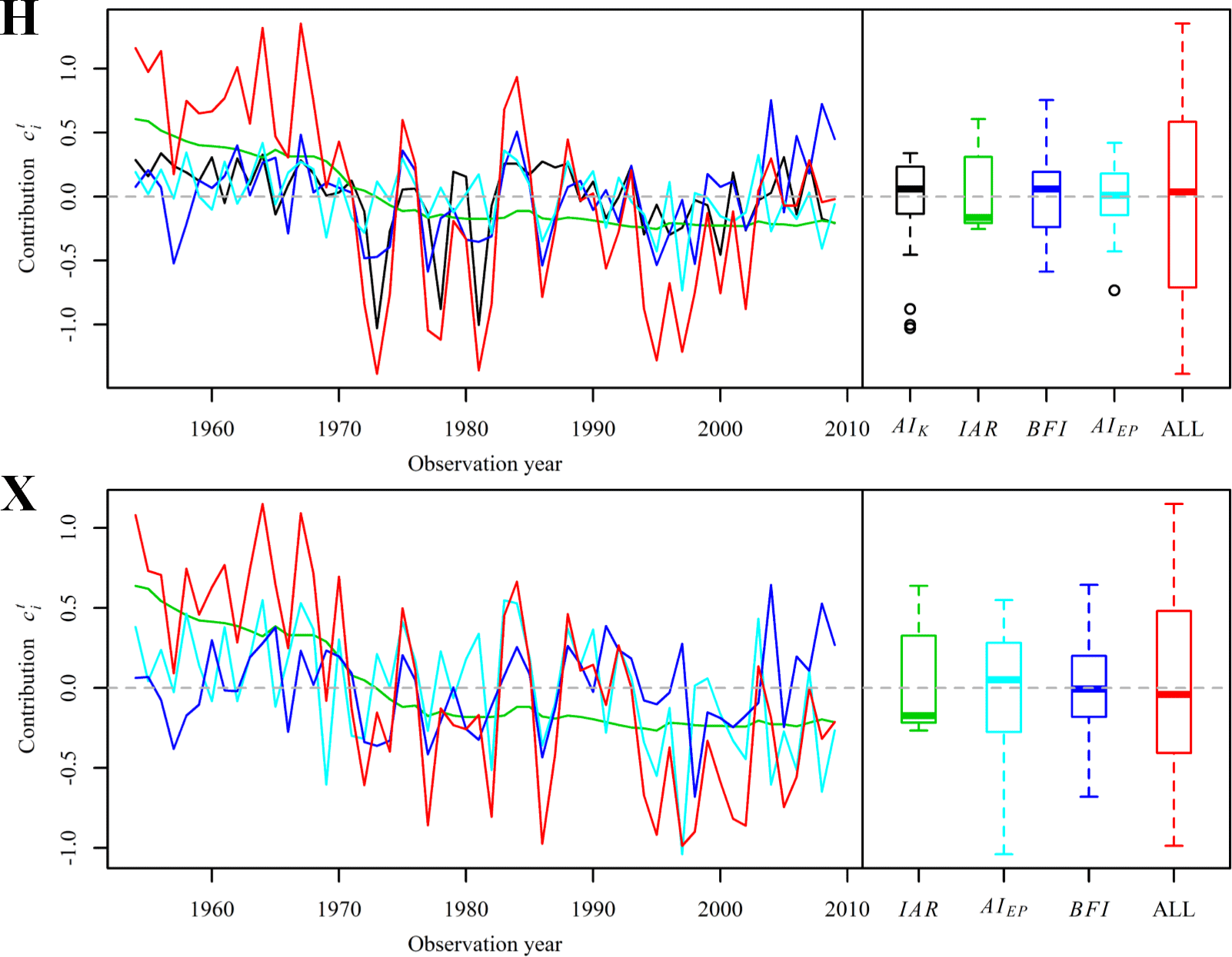
Figure 11Contribution of selected explanatory variables to in different periods based on GA_M6.
A summary of frequency analysis based on nonstationary GA distribution AM30 is presented in Table 5. We choose to focus on M4, M5 and M6. When only using TCCCs variables to model nonstationary low-flow frequency distribution, the results of M4 show the optimal combination of explanatory variables for all low-flow series contains more than three variables. For example, for AM30 of Huaxian, the optimal combination of TCCCs variables includes AIK, BFI and AIEP. When only HA variables are used, the results of M5 show IAR is important to the low flows in this area. And M4 has a better performance than M5. When using both TCCCs variables and HA variables, the results of M6 show the optimal combination contains multiple TCCCs variables and the irrigation area. For Huaxian, the optimal combination of all explanatory variables is AIK, IAR, BFI and AIEP, while for Xianyang, the optimal combination is IAR, AIEP and BFI. We can also find that if two TCCCs variables are highly correlated, they do not seem to be selected as the explanatory variables at the same time. For example, in terms of air temperature (T), evapotranspiration and the climate aridity index (AIEP), only one of them will appear in the optimal combination. This suggests that multicollinearity problem in the multiple variables analysis can be reduced, which will help obtain more reliable GLM parameters for contribution analysis.
The diagnostic assessment of the GA_M6 model for AM30 at two stations is presented by Fig. 10. The centile curve plots of GA_M6 (Fig. 10a and b) show a more sophisticated nonstationary modeling than GA_M2 (Fig. 8). When using GA_M6 to model AM30 in Huaxian (Fig. 10a), similar to GA_M2, the lower low flows are found to also correspond to a higher value of AIK, but GA_M6 is able to identify the more complex variation patterns of low flows through the incorporation of IAR, BFI and AIEP. Figure 10c and d show that the data points of worm plots of GA_M6 are almost within the 95 % confidence intervals, thereby indicating an acceptable model fit and a reasonable model construction.
Figure 11 presents the contribution of each selected explanatory variable to in the observation year based on GA_M6 for AM30 in Huaxian and Xianyang. We can find that for Huaxian, the simulation value of frequently occurs below during the two periods of about 1970–1982 and 1993–2003, which is in accordance with the observed decrease in AM30 of Huaxian station during these periods. In the former period 1970–1982, both AIK and BFI contribute a lot of negative amount to , whereas, during 1993–2003, the contribution of both AIK and BFI decreases significantly. However, IAR has almost equal negative contribution to in both periods. Unlike the former three variables, the significant negative contribution of AIEP is only found in 1993–2003. For AM30 of Xianyang, the contribution of IAR, AIEP and BFI is similar to that at Huaxian station in two periods; however, AIK is not included in the final model.
4.3 Discussion
The impacts of both human activities and climate change on low flows of the study area led to time-varying climate and catchment conditions. Nonstationary modeling for annual low-flow series using TCCCs variables and/or HA variables as explanatory variables is clearly different from either the stationary model (M0) or the time covariate model (M1). The result demonstrates that considering multiple drivers (e.g., the variability in catchment conditions), especially in such an artificially influenced river, is necessary for nonstationary modeling of annual low-flow series.
In this study area, nonstationary modeling considering TCCCs is supported by the following facts and findings. For human activities, an important milestone representative is the completion and operation of the irrigation system on the plateau in the Baoji Gorge irrigation district since 1971 (Sect. 3.1). Figure 5c shows the change in irrigation area in this basin. And the change-point detection test in Sect. 4.1 shows that significant change points of low-flow series occur exactly at around 1971. This result demonstrates that changes in AM30 may involve a consequence of this project. In addition to human activities, climate change also makes a considerable contribution to nonstationarity of low flows, as suggested by nonstationary modeling using TCCCs variables with stepwise analysis. Actually, climate driving pattern may strengthen after nearly 1990, which is indicated by change-point detection test of both annual mean temperature (T) and annual precipitation (P) as well as the behavior of annual low-flow series after nearly 1990. There are two faster recession periods, the 1970s and the 1990s, as shown in Fig. 4. The reasons for the faster recession are likely to be related to the above-mentioned project (e.g., the increasing diversion for irrigation) and climate change (e.g., the intensified evaporation) but also could be human alterations on catchment properties, such as vegetation cover change. In conclusion, the temporal variability in irrigation area, air temperature, precipitation (the frequency and volume of rain events) and streamflow recession should be the main driving factors of generating low-flow regimes in this basin. Overall, the causes of nonstationarity in the category for two gauging stations have no clear difference but have some differences in the relative importance. As shown in Table 5, when modeling the low-flow series of Huaxian using TCCCs variables, the optimal model (M4) preferred the variables that are related to recession process; however, for Xianyang, the preferred variables are related to temperature. The reason for this may be that, as a downstream station, Huaxian station suffers more intensive human activity, so that the importance of temperature change to the low-flow change is reduced meanwhile the importance of streamflow recession (related to the capability of water storage) change is enhanced. Ignoring the negative impacts of the errors in estimating annual recession constants (K) which are caused by insufficient data points of extracted stream segments at some wet years may lead to the propagation of high errors in annual recession analysis and accordingly affect the quality of nonstationary frequency analysis when K is used as an explanatory variable. Further study will give a more reliable estimation of K through the improvement of annual recession analysis. In addition, it should be noted that the population recorded in the annals of statistics may not be equal to the actual population living in the catchment. If the population in the annals is used as the explanatory variable, this difference may lead to the uncertainty of model parameter estimations. Nonetheless, it is the best population data so far and the explanatory variable POP is excluded in the final model (M6).
There is an increasing need to develop an effective nonstationary low-flow frequency model to deal with nonstationarities caused by climate change and time-varying anthropogenic activities. In this study, time-varying climate and catchment conditions in the Weihe River basin were measured by annual time series of the eight indices, i.e., total precipitation (P), mean frequency of precipitation events (λ), temperature (T), potential evapotranspiration, climate aridity index (AIEP), base-flow index, recession constant (K) and the recession-related aridity index (AIK). The nonstationary distribution model was developed using these eight TCCCs indices and/or three HA indices as candidate explanatory variables for frequency analysis of time-varying annual low-flow series caused by multiple drivers. The main driving forces of the decrease in low flows in the Weihe River include reduced precipitation, warming climate, increasing irrigation area and faster streamflow recession. Therefore, a complex deterioration mechanism resulting from these factors demonstrates that, in this arid and semi-arid area, the water resources could be vulnerable to adverse environmental changes, thus portending increasing water shortages. The nonstationary low-flow model considering TCCCs can provide the knowledge of low-flow generation mechanism and give a more reliable design of low flows for infrastructure and water supply.
The data used in this paper can be requested by contacting the corresponding author Lihua Xiong at xionglh@whu.edu.cn.
The authors declare that they have no conflict of interest.
The study was financially supported by the National Natural Science
Foundation of China (NSFC grants 51525902 and 51479139) and projects from
State Key Laboratory of Water Resources and Hydropower Engineering Science,
Wuhan University. We greatly appreciate the editor and three reviewers for
their insightful comments and constructive suggestions that helped us to
improve the manuscript.
Edited by:
Fuqiang Tian
Reviewed by: Xiaohong Chen, Dengfeng Liu,
and one anonymous referee
Akaike, H.: A new look at the statistical model identification, IEEE T. Automat. Contr., 19, 716–723, 1974.
Arora, V. K.: The use of the aridity index to assess climate change effect on annual runoff, J. Hydrol., 265, 164–177, 2002.
Botter, G., Basso, S., Rodriguez-Iturbe, I., and Rinaldo, A.: Resilience of river flow regimes, P. Natl. Acad. Sci. USA, 110, 12925–12930, 2013.
Bradford, M. J. and Heinonen, J. S.: Low Flows, Instream Flow Needs and Fish Ecology in Small Streams, Can. Water Resour. J., 33, 165–180, 2008.
Buuren, S. V. and Fredriks, M.: Worm plot: a simple diagnostic device for modelling growth reference curves, Stat. Med., 20, 1259–1277, 2001.
Dobson, A. J. and Barnett, A. G.: An Introduction to Generalized Linear Models, Third Edition, J. R. Stat. Soc., 11, 272–272, 2012.
Du, T., Xiong, L., Xu, C.-Y., Gippel, C. J., Guo, S., and Liu, P.: Return period and risk analysis of nonstationary low-flow series under climate change, J. Hydrol., 527, 234–250, 2015.
Dunn, P. K. and Symth, G. K.: Randomized quantile residuals, J. Comput. Graph. Stat., 5, 236–244, 1996.
Gilroy, K. L. and Mccuen, R. H.: A nonstationary flood frequency analysis method to adjust for future climate change and urbanization, J. Hydrol., 414–415, 40–48, 2012.
Giuntoli, I., Renard, B., Vidal, J. P., and Bard, A.: Low flows in France and their relationship to large-scale climate indices, J. Hydrol., 482, 105–118, 2013.
Gottschalk, L., Yu, K.-X., Leblois, E., and Xiong, L.: Statistics of low flow: Theoretical derivation of the distribution of minimum streamflow series, J. Hydrol., 481, 204–219, 2013.
Gu, X., Zhang, Q., Singh, V. P., and Shi, P.: Changes in magnitude and frequency of heavy precipitation across China and its potential links to summer temperature, J. Hydrol., 547, 718–731, 2017.
Guo, D.: An R Package for Implementing Multiple Evapotranspiration Formulations, International Environmental Modelling and Software Society, in: Proceedings of the 7th International Congress on Environmental Modelling and Software, edited by: Ames, D. P., Quinn, N. W. T., Rizzoli, A. E., 15–19 June, San Diego, California, USA, ISBN-13: 978-88-9035-744-2, 2014.
Hall, F. R.: Base flow recessions: A review, Water Resour. Res., 4, 973–983, 1968.
Hargreaves, G. H. and Samani, Z. A.: Reference Crop Evapotranspiration From Temperature, Appl. Eng. Agric, 1, 96–99 1985.
Hewa, G. A., Wang, Q. J., McMahon, T. A., Nathan, R. J., and Peel, M. C.: Generalized extreme value distribution fitted by LH moments for low-flow frequency analysis, Water Resour. Res., 43, 227–228, 2007.
Jiang, C., Xiong, L., Wang, D., Liu, P., Guo, S., and Xu, C.-Y.: Separating the impacts of climate change and human activities on runoff using the Budyko-type equations with time-varying parameters, J. Hydrol., 522, 326–338, 2015a.
Jiang, C., Xiong, L., Xu, C.-Y., and Guo, S.: Bivariate frequency analysis of nonstationary low – series based on the time – copula, Hydrol. Process., 29, 1521–1534, 2015b.
Kam, J. and Sheffield, J.: Changes in the low flow regime over the eastern United States (1962–2011): variability, trends, and attributions, Climatic Change, 135, 639–653, 2015.
Kendall, M. G.: Rank Correlation Methods, Griffin, London, 1975.
Koffler, D. and Laaha, G.: LFSTAT – Low-Flow Analysis in R, Egu General Assembly, Vienna, Austria, 15, available at: https://cran.r-project.org/web/packages/lfstat/index.html (last access: 15 March 2017), 2013.
Kormos, P. R., Luce, C. H., Wenger, S. J., and Berghuijs, W. R.: Trends and sensitivities of low streamflow extremes to discharge timing and magnitude in Pacific Northwest mountain streams, Water Resour. Res., 52, 4990–5007, 2016.
Kwon, H.-H., Brown, C., and Lall, U.: Climate informed flood frequency analysis and prediction in Montana using hierarchical Bayesian modeling, Geophys. Res. Lett., 35, L05404, https://doi.org/10.1029/2007GL032220, 2008.
López, J. and Francés, F.: Non-stationary flood frequency analysis in continental Spanish rivers, using climate and reservoir indices as external covariates, Hydrol. Earth Syst. Sci., 17, 3189–3203, https://doi.org/10.5194/hess-17-3189-2013, 2013.
Lin, Q. C., Huai-En, L. I., and Xi-Jun, W. U.: Impact of Water Diversion of Baojixia Irrigation Area to the Weihe River Runoff, Yellow River, 34, 106–108, 2012.
Liu, D., Guo, S., Lian, Y., Xiong, L., and Chen, X.: Climate-informed low-flow frequency analysis using nonstationary modelling, Hydrol. Process., 29, 2112–2124, 2015.
Liu, J., Zhang, Q., Singh, V. P., and Shi, P.: Contribution of multiple climatic variables and human activities to streamflow changes across China, J. Hydrol., 545, 145–162 2017.
Mann, H. B.: Nonparametric Tests Against Trend, Econometrica, 13, 245–259, 1945.
Matalas, N. C.: Probability distribution of low flows, U.S. Geological Survey professional Paper, 434-A, 1963.
Milly, P. C. D., Betancourt, J., Falkenmark, M., Hirsch, R. M., Kundzewicz, Z. W., Lettenmaier, D. P., and Stouffer, R. J.: Stationarity Is Dead: Whither Water Management?, Science, 319, 573–574, 2008.
Mondal, A. and Mujumdar, P. P.: Modeling non-stationarity in intensity, duration and frequency of extreme rainfall over India, J. Hydrol., 521, 217–231, 2015.
Pettitt, A. N.: A Non-Parametric Approach to the Change-Point Problem, J. R. Stat. Soc., 28, 126–135, 1979.
Richard, W. K., Marc, B. P., and Philippe, N.: Statistics of extremes in hydrology, Adv. Water Resour., 25, 1287–1304, 2002.
Rigby, R. A. and Stasinopoulos, D. M.: Generalized additive models for location, scale and shape, Appl. Statist., 54, 507–554, 2005.
Sadri, S., Kam, J., and Sheffield, J.: Nonstationarity of low flows and their timing in the eastern United States, Hydrol. Earth Syst. Sci., 20, 633–649, https://doi.org/10.5194/hess-20-633-2016, 2016.
Salas, J. D.: Analysis and modeling of hydrologic time series, Handbook of Hydrology, McGraw Hill, NewYork, Chapter 19, 1–72, 1993.
Sawaske, S. R. and Freyberg, D. L.: An analysis of trends in baseflow recession and low-flows in rain-dominated coastal streams of the pacific coast, J. Hydrol., 519, 599–610, 2014.
Smakhtin, V. U.: Low flow hydrology – a review, J. Hydrol., 240, 147–186, 2001.
Stasinopoulos, D. M. and Rigby, R. A.: Generalized additive models for location scale and shape (GAMLSS) in R, J. Stat. Softw., 23, https://doi.org/10.18637/jss.v023.i07, 2007.
Strupczewski, W. G., Singh, V. P., and Feluch, W.: Non-stationary approach to at-site flood frequency modeling I. Maximum likelihood estimation, J. Hydrol., 248, 123–142, 2001.
Szolgayova, E., Parajka, J., Blöschl, G., and Bucher, C.: Long term variability of the Danube River flow and its relation to precipitation and air temperature, J. Hydrol., 519, 871–880, 2014.
Tallaksen, L. M.: A review of baseflow recession analysis, J. Hydrol., 165, 349–370, 1995.
Tallaksen, L. M., Madsen, H., and Hisdal, H.: Hydrological Drought- Processes and Estimation Methods for Streamflow and Groundwater, Elsevier B.V., the Netherlands, 2004.
Tang, Y., Xi, S., Chen, X., and Lian, Y.: Quantification of Multiple Climate Change and Human Activity Impact Factors on Flood Regimes in the Pearl River Delta of China, Adv. Meteorol., 2016, 1–11, https://doi.org/10.1155/2016/3928920, 2016.
Thiessen, A. H.: Precipitation averages for large areas, Mon. Weather Rev., 39, 1082–1084, 1911.
Van Loon, A. F. and Laaha, G.: Hydrological drought severity explained by climate and catchment characteristics, J. Hydrol., 526, 3–14, 2015.
Venables, W. N. and Ripley, B. D.: Modern Applied Statistics with S, Springer, 4. edition, New York, 2002.
Villarini, G. and Strong, A.: Roles of climate and agricultural practices in discharge changes in an agricultural watershed in Iowa, Agriculture, Ecosystems & Environment, 188, 204–211, 2014.
Villarini, G., Smith, J. A., Serinaldi, F., Bales, J., Bates, P. D., and Krajewski, W. F.: Flood frequency analysis for nonstationary annual peak records in an urban drainage basin, Adv. Water Resour., 32, 1255–1266, 2009.
Villarini, G., Smith, J. A., and Napolitano, F.: Nonstationary modeling of a long record of rainfall and temperature over Rome, Adv. Water Resour., 33, 1256–1267, 2010.
WMO: Mannual on Low-fow Estimation and Prediction, WMO-No. 1029, Switzerland, 2009.
Xiong, L., Jiang, C., and Du, T.: Statistical attribution analysis of the nonstationarity of the annual runoff series of the Weihe River, Water Sci. Technol., 70, 939–946, 2014.
Xiong, L., Du, T., Xu, C.-Y., Guo, S., Jiang, C., and Gippel, C. J.: Non-Stationary Annual Maximum Flood Frequency Analysis Using the Norming Constants Method to Consider Non-Stationarity in the Annual Daily Flow Series, Water Resour. Manag., 29, 3615–3633, 2015.
Yan, L., Xiong, L., Liu, D., Hu, T., and Xu, C.-Y.: Frequency analysis of nonstationary annual maximum flood series using the time – varying two – component mixture distributions, Hydrol. Process., 31, 69–89, 2017.
Yang, H. and Yang, D.: Evaluating attribution of annual runoff change: according to climate elasticity derived using Budyko hypothesis, Egu General Assembly, 15, 14029, 2013.
Yu, K.-X., Xiong, L., and Gottschalk, L.: Derivation of low flow distribution functions using copulas, J. Hydrol., 508, 273–288, 2014.
Yue, S., Pilon, P., and Cavadias, G.: Power of the Mann–Kendall and Spearman's rho tests for detecting monotonic trends in hydrological series, J. Hydrol., 259, 254–271, 2002.
Zhang, Q., Gu, X., Singh, V. P., Xiao, M., and Chen, X.: Evaluation of flood frequency under non-stationarity resulting from climate indices and reservoir indices in the East River basin, China, J. Hydrol., 527, 565–575, 2015.