Land-use change may exacerbate climate change impacts on water resources in the Ganges basin

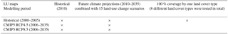
Quantifying how land-use change and climate change affect water resources is a challenge in hydrological science. This work aims to quantify how future projections of land-use and climate change might affect the hydrological response of the Upper Ganges river basin in northern India, which experiences monsoon flooding almost every year. Three different sets of modelling experiments were run using the Joint UK Land Environment Simulator (JULES) land surface model (LSM) and covering the period 2000–2035: in the first set, only climate change is taken into account, and JULES was driven by the CMIP5 (Coupled Model Intercomparison Project Phase 5) outputs of 21 models, under two representative concentration pathways (RCP4.5 and RCP8.5), whilst land use was held fixed at the year 2010. In the second set, only land-use change is taken into account, and JULES was driven by a time series of 15 future land-use pathways, based on Landsat satellite imagery and the Markov chain simulation, whilst the meteorological boundary conditions were held fixed at years 2000–2005. In the third set, both climate change and land-use change were taken into consideration, as the CMIP5 model outputs were used in conjunction with the 15 future land-use pathways to force JULES. Variations in hydrological variables (stream flow, evapotranspiration and soil moisture) are calculated during the simulation period.

Significant changes in the near-future (years 2030–2035) hydrologic fluxes arise under future land-cover and climate change scenarios pointing towards a severe increase in high extremes of flow: the multi-model mean of the 95th percentile of streamflow (Q₅) is projected to increase by 63 % under the combined land-use and climate change high emissions scenario (RCP8.5). The changes in all examined hydrological components are greater in the combined land-use and climate change experiment. Results are further presented in a water resources context, aiming to address potential implications of climate change and land-use change from a water demand perspective. We conclude that future water demands in the Upper Ganges region for winter months may not be met.

1 Introduction

Over recent decades, the Indian subcontinent has undergone some of the largest environmental changes in human history. India's green revolution of widespread implementation of irrigation, application of fertiliser and other modern farming practices, in addition to the ubiquitous benefits, have resulted in large-scale changes in land cover and a significant increase in the exploitation of water resources, including the vast groundwater aquifers of the Gangetic plains. These changes have put severe pressure on water resources – a pressure that is exacerbated further since the increasing demand for a better diet led farmers to mainly plant high-water-intensity crops such as wheat, rice and sugarcane (Kaushal and Kansal, 2011). The country expects double-digit economic growth, whilst the Ganges basin is the most densely populated river basin in the world, with an average population density of 520 persons km⁻². Population density in Uttar Pradesh (which covers a large part of our study area) has increased by more than 100 % from 1971 to 2001, leading to a sharp increase in water demand (Kaushal and Kansal, 2011). Especially during dry periods outside of the summer monsoon season, users of water resources are reliant upon the canals to maintain the required flow levels and sustain riverine ecology. The pressure on water resources is expected to further increase in the near future: for example, by 2030, India's urban population is expected to rise from 286 million (in 2001) to 575 million (Tenhunen and Saavala, 2012).

The Indian monsoon supplies more than 80 % of India's total annual rainfall between June and September (Turner and Annamalai, 2012). The country's population depends largely on the summer monsoon rainfall for food and energy production, agricultural activities and industrial development. Future climate change and particularly the reliance of water resources on the highly erratic precipitation patterns of the summer monsoon pose significant risks to the water supply. Any change in the summer monsoon's timing, intensity and duration, affected by increases in greenhouse gas concentrations, could be detrimental to the water supply. Given the rapid increase in population in the region and the need to improve water and food security, it is essential to understand how the climate will change in the future and how its change will impact humans and the environment.

Over recent years, extreme weather events in South Asia, such as the July 2002 drought over India (Bhat, 2006), the Pakistan floods of July–August 2010 and the north India floods of June 2013, have claimed thousands of lives (Lau and Kim, 2011; Kala, 2014). Several studies, including the IPCC's Fifth Assessment Report (Intergovernmental Panel on Climate Change, AR5; IPCC, 2014), have linked climate change to extreme weather events over South Asia (Singh et al., 2014; World Bank, 2013). Countrywide evidence, supported by localised studies, already suggests a decrease in frequency of light-to-moderate rainfall events and increases in heavy rainfall events, specifically in the central and north-east region of India, since the early 1950s (Dash et al., 2009). The CMIP5 (Coupled Model Intercomparison Project Phase 5) model projections for the end of the 21st century suggest an intensification of heavy precipitation events over India under representative concentration pathway RCP8.5, the “business-as-usual” scenario (Scoccimarro et al., 2013). The average summer monsoon rainfall over India is projected to increase by around 5–10 % (Turner, 2013). In terms of temperature, recent studies based on CMIP5 model projections have shown that heatwaves in India are projected to intensify by the end of the 21st century under RCP8.5, with the Ganges river basin being amongst the areas projected to experience the most severe hazard from extreme heatwaves (Murari et al., 2015; Im et al., 2017).

Understanding and monitoring the hydrologic response of watersheds to land-use and climate change is an important element of water resource planning and management. The quantification of land-use and climate change impacts on hydrological fluxes is a challenge in hydrological science and especially in the data sparse tropical regions. Many studies focus on climate change impacts only and others focus on land-use change impacts only. However, there are just a few studies that consider the combined effects of climate and land-use change by quantitatively integrating both (Karlsson et al., 2016; Pervez and Henebry, 2015; Wang et al., 2014; Zhang et al., 2016). In this study, those relative impacts are investigated by analysing annual variations in hydrological components (stream flow, evapotranspiration and soil moisture) under different land-use and climate change scenarios.

The CMIP5 projections are likely to provide unreliable estimates of the mean values and daily variations in precipitation due to inherent limitations of the general circulation models (GCMs; Raty et al., 2014). Biases have already been identified in simulating the present-day observed Indian summer monsoon climatologies (Sengupta and Rajeevan, 2013). Further, Lutz et al. (2014) found large uncertainties and variations between the annually averaged and seasonal precipitation projections over the Upper Ganges basin. In addition, GCMs were not built for the application of hydrological impact studies. The runoff generation mechanism in GCMs is based on a simplistic representation of the hydrological cycle, and several studies have shown that hydrological models driven directly by GCM model outputs do not perform well (Fowler et al., 2007). To diminish the impacts of GCM biases, several techniques that adjust the climate projections and transform coarse-resolution GCM outputs into finer-scale products suitable for hydrological applications have been developed over recent years and plenty of studies have revised and evaluated these techniques (Fowler et al., 2007; Maraun et al., 2010; Teutschbein and Seibert, 2012; Raisanen and Raty, 2013; Raty et al., 2014). In this study, we applied the delta-change method to observed meteorological datasets. This is a relatively simple approach, broadly used for transforming coarse-resolution GCM outputs into finer-scale products suitable for hydrological applications. The delta-change method was selected as it is a relatively straightforward to apply technique, it is computationally efficient and can be applied to all variables. However, it also has a number of limitations: (a) it assumes a constant delta for each month, as it suggests that relative change is better simulated than absolute values; (b) it assumes a constant spatial pattern of the climatic variable and ignores changes in variability, as the calculated change factors (CFs) only scale the mean, maximum and minimum values; and (c) there is no change in the temporal sequence of wet and dry days (Fowler et al., 2007).

The delta-change method was applied on CMIP5 model outputs and observations to generate future climate scenarios, which were then used to run JULES (Joint UK Land Environment Simulator) and quantify the impact of climate change on the hydrology of the Upper Ganges river basin. The impact of land-use change was quantified by running JULES with a time series of 15 future land-use pathways, based on Landsat satellite imagery and the Markov chain simulation (see Sect. 3), whilst the meteorology was held fixed. Further, the combined impact of climate change and land-use change is examined by using the delta-change transformed observations along with the future land-use pathways. The modelling period up to 2035 was selected as the most relevant for current water resources management decisions. The entire set of available daily CMIP5 model outputs under the historical, RCP4.5 and RCP8.5 experiments was used to cover the range of plausible uncertainty.

The following hypothesis is driving this research: the combined impacts of land-use and climate change on hydrological fluxes will be greater than the impacts posed by land-use change and climate change individually.

The rest of this paper is structured as follows. After describing the study area in Sect. 2, we describe the modelling tools and methods applied in Sect. 3, present the results derived in Sect. 4 and then discuss our findings in Sect. 5, before concluding in Sect. 6. Two appendices included at the end of the paper provide additional material on (a) the CMIP5 projection analysis and (b) the hydrological modelling outputs.

2 Study area

The study area corresponds to the main upper branch of the Ganges and covers an area of 87 000 km². The domain is located in northern India between longitudes 77 to 81^∘ E and latitudes 25 to 32^∘ N. Elevation ranges from 7400 m in the Himalayan mountain peaks to 90 m in the plains (Fig. 1). The Upper Ganges basin lies in the states of Uttarakhand (formerly known as Uttaranchal) and Uttar Pradesh, and the main physical subdivisions of the area are the northern mountainous regions (Himalayan foothills) and the Gangetic plains. In the upstream mountainous regions where the river originates, hydropower is the main focus of development with mega and micro projects either already operating or currently under construction (Bharati et al., 2011). When the river reaches the plains, it becomes subject to vast irrigation demands as more than 410 million people are depending on it to cover their daily needs (Verghese, 1993).

Figure 1 Location map of the study area in north India and a digital elevation model (DEM) of the Upper Ganges basin showing the ranges of the elevations (m altitude). Kanpur barrage was used as the outlet point.

As shown in Fig. 2, areas in the north of the Upper Ganges basin (Himalayas) are either barren or covered by snow. The central and northern parts of the catchment are dominated by forests (20 % of the total catchment area). Around 60 % of the basin is occupied by agriculture (main crop types include wheat, rice, maize, sugarcane, pearl millet (also known as bajra) and potato). Most of the urban and agricultural areas in the basin are located towards the south, in the plains of the Upper Ganges basin.

The annual average rainfall in the Upper Ganges basin ranges between approximately 610 and 1810 mm (Fig. 2). The main source of rainfall is the south-west monsoon, which occurs at this location from July to late September, providing more than 80 % of the total annual precipitation (Turner and Annamalai, 2012). The runoff regime in the Upper Ganges basin is rain-dominated, due to the monsoon-dominated precipitation regime, and the maximum discharge of the river occurs during the monsoon period (Lutz et al., 2014). However, the fluctuation between monsoon flows and dry period flows is very high and that means that large areas are subjected to floods and/or droughts every year (Jain et al., 2007), resulting in significant loss of life and property (e.g. recent northern India floods in Uttarakhand, June 2013).

Since this study is interested in large-scale surface water – climate fluxes and feedbacks – the mountainous headwaters in the north of the basin are not taken into consideration. Although climate change impacts on glaciers and snow melt are of great concern, they are an intensive field of research but have only limited impact on the water resources of the lower plains (Immerzeel et al., 2010). The large downstream monsoon-dominated system of the Ganges river basin, in combination with limited upstream precipitation and small glaciers is the reasons for this minor contribution of snow and glacier water to the Ganges (Immerzeel et al., 2010).

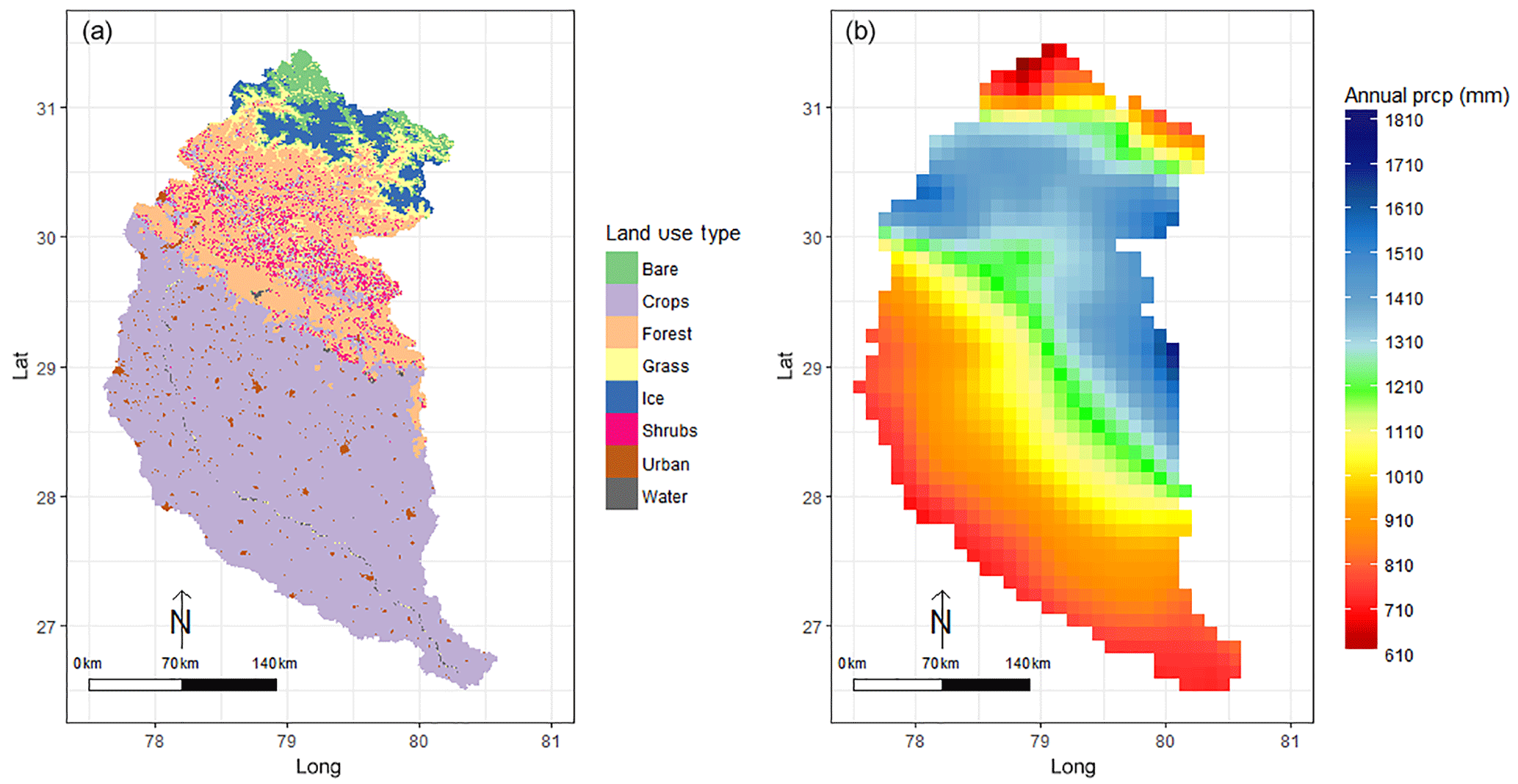
Figure 2 (a) Land-cover map of the Upper Ganges basin, for the year 2010, as developed by Tsarouchi et al. (2014). Landsat 7 ETM+ images for October 2010 were acquired from the US Geological Survey Global Visualization Viewer. The images were co-registered to the UTM projection zone 44N, WGS 1984 datum, and corrected for radiometric and atmospheric effects. They were subsequently classified using a maximum likelihood classifier method with pixel training datasets, resulting in a land-cover map of eight different classes. For more information see Tsarouchi et al. (2014). (b) Annual average precipitation distribution in the study area, based on the TRMM 3B42v7A satellite product (years 1998–2011).

3 Modelling tools and methods

3.1 Future climate projection data from CMIP5

GCM outputs from 21 models of the CMIP5 multi-model database were obtained through the UK Centre for Environmental Data Analysis (CEDA). All meteorological variables required by JULES (i.e. time series of incoming short-wave and long-wave radiation, temperature, specific humidity, wind speed and surface pressure) were acquired from the historical, RCP4.5 and RCP8.5 experiments of 21 CMIP5 models. RCP4.5 and RCP8.5 were chosen because they correspond to contrasting future greenhouse gas emissions scenarios: RCP4.5 represents a “middle-of-the-road” scenario, in which the projected change in global mean surface air temperature for the late 21st century (2081–2100) relative to the reference period of 1986–2005 is 1.8 ^∘C; RCP8.5 represents a business-as-usual scenario of future emissions, where the projected change in global mean surface air temperature for the late 21st century relative to the reference period of 1986–2005 is 3.7 ^∘C (IPCC, 2013).

To run JULES, we used CMIP5 model outputs covering the years 2000–2005 from the historical experiment, whilst from the RCP4.5 and RCP8.5 experiments we used model outputs covering the years 2006–2035. The delta-change method was applied on the CMIP5 model outputs and observations to generate future climate scenarios. This method calculates the change in time between the control and future simulations of a variable and applies this change in the baseline (observed) climate by simply adding or scaling the mean climatic change factor to each day (Fowler et al., 2007). The CF indicates relative change for fluxes exchanged between the atmosphere and surface in order to avoid negative values and absolute change for state meteorological variables. So, for precipitation, radiation and wind speed, the monthly CF is calculated as

$$\begin{array}{}\text{(1)}& \mathrm{CF}={\displaystyle \frac{{\stackrel{\mathrm{‾}}{V}}_{\mathrm{fut}}}{{\stackrel{\mathrm{‾}}{V}}_{\mathrm{hist}}}},\end{array}$$

where $\stackrel{\mathrm{‾}}{V}$ is the monthly climatological mean for a given flux variable. For temperature, pressure and specific humidity, which are state variables, the CF is calculated as

$$\begin{array}{}\text{(2)}& \mathrm{CF}={\stackrel{\mathrm{‾}}{V}}_{\mathrm{fut}}-{\stackrel{\mathrm{‾}}{V}}_{\mathrm{hist}}.\end{array}$$

As baseline (observed) climate, we used for precipitation the Tropical Rainfall Measuring Mission (TRMM) Multi-satellite Precipitation Analysis (TMPA) product, version 7, (Huffman et al., 2007; Huffman and Bolvin, 2013), hereafter referred to as TRMMv7; and for the rest meteorological variables data were obtained from the Princeton hydrology archive and consist of reanalysis data that have been post-processed and merged with observations (National Centers for Environmental Prediction, Kalnay et al., 1996; Sheffield et al., 2006). The mean climatic CFs were based on monthly-mean climatological conditions over 6-year time slices from each of the 21 CMIP5 models: 2000–2005 for the historical CMIP5 model outputs and 2006–2035 for RCP4.5 and RCP8.5. The CFs were used to rescale the historical observations at the daily timescale. The CFs were further interpolated to the 0.1^∘ resolution of the modelling setup, using the bilinear interpolation method.

3.2 Pathways of future land-use change

For the future pathways of land-use change, 15 maps for years up to 2035 were developed in Tsarouchi et al. (2014), based on Landsat satellite imagery and the Markov chain simulation. Under the assumption that the drivers that caused land-use changes in recent years (2000–2010) will remain the same in the nearby future (years up to 2035), 15 transition probability matrices indicating transition potentials from one land-use type to another where generated. These 15 transition matrices are based on historic land-use transitions that occurred during the period from 2000 to 2010, for which 6 land-use maps were available (one map every 2 years). The 15 matrices describe all possible land-use transition combinations of the years 2000, 2002, 2004, 2006, 2008 and 2010 (e.g. 2000–2002, 2000–2004, 2000–2006). The trends in different matrices vary and this is also reflected in the future projections (i.e. they are not exactly the same).

Before developing the future pathways of land-use change, we tested the method in a previous study, over the same area, to examine its accuracy (Tsarouchi et al., 2014). As a validation measure of the ability to generate future pathways under the Markov chain analysis, we used transition matrices of years previous to 2010 and generated maps for the year 2010. These maps were then compared to the historical land-cover map of 2010. The results showed that the generated maps for 2010 were not very different compared to the historical map of 2010. Highest overall uncertainties were observed for the forest and shrubs land-use types. For example, the proportion of forest in the historic 2010 map was 17.12 %, while the two most extreme values of forest coverage that we obtained through the Markov chain analysis were 19.98 and 15.20 %. This gave us confidence to apply the same method for developing other near-future scenarios.

Figure 3 highlights the spread of these 15 future pathways for the year 2035 and how their land-cover proportions compare to the historic year 2010. The variations between the different pathways are not large and the main trends of change identified are forest growth, urbanisation and on the other hand loss of bare soil, grasslands and shrubs. All 15 possible combinations were used in this study, because there was no straightforward way to select a single or a few of the projections as more representative of future change. By keeping all 15 scenarios, we obtain a good indication of the uncertainties associated with developing scenarios of future change and their often contrasting impacts on hydrological variables. For a more detailed description of the method used to generate the future land-use pathways see Tsarouchi et al. (2014).

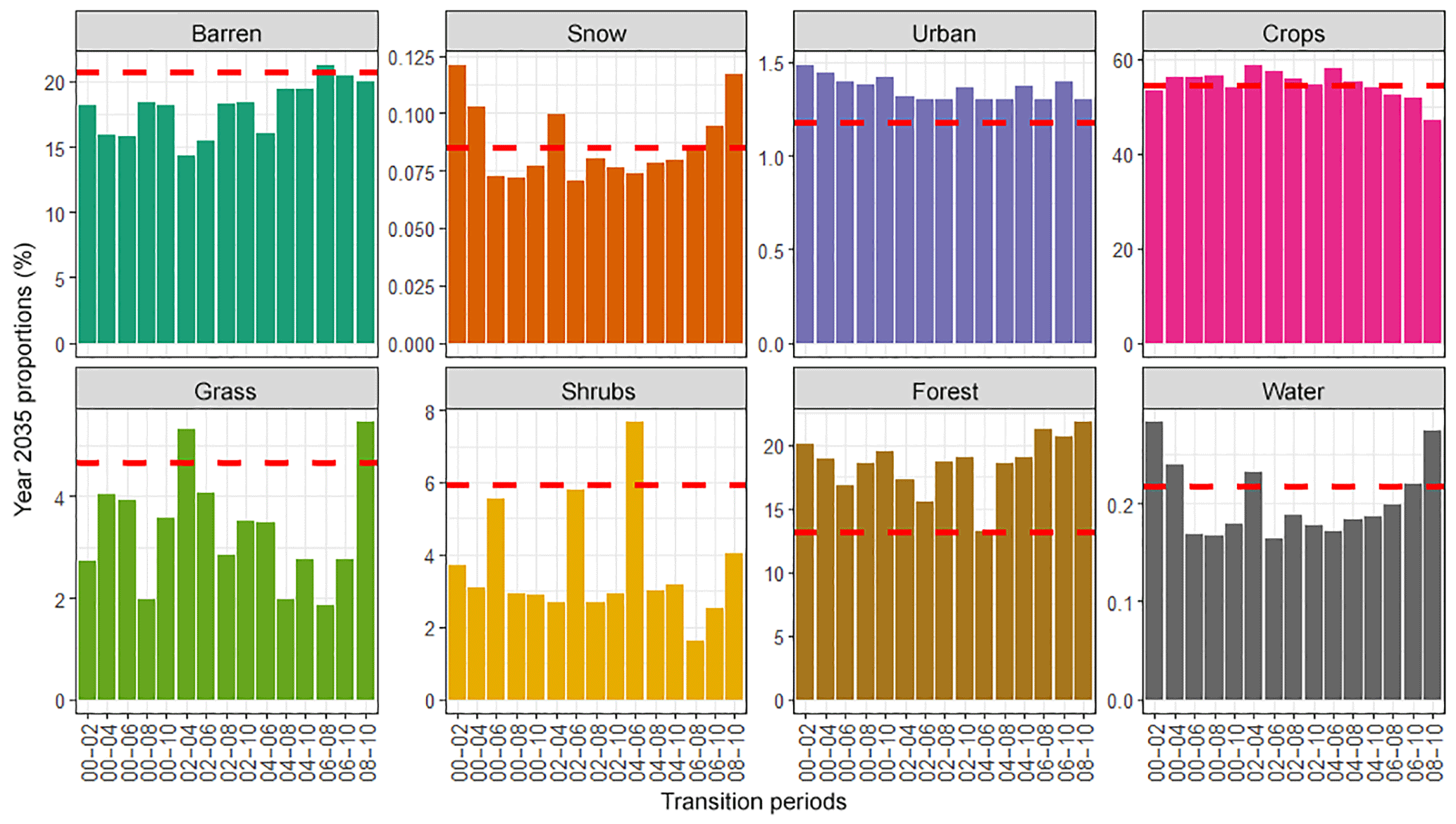
Figure 3 Plots indicating the different land uses for year 2035, amongst the 15 land-use pathways developed by applying the Markov chain simulation in Tsarouchi et al. (2014). The x axis indicates the transition period used to calibrate the Markov chain model; for instance, “00–02” refers to the historical period 2000–2002. The red line illustrates the actual land-cover proportions of year 2010, as derived from the Landsat classifications.

3.3 The JULES land surface model

In this study we use the Joint UK Land Environment Simulator (JULES, version 3.4) land surface model (LSM) (Best et al., 2011) in order to investigate the impact of land-use change and climate change in hydrological fluxes of the Upper Ganges river basin. We drive the model with delta-change transformed climate projections from the CMIP5 multi-model database and a series of future land-use pathways, based on Landsat satellite imagery and the Markov chain simulation.

JULES was developed by the UK Met Office and is based on MOSES (Met Office Surface Exchange System), the LSM used in the Unified Model of the UK Met Office. It is a combined process-based distributed and lumped parameter model that simulates the exchange of energy, water, and carbon fluxes between land surface and the atmosphere. The input meteorological data requirements are time series of incoming short-wave and long-wave radiation, temperature, specific humidity, wind speed and surface pressure. These are used in a full energy balance equation that includes components of radiation, sensible heat, latent heat, canopy heat and ground surface heat.

The model partitions precipitation into canopy interception and throughfall. In the default runoff scheme, surface runoff is generated based on Hortonian infiltration. Surface heterogeneity within JULES is represented by the tile approach (Essery et al., 2003). The surface of each grid-box comprises fractions of nine different land-cover types: five vegetated plant functional types – broad-leaf trees, needle-leaf trees, C₃ grasses, C₄ grasses and shrubs; and four non-vegetated – urban, water, bare soils and ice. For each surface type of the grid-box, the energy balance is solved, and a weighted average is calculated from the individual surface fluxes for each grid-box. In the subsurface, the soil column is divided into four layers, which have a thickness of 0.1, 0.25, 0.65 and 2 m respectively, from the top to the bottom. The Darcy-Richards equation (Richards, 1931) is solved using a finite difference approximation to calculate water movement through the soil. Subsurface runoff is represented by a free drainage from the deepest soil layer. The soil water retention characteristics (relationship between volumetric water content and soil suction) and the relationship between volumetric water content and hydraulic conductivity follow the relationships of van Genuchten (1980). For a more detailed description of the model see Best et al. (2011).

JULES was run in a 0.1^∘ longitude × 0.1^∘ latitude grid resolution for the period 2000–2035. For each grid point, the full set of input data (model parameters, time series of meteorological data, land use and soil map) were prescribed. Before each run of the model, a spin-up run is performed to initialise the internal states. For the parametrisation of plant functional types and non-vegetated tiles, the default parameters described in Tables 5 and 6 of Best et al. (2011) were used.

The model was forced with the rescaled historical observations to generate future hydrological projections for the Upper Ganges basin that go up to year 2035. Three different sets of modelling experiments were run: in the first one, only climate change was taken into account, as JULES was driven by the CMIP5 outputs of 21 models, under two emission scenarios (RCP4.5 and RCP8.5), but land use was held fixed at year 2010 (see Sect. 3.2). In the second one, only land-use change was taken into account, by driving JULES with a set of 15 year-to-year varying time series of future land-use pathways, whilst the driving meteorology was held to historical levels. In addition, the model was driven by eight extreme pathways where we have assumed 100 % coverage of the study area by one land-cover type, whilst again the driving meteorology was held to historical levels. In the third set, both climate change and land-use change were taken into consideration, as, apart from the CMIP5 model outputs, JULES was also forced by the set of 15 year-to-year varying time series of future land-use pathways. The impact of both climate change and land-use change on the future hydrological variables of the study area is examined. Table 1 outlines all of the JULES runs as described above.

In the following sections, the subscript cl corresponds to results produced by taking only climate change into account, over the simulation period 2030–2035; the subscript cl_lu corresponds to results produced by taking into account both climate change and land-use change, over the simulation period 2030–2035; and the subscript hist corresponds to results from the historical simulation period 2000–2005.

Table 1 Summary of the JULES experiments.

3.4 Water demand data

Aiming to place our results in a future water resources context (focusing on the period 2030–2035), we use water demand data from a recent study by Sapkota et al. (2013). The mean monthly water demands shown in Fig. 4 of Sapkota et al. (2013) are used in combination with future projections of changes in India's water demands, as presented in the study by Amarasinghe et al. (2007). The latter study suggests an expected 8 % increase in surface water demand for irrigation, 130 % increase in surface water demand for domestic usage and 152 % increase in surface water demand for industrial usage by 2030 under a business-as-usual scenario, which is mainly extrapolating trends of recent years (calculations after linearly interpolating results presented for years 2025 and 2050).

4 Results

4.1 CMIP5 projection analysis

A direct analysis of the monthly precipitation climatologies for the Upper Ganges basin reveals large variations between the different GCM precipitation datasets (Fig. 4). Interestingly, there are models that are not able to capture at all the seasonal cycle and the summer monsoon precipitation, but instead reproduce a flat annual climatology (likely due to poor representations of the annual cycle of monsoon circulation). This illustrates the large uncertainties and questions the ability of some of the models to represent the present-day climate in the study area. However, this is no straightforward indicator of their ability to generate reasonable future climate projections (Liang et al., 2008).

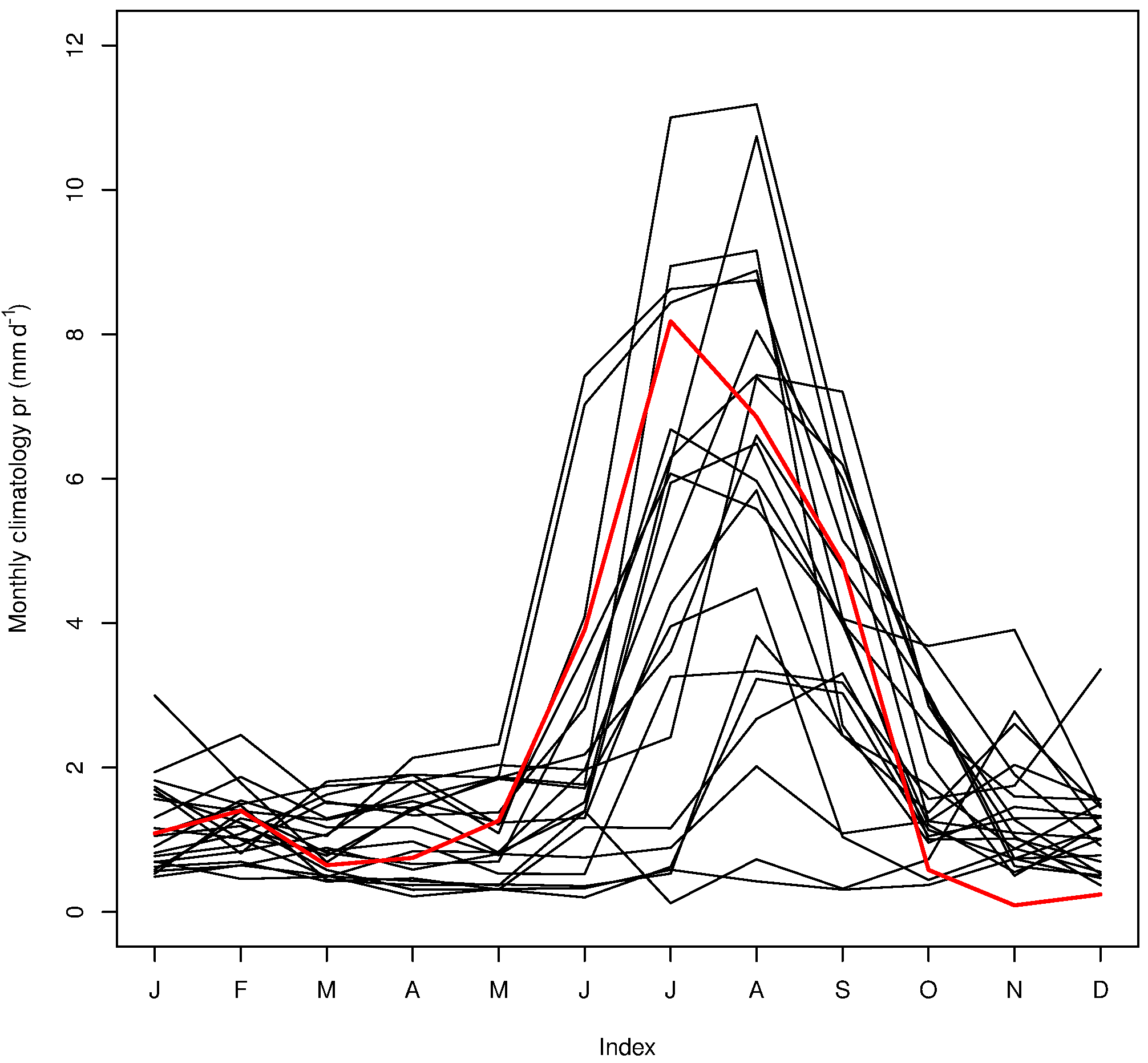
Figure 4 Monthly historical precipitation climatologies of the 21 CMIP5 models used in this study (black) and how they compare to the TRMMv7 satellite product (red), over the period 2000–2005 (the CMIP5 historical experiment ends in 2005). The data correspond to areal averages, covering the extent of the Upper Ganges basin.

Figure 5 shows the CFs of precipitation relative to the historic period 2000–2005, averaged in the Upper Ganges basin. It is evident that the spread of the results is large, and many models show opposite directions of change. Nevertheless, all the mean values point towards an increased precipitation for all months. The uncertainty is higher for the dry months of November and December, which have the highest percent increase in precipitation relative to historic values. On the other hand, the spread seems to be narrower for the wet summer months but nonetheless there are still models with contrasting results.

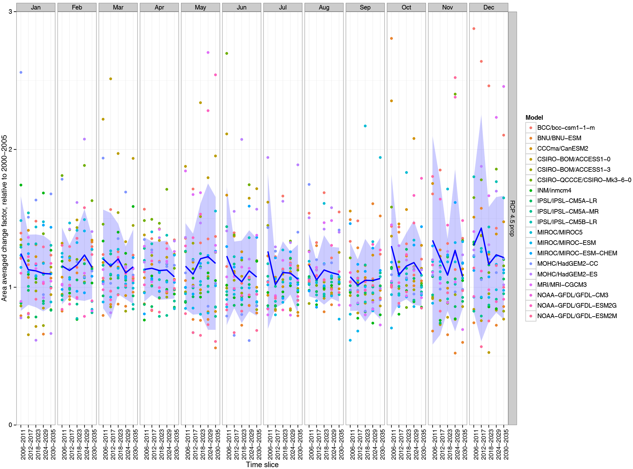
Figure 5 Six-year CFs of precipitation in the Upper Ganges basin. Each dot represents the basin's areal average of a particular model. The precipitation anomalies are relative, unitless values. A higher than 1 value indicates an increase and a smaller than 1 value indicates a decrease in precipitation. The blue line represents the mean value whereas the shading represents the spread of projections from the multi-model ensemble.

Further details on the skill of the CMIP5 GCM models used in this study are available in Appendix Appendix A.

4.2 Hydrological projections

After forcing JULES with the downscaled future climate projections from the CMIP5 multi-model database and in conjunction with estimates of different future land-use pathways, we calculate variations in the following hydrological components: flows at Kanpur barrage, evapotranspiration and soil moisture.

Focusing upon the multi-model mean values (Fig. 6), for the entire Upper Ganges basin, when only climate change is taken into consideration, the high flows exceeded only 5 % of time (Q₅) are projected to increase in magnitude by 41 % (SD = 73, the standard deviation of the percent change) compared to historic values under RCP4.5 and by 60 % (SD = 76) under RCP8.5 (Table 2). When only land-use change is taken into account, different pathways project different types of change for Q₅: one of the pathways (08–10) projects an increase of 1.3 % and other pathways project decreases of up to 0.5 %. For low flows, exceeded 95 % of time (Q₉₅), all pathways are projecting a decrease, ranging from 11.8 to 19.5 % (Table 3). The decrease in low flows is possibly due to the combined impacts of forest growth and bare soil loss, which are less surface runoff and more evapotranspiration. These appear to be enough to offset the impacts of urbanisation (i.e. reduced infiltration and increased discharge), which is one of the land-use change trends being projected consistently across all pathways.

When both climate change and land-use change are taken into account, the increase in the high extremes of flows is slightly higher: 42 % (SD = 72) increase under RCP4.5 and 63 % (SD = 72) increase under RCP8.5. In the low flows, the impact of climate change only is not as significant: Q₉₅ is decreased in magnitude by 2 % (SD = 28) under RCP4.5 and by 3 % (SD = 19) under RCP8.5. When land-use change is also taken into account, Q₉₅ is projected to increase by 1 % (SD = 31) under RCP4.5 and to decrease by 1 % (SD = 17) under RCP8.5. So there is a clear impact of both climate change and land-use change in the high and low extremes of flows.

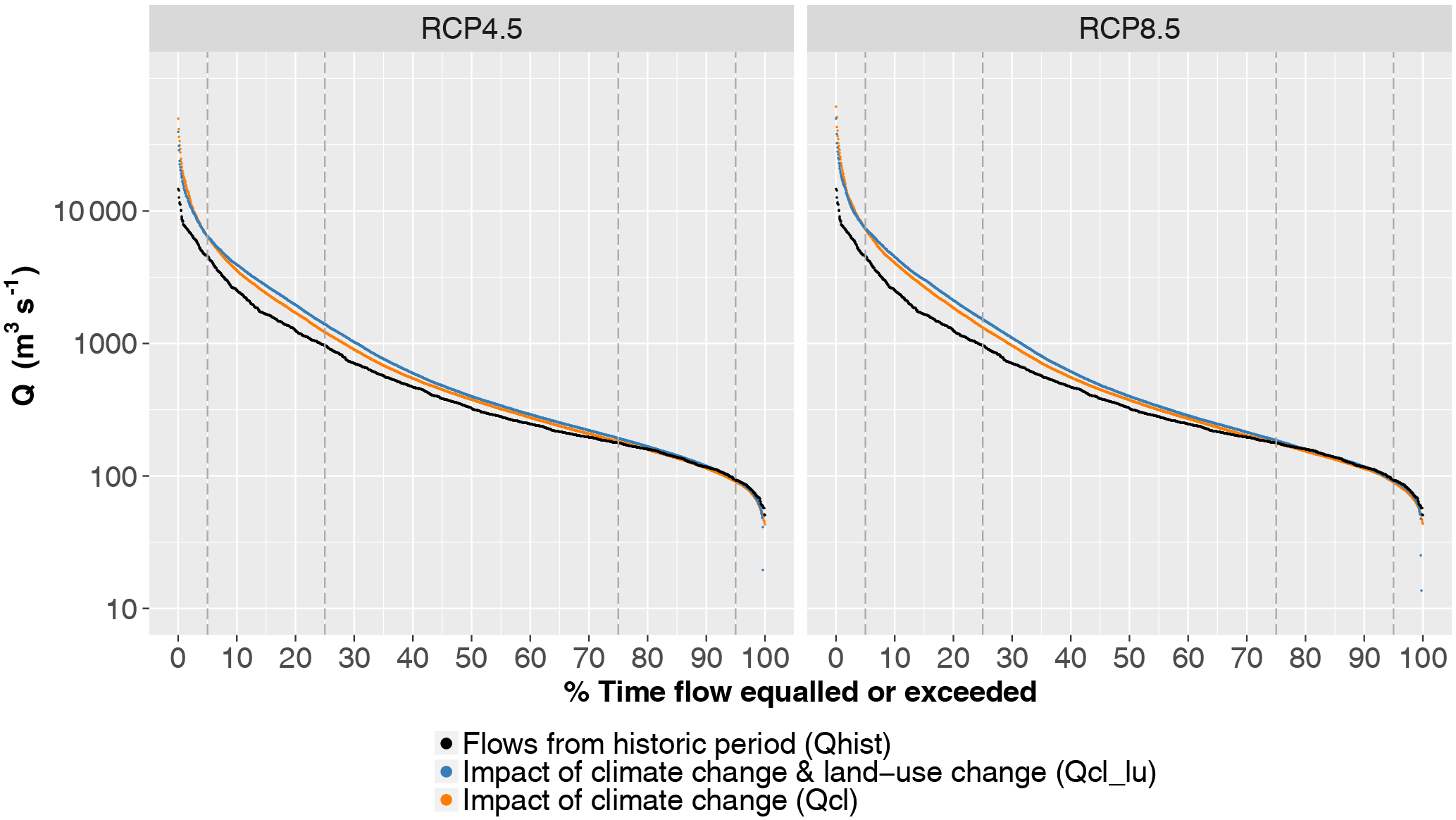
Figure 6 Flow duration curves of the streamflows simulated by JULES for the Upper Ganges basin, at Kanpur barrage. Orange: multi-model mean values when only climate change is taken into account (Q_cl); simulation period 2030–2035. Blue: multi-model mean values when both climate change and land-use change are taken into account (Q_{cl_lu}); simulation period 2030–2035. Black: historical period (Q_hist); simulation period 2000–2005.

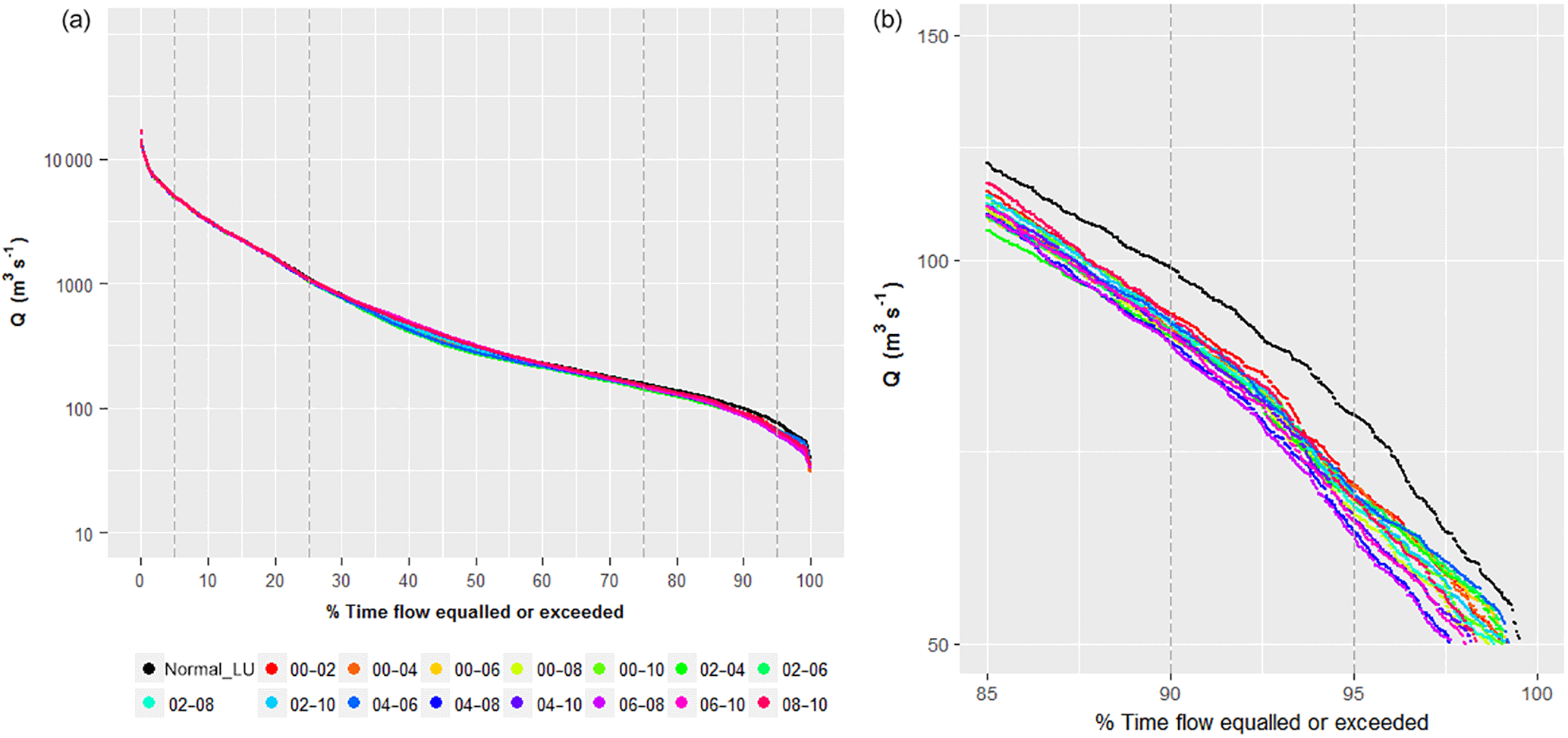
Figure 7 (a) Flow duration curves of the streamflows simulated by JULES for the Upper Ganges basin, at Kanpur barrage, for each of the 15 different future projections of land use. The meteorology was held fixed, so that only the impact of land-use change can be examined. For reference, the results of the run with the 2010 land-cover map are also plotted (normal_LU). (b) Plot focusing on the low flows, which are mostly affected by differences in the land cover.

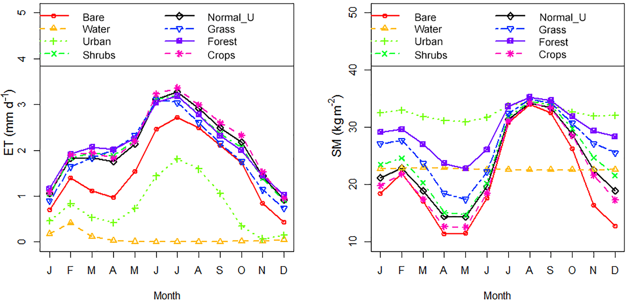
Figure 8 Evapotranspiration and soil moisture climatologies under the assumption that the study area was 100 % covered by a particular land-cover type. For reference, the results of the run with the 2010 land-cover map are also plotted (normal_LU).

Figure 9 Percent change in evapotranspiration and soil moisture climatologies when running JULES with each of the 15 different future projections of land use, relative to the 2010 land-cover map. The meteorology was held fixed, so that only the impact of land-use change can be examined.

Table 2 Q₅ and Q₉₅ flow values (m³ s⁻¹) based on the flow duration curves shown in Fig. 6.

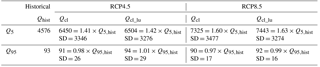
Table 3 Percent change in Q₅ and Q₉₅ flow values, relative to the run with the 2010 land-cover map, based on the flow duration curves shown in Fig. 7.

Figure 10 Absolute changes in spatial evapotranspiration (ET) fluxes between the historical simulation period 2000–2005 and the future projection simulation period 2030–2035 for the Upper Ganges basin and for each of the emission scenarios (RCP4.5 and RCP8.5). Results are split into 3-month period seasonalities for winter (DJF), spring (MAM) and summer (JJA) under the two types of experiments: (a) only climate change is taken into account (ETcl) and (b) both climate change and land-use change are taken into account (ETcl_lu).

Spatial changes in evapotranspiration between the historical (2000–2005) and future projection period (2030–2035), under both emission scenarios (RCP4.5 and RCP8.5), are shown in Fig. 10. Results are split into 3-month period seasonalities for winter (DJF), spring (MAM) and summer (JJA) under the two types of experiments: (a) only climate change is taken into account (ET_cl) and (b) both climate change and land-use change are taken into account (ET_{cl_lu}). The differences between ET_cl and ET_{cl_lu} are very small in all seasons examined. The highest increase in evapotranspiration (0.8 mm d⁻¹) is projected to occur during spring in the southern agricultural parts of the catchment. The highest decrease in evapotranspiration (−0.9 mm d⁻¹) is projected to occur during the spring and summer periods in the mid-north parts of the study area. Nonetheless, those changes are cancelled out when spatially averaged across the catchment (Figs. 12 and B4).

The impact of land-use change on evapotranspiration and soil moisture is illustrated in Figs. 8 and 9. In terms of evapotranspiration, the model results by using the 2010 land-cover map are similar to model results when the land is 100 % covered by forest, grass, crops or shrubs (Fig. 8). When the land cover is 100 % bare soil, urban areas or water, evapotranspiration is reduced as there is no transpiration. In these cases, evaporation takes the form of bare soil evaporation (restricted by water availability at the surface), evaporation from open water surfaces or ponding for urban surfaces. When the model was run with the 15 different land-use pathways and the outputs compared against the 2010 land-cover map model outputs, the changes are of the order of ±1.9 %.

For soil moisture, the model results by using the 2010 land-cover map are similar to model results when the land is 100 % covered by crops or shrubs (Fig. 8). In the warm MAM period, which follows the dry DJF months, the upper soil layer is likely dryer because of strong evaporation. During the monsoon rainfall period (JJA), the soil moisture content is increasing. The soil moisture sensitivity to different land-cover types is larger on the dry season than on the wet season. In JULES, vegetation roots are assumed to enhance the maximum surface water infiltration rate by a factor of 4 for forests and 2 for grass, shrubs and crops. When we run the model with the 15 different land-use pathways, again the sensitivity is larger on the dry season, with pathway 08–10 showing the highest increase relative to the baseline run (6.8 % for April) and scenario 04–06 the only pathway showing a decrease (−1.8 % for April). For pathway 04–06, the decrease in dry season soil moisture could be due to the higher proportion of crops in the study area that are accessing the top layer water content, in combination with lower proportions of water and snow coverage. For pathway 08–10, the increased soil moisture in the dry season could be due to the increased forest and grass cover and higher infiltration rates associated with them.

In terms of spatial changes in soil moisture, it is shown in Fig. 11 that, similarly to the patterns of evapotranspiration change, the highest increase in multi-model mean soil moisture (4 kg m⁻²) is projected to occur during spring in the southern agricultural parts of the catchment. The highest decrease in soil moisture (−10 kg m⁻²) is projected to occur during the winter and summer periods in the mid-north parts of the study area. However, it seems that these changes in soil moisture are cancelled out when spatially averaged results are calculated in Figs. 13 and B5.

Note that for the projections of evapotranspiration and soil moisture fluxes, the differences between the two RCP scenarios are not large. In the nearby-future period examined here (2030–2035), the relative importance of the RCPs is far smaller than the GCM model uncertainties.

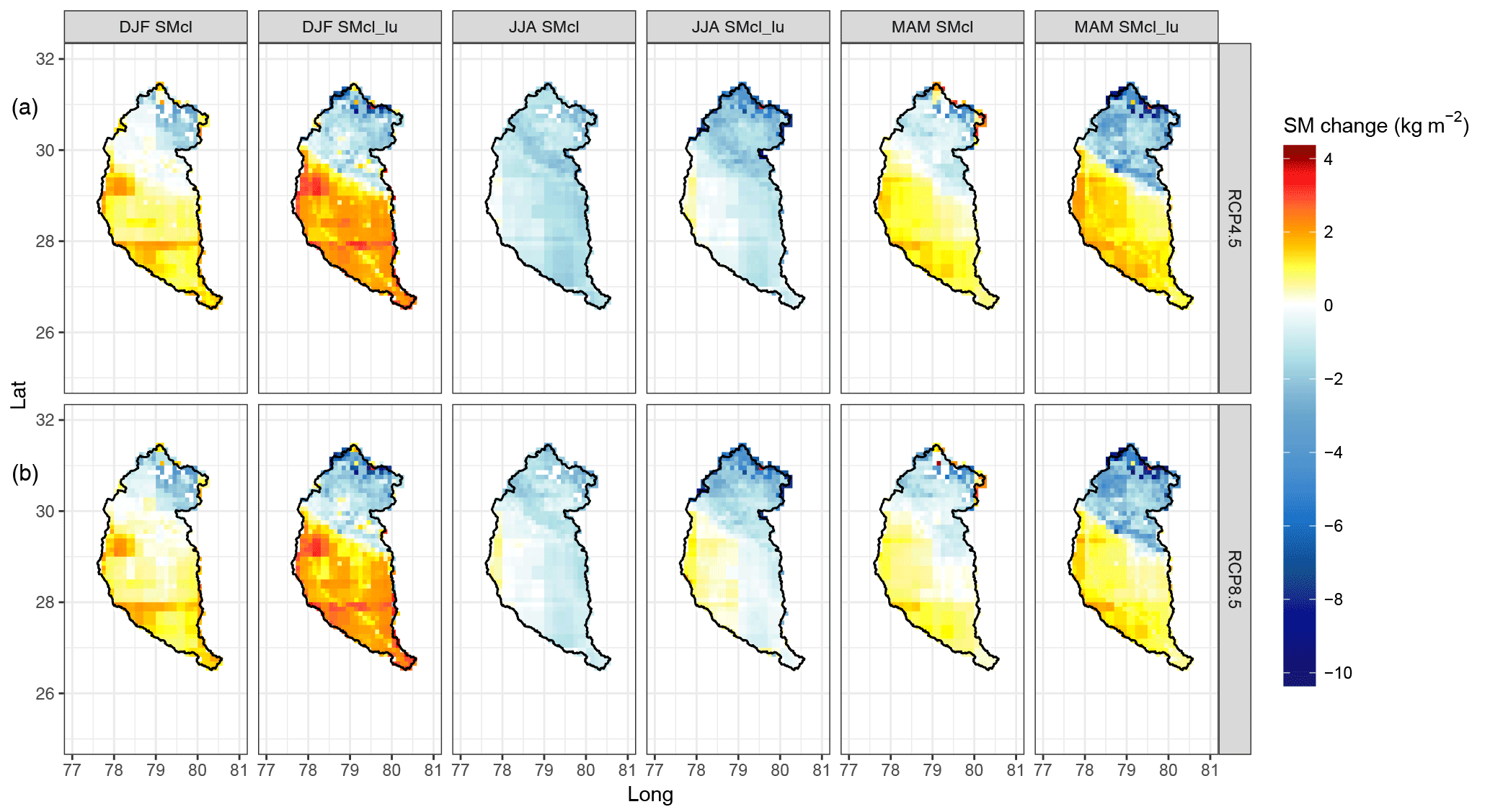
Figure 11 Absolute changes in spatial soil moisture (SM) fluxes between the historical simulation period 2000–2005 and the future projection simulation period 2030–2035 for the Upper Ganges basin and for each of the emission scenarios (RCP4.5 and RCP8.5). Results are split into 3-month period seasonalities for winter (DJF), spring (MAM) and summer (JJA) under the two types of experiments: (a) only climate change is taken into account (SMcl) and (b) both climate change and land-use change are taken into account (SMcl_lu).

Further details on the hydrological projections developed for this study are available in Appendix Appendix B.

5 Discussion

This section places our results in a water resources context, by discussing the implications of climate change on the water resources of the Upper Ganges and whether it is likely that water demand thresholds (i.e. amount of water that sustains environmental flows and water consumption) of the region will be exceeded in the future. A recent study by Sapkota et al. (2013) presented mean monthly water demands for irrigation, industrial and domestic purposes (period 1991–2005) in the Upper Ganges basin. According to this study, irrigation water demands from canals (which are much higher compared to industrial and domestic demands) are low during the monsoon period from June to September and high from November to February. During the winter months of December and January, water demand in the Upper Ganges basin is already unmet. In recent years, pressure has increased on the river canals to maintain flows during the dry season, due to the introduction of high-water-intensity crops, agricultural expansion and population growth (Sapkota et al., 2013).

Figure 12 Multi-model mean values of the evapotranspiration (ET) fluxes simulated by JULES for the Upper Ganges basin and for each of the emission scenarios (RCP4.5 and RCP8.5). Black colour corresponds to the historical simulation period 2000–2005 (ET_hist). Orange colour corresponds to the simulation period 2030–2035, when only climate change is taken into account (ET_cl). Blue colour corresponds to the simulation period 2030–2035, when both climate change and land-use change are taken into account (ET_{cl_lu}). Shaded areas correspond to the maximum and minimum evapotranspiration values obtained from different GCM forcings and illustrate the large CMIP5 model spread.

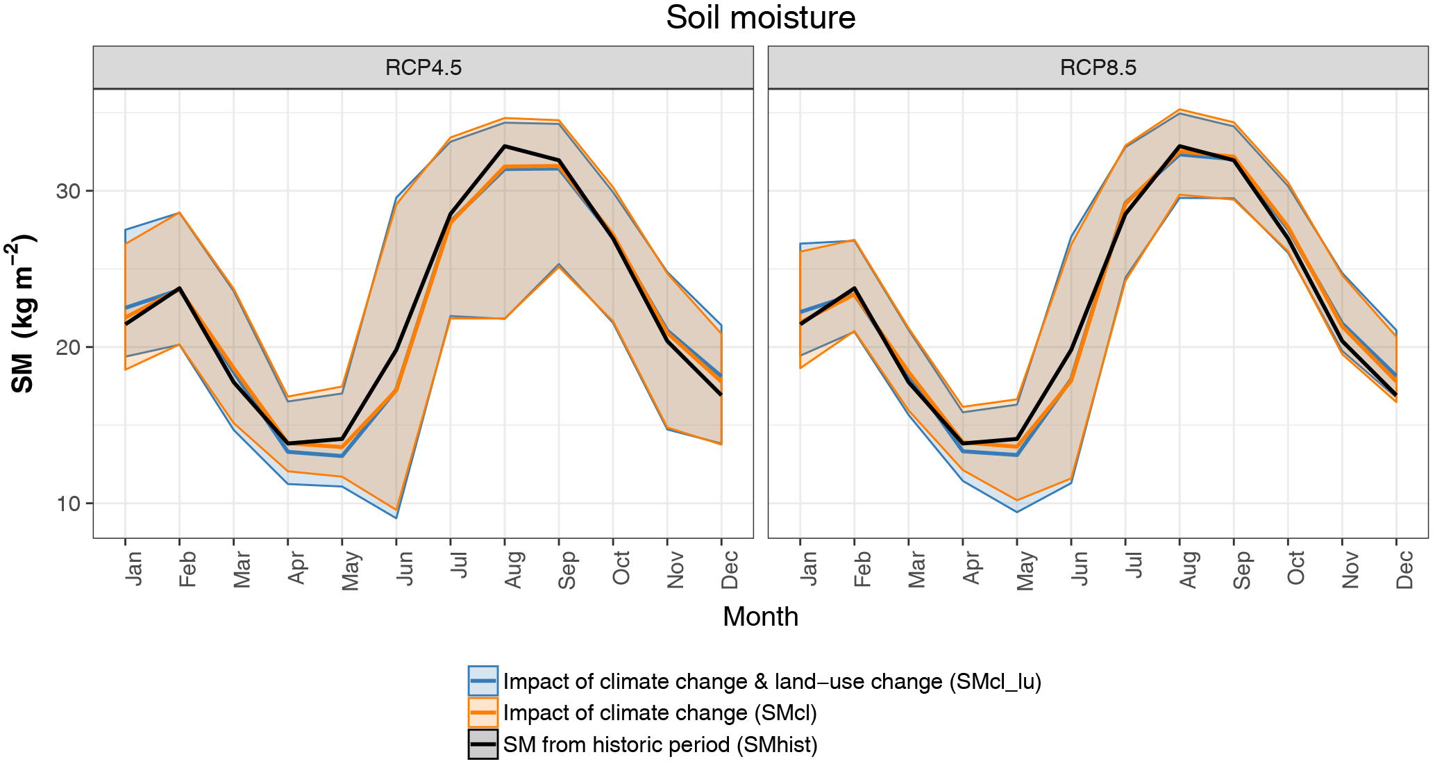
Figure 13 Multi-model mean values of the soil moisture fluxes simulated by JULES for the Upper Ganges basin and for each of the emission scenarios (RCP4.5 and RCP8.5). Black colour corresponds to the historical simulation period 2000–2005 (SM_hist). Orange colour corresponds to the simulation period 2030–2035, when only climate change is taken into account (SM_cl). Blue colour corresponds to the simulation period 2030–2035, when both climate change and land-use change are taken into account (SM_{cl_lu}). Shaded areas correspond to the maximum and minimum soil moisture values obtained from different GCM forcings and illustrate the large CMIP5 model spread.

Based on the studies by Amarasinghe et al. (2007) and Sapkota et al. (2013) and as described in Sect. 3.4, future projections of surface water demand for the Upper Ganges basin were generated on a monthly basis and for the period 2030–2035. Figure 14 shows how the future expected surface water demand compares with the flow volumes as calculated by JULES (period 2030–2035) under the two examined RCP scenarios, when only climate change is taken into account and when both climate change and land-use change are taken into account. Since the main months under water stress are those in the dry season, and in order to better visualise the results outside the wet summer period (which is dominated by high flows), the y axis was limited to values lower than 2000 million m³ of water. The future winter months (December–February) are expected to be the most problematic in terms of meeting the surface water demands, with agriculture being the main water user. This poses threats to the river's capacity to maintain flows at an acceptable ecological level (environmental flows) during those months. Sapkota et al. (2013) showed that using lower-water-intensity crops in the Upper Ganges basin is more efficient than reducing the total agricultural area by 40 % in reducing the unmet irrigation water demands.

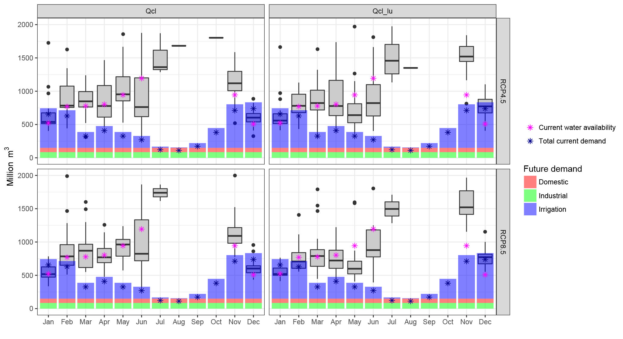
Figure 14 Bars showing future projections of monthly surface water demand for irrigation, domestic and industrial usage, during the period 2030–2035, for the Upper Ganges basin. Box plots indicate monthly flow volumes calculated by JULES under different GCM forcings for the same period. The demand data are based on figures presented in the studies by Sapkota et al. (2013) and Amarasinghe et al. (2007), as discussed above.

One of the limitations of the present study is that the data used in the JULES experiments and in the water demand analysis are not fully consistent with each other in all cases. Land-use projections across RCP 4.5 and 8.5 vary substantially. In RCP8.5, developing countries experience net increases in agricultural land and urbanisation, while forest cover declines. In RCP4.5, due to afforestation and reforestation policies the extent of crop and grass land declines and the forested area increases. These RCP assumptions about future land use are not consistent with all 15 land-cover pathways that were used to test the impacts of land-use change in this study. Further, the water demand projections of the Amarasinghe et al. (2007) study are mainly based on the extrapolations of recent-year trends but are not consistent with all 15 land-cover pathways. The water demand projections are consistent with further urbanisation and the assumption of continuous irrigation expansion. Therefore, although the projections to 2035 are not too far ahead, there is always the possibility that the business-as-usual water demand drivers could significantly change, altering the future projections. However, we do identify some consistency with RCP8.5 (which is considered to be a business-as-usual scenario) and also with some of the land-use change trends detected in the 15 pathways used in our study (e.g. urbanisation and agricultural expansion).

Additionally, understanding the future water availability in India is much more complex than looking from the perspective of climate and land-use change only. For instance, India is one of the largest hydropower generators in Asia. A potential future increase in hydropower capacity, aside from its large benefits in terms of reducing carbon emissions, brings further environmental concerns regarding river flows, water quality and eco-diversity. Therefore, the impacts of such water management decisions (e.g. hydropower dam structures) could also play a major role in the water balance of this region. As studies have shown, changing practices within certain types of land use (i.e. increased irrigation efficiency, upstream dams) are potentially more important than land-use change per se in influencing water availability (Calder, 1993; Solín et al., 2011), and this may be the case in the future for the Upper Ganges basin.

Overall, climate change is the main driver of hydrological change in the near-term-future scenarios explored in this study. If no dramatic land-use changes take place in the nearby future, the main alterations in hydrological fluxes are expected to arise from the change in the meteorology (and mainly precipitation). The relative contribution of land-use change is of an approximate magnitude of 2 % change. However, the strong inter-model uncertainties in the future projections (see SD values in Sect. 4.2 and Table 2), which were possibly amplified by the delta-change approach, are posing a limitation to the confidence of these results. Nevertheless, there is qualitative similarity between results shown here and results presented by Lutz et al. (2014), who found that for the Upper Ganges basin, projected precipitation increases during the monsoon period could lead to increases in total annual runoff of up to 10 % for RCP4.5 and 27 % for RCP8.5 during the period 2041–2050. Likewise, Masood et al. (2015) found that, in the near future (2015–2039), under RCP8.5, total runoff in the Ganges basin is projected to increase by 2.5 % in the dry season (November–April), by 12.1 % in the wet season (May–October) and by 11.3 % annually.

As GCM uncertainties are unlikely to decrease quickly, decisions on the adaptation and mitigation of climate change should not be delayed (Knutti and Sedlacek, 2013).

6 Conclusions

In this study, the impact of land-use change and climate change on the future hydrology of the Upper Ganges basin was assessed by calculating annual variations in hydrological components (stream flow, evapotranspiration and soil moisture). Three sets of modelling experiments were run in the JULES land-surface model, covering the period 2000–2035: (a) the model was forced with future climate projections from the CMIP5 multi-model database, whilst land use was held fixed at year 2010; (b) the model was forced with 15 future land-use pathways, based on Landsat satellite images and the Markov chain simulation, whilst the meteorology was held fixed; and (c) the model was forced with future climate projections from the CMIP5 multi-model database, in conjunction with the 15 future land-use pathways.

Large variations between GCM-derived precipitation datasets arise from a basic analysis of CMIP5 model outputs. A stronger wet season is projected to occur by the end of the century according to multi-model mean values.

Significant differences between the historic and nearby-future hydrologic fluxes arise under future land-cover and climate change scenarios, pointing towards a severe increase in high extremes of flow. The changes in all examined hydrological components are slightly greater in the combined land-use and climate change scenario compared to the stand-alone climate change scenario. However, the main driver of future hydrological change is climate change. In terms of spatial changes in evapotranspiration and soil moisture, the changes that occur in various parts of the catchment are cancelled out by changes in the opposite direction, occurring in different parts of the catchment, leading to smaller overall changes in terms of areal averages.

The large uncertainties in the CMIP5 model outputs were possibly amplified by the delta-change approach followed here and led to a large spread of results for the future hydrological variables (e.g. Figs. 12 and 13, SD values in Sect. 4.2 and Table 2). Potential inconsistencies between the climate change, land-use change and water demand projections may have added extra uncertainty in some of the modelling outputs and this has been acknowledged in the discussion section. Nonetheless, as GCM uncertainties are unlikely to decrease in the near future, this work could help prioritise adaptation strategies and regional land-use planning to improve northern India's water resources.

Lastly, the results were presented in a water resources context, with the aim of understanding what climate and land-use change mean for the future water resources of the Upper Ganges basin. When looking into future water availability and demand (period 2030–2035), the river's capacity to maintain ecological flows during the dry season is threatened.

Appendix A: CMIP5 projection analysis

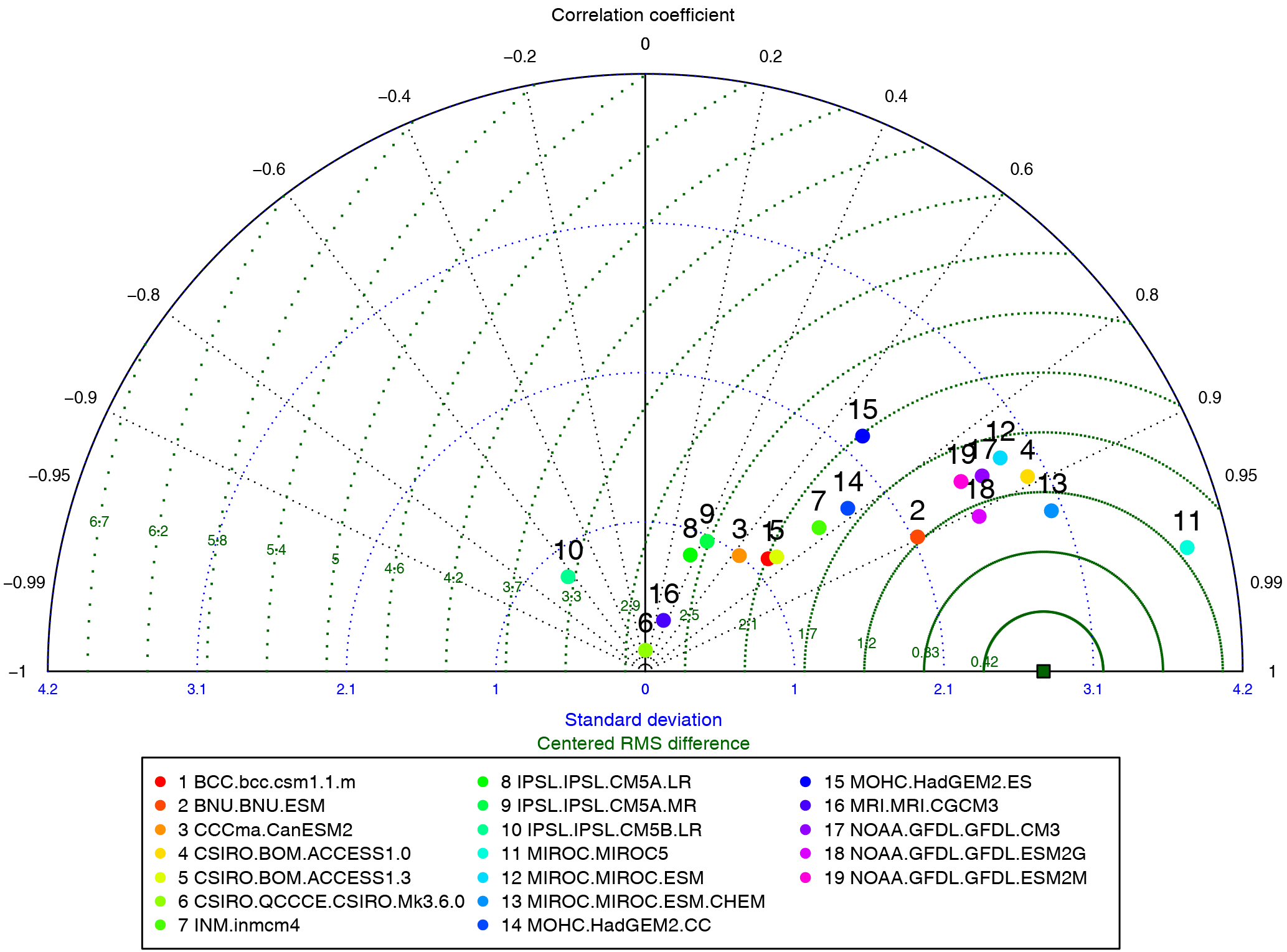
Figure A1 Taylor diagram that graphically summarises how closely the historic precipitation generated by each of the 21 CMIP5 models used in this study matches the TRMMv7 observed precipitation, over the period 2000–2005. According to that diagram, the closer a model is to the observation (dark green – squared dot in the bottom right side of graph), the better it performs.

A Taylor diagram is used to assess the relative skill of the CMIP5 models used in this study (Table A1) and estimate which of them performs better in terms of simulating historical precipitation patterns over the study area (Fig. A1). The diagram quantifies the similarity between modelled and observed precipitation in terms of the spatial pattern correlation coefficient, standard deviation and centred root-mean-square (RMS) difference (Taylor, 2001). Figure A1 graphically summarises how closely the historic precipitation generated by each of the 21 CMIP5 models used in this study matches the TRMMv7 observed precipitation, over the period 2000–2005. This plot illustrates that for the specific time period of 2000–2005, models such as CNRM-CM5, MIROC4h and MIROC5 are perceived to outperform models like IPSL-CM5B-LR or CSIRO-Mk-3-6-0 in terms of their ability to match the TRMMv7 observed precipitation well.

The spatial patterns of precipitation change between the periods 1975–2005 and 2020–2050 are shown in Fig. A2. For the summer monsoon period (JJA), the multi-model mean pattern of future projections points towards a precipitation increase for some areas of up to 1.6 mm d⁻¹ under scenario RCP4.5, whilst for other areas a decrease of up to 0.4 mm d⁻¹ is projected. As expected, under scenario RCP8.5, which corresponds to stronger radiative forcing, the precipitation increase and decrease is slightly stronger (up to +1.7 and −0.5 mm d⁻¹ respectively). For the dry period (DJF), under RCP4.5, the multi-model mean project a small decrease in precipitation for some areas (up to −0.3 mm d⁻¹), whilst it projects an increase of up to 0.11 mm d⁻¹ for other areas. Similar patterns of change are observed for DJF under RCP8.5. This means that an amplification of the annual cycle is being projected for the end of the century, with more pronounced wet and dry seasons.

Figure A3 shows the spatial patterns of temperature change between the periods 1975–2005 and 2020–2050. The projections indicate a robust signal of temperature increase in all examined periods and under both emission scenarios. The temperature increase ranges from 0.8 to 2.2 ^∘C under RCP4.5 and from 0.9 to 2.4 ^∘C under RCP8.5.

Table A1 CMIP5 model output used and data resolution.

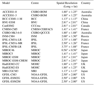
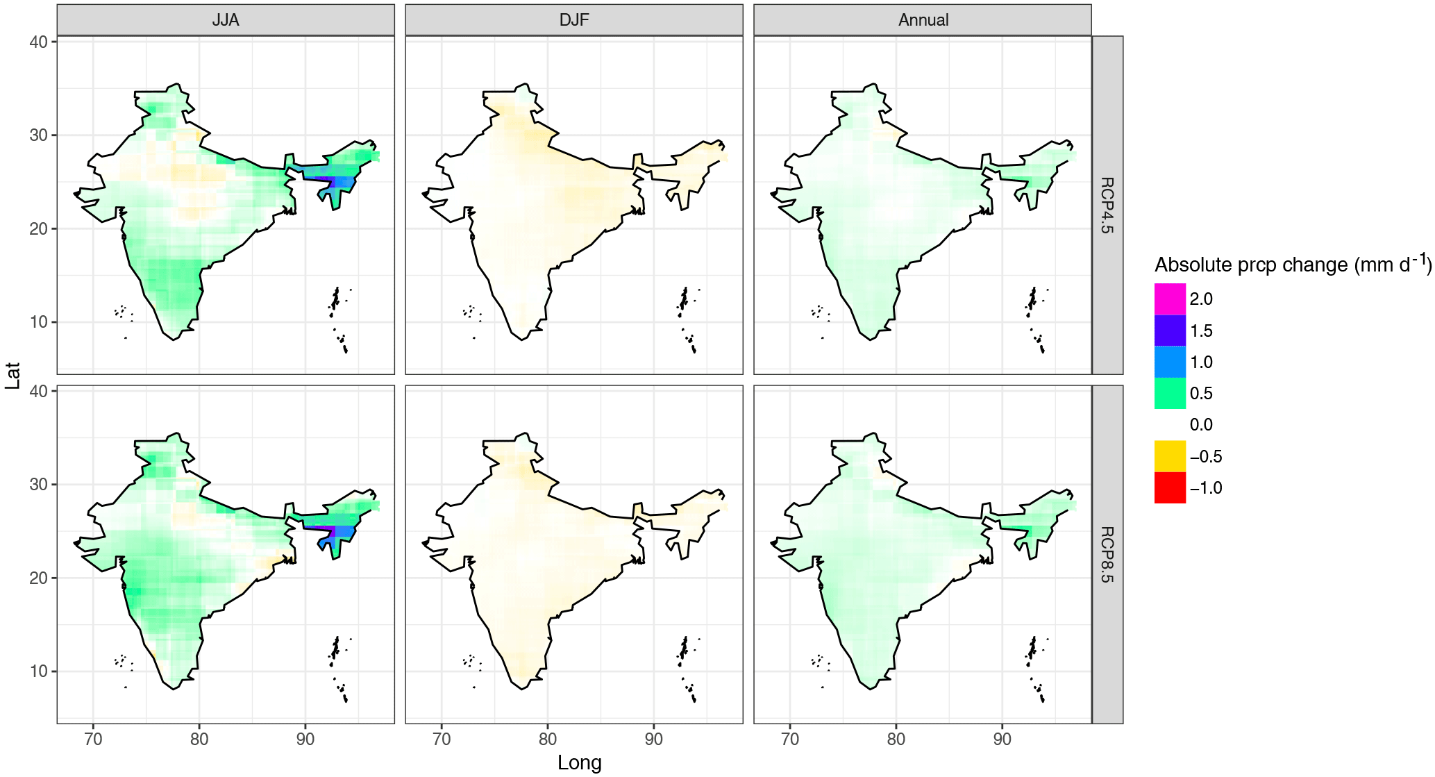
Figure A2 Absolute change (mm d⁻¹) in the multi-model mean precipitation over India between 1975–2005 and 2020–2050. Results are separated under two emission scenarios (RCP4.5 and RCP8.5) averaged over three different periods: the monsoon period (June–August, JJA), the dry winter period (December–February, DJF) and the annual period.

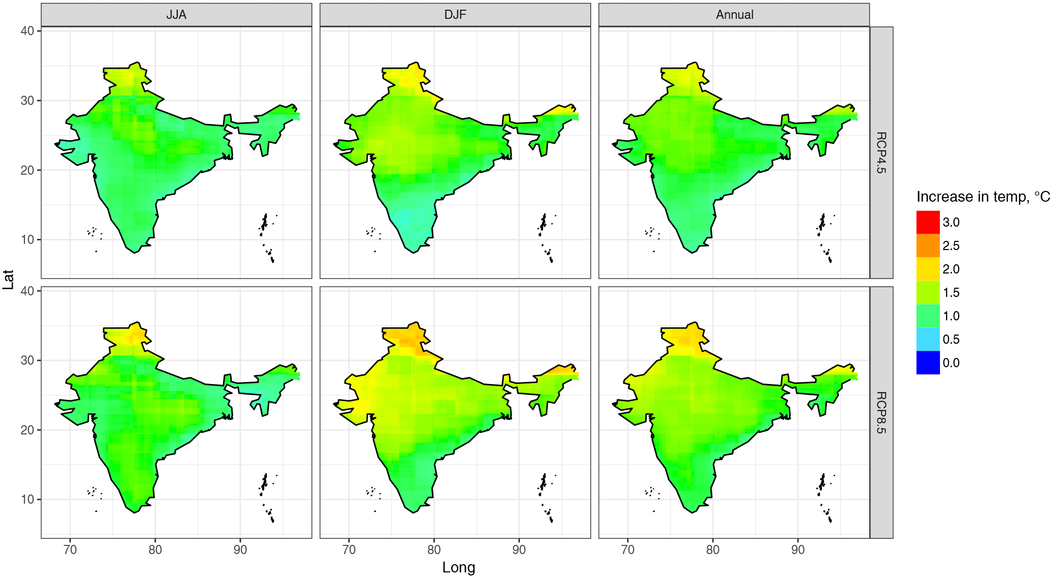
Figure A3 Absolute change (^∘C) in the multi-model mean surface air temperature over India between 1975–2005 and 2020–2050. Results are separated under two emission scenarios (RCP4.5 and RCP8.5) and three different timescales: the monsoon period (June–August, JJA), the dry winter period (December–February, DJF) and the annual period.

Appendix B: Hydrological modelling outputs

The generated streamflows (Fig. B1) reveal the impact of both climate change and land-use change in the future flows. The spread of the results is indicative of the uncertainties among different GCM forcing data. The spread is large under both emission scenarios, which suggests that the GCM precipitation spread is relatively less sensitive to the level of radiative forcing. Further, it is noticeable that the agreement in projections of low flows is stronger than that of high flows, because the future projections of extreme precipitation events have large uncertainties in the tropical regions as also mentioned in the study by Kharin et al. (2013).

Kernel density plots shown in Fig. B2 show the distributions of Q₅, Q₂₅, Q₅₀, Q₇₅ and Q₉₅ (i.e. flows exceeded 5, 25, 50, 75 and 95 % of time respectively) among different GCMs, when only climate change is taken into account (Q_cl) and when both land-use and climate change are taken into account (Q_{cl_lu}), for the Upper Ganges basin. The large variations in flows highlight the large spread among GCM outputs used to force JULES. It is evident that the differences between the two RCPs are greater than the differences between Q_cl and Q_{cl_lu} of the same RCP. As illustrated by the densities shown in Fig. B2, the agreement in projections of low flows (Q₇₅, Q₉₅) is stronger than that of high flows (Q₅, Q₂₅), as previously discussed.

The sensitivity tests we performed by running JULES under the assumption that the study area is 100 % covered by a single land-cover type are indicative of the model's sensitivity to land use. Figure B3 shows that the highest flows are generated under 100 % water or urban coverage, as would be expected due to reduced infiltration and increased discharge, whilst vegetation coverage and in particular forest and crops generate lower flows (due to higher infiltration, canopy interception and evapotranspiration rates).

The magnitude of increase in the future projections of streamflows might appear unrealistic, and this is partly attributed to the downscaling method used that increased precipitation extremes and partly to the uncertainties in GCM outputs. The mean climatic CFs were calculated from the mean monthly climatologies over 6-year time slices. However, given the large variability in precipitation on daily timescales compared to the mean monthly climatology, by scaling the high extremes of precipitation according to the CF, it is inevitable that in some cases precipitation is highly exaggerated in the future projections. In such a large catchment inflated precipitation extremes would be directly translated by JULES into unreasonably high runoff values.

In terms of evapotranspiration fluxes (Fig. 12), the multi-model mean future projections under RCP4.5 point towards increased evapotranspiration for the spring months March and April and decreased evapotranspiration over the summer period (June–September). Under RCP8.5, evapotranspiration follows similar patterns of change, although in August the projection points towards increased evapotranspiration compared to historic values. In all cases, it is evident that, in the near-term-future projections, the inter-model uncertainty is higher than the scenario uncertainty. This is also shown in Fig. B4, which displays monthly percentage changes in evapotranspiration between the historic (2000–2005) and future period (2030–2035), spatially averaged in the Upper Ganges basin. The spread of results derived by JULES forced with different GCM outputs is large under both RCPs but the multi-model mean changes are never higher than 20 %.

On the other hand, the multi-model mean future projections of soil moisture under the same scenario (Fig. 13) show a decrease in soil moisture from April to September. Interestingly, the changes in soil moisture relative to the historic period are smaller under RCP8.5 compared to RCP4.5. The overall agreement between historic and both future scenarios seems to be better in the soil moisture results compared to the evapotranspiration results (see also the spread of results in Figs. B4–B5). Figure B5 displays monthly percentage changes in soil moisture between the historic (2000–2005) and future projections period (2030–2035), spatially averaged in the Upper Ganges basin. It is shown that the spread of results is larger under RCP4.5 compared to RCP8.5. This could be explained by the stronger forcing of the RCP8.5, which leads the GCMs to produce more similar results. In all cases the multi-model mean changes between historic and future projections in soil moisture are never higher than approximately 20 %.

It is likely that the delta-change approach followed in this study contributed to the exaggeration of the highest extremes in the daily historical precipitation. This exaggeration, accumulated over days and a large basin, could produce excessive amounts of runoff. In addition, the differences between the two RCP scenarios are not large, especially for the projections of evapotranspiration and soil moisture fluxes. In the nearby-future period examined here (2030–2035), the relative importance of the RCPs is far smaller than the GCM model uncertainties. Finally, it is important to note that this study did not explicitly address future changes in irrigation practices that could have a large impact in evapotranspiration rates over the study area.

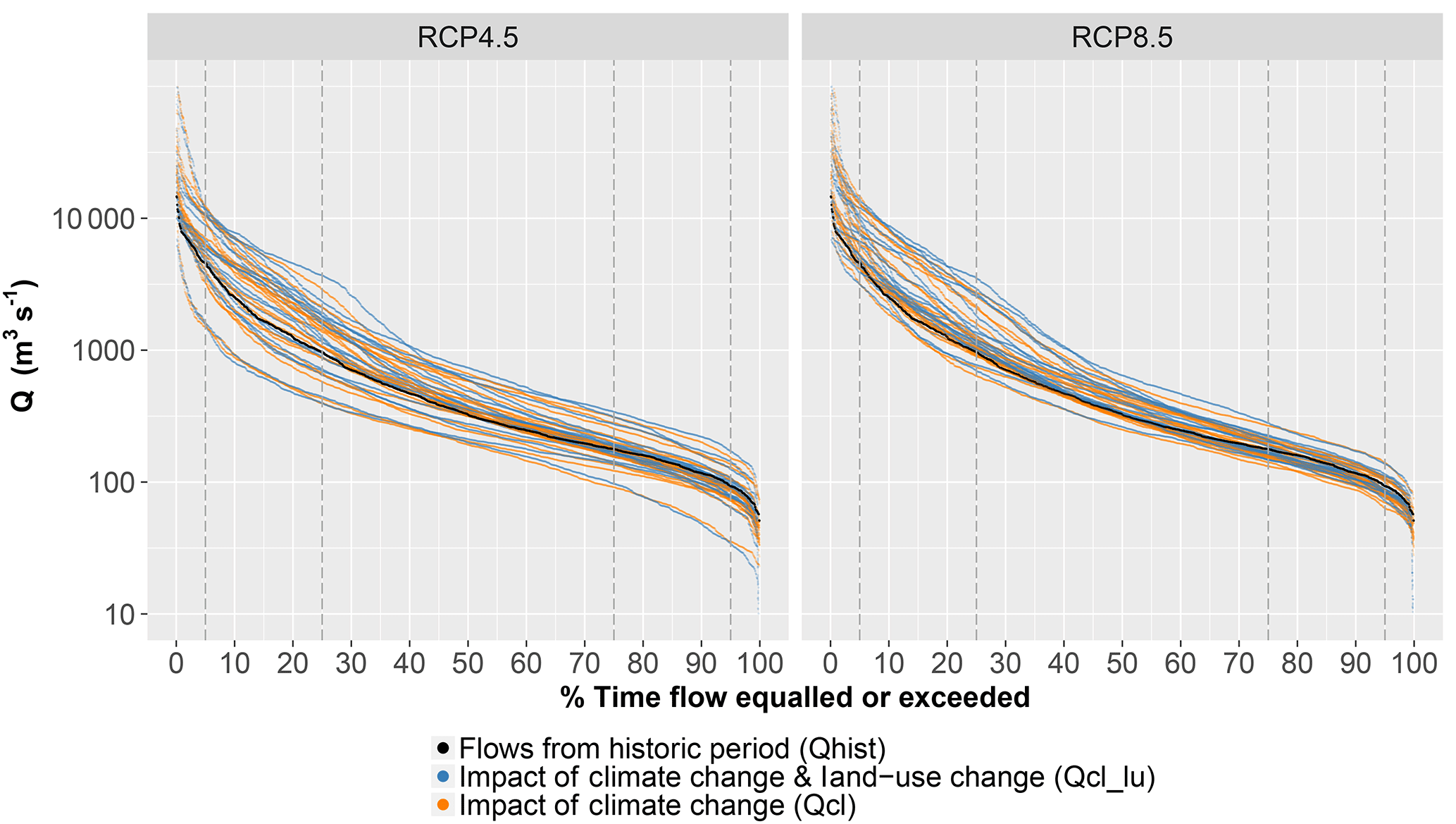
Figure B1 Flow duration curves of the streamflows simulated by JULES for the Upper Ganges basin, when forced by CMIP5 model outputs. Orange: only climate change is taken into account (Q_cl); simulation period 2030–2035; each line represents JULES outputs based on different CMIP5 model forcing. Blue: both climate change and land-use change are taken into account (Q_{cl_lu}); simulation period 2030–2035; each line represents JULES outputs based on different CMIP5 model forcing. Black: historical period (Q_hist); simulation period 2000–2005.

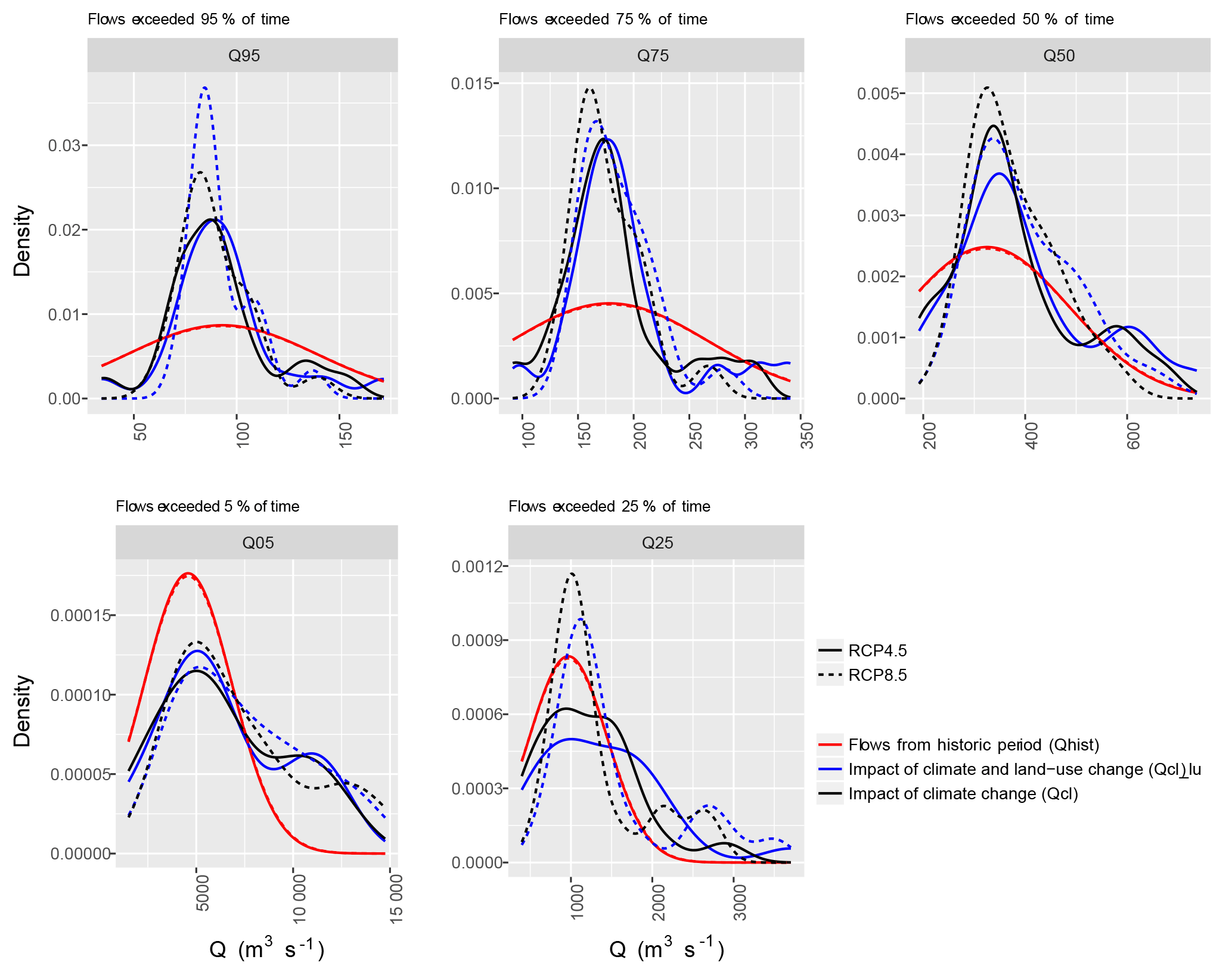
Figure B2 Kernel density plots showing distribution of Q₅, Q₂₅, Q₅₀, Q₇₅ and Q₉₅ (i.e. flows exceeded 5, 25, 50, 75 and 95 % of time respectively) among different GCMs, for the Upper Ganges basin, under both emission scenarios. Black: only climate change is taken into account (Q_cl); simulation period 2030–2035. Blue: both climate change and land-use change are taken into account (Q_{cl_lu}); simulation period 2030–2035. Red: historical period (Q_hist); simulation period 2000–2005.

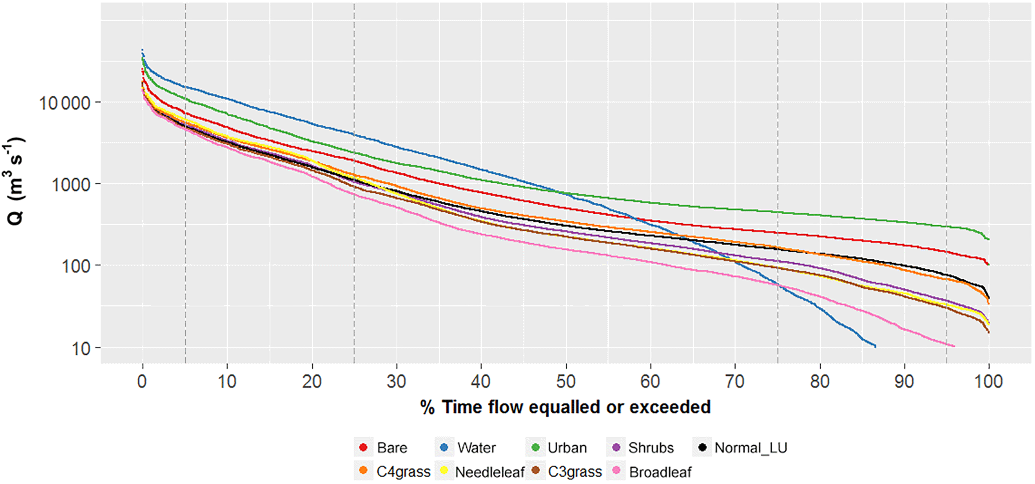
Figure B3 Flow duration curves of the streamflows simulated by JULES for the Upper Ganges basin, at Kanpur barrage, under the assumption that the study area was 100 % covered by a particular land-cover type. For reference, the results of the run with the 2010 land-cover map are also plotted (normal_LU).

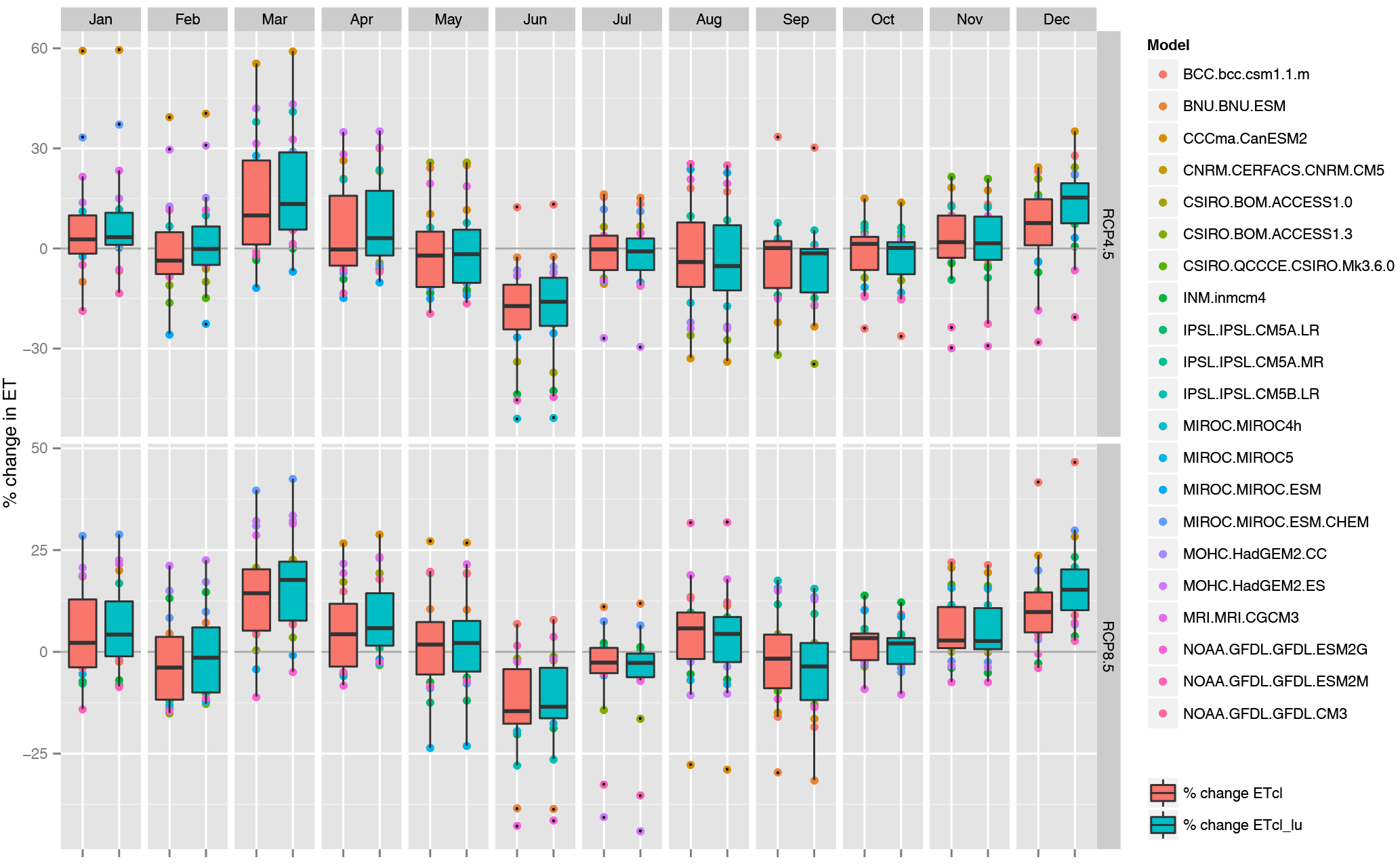
Figure B4 Percentage changes in evapotranspiration (ET) fluxes between the historical simulation period 2000–2005 and the future projection simulation period 2030–2035 for the Upper Ganges basin and for each of the emission scenarios (RCP4.5 and RCP8.5). Pink colour corresponds to the scenarios where only climate change is taken into account. Blue colour corresponds to the scenarios where both climate change and land-use change are taken into account.

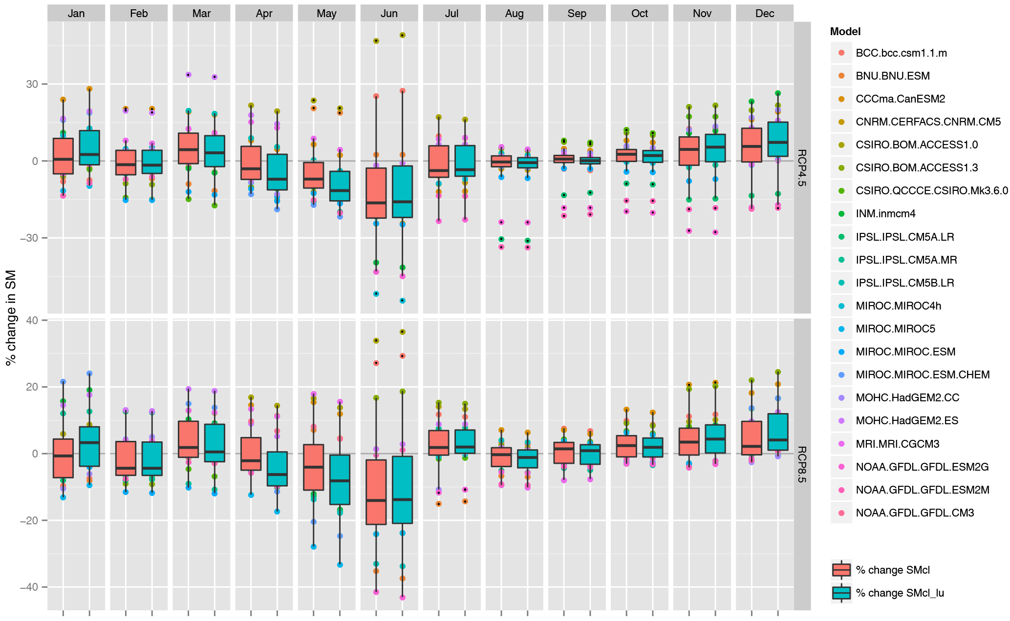
Figure B5 Percentage changes in soil moisture fluxes between the historical simulation period 2000–2005 and the future projection simulation period 2030–2035 for the Upper Ganges basin and for each of the emission scenarios (RCP4.5 and RCP8.5). Pink colour corresponds to the scenarios where only climate change is taken into account. Blue colour corresponds to the scenarios where both climate change and land-use change are taken into account.