Developing Intensity-Duration-Frequency (IDF) curves using sub-daily gridded and in situ datasets: characterising precipitation extremes in a drying climate

Traditionally, Intensity-Duration-Frequency (IDF) curves are based on rain gauge data under the assumption of stationarity. However, only limited long time series of sub-daily precipitation data are available worldwide, making it difficult to accurately estimate precipitation intensity for different durations and return periods, while climate change is challenging stationarity. This study aims to better understand how the stationary assumption and data length of hourly precipitation data influence the annual maximum intensities of precipitation events in continental Chile, a region with varying climate and topography that has been affected by an unprecedented drought since 2010. Five hourly gridded precipitation datasets (IMERGv06B, IMERGv07B, ERA5, ERA5-Land, CMORPH-CDR) and 161 quality-checked rain gauges are used to compute annual maximum intensities (I_max, mm h⁻¹) using the stationary and non-stationary Gumbel distribution for six return periods (2–100 years) and 11 durations (1–72 h). Bias-correction factors are applied to match the gridded I_max values with the in situ ones, and the modified Mann–Kendall test is used to assess the trends in I_max. Annual maximum intensities are calculated for the 20 year period (2001–2021) for all products, while an additional 40 year period (1981–2021) is used for ERA5 and ERA5-Land to assess the impact of data length. Our results revealed significant decreasing trends across Chile for CMORPH-CDR, decreasing trends in Central-Southern Chile (32–43° S) for ERA5 and ERA5-Land, and isolated, divergent trends for IMERGv06B and IMERGv07B. In addition, our results show that the annual maximum intensities derived from stationary and non-stationary models (I_max) reached its highest values in central and southern Chile, for all durations and return periods, in contrast to the spatial pattern of mean annual precipitation, which increases steadily towards the south. For durations of 24 h or more, the highest intensities are primarily found in the Andes, particularly between the Maule and Araucanía region (35–40° S). While the I_max values were similar for IMERGv07B, ERA5 and ERA5-Land, they were much higher for IMERGv06B and CMORPH-CDR. The difference between stationary and non-stationary I_max values ranges from 0 to 5 mm h⁻¹ and become smaller for durations greater than 8 h. Despite the differences observed in the Gumbel parameters for ERA5 and ERA5-Land when using 20- and 40 year records, the resulting I_max values showed differences with median values below 1 mm h⁻¹. The I_max values are available on a public and user-friendly web platform (https://curvasIDF.cl/, last access: 18 December 2025).

1 Introduction

Accurately estimating extreme precipitation (P) events is crucial for various engineering, hydrology, and climate science applications. One of the essential tools used by engineers worldwide for quantifying extreme precipitation events are the Intensity-Duration-Frequency (IDF) curves (Sherman, 1931; Bernard, 1932; Haruna et al., 2023), which represent statistical relationships between intensity (precipitation depth divided by duration), duration (e.g. 30 min, 1, 24 h) and frequency of occurrence of extreme precipitation events. IDF curves are constructed by fitting a theoretical probability distribution function (pdf) to samples of annual maximum (AM) or peak-over-threshold (POT) precipitation data (Yan et al., 2021). These curves are central to urban infrastructure design, stormwater management and flood risk assessment.

Notwithstanding the assumption of stationarity in precipitation extremes, i.e. a time-invariant probability distribution, has been widely debated in recent decades (Milly et al., 2008; Montanari and Koutsoyiannis, 2014; Koutsoyiannis and Montanari, 2015; Serinaldi and Kilsby, 2015; Serinaldi, 2015; Milly et al., 2015; Beven, 2016), IDF curves are still predominantly developed under this assumption for most engineering and practical applications. This reliance on stationarity can lead to infrastructure failures during extreme events in a changing climate (Cheng and Aghakouchak, 2014; Mohan et al., 2023). While stationarity simplifies the construction of IDF curves, it may not adequately capture climate change impacts or long-term variability in precipitation intensities.

On the other hand, non-stationary IDF curves consider the time-dependent nature of distribution parameters and can capture existing trends in precipitation intensity (e.g. Agilan and Umamahesh, 2018; Ouarda et al., 2019; Yan et al., 2021; Silva et al., 2021; Vinnarasi and Dhanya, 2022; Schlef et al., 2023). Several approaches have been developed in the last decades for computing non-stationary intensity-duration-frequency curves, to face changing precipitation patterns (e.g. Cheng and Aghakouchak, 2014; Agilan and Umamahesh, 2016, 2017, 2018; Salas et al., 2018; Ouarda et al., 2019; Nwaogazie and Sam, 2020; Yan et al., 2021; Schlef et al., 2023). Among them, Schlef et al. (2023) provides a comprehensive review of IDF curves under non-stationary conditions, including global precipitation trends, estimation methods, regionalization challenges, and uncertainty in design values.

While the aforementioned methods rely on stationary or non-stationary statistical models to summarise historical data, Koutsoyiannis et al. (2024) introduced a stochastic framework that models precipitation as a random process, and provides a probabilistic and theoretically grounded approach to estimating the relationships between intensity and duration across time scales (durations) and return periods. This method accounts for the inherent variability and uncertainty of precipitation events without relying on stationary assumptions, and potentially provides more robust estimates under changing climate conditions (Iliopoulou et al., 2024).

Regarding the data sources used to build IDF curves, traditionally they have been derived from point measurements obtained from rain gauges installed on the ground (e.g. Chow et al., 1988; Koutsoyiannis et al., 1998; Sivapalan and Blöschl, 1998; Watkins et al., 2005). However, point-based precipitation data obtained from rain gauges, while valuable, present limitations in capturing the true spatio-temporal variability of precipitation patterns, due to the relocation of stations, the use of different types of rain gauges, among others (Wood et al., 2000; Habib et al., 2001; Villarini et al., 2008; Gianotti et al., 2013; Pollock et al., 2018; Morbidelli et al., 2020; Fadhel and Saleh, 2021). In particular, worldwide there is a limited availability of long time series of sub-daily rainfall data. As a result, the true value of individual annual maximum rainfall depths might be underestimated up to 50 % for short durations, i.e. when the event duration is similar or lower than one day. The use of uncorrected series of annual maxima can lead to underestimations of ∼10 % in the resulting IDF curves (Morbidelli et al., 2017, 2020).

To overcome these limitations, gridded precipitation products have emerged in recent decades, providing spatially continuous and temporally homogeneous datasets that offer a more comprehensive representation of precipitation dynamics (Funk et al., 2015; Huffman et al., 2017; Xie et al., 2017; Beck et al., 2019a, b, 2022; Baez-Villanueva et al., 2020; Nguyen et al., 2020; Muñoz-Sabater et al., 2021; Sadeghi et al., 2021). These gridded precipitation products have opened up new opportunities to improve the accuracy and spatial representation of IDF curves, especially in regions with complex topography and climatic variability (Endreny and Imbeah, 2009; Marra et al., 2017; Ombadi et al., 2018; Faridzad et al., 2018; Sun et al., 2019; Noor et al., 2021; Venkatesh et al., 2022). Their improved resolution and coverage make them valuable tools for various scientific and engineering applications, while also advancing our understanding of extreme precipitation events. However, estimates of gridded precipitation products are not directly comparable to rain gauge measurements, because gridded estimates represent area-averaged values, which can smooth out variability.

Notwithstanding the previous limitation, in the last decades these precipitation products have been extensively evaluated against in situ measurements (e.g. Aghakouchak et al., 2011; Ward et al., 2011; Chen et al., 2013; Duan et al., 2016; O et al., 2017; Zambrano-Bigiarini et al., 2017; Baez-Villanueva et al., 2018; Beck et al., 2019a) and used for hydrological purposes (Casse et al., 2015; Bisselink et al., 2016; Maggioni and Massari, 2018; Baez-Villanueva et al., 2020, 2021; Fernandez-Palomino et al., 2022; Aguayo et al., 2024). However, only a few studies have focused on the development of IDF curves from publicly available gridded precipitation datasets for different regions (Endreny and Imbeah, 2009; Marra et al., 2017; Faridzad et al., 2018; Ombadi et al., 2018; Sun et al., 2019; Courty et al., 2019; Noor et al., 2021; Venkatesh et al., 2022). These studies highlight the potential of these products as an alternative to in situ rainfall data for developing IDF curves, but also describe some challenges. Ombadi et al. (2018) mention that errors in IDF curves derived from gridded datasets are related to the ability of the original product to reproduce the maximum rainfall intensities and to uncertainties derived from the short length of the data records, highlighting the necessity of bias adjustment from local rain gauges to provide accurate quantile estimates. Sun et al. (2019) emphasise the importance of sub-daily rainfall records to obtain reliable IDF curves.

In this study, we aim to address the previously mentioned challenges by deriving IDF curves from five state-of-the-art hourly-gridded precipitation datasets and 161 hourly rain gauges. In particular, we address the following research questions:

1. What is the spatial distribution of the stationary annual maximum precipitation intensities for different durations?

2. Are there any significant trends in the stationary annual maximum precipitation intensities that justify using non-stationary IDF curves?

3. Is the difference between stationary and non-stationary IDF curves significant enough to justify using a non-stationary analysis?

4. What is the impact of the typical data length of precipitation products used for estimating stationary and non-stationary IDF curves?

In other words, this study aims to better understand how the spatial distribution, temporal trends and data length of hourly precipitation data influence the use of stationary vs. non-stationary IDF curves in a study area with diverse climate zones and topography. Additionally, it would provide practical guidance for hydrological and engineering applications that require a reliable quantification of extreme precipitation events.

This article is organised as follows: Sect. 2 describes the study area and datasets, while Sect. 3 describes the methodology used to develop stationary and non-stationary IDF curves. Numerical and graphical results, along with an in-depth discussion in the light of the wider literature, are described in Sect. 4. Concluding remarks are summarised in Sect. 5, followed by practical recommendations that should be considered by decision-makers.

2 Study area and datasets

2.1 Study area

Our study area is continental Chile, with more than 4000 km of latitudinal extension (17.5–56.5° S), from the Pacific Ocean in the west (∼76° W) to the Andes mountains in the east (∼66° W). It covers an area of ∼756 626 km², with elevations ranging from sea level to 6893 $\mathrm{m}\mathrm{a}.\mathrm{s}.\mathrm{l}.$, encompassing four distinctive geomorphological units: coastal plains, coastal mountain range, intermediate depression, and the Andes mountain range. This area exhibits exceptional climatic variability (11 different climates), ranging from hot and dry deserts in the north to polar and tundra climates in the south (Fig. 1).

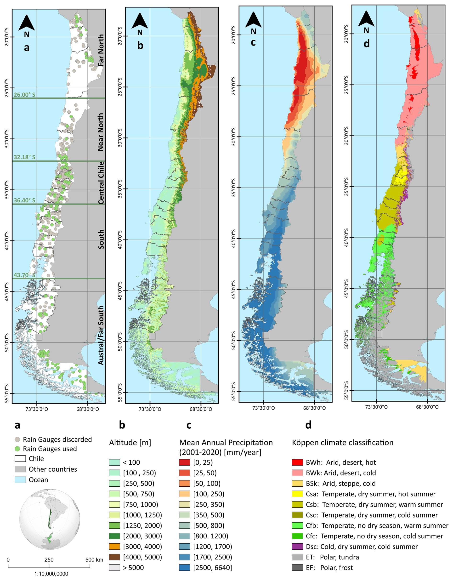
Figure 1 Study area. From left to right: (a) rain gauges and macro-climatic zones; (b) digital elevation model (Jarvis et al., 2008); (c) mean annual precipitation (ERA5-Land; Muñoz-Sabater et al., 2021) (d) Köppen–Geiger climate classes (Beck et al., 2023).

To better describe the spatial patterns of extreme precipitation, we divided our study area into five macro-climatic zones, slightly adapted from Zambrano-Bigiarini et al. (2017): Far North (17.5–26.0° S); Near North (26.0–32.2° S); Central Chile (32.2–36.2° S), South (36.4–43.7° S) and Austral/Far South (43.7–56.5° S). Figure 1 shows the macro-climatic zones, elevations (Jarvis et al., 2008), mean annual precipitation (Muñoz-Sabater et al., 2021), and the Köppen–Geiger climate classification (Beck et al., 2023) for our study area.

2.2 Datasets

2.2.1 Rain gauges

The General Directorate of Water (DGA), the Meteorological Directorate of Chile (DMC), the Agrometeorological Network of the Agricultural Research Institute (Agromet) and the Center for Advanced Studies in Arid Zones (CEAZA) have more than 600 rain gauges with hourly time series of observed precipitation in Chile. All these raw hourly records (GMT-4) from 2000 to 2021 are publicly available in the Vismet web platform (https://vismet.cr2.cl/, last access: 1 December 2024) of the Center of Climate and Resilience Research (CR2).

After an exploratory analysis and basic quality control, we discarded 406 Agromet stations due to the existence of some anomalously large precipitation values. For the remaining 194 stations, we analysed the amount of hourly data effectively available for several 5 year temporal periods (see Supplement S1 in Soto-Escobar et al., 2025), which led to the selection of 161 rain gauges with more than 80 % hourly data between 1 January 2013–31 December 2017. Figure 1a shows the location of the 161 selected rain gauges, which are described in Table S1 in the Supplement S1 at https://doi.org/10.5281/zenodo.16956066 (Soto-Escobar et al., 2025).

2.2.2 Gridded precipitation datasets

In this study, we initially analysed six gridded precipitation datasets. However, our analysis and results are only presented for five of them, listed in Table 1. The sixth dataset, Precipitation Estimation from Remotely Sensed Information Using Artificial Neural Networks–Dynamic Infrared Rain Rate (PDIR-Now, Nguyen et al., 2020), was ultimately not included in this manuscript (see details in the Supplement S2; Soto-Escobar et al., 2025). The five gridded precipitation datasets finally used for this study are briefly described in the following sections.

Huffman et al. (2015, 2017)Huffman et al. (2023, 2024)Hersbach et al. (2018, 2020)Muñoz-Sabater (2019); Muñoz-Sabater et al. (2021)Xie et al. (2017)Xie et al. (2018)

Table 1 Gridded P datasets used in this study.

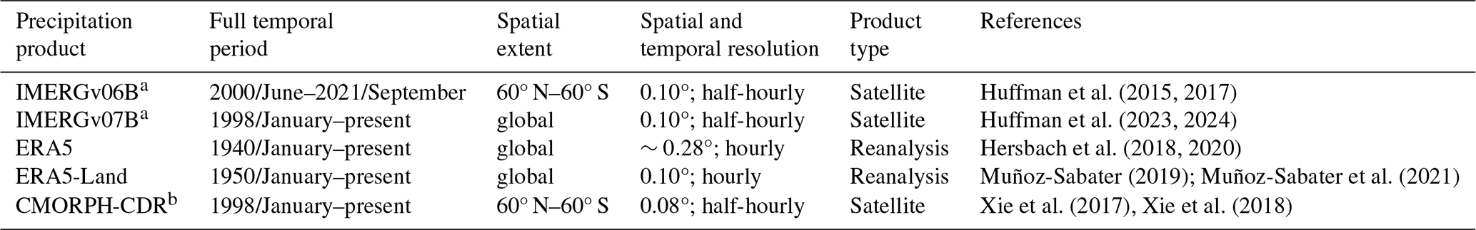
^a Global Precipitation Climatology Centre (GPCC) monthly precipitation data for 1891–present is used for corrections. ^b CPC Unified Daily Gauge Analysis (over land) and the Global Precipitation Climatology Project (GPCP) pentad dataset (over oceans) are used for corrections.

IMERG V06B Final Run

The Integrated Multi-satellitE Retrievals for GPM (IMERG) is a precipitation product developed by NASA as a part of the Global Precipitation Measurement (GPM) mission (Huffman et al., 2015). It integrates data from passive microwave and infrared sources to create an instantaneous precipitation estimate at a 30 min, 0.1° resolution globally from 2000 to the present, allowing it to capture a wide range of precipitation events, from light rain to heavy storms (Huffman et al., 2017). To reduce biases inherent to satellite-only retrievals, monthly satellite precipitation totals are first aligned with the GPCC Monitoring Product, and then the high-resolution satellite estimates are rescaled accordingly.

We used the retrospective IMERG V06B Final Run dataset, hereafter IMERGv06B, which provides precipitation intensities (mm h⁻¹$/\mathrm{10}$) every 30 min, from 00:00 to 23:59 UTC+00 and from 1 June 2000 to 30 September 2021. To work with complete years only, we selected data from 1 January 2001 to 31 December 2020 (i.e. 20 years of data and 350 640 half-hourly files). We downloaded the half-hourly GeoTiff files from NASA (http://pmm.nasa.gov/data-access/, last access: January 2019–December 2022) using the WGS84 geodetic geographic coordinate system. Finally, we corrected the IMERG gridded geolocation error of 0.1° (one-pixel) shift westward for all grid boxes, described in the Appendix 1 of Huffman et al. (2024).

IMERG V07B Final Run

The Integrated Multi-satellitE Retrievals for GPM (IMERG) dataset provides global precipitation estimates at 0.1° spatial and half-hourly temporal resolution. The latest version, IMERG V07 (released in 2023), incorporates several major upgrades over V06B (Tan et al., 2022; Huffman et al., 2024). These include enhanced calibration of passive microwave observations, updated CORRA and GPROF retrieval algorithms, refined infrared (IR) estimates with improved quality control, and better detection of precipitation phase near freezing temperatures. Additional improvements involve expanded coverage over frozen surfaces, correction of the spatial offset present in earlier versions, and increased consistency across the Early, Late, and Final runs. IMERG V07 also extends the data record back to 1998 using GridSat-B1 observations, providing more than 20 years of uniformly reprocessed precipitation estimates from the TRMM and GPM eras. Collectively, these updates make IMERG V07 a more accurate, consistent, and globally applicable dataset than its predecessors.

Similarly to IMERGv06B, we used the retrospective IMERG V07B Final Run dataset, hereafter IMERGv07B, which provides precipitation intensities (mm h⁻¹$/\mathrm{10}$) every 30 min, from 00:00 to 23:59 UTC+00 and from January 1998 to present. Due to data availability during our data processing, we downloaded data from 1 January 2001 to 31 December 2021 (i.e. 21 years of data and 368 160 half-hourly files). We downloaded the half-hourly GeoTiff files from NASA (https://arthurhouhttps.pps.eosdis.nasa.gov/gpmdata/, last access: December 2023) using the WGS84 geodetic geographic coordinate system.

ERA5

The fifth Generation of the European Centre for Medium-Range Weather Forecasts (ECMWF) Reanalysis (ERA5) supersede the previous ERA-Interim used from 2006 to 2019, and provides a comprehensive and high-quality dataset of various atmospheric variables, including precipitation (Hersbach et al., 2020). It combines observations and model simulations, assimilating a vast amount of data sources to produce hourly precipitation estimates on a regular grid with a spatial resolution of 0.25°, which allows for detailed analyses of precipitation dynamics at regional and global scales (Hersbach et al., 2020). Since 2009, ERA5 assimilates ground-based radar-gauge composite observations over certain regions (notably the contiguous United States), but it is not systematically bias-corrected globally using a dense rain-gauge network. We downloaded hourly data from the Copernicus Climate Data Store (Hersbach et al., 2018).

ERA5-Land

ERA5-Land is a high-resolution reanalysis dataset that provides land-focused variables from the ERA5 system at 0.1° (∼9 km) spatial and hourly temporal resolution (Muñoz-Sabater et al., 2021). It is specifically designed to represent the spatio-temporal dynamics of the water and energy cycles over land, including variables such as soil temperature, soil moisture, snow cover, and vegetation properties, while ERA5 also includes ocean components. Precipitation in ERA5-Land is obtained by linearly interpolating ERA5 forcing data onto a finer triangular mesh, without applying bias correction to the original ERA5 fields. Compared to ERA5, the input atmospheric variables (like temperature, humidity, and pressure) used for ERA5-Land are corrected for altitude differences between the ERA5 grid and the ERA5-Land grid to account for elevation effects, which improves the representation of land surface processes (Muñoz-Sabater et al., 2021). We downloaded hourly ERA5-Land data from the Copernicus Climate Data Store (Muñoz-Sabater, 2019).

Although ERA5 and ERA5-Land share the same underlying reanalysis, their differences in spatial resolution and land-surface representation might have meaningful implications for characterising sub-daily extreme precipitation. Including both datasets allows us to assess whether the finer resolution and enhanced land-surface processes in ERA5-Land improve the estimation of IDF curves compared to ERA5, providing insights into the influence of spatial detail on extreme precipitation metrics. This comparison is particularly relevant for researchers and practitioners across hydrology, climatology, and water resources, as it highlights potential trade-offs between computational cost, data volume, and the added value of higher-resolution products.

CMORPH-CDR

The National Oceanic and Atmospheric Administration (NOAA) uses the Climate Prediction Center (CPC) morphing technique (CMORPH; Joyce et al., 2004) to create near-real-time and high-resolution satellite precipitation estimates at the global scale. CMORPH estimates are obtained exclusively from passive microwave observations from low-orbiting satellites (PMW) and then transported in space using infrared data from geostationary satellites during periods when no direct PMW data are available (Joyce et al., 2004).

Unlike the original CMORPH, which does not include any bias correction, the Climate Data Record (CDR) version of CMORPH (Xie et al., 2017, 2018) incorporates the CPC Unified Daily Gauge Analysis (over land) and the Global Precipitation Climatology Project (GPCP) pentad dataset (over oceans) to bias correct the raw integrated CMORPH satellite precipitation estimates. These corrections ensure improved temporal consistency and spatial homogeneity, essential for long-term climate studies (Bates and Barkstrom, 2006).

CMORPH-CDR is a quasi-global dataset (60° N–60° S) with a spatial resolution of 8 km and half-hourly temporal frequency, starting from 1 January 1998 (Xie et al., 2017, 2018). In this work, we used CMORPH-CDR version 1, hereafter CMORPH-CDR, which is produced manually once a month with a latency of 3–4 months (Xie et al., 2018). We downloaded half-hourly NetCDF files from NOAA (https://www.ncei.noaa.gov/products/climate-data-records/precipitation-cmorph, last access: June 2022) using the WGS84 geodetic geographic coordinate system.

3 Methodology

After downloading the original datasets, the half-hourly precipitation products (IMERGv06B, IMERGv07B and CMORPH-CDR) were aggregated into hourly intervals to ensure consistency in the temporal resolution used for the subsequent analyses. As a basic first checking, all the products were able to reproduce the spatial distribution of annual mean precipitation when compared with the Chilean CR2METv2.5 gridded precipitation product (Boisier, 2023). All the spatio-temporal analyses were carried out using the terra (Hijmans, 2025) and hydroRTS (Zambrano-Bigiarini and Bernal Vallejos, 2023) R packages (R Core Team, 2024).

Figure 2 illustrates the procedure used to address the research questions outlined in Sect. 1: (i) estimation of annual maximum intensities for different durations d using stationary and non-stationary statistical models, for each one of the 161 in situ rain gauges, and for the five gridded precipitation datasets described in Sect. 2.2; (ii) computation of bias-correction factors for each gridded dataset, to match the annual maximum intensities observed at each rain gauge; (iii) assessment of the temporal evolution of the bias-corrected annual maximum intensities using the modified Mann–Kendall trend tests; (iv) estimation of annual maximum intensities for different durations and return periods T and each one of the bias-corrected gridded datasets, using both the stationary and non-stationary Gumbel probability distribution. Finally, for ERA5 and ERA5-Land, we additionally estimated annual maximum intensities using 40 (1981–2021) and 20 (2001–2021) years of hourly precipitation data, to test the impact of the data length used in the computation of annual maximum intensities, for both the stationary and non-stationary approaches.

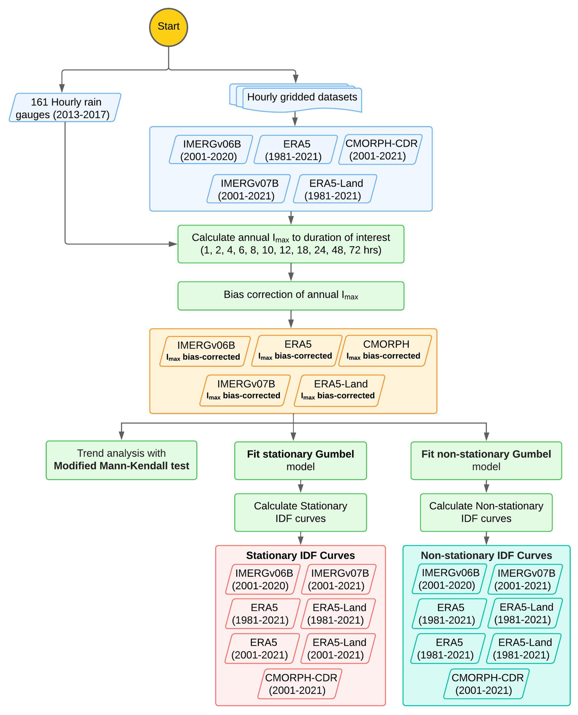
Figure 2 Flowchart summarising the methodology used to compute I_max values from both the stationary and non-stationary models for each gridded precipitation dataset.

3.1 Annual maximum intensities (I_max)

In this study, IDF curves are developed by fitting stationary and non-stationary statistical models to samples of annual maximum precipitation data. The annual maximum precipitation intensities corresponding to various durations d, as estimated by these models, are hereafter denoted as I_max (mm h⁻¹).

For the 161 selected rain gauges and for the five gridded precipitation datasets described in Sect. 2.2, we computed I_max for durations d of 1, 2, 4, 6, 8, 10, 12, 18, 24, 48, and 72 h. In contrast to the widely used fixed time windows (e.g. for a duration of 2 h, intensities are computed from 00:00 to 02:00 UTC, 02:00 to 04:00 UTC, …), we used moving time windows (Soto and Mier, 2013a, b; Moraga et al., 2015), where each selected duration becomes the length of a moving time window used to sum the hourly precipitation data along the selected duration. For example, when computing the maximum precipitation intensity for a duration of 2 h, the hourly precipitation data are aggregated from 00:00 to 02:00 UTC, from 01:00 to 03:00 UTC, from 02:00 to 04:00 UTC, …, and then the corresponding annual maximum is computed for every 2 h moving window in any given year. The adoption of a moving window instead of a fixed window is expected to avoid the omission of the highest intensities in each duration (Haruna et al., 2023).

3.2 Bias correction of I_max

Several studies have evaluated satellite-based precipitation products by comparing them with in situ measurements (e.g. Beck et al., 2020; Baez-Villanueva et al., 2018; Ombadi et al., 2018; Zambrano-Bigiarini et al., 2017), with a consensus that both random and systematic errors are present in any gridded precipitation data. Following Ombadi et al. (2018), we first computed bias-correction factors for each gridded precipitation dataset to achieve a good agreement between the I_max observed at each rain gauge and the I_max obtained at the corresponding grid cell of each gridded dataset. The procedure can be summarised as follows:

1. Computation of I_max,d. For each one of the 161 selected rain gauges, and for durations d of 1, 2, 4, 6, 8, 10, 12, 18, 24, 48, and 72 h, we used the moving time windows described in Sect. 3.1 to compute: (i) the I_max in each rain gauge RG ($I_{{\text{max}}_{d,\text{RG, year}}}$), and (ii) the I_max for each gridded precipitation product PP at the grid cell where a rain gauge RG is located ($I_{{\text{max}}_{d,\text{PP, year}}}$), where the year index represent the year under analysis.

2. Computation of S_{d,RG, year}. For each duration d and grid cell where a rain gauge RG is located, we computed an annual bias correction factor S_{d,RG, year}, where the year index represent the year under analysis, as follows (Venkatesh et al., 2022; Nguyen et al., 2020; Arias-Hidalgo et al., 2013):

   $$\begin{array}{}\text{(1)}& {\displaystyle }{\displaystyle }{S}_{d,\text{RG, year}}={\displaystyle \frac{I_{{\text{max}}_{d,\text{RG, year}}}}{I_{{\text{max}}_{d,\text{PP, year}}}}}\end{array}$$

3. Computation of ${\stackrel{\mathrm{‾}}{S}}_{d,\text{RG}}$. To correct the systematic error in each gridded precipitation dataset we computed average annual bias-correction factors (${\stackrel{\mathrm{‾}}{S}}_{d,\text{RG}}$) for each grid cell and duration d where a rain gauge RG is located as follows:

   $$\begin{array}{}\text{(2)}& {\displaystyle }{\displaystyle }{\stackrel{\mathrm{‾}}{S}}_{d,\text{RG}}=\sum _{n=\mathrm{1}}^{n\text{years}}{\displaystyle \frac{S_{d,\text{RG, year}}}{n\text{years}}}\end{array}$$

   where nyears represents the amount of years used in the analysis of each precipitation dataset.

4. Interpolation of average annual bias-correction factors (${\stackrel{\mathrm{‾}}{S}}_{d,\text{interp}}$) for each duration. To obtain bias-correction factors for the whole spatial extent of the study area and each duration d, we interpolated the average annual bias-correction factors obtained at the 161 selected rain gauges using a thin plate spline interpolation (Karger et al., 2021), as implemented in the fields R package (Nychka et al., 2021; R Core Team, 2024). This resulted in a gap-free surface of interpolated bias-correction factors ${\stackrel{\mathrm{‾}}{S}}_{d,\text{interp}}$.

5. Computation of bias-corrected gridded I_max for each duration. Finally, we computed bias-corrected annual maximum intensities for each duration d ($I_{{\text{max}}_{d,\text{BC}}}$) by multiplying the previously computed ${\stackrel{\mathrm{‾}}{S}}_{d,\text{interp}}$ surface by the annual maximum intensity of each gridded precipitation product, ($I_{{\text{max}}_{d,\text{PP}}}$), as follows:

   $$\begin{array}{}\text{(3)}& {\displaystyle }{\displaystyle }{I}_{{\text{max}}_{d,\text{BC}}}=I_{{\text{max}}_{d,\text{PP}}}\cdot {\stackrel{\mathrm{‾}}{S}}_{d,\text{interp}}\end{array}$$

3.3 Trends in I_max

Following Cheng et al. (2014) and Cheng and Aghakouchak (2014), we investigated whether using non-stationary IDF curves is justified for our study area or not. We used the non-parametric modified Mann–Kendall test (Hamed and Rao, 1998) to identify the existence of monotonic upward or downward trends over time in the bias-corrected annual maximum intensities ($I_{{\text{max}}_{d,\text{BC}}}$) (Cheng et al., 2014). The modified Mann–Kendall trend test adjusts for autocorrelation to prevent false trends. It detrends the time series, calculates the effective sample size using significant serial correlations, and corrects the inflated (or deflated) variance of the test statistic S. The results are evaluated using Kendall's Tau (τ), which normalizes the test statistic S based on the effective sample size. τ ranges between −1 and +1, with positive (negative) values indicating an increasing (decreasing) trend. The closer τ is to −1 or +1, the stronger the trend is, and τ=0 indicates no trend (i.e. data are independent or random). We evaluated the statistical significance of the computed trends using a significance level α=0.01, α=0.05, and α=0.10.

The trend analysis was conducted using the mmkh function from the modifiedmk R package (Patakamuri and O'Brien, 2021; R Core Team, 2024). For IMERGv06B, the analysis covered the period 2001–2020, as data were unavailable from October 2021 onwards. For IMERGv07B, ERA5, ERA5-Land, and CMORPH-CDR, we used the period 2001–2021. Additionally, to evaluate the impact of data length on trend estimation, we extended the analysis to 1981–2021 for ERA5 and ERA5-Land, the only datasets with time series longer than 20 years.

3.4 Stationary model of I_max

Stationary intensity-duration-frequency (IDF) curves have historically been widely used in civil engineering to design drainage systems, flood control works, and urban stormwater management based on return periods (e.g. 10 or 100 year events). These stationary IDF curves offer a simple yet robust means of estimating rainfall extremes, under the assumption that the statistical properties of precipitation intensities, at least their first two moments (mean and variance), remain constant over time.

The three-parameter Generalized Extreme Value (GEV) distribution has been commonly used to model extreme rainfall events (Koutsoyiannis et al., 1998; Papalexiou and Koutsoyiannis, 2013; Koutsoyiannis and Papalexiou, 2017; Lazoglou et al., 2019), which cumulative distribution function can be expressed as follows (Coles et al., 2001):

$$\begin{array}{}\text{(4)}& {\displaystyle }{\displaystyle }F(x;\mathit{\mu },\mathit{\sigma },\mathit{\xi })=\exp \left[-{\left(\mathrm{1}+\mathit{\xi }\left({\displaystyle \frac{x-\mathit{\mu }}{\mathit{\sigma }}}\right)\right)}^{-\frac{\mathrm{1}}{\mathit{\xi }}}\right]\end{array}$$

where μ is the location parameter, that is often informally associated with central tendency, is formally linearly related to the mean, and only coincides with the mode if ξ=0; σ is the scale parameter, which controls the spread of the distribution; ξ is the shape parameter, determining whether the GEV distribution is Weibull (ξ>0), Gumbel (ξ=0), or GEV-II/Frechet (ξ<0). In this work, we considered ξ=0, i.e. a Gumbel distribution because it has been the most common distribution used in modelling precipitation extremes (e.g. Koutsoyiannis et al., 1998; Koutsoyiannis, 2004a). In addition, preliminary works in Chile using IMERGv06B (Soto-Escobar, 2019) showed that the Gumbel distribution was more stable and produced fewer numerical artifacts than the three-parameter GEV-II with ξ=0.15 suggested by Koutsoyiannis (2004b) when using 20 years of data records. We evaluated the validity of the assumption that the Gumbel distribution is a good candidate for simulating extreme rainfall events using the Kolmogorov–Smirnoff test (see Supplement S6.2 in Soto-Escobar et al., 2025).

The cumulative distribution function of the Gumbel distribution is given by:

$$\begin{array}{}\text{(5)}& {\displaystyle }{\displaystyle }F(x;\mathit{\mu },\mathit{\sigma })=\exp \left(-\exp \left(-{\displaystyle \frac{x-\mathit{\mu }}{\mathit{\sigma }}}\right)\right)\end{array}$$

The numerical values of the parameters of the Gumbel distribution were estimated with the maximum goodness-of-fit estimation method included in the fitdistrplus R package (Delignette-Muller and Dutang, 2015; R Core Team, 2024). For a given non-exceedance probability of occurrence p in any given year (assumed constant under stationarity), the p-return level q_p derived from the Gumbel distribution can be expressed as (Coles et al., 2001):

$$\begin{array}{}\text{(6)}& {\displaystyle }{\displaystyle }{q}_p(p;\mathit{\mu },\mathit{\sigma })=F^{-\mathrm{1}}(p;\mathit{\mu },\mathit{\sigma })=\mathit{\mu }-\mathit{\sigma }\ln (-\ln (p\left)\right)\end{array}$$

In other words, p represents the frequency of occurrence of the analysed precipitation events, i.e. how often an event of a given intensity and duration is expected to occur, while the n-year return-period precipitation intensity corresponds to annual maximum precipitation having a probability of exceedence $\mathrm{1}/n$.

For each cell of all precipitation datasets, we computed I_max,d values using the stationary model for return periods of 2, 5, 10, 25, 50, and 100 years, and durations of 1, 2, 4, 6, 8, 10, 12, 18, 24, 48, and 72 h.

3.5 Non-stationary model of I_max

The I_max values from the non-stationary model were computed following the approach described by Cheng et al. (2014) and Cheng and Aghakouchak (2014), where statistical modelling is integrated with climate change considerations to estimate rainfall intensity, while allowing the parameters of the selected statistical distribution to vary over time. This is typically achieved by introducing covariates influencing rainfall intensity, such as time or temperature. We assumed the location parameter μ of the Gumbel distribution is only a function of time, while keeping the scale parameter σ constant (Katz, 2010; Gilleland and Katz, 2011; Renard et al., 2012; Cheng et al., 2014):

$$\begin{array}{}\text{(7)}& {\displaystyle }{\displaystyle }\mathit{\mu }\left(t\right)={\mathit{\mu }}_{\mathrm{1}}\left(t\right)+{\mathit{\mu }}_{\mathrm{0}}\end{array}$$

where μ(t) represents the location parameter of the Gumbel distribution at time t (in years) and μ₁(t) and μ₀(t) are regression coefficients used to model the temporal change in the location parameter. The parameters of the non-stationary Gumbel distribution ($\mathit{\theta }={\mathit{\mu }}_{\mathrm{1}},{\mathit{\mu }}_{\mathrm{0}},\mathit{\sigma }$) were estimated using the maximum likelihood method, as implemented in the extRemes R package (Gilleland and Katz, 2016; R Core Team, 2024).

Once the non-stationary parameters are estimated, the time-variant parameter μ(t), termed $\stackrel{\mathrm{̃}}{\mathit{\mu }}$, was computed as the 95th percentile of ${\mathit{\mu }}_{t\mathrm{1}},{\mathit{\mu }}_{t\mathrm{2}},\mathrm{\dots },{\mathit{\mu }}_{tn}$, where $t\mathrm{1},\mathrm{\dots },tn$ are the initial and ending years of the non-stationary analysis period. The decision to use the 95th percentile of the μ_t values in the historical record can be considered as a conservative (i.e. safer) approach for non-stationary extreme value analysis (Cheng et al., 2014). For decreasing (increasing) trends in I_max, the effective return level q_p (Katz et al., 2002), i.e. the non-stationary precipitation intensities corresponding to $\stackrel{\mathrm{̃}}{\mathit{\mu }}$ will be located close to the beginning (end) of the data record. The estimated model parameters are then used to compute the non-stationary precipitation intensities as follows:

$$\begin{array}{}\text{(8)}& {\displaystyle }{\displaystyle }{q}_p(p;\mathit{\mu },\mathit{\sigma })=\stackrel{\mathrm{̃}}{\mathit{\mu }}-\mathit{\sigma }\ln (-\ln (p\left)\right)\end{array}$$

where q_p can be considered an effective way to represent the temporal variation in extreme values. This concept is similar in interpretation to the quantile associated with a given stationary return period, but it changes based on the year.

3.6 Impact of data length on I_max

To analyse the impact of the data length used in the estimation of annual maximum intensities for different durations and return periods, we compared the annual maximum intensities estimated with 40 and 20 years of data for ERA5 and ERA5-Land, the only two datasets with 40 or more years of hourly precipitation data.

4 Results and discussion

4.1 Bias in I_max at rain gauges

Figure 3 shows boxplots with the distribution and median values (horizontal black lines) of the average annual bias-correction factors (${\stackrel{\mathrm{‾}}{S}}_{d,\text{RG}}$) for each gridded dataset, aggregated by macroclimatic zone. ${\stackrel{\mathrm{‾}}{S}}_{d,\text{RG}}$ values equal to one indicate no bias, while ${\stackrel{\mathrm{‾}}{S}}_{d,\text{RG}}$ values lower (greater) than 1 indicate overestimation (underestimation).

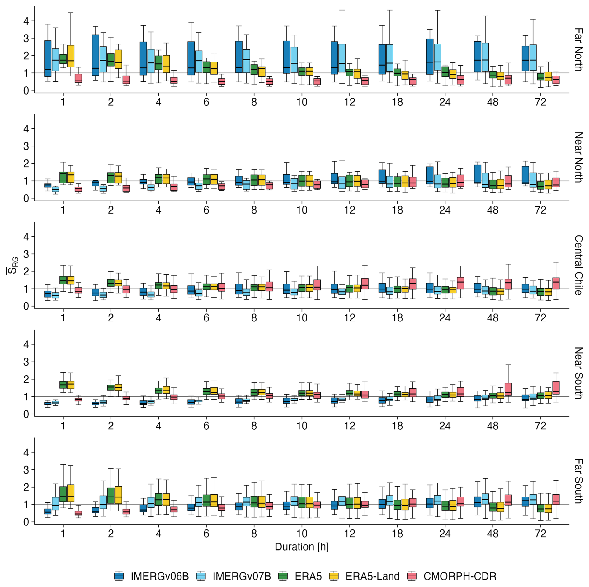
Figure 3 Boxplots summarising annual bias-correction factors (${\stackrel{\mathrm{‾}}{S}}_{d,\text{RG}}$) for each gridded product by macroclimatic zone; for durations of 1, 2, 4, 6, 8, 10, 12, 18, 24, 48, and 72 h.

In all macroclimatic zones but the Far North, most of the gridded datasets -except CMORPH-CDR- showed smaller biases for longer durations. In particular, both IMERG products tended to overestimate I_max at short durations, with median bias correction factors between 0.65–0.82 for 1–6 h, but this overestimation decreased for longer durations, reaching values between 0.92–0.98 for 24–72 h. In contrast, ERA5 and ERA5-Land underestimated I_max at short durations (median bias correction factors in [1.16, 1.49] for 1–6 h). This underestimation decreased with increasing durations, reaching almost unbiased values for 10–12 h (median bias correction factors in [1.04, 1.07]), before shifting to an overestimation for longer durations (median bias correction factors in [0.83, 0.95] for 24–72 h). Nonetheless, in the Far North, where all the rain gauges are at high elevations (above 3000 $\mathrm{m}\mathrm{a}.\mathrm{s}.\mathrm{l}.$), both IMERG products notoriously underestimate I_max for all durations. This underestimation is in agreement with previous studies (Xiong et al., 2025; Chen et al., 2023), specially in mountainous regions, where underestimations of up to 50 % have been reported for IMERGv06B (Rojas et al., 2021). Regarding bias variability, it is larger in the Far North (17 gauges) and Far South (66 gauges) in comparison to the Near North (10 gauges), Central Chile (38 gauges) and the Near South (30 gauges). The following paragraphs describe the biases in I_max obtained in each macroclimatic zone.

In the Far North (17.5–26.0° S), underestimations of I_max for IMERGv06B and IMERGv07B reach median values of ${\stackrel{\mathrm{‾}}{S}}_{d,\text{RG}}$ in [1.2, 1.77]), with larger biases for durations larger than 18 h in the case of IMERGv06B, and similar biases for all the durations for IMERGv07B. On the other hand, ERA5 and ERA5-Land mostly underestimate I_max for durations lower than 8 h (median values of ${\stackrel{\mathrm{‾}}{S}}_{d,\text{RG}}$ in [1.2, 1.74]), show no median bias for durations between 10–24 h, and present a slight overestimation for 48 and 72 h (median values of ${\stackrel{\mathrm{‾}}{S}}_{d,\text{RG}}$ in [0.71, 0.83]). Finally, CMORPH-CDR overestimates I_max for all durations (median values of ${\stackrel{\mathrm{‾}}{S}}_{d,\text{RG}}$ in [0.5, 0.7]).

In the Near North (26.0–32.2° S) and Central Chile (32.2–36.2° S) IMERGv06B and IMERGv07B overestimate I_max for all durations (median values of ${\stackrel{\mathrm{‾}}{S}}_{d,\text{RG}}$ in [0.76, 0.95] and [0.51, 0.86] for IMERGv06B and IMERGv07B, respectively), and smaller median biases for IMERGv06B at expense of a higher dispersion. For both IMERGv06B and IMERGv07B the biases are low for durations larger than 6 h (median values of ${\stackrel{\mathrm{‾}}{S}}_{d,\text{RG}}$ in [0.85, 0.95] and [0.75, 0.86] for IMERGv06B and IMERGv07B, respectively) and increase for shorter durations (median values of ${\stackrel{\mathrm{‾}}{S}}_{d,\text{RG}}$ in [0.76, 0.95] and [0.50, 0.75] for IMERGv06B and IMERGv07B, respectively). On the other hand, ERA5 and ERA5-Land tend to underestimate I_max for durations of 10 h or less in the Near North, and for durations of 24 h or less in Central Chile. As the duration increases, the bias gradually decreases, and for durations greater than 12 h in the Near North and greater than 48 h in Central Chile, ERA5 and ERA5-Land begin to overestimate I_max. Finally, CMORPH-CDR overestimates I_max for all durations in the Near North (median values of ${\stackrel{\mathrm{‾}}{S}}_{d,\text{RG}}$ in [0.56, 0.91]), with the largest bias for durations of 1 and 2 h and the smallest bias for durations of 24 h. In comparison, in Central Chile CMORPH-CDR slightly overestimates I_max for durations equal or shorter than 4 h (median values of ${\stackrel{\mathrm{‾}}{S}}_{d,\text{RG}}$ in [0.85, 0.94]) and progressively underestimates the annual maximum intensities for durations equal or larger than 8 h (median values of ${\stackrel{\mathrm{‾}}{S}}_{d,\text{RG}}$ in [1.06, 1.38]).

In the the Near South (36.4–43.7° S) both IMERGv06B and IMERGv07B overestimate I_max for all durations (median values of ${\stackrel{\mathrm{‾}}{S}}_{d,\text{RG}}$ in [0.55, 0.92]), with slightly lower median biases and dispersion for IMERGv07B. On the other hand, the behaviour of ERA5 and ERA5-Land is just the opposite of the IMERG products, underestimating I_max for all durations (median values of ${\stackrel{\mathrm{‾}}{S}}_{d,\text{RG}}$ in [1.03, 1.72]), with slightly lower biases for ERA5-Land. Finally, CMORPH-CDR slightly overestimates I_max for durations of 1 and 2 h (median values of ${\stackrel{\mathrm{‾}}{S}}_{d,\text{RG}}$ in [0.83, 0.90]) and underestimates I_max for durations equal or larger than 6 h (median values of ${\stackrel{\mathrm{‾}}{S}}_{d,\text{RG}}$ in [1.03, 1.30]), with larger dispersion for durations equal or larger than 18 h.

In the Far South (43.7–56.5° S), IMERGv07B presents lower median biases (median values of ${\stackrel{\mathrm{‾}}{S}}_{d,\text{RG}}$ in [0.94, 1.29]) than IMERGv06B (median values of ${\stackrel{\mathrm{‾}}{S}}_{d,\text{RG}}$ in [0.56, 1.22]), with IMERGv06B overestimating I_max for durations equal or lower than 12 h. In contrast, IMERGv07B only slightly overestimates I_max for one-hour duration events. Again, the behaviour of ERA5 and ERA5-Land is almost the opposite of the two IMERG products, underestimating I_max for durations equal or lower than 8 and 6 h, respectively (median values of ${\stackrel{\mathrm{‾}}{S}}_{d,\text{RG}}$ in [1.07, 1.45]) and slightly overestimating I_max for durations equal or longer than 18 h, in both cases (median values of ${\stackrel{\mathrm{‾}}{S}}_{d,\text{RG}}$ in [0.74, 0.95]). Finally, CMORPH-CDR presents a behaviour similar to IMERGv06B, overestimating I_max for durations lower or equal to 8 h (median values of ${\stackrel{\mathrm{‾}}{S}}_{d,\text{RG}}$ in [0.46, 0.88]) and slightly underestimating it for durations of 48 and 72 h (median values of ${\stackrel{\mathrm{‾}}{S}}_{d,\text{RG}}$ in [1.13, 1.19]). In this macroclimatic zone, most biases are relatively small (median values of ${\stackrel{\mathrm{‾}}{S}}_{d,\text{RG}}$ close to 1) across all durations and products. However, IMERGv06B and CMORPH-CDR exhibit a few outliers with substantial underestimation (median ${\stackrel{\mathrm{‾}}{S}}_{d,\text{RG}}$ values in the range [3.5, 5.5]) for long-duration events. In contrast, ERA5 and ERA5-Land show outliers of similar magnitude to CMORPH-CDR, but these occur for short-duration events (1–2 h).

The higher variability in gridded precipitation biases in the Far North and Far South of Chile likely arises from the combination of complex orography, sparse observational networks, and the nature of precipitation processes in these regions. In the Far North, precipitation is highly sporadic and convective (e.g. Garreaud, 1999), often associated with isolated storms and strong topographic gradients, which are challenging for coarse-resolution or satellite-based products to capture accurately. In the Far South, precipitation is dominated by frontal systems with cold cloud-tops and marked orographic enhancement over the austral Andes (Viale and Garreaud, 2015), producing highly spatially variable precipitation that may not be fully resolved by the spatial resolution of ERA5 or IMERG. In contrast, Central Chile exhibits more frequent and spatially uniform precipitation events (Falvey and Garreaud, 2007), which are easier for gridded products to represent, resulting in lower bias variability

4.2 Spatial interpolation of bias-correction factors

To move from the ${\stackrel{\mathrm{‾}}{S}}_{d,\text{RG}}$ values obtained at point locations in the previous section into a spatially continuous field, we first followed Ombadi et al. (2018) and investigated whether there is a relationship between the bias in I_max and elevation or not, finding no clear correlation between both variables (R²<0.3, see Supplement S3 in Soto-Escobar et al., 2025). Based on this result, we discarded implementing a bias correction based on elevation.

Second, we interpolated the bias-correction factors using thin-plate splines (Karger et al., 2021), which produced the most realistic maps compared to alternative methods like inverse distance weighting and bilinear interpolation. Unlike the other methods, the thin-plate spline interpolation provided a smoother and more balanced surface, without abrupt bias changes or convergence issues. The bias-correction factors were interpolated using the values from 144 rain gauges located in all the study areas but the Far North (see Supplement S1 in Soto-Escobar et al., 2025), obtaining specific bias-correction maps for each product and duration (see Supplement S4 in Soto-Escobar et al., 2025). In the data-scarce and hyper-arid Far North we chose not to provide maps of annual maximum intensities, because the bias-correction factors were derived exclusively from hourly rain gauges located above 3000 $\mathrm{m}\mathrm{a}.\mathrm{s}.\mathrm{l}.$ The current absence of hourly precipitation data in the Far North highlights the need to increase the density of rain gauges in hyper-arid areas, where a few extreme precipitation events can trigger important damages to civil population and infrastructure (e.g. Hauser, A, 1997; Vargas et al., 2000; Wilcox et al., 2016).

4.3 Trends in I_max

For all the gridded datasets, Supplement S5.2 (Soto-Escobar et al., 2025) contains maps showing Kendall's τ values statistically significant at α=0.01, α=0.05, and α=0.10; as well as maps with all the computed trends independent of their statistical significance. Although the trend areas are somewhat smaller at lower significance levels, such as α=0.01, the spatial distribution of areas with statistically significant trends remains the same. In general, for all durations the results of the trend analysis were similar between ERA5 and ERA5-Land, as well as for IMERGv06B and IMERGv07B. In addition, the trends obtained for ERA5 and ERA5-Land were also similar when using 20 (2001–2021) and 40 (1981–2021) years of data length, although with slightly smaller areas with significant trends in the latter case. Therefore, Fig. 4 only shows Kendall's τ for all gridded products for 2001–2021, where cells with green (orange and red) colour represent increasing (decreasing) trends, and white cells indicate the absence of a statistically significant τ value at α=0.05.

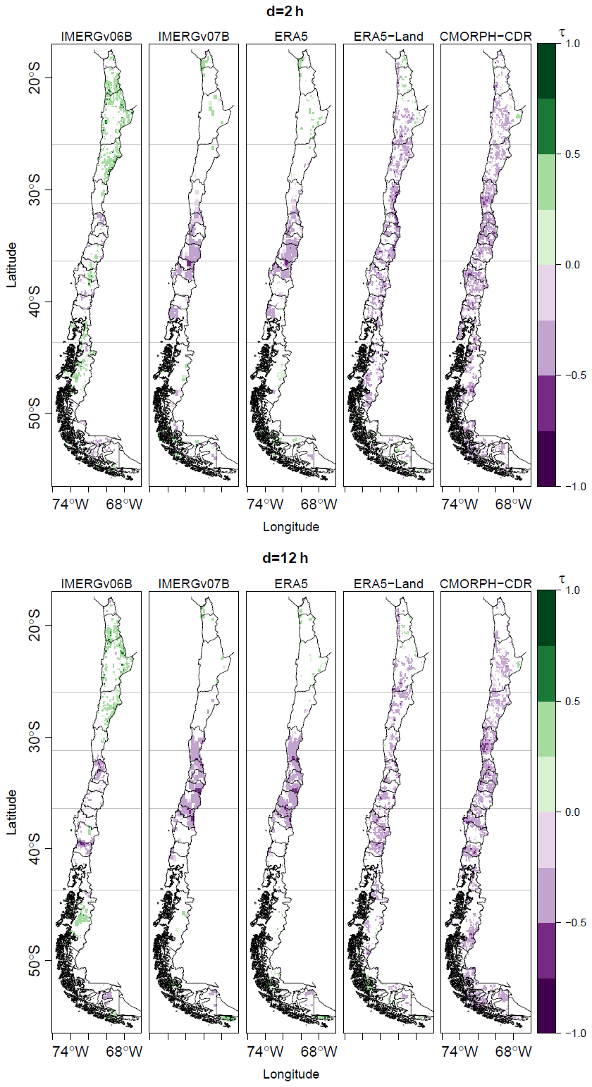
Figure 4 Kendall's Tau (τ) for all gridded datasets for 2001–2021. Positive (negative) values indicate an increasing (decreasing) trend. White cells indicate that τ was not statistically significant at α=0.05.

Figure 4 shows that IMERGv07B presents isolated increasing trends for both 2 and 12 h durations in the Near North (τ values in [0.2, 0.68]), and decreasing trends from 32.4 to 34.6° S (Valparaíso and Metropolitana regions) in Central Chile (τ values in [−0.2, −0.5]), with a larger area with decreasing trends as the duration increases, which similar for all durations. In the Near South, IMERGv07B shows almost no trend for the 2 h duration, a pattern that remains similar for durations up to 8 h; for 12 h and longer, it presents decreasing trends (τ values in [−0.2, −0.7]). In the Far South, only isolated increasing trends are observed for all durations. On the other hand, ERA5-Land shows decreasing trends in the Near North for the 12 h duration (τ values in [−0.1, −0.4]), a behaviour that is also observed for durations between 6–72 h. For all durations from Valparaíso to the Biobío regions (32–38° S), decreasing trends are observed (τ values in [−0.3, −0.68]), and there are no significant trends for any duration south of 38° S. Finally, CMORPH-CDR shows decreasing trends for all durations and across the entire continental area of Chile (τ values in [−0.2, −0.78]).

The results of the modified Mann–Kendall trend test for the 20 and 40 year periods revealed large areas with no trends, as well as a predominant decreasing behaviour of I_max, which is observed for all products and durations in Central Chile. IMERGv07B showed increasing trends for isolated areas of Near North and Far South, contrary to the decreasing or no trends obtained for ERA5-Land and the decreasing trends found in CMORPH-CDR in the same areas.

In contrast to studies that suggest an increase in extreme precipitation intensities worldwide due to rising temperatures (Trenberth, 1999; Allen and Ingram, 2002; Pall et al., 2007; Fowler et al., 2021a, b; Neelin et al., 2022), our results show that I_max is decreasing in Chile, a pattern that is also observed in other regions of the world (Liu et al., 2005; Utsumi et al., 2011; Serrano-Notivoli et al., 2018). This decrease in I_max could be due to the fact that non-stationarity is only applied to the location parameter of the Gumbel distribution, as discussed by Prosdocimi and Kjeldsen (2021) using a three-parameter GEV distribution with data from 40 streamflow stations spanning 65–115 years. However, we are confident that the decrease in I_max is likely due to the decreasing number of winter storms (cold fronts) that have reached central Chile in recent decades (Garreaud et al., 2019). Our results are consistent with the observed decrease in daily precipitation records from 1979 to 2017 in all seasons except summer (Lagos-Zúñiga et al., 2024). The decrease in I_max is also consistent with a strong drying trend (in terms of annual accumulation) registered in central and southern Chile in 2010–2022, partly due to climate change (Boisier et al., 2018) and strongly influenced by the Chilean megadrought (Garreaud et al., 2017). However, the wet years 2023 and 2024 (outside the temporal period of our analysis) could potentially change these observed trends. On the other hand, the global models also project a slight decrease in precipitation extremes for the Near North and Central Chile for 2075–2099 compared to 1990–2014, despite a global increase in precipitation extremes (Martinez-Villalobos and Neelin, 2023). In particular, Martinez-Villalobos and Neelin (2023) projects a strong increase in extreme events for the Far North. Unfortunately, we did not provide I_max values for this region due to the sparse network of sub-daily rainfall records.

Our results also indicate that the decreasing trends in I_max for durations longer than 24 h are consistent with those observed for shorter durations, suggesting that trends in precipitation intensities persist across different temporal scales.

4.4 I_max derived from the stationary model

Based on bias-corrected annual maximum intensities, we obtained I_max using stationary and non-stationary models for durations of 1, 2, 4, 6, 8, 10, 12, 18, 24, 48, and 72 h and return periods of 2, 5, 10, 25, 50, and 100 years. Due to the large number of figures involved in the previous analyses, and the similarity in I_max from the stationary and non-stationary model (see Sect. 4.5), Fig. 5a and c only shows maps of I_max values derived from stationary model, in mm h⁻¹, for a 50 years return period and durations of 2 and 12 h, as representative of important storms affecting Central-Southern Chile. Additionally, in this figure, IMERGv06B is excluded to emphasise IMERGv07B, the latest version of the product, while ERA5 is not included due to its similarity to ERA5-Land. Supplements S7 and S8 (Soto-Escobar et al., 2025) contain boxplots and maps, respectively, with I_max values obtained from the stationary and non-stationary models, for all gridded datasets, all durations and all return periods. In all these maps the hyper-arid Far North (17.5–26.0° S) has been intentionally removed, due to unrealistic I_max values created by the interpolation of the bias-correction factors (see details in the Supplement S4 in Soto-Escobar et al., 2025).

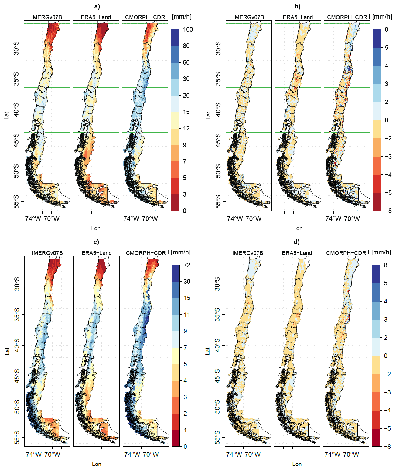
Figure 5 Panels (a) and (c) show maps of I_max derived from the stationary model for the IMERGv07B, ERA5-Land, and CMORPH-CDR, for a 50 year return period: panel (a) shows results for the 2 h duration, and panel (c) for the 12 h duration. Panels (b) and (d) present maps of the differences in I_max between the non-stationary and stationary models for the same datasets and return period, with 2 h duration in panel (b), and 12 h duration in panel (d).

Figure 5 and the Supplement S8.1 (Soto-Escobar et al., 2025) show that the spatial distribution and numerical values of I_max shown by IMERGv07B are very similar to those obtained from ERA5 and ERA5-Land, for all durations. At the same time, IMERGv06B shows higher I_max values than the three previous products, and CMORPH-CDR shows the highest values among all precipitation datasets, especially in the Andes Cordillera. As expected, the highest I_max values are obtained for the shortest durations, for all products. For d=1 h, IMERGv06B shows a larger spatial area with high I_max values than IMERGv07B, but this difference increasingly disappears for longer durations. For all return periods and for durations of 1 and 2 h, the highest I_max values are distributed from Central Chile throughout to the Austral Patagonia. For durations of 4 h or longer, however, these highest I_max values are only concentrated in Central and Southern Chile (32.2–43.7° S). For precipitation events with a duration of 12 h or longer, Central and Southern Chile show two different patterns: from 32.4 to 34.6° S (Valparaíso and Metropolitana regions), the annual maximum intensities occur along the coast, while between 34.6–36.4° S these maximum intensities shift towards the Andes, with weaker intensities on the coast.

On the other hand, for all products, the difference in I_max between the Andes and the intermediate depression/western Pacific border becomes more pronounced with increasing duration. For durations of 24 h or more, the highest intensities are mainly concentrated in the Andes, from the Maule to the Araucanía region (35–40° S). An exception to this pattern is the coastal area of the Bio-Bio region (∼37° S), which is dominated by the Nahuelbuta mountains (with elevations over 1200 $\mathrm{m}\mathrm{a}.\mathrm{s}.\mathrm{l}.$), which are responsible for much higher precipitation values than the surrounding lowlands (Garreaud et al., 2016). The large longitudinal differences in the I_max values emphasise the importance of using a spatially explicit representation of precipitation intensities in civil infrastructure design, stormwater management, and flood risk assessment. Furthermore, the intensities observed in the intermediate depression are not representative of those in the Andes. Recently, Abarca et al. (2024) calculated the accumulated precipitation over six hours triggering societal impacts in Central Chile during the 8 year period 2015–2022. Our I_max values for a 6 h duration and 10 year return period resulted in accumulated precipitation values exceeding the warning thresholds given by Abarca et al. (2024) in all geomorphological units.

Interestingly, this is the first work showing how the spatial distribution of I_max differs from the distribution of mean annual precipitation in continental Chile (Fig. 1). While mean annual precipitation increases almost monotonically from the Far North towards southern Patagonia, for all durations I_max presents its maximum values in Central-Southern Chile (32.2–43.7° S).

To provide a quantitative summary of the differences in annual maximum intensities across all gridded datasets, Fig. 6 shows boxplots summarising the I_max values for each gridded dataset for T=50 years and durations of 1, 2, 6, 12, 24, 48, and 72 h, aggregated by macroclimatic area. Supplement S7 (Soto-Escobar et al., 2025) contains boxplots for all gridded datasets, durations and return periods.

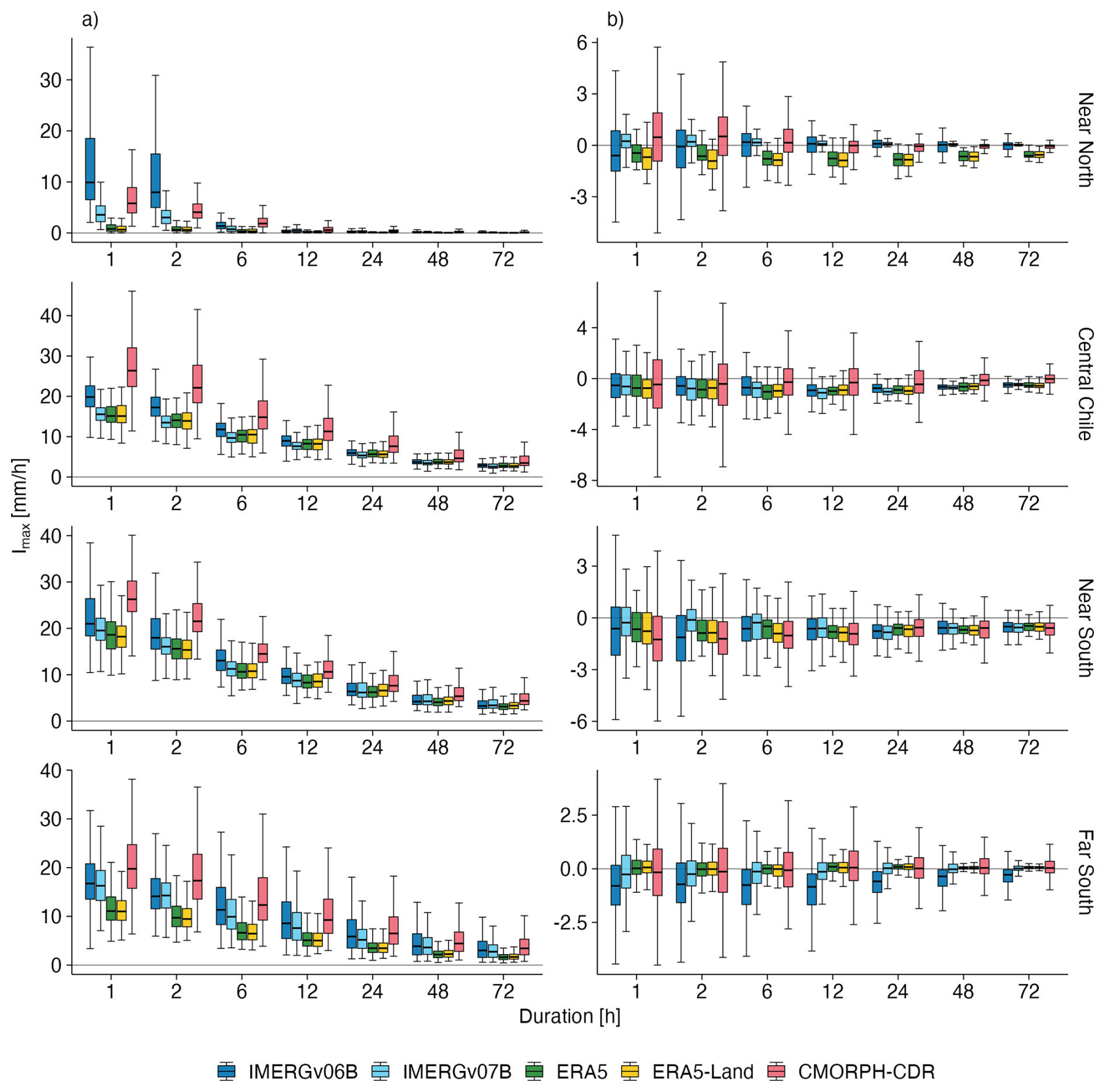
Figure 6 Boxplots of I_max for all gridded datasets and climatic macrozones, corresponding to a 50 year return period and durations of 1, 2, 6, 12, 24, 48, and 72 h. Panel (a) shows the values derived from stationary models, while panel (b) presents the differences in I_max between non-stationary and stationary models, for the same datasets, climatic macrozones, and durations.

In general, Fig. 6 shows that for all macroclimatic areas the highest intensity values are provided by CMORPH-CDR, followed by IMERGv06B. These two products are also the ones with the largest amount of outliers for all durations, with CMORPH-CDR always having more outliers than IMERGv06B in any macroclimatic area. For CMORPH-CDR, the amount of outliers is largest in Central Chile (32.2–36.2° S) and the Near South (36.4–43.7° S), while in the case of IMERGv06B the largest amount of outliers is observed in the Near South followed by the Far South (43.7–56.5° S). In the case of CMORPH-CDR, the large number of outliers (Fig. 6) would indicate either a high spatial variability of I_max (which we can not discard or confirm with the current density of rain gauges), or a low ability of this product to reproduce the annual maximum intensities.

Figure 6 shows a strong agreement among the I_max values derived from IMERGv07B, ERA5 and ERA5-Land, from the Near North to the Near South (26.0–43.7° S), while in the Far South (43.7–56.5° S), IMERGv07B presents slightly higher annual maximum intensities for all durations. Overall, despite important differences between their origin, we obtained similar I_max values for IMERGv07B, ERA5 and ERA5-Land, mainly for Central and Southern Chile (32.2–43.7° S), which concentrate the highest amount of rain gauges. The convergence of I_max between the satellite-based IMERGv07B product and those resulting from reanalyses (ERA5 and ERA5-Land) increases our confidence in the I_max values provided by these three datasets.

Although not directly comparable due to differences in the dataset, temporal period of analysis and methodology used, our I_max values obtained for a duration of 24 h and a return period of 10 years are similar to the isohyets values used as reference in Chile until today (DGA, 1991). Similarly, our I_max values obtained for return periods of 2, 5, 20, 50, and 100 years are close to those derived from DGA (1995) using frequency and duration factors. Supplement S10 (Soto-Escobar et al., 2025) shows that the IDF curves obtained after bias-correction are similar to those derived from in situ rain gauge data, demonstrating the efficiency of the bias-correction method, despite the challenge of having a low number of stations and relatively short observed data length.

Finally, in the Supplement S11 (Soto-Escobar et al., 2025) we also compared our annual maximum intensities (in mm h⁻¹) with those of the Precipitation Probability DISTribution (PPDIST) product (Beck et al., 2020), which provides values for return periods ranging from 3 d to 15 years, considering 3 h and daily events. For T=10 years and a duration of 3 h, all PPDIST values were in general higher (∼5–10 mm h⁻¹) than those of IMERGv06B, IMERGv07B, ERA5 and ERA5-Land, and where mostly lower than those of CMORPH-CDR (∼2–5 mm h⁻¹). These higher I_max in PPDIST could be attributed to the lack of hourly rainfall gauges in PPDIST for continental Chile. On the other hand, for T=10 years and a duration of 24 h all PPDIST values were similar to those provided by IMERGv06B, IMERGv07B, ERA5 and ERA5-Land (median values of all these products in [3.3, 4.1] mm h⁻¹), and slightly lower than those derived from CMORPH-CDR (median value of 4.8 mm h⁻¹).

4.5 Comparison of I_max from non-stationary vs stationary models

To facilitate the comparison of the I_max obtained with the stationary and non-stationary models of extreme rainfall, Figs. 5 and 6 show maps and boxplots, respectively, of I_max differences for various durations and T=50 years across all grid cells belonging to each macroclimatic region, calculated as non-stationary minus stationary values. These figures use all the cells with a statistically significant τ value at α=0.05. Supplement S8 show I_max obtained from stationary and non-stationary models for other return periods for all the gridded precipitation datasets used in this study.

In Fig. 5b and d, blue (yellow, orange, red) colours indicate that the values estimated from non-stationary are higher (lower) than their stationary counterparts. The predominance of the yellow colour in this figure indicates that, in general, intensities from the non-stationary model are slightly lower than their stationary equivalents (differences in [0, 5] mm h⁻¹). Some isolated exceptions for the previous finding are localised in the Near North (26.0–32.2° S) and Austral South (43.7–56.5° S) for durations equal or higher than 12 h, and all along the country for short precipitation events (d=1 h). The differences between the non-stationary and stationary models become smaller for longer durations (greater than 8 h), which aligns with findings from Ganguli and Coulibaly (2017).

On the other hand, Fig. 6 shows that the median differences between I_max estimated using the non-stationary and stationary models are consistently shifted towards negative values, confirming that the non-stationary I_max values are slightly lower than their stationary counterparts (median differences in [0, 1] mm h⁻¹). Only three exceptions where the median differences are higher or close to zero were found: (i) IMERGv07B in the Near North (26.0–32.2° S); (ii) CMORPH-CDR in the Near North and Far South (43.7–56.5° S), and (iii) ERA5 and ERA5-Land in the Far South.

In addition, Fig. 6 also shows that the median differences between I_max based on the non-stationary and stationary models are close to zero for all gridded datasets (median values in [0, 2] mm h⁻¹), and the dispersion around these median values generally decrease with increasing durations. It is worth mentioning that, in the Far South (43.7–56.5° S), ERA5 and ERA5-Land present almost no differences between I_max values obtained under stationary and non-stationary assumptions, with median values very close to zero and the interquantile range (q97–q25) in [−0.5, 0.5] mm h⁻¹.

Finally, Fig. 6 shows that the variability of the difference between non-stationary and stationary models is very low for all durations, with the interquantile range (q97–q25) in [−2, 2] mm h⁻¹. CMRORPH-CDR is the product with the largest amount and largest absolute values of outliers for all durations, while IMERGv06B and IMERGv07B present similar median differences in I_max derived from both models, but with much lower variability in the case of IMERGv07B. ERA5 and ERA5-Land exhibited similar median differences and variability.

To further assess the statistical similarity between stationary and non-stationary models, Fig. 7 presents scatter plots of the estimated values for each product and region. The strong clustering of points along the 1:1 line across all panels indicates a high degree of agreement between the two approaches throughout the full distribution of annual maxima. A slight tendency for I_max from the non-stationary model to be lower, particularly for the most extreme values, supports the systematic negative differences identified in the boxplot analysis (Fig. 6). IMERGv07B, ERA5, and ERA5-Land exhibit particularly high consistency between the modelling approaches, with minimal scatter. By contrast, IMERGv06B and CMORPH-CDR display greater variability, especially in regions characterised by more intense precipitation, such as the Near North and Far South. Despite these discrepancies, the differences introduced by the (non-)stationary modelling assumption remain small relative to the magnitude of the I_max extremes. Overall, the scatter plots confirm that the observed differences are systematic across the full range of values rather than driven by spatial climatological gradients. They complement the boxplot results and show that non-stationary modelling generally introduces only minor adjustments to extreme precipitation estimates for most datasets and regions

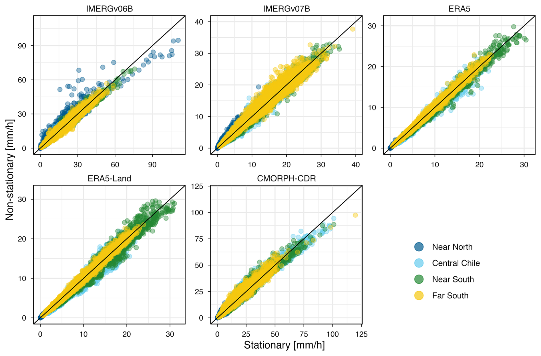
Figure 7 Scatterplots comparing I_max derived from stationary and non-stationary model for each product and all durations. Points are coloured by climatic macrozone, and the 1:1 line indicates perfect agreement between both approaches.

In conclusion, our findings indicate that locations with a statistically significant trend in I_max do not necessarily exhibit significant differences between I_max values derived from stationary and non-stationary models. Therefore, while accounting for the non-stationarity of extreme precipitation is important, observed trends can also be captured by stationary models when using time-dependent parameters or flexible probability distributions (Dimitriadis et al., 2021), consistent with findings from Ganguli and Coulibaly (2017), Yilmaz et al. (2014), Yilmaz and Perera (2014). In addition, Dimitriadis et al. (2021), Dong et al. (2021) further showed that stationary models incorporating flexible distributions or temporal correlation can reproduce observed trends and long-term persistence in precipitation extremes.

4.6 Impact of data length on I_max

For each grid cell of ERA5 and ERA5-Land, we compared the I_max values estimated with 40 and 20 years of data using both stationary and non-stationary approaches for return periods of 2, 5, 10, 25, 50, and 100 years. Figure 8 focuses on the case of T=50 years, summarising the differences $I_{\text{max},\mathrm{40}\mathrm{years}}-I_{\text{max},\mathrm{20}\mathrm{years}}$ for both approaches. Our results show median differences close to 0 mm h⁻¹, interquartile ranges within (−1, 1] mm h⁻¹, and maximum differences within [−4, 4] mm h⁻¹ across all durations and macroclimatic zones. Readers interested in other return periods can find similar results in the Supplements S9.1 and S9.2 in Soto-Escobar et al. (2025).

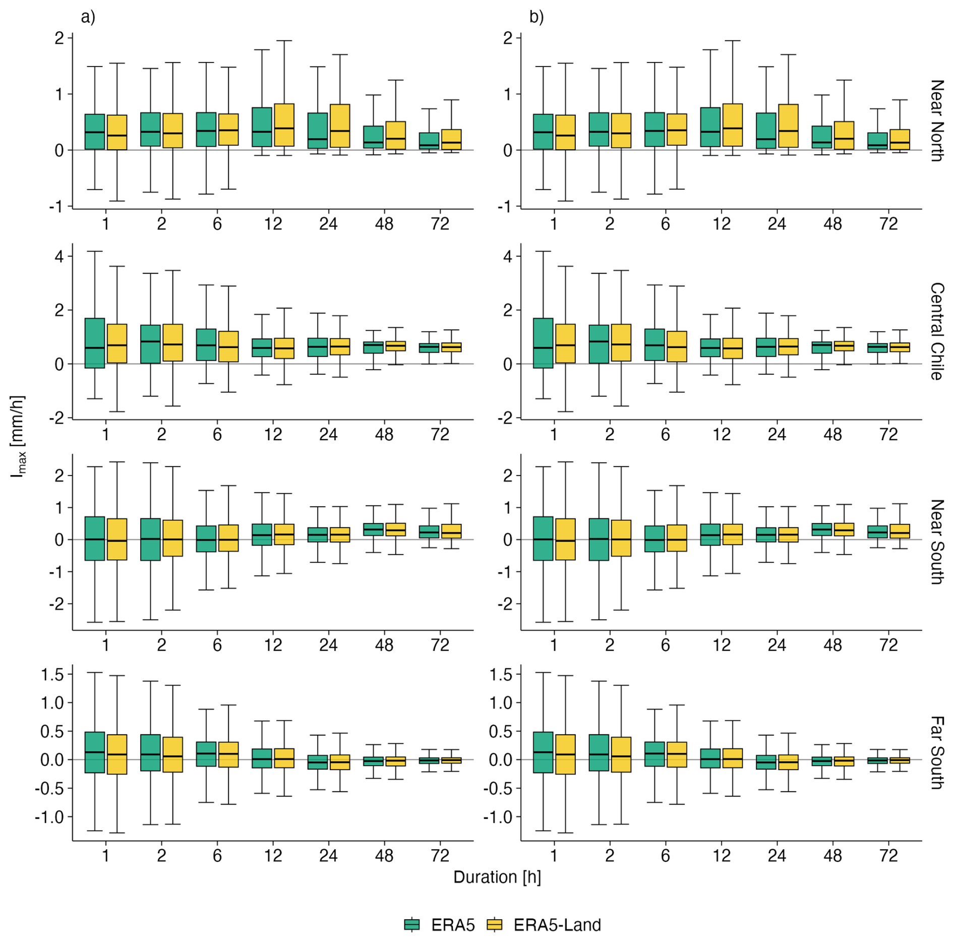
Figure 8 Boxplots summarising differences between I_max derived from stationary and non-stationary models, estimated using data series of 40 and 20 years ($I_{\text{max},\mathrm{40}\mathrm{years}}-I_{\text{max},\mathrm{20}\mathrm{years}}$), for ERA5 (green colour) and ERA5-Land (yellow colour), considering a 50 years return period and durations of 1, 2, 6, 12, 24, 48, and 72 h. From top to bottom, each panel corresponds to a different macroclimatic area. Column (a) shows results obtained using the stationary model, while column (b) shows results from the non-stationary model.

The smallest differences were found in the Near North (26.0–32.2° S) and Far South (43.7–56.5° S), where the median differences were almost 0 mm h⁻¹, the interquartile values were in [−0.5, 0.5] mm h⁻¹, and almost all the largest differences were in [−2, 2] mm h⁻¹ for all durations. In Central Chile (32.2–36.2° S), for both ERA5 and ERA5-Land, there were almost no differences in I_max for d=48 and d=72 h, with a median value of practically 0 mm h⁻¹ in both cases, and all the differences in [−0.5, 1] mm h⁻¹; while for durations d=1 and d=2 h the median differences were slightly positive (in [0.1, 0.2] mm h⁻¹), with a larger spread (mostly in [−3, 4] mm h⁻¹); and for durations of 6, 12, and 24 h the median differences were slightly negative (in [−0.1, −0.2] mm h⁻¹), with a relatively small spread (mostly in [−2, 1.5] mm h⁻¹). In the Near South (36.4–43.7° S), the differences obtained between ERA5 and ERA5-Land were very similar to the ones obtained for Central Chile, with the exception of the very short durations. For d=1 and d=2 the median differences were slightly negative (in [−0.1, −0.2] mm h⁻¹), with a spread mostly in [−4, 4] mm h⁻¹.

Our results align with Marra et al. (2017), who found that the uncertainty in the estimated parameters of the GEV distribution is particularly pronounced in arid climates and for short durations, likely due to the limited number of rainfall events considered in each year. This result suggests that time aggregation may help mitigate some of the challenges of using short data records. Our findings also align with Ombadi et al. (2018), who mentioned that short data records can be associated with increasing errors in I_max for increasing return periods, when introducing a new framework to develop IDF curves over the contiguous United States based on daily PERSIANN-CDR data.

Figure 9 presents representative maps of the percentage differences in the location and scale parameters of the stationary Gumbel distribution for ERA5-Land, comparing estimates obtained with 20 years (2001–2021) and 40 years (1981–2021) of data. The differences were computed by subtracting the 20 year parameter estimates from the 40 year estimates and then normalising by the 40 year values. The results show generally minor differences in the location parameter (−10 %–10 %) across the study area for both ERA5 and ERA5-Land, with the exception of the coastal area of the Coquimbo region (26–30° S), where differences reach up to −40 %. By contrast, the scale parameter exhibits larger differences (−40 %–40 %) throughout the domain. These include a clear spatial pattern of higher values for the 20 year period in most of the Near North (26.0–32.2° S) and Central Chile (32.2–36.2° S), and a more heterogeneous “salt and pepper” pattern in the South (36.4–43.7° S) and Far South (43.7–56.5° SS) macrozones. Readers interested in the raw maps of the Gumbel parameters for the stationary model can find them in the Supplement S6.1 (Soto-Escobar et al., 2025).

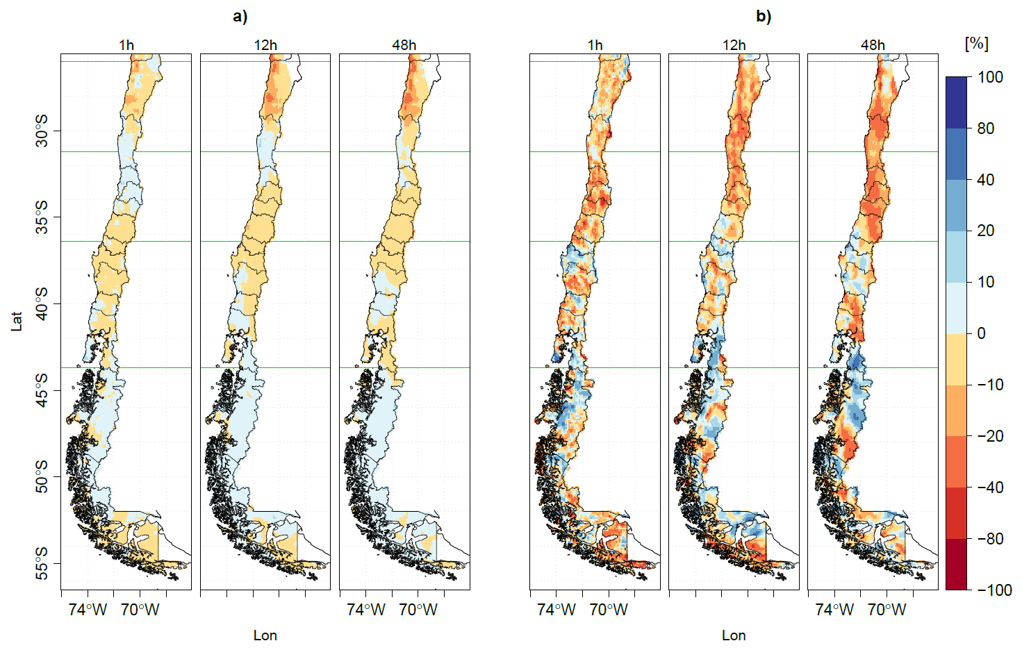
Figure 9 Panel (a) presents maps of the percentage difference in the location parameter between the periods 1981–2021 and 2001–2021 using the ERA5-Land dataset. Panel (b) shows maps of the percentage difference in the scale parameter for the same periods, based on the ERA5 dataset. Results are provided for rainfall durations of 1, 12, and 48 h.

Despite the previous differences in the Gumbel parameters, we obtained only minor differences (median values lower than 1 mm h⁻¹) in the I_max derived from 20 and 40 years of data, both for ERA5 and ERA5-Land, as shown in Fig. 8 for the stationary and non-stationary models.

Our findings complement results obtained by Papalexiou and Koutsoyiannis (2013), who found that the data length used in the frequency analysis had an important effect in the values of the shape parameter, when the 3-parameter GEV is used instead of the 2-parameter Gumbel distribution. In addition, their analysis was based on data lengths ranging from 40 to 163 years, making their findings not directly comparable to ours.

Endreny and Imbeah (2009) used data from the Tropical Rainfall Measuring Mission (TRMM) processed by the 3B42 algorithm with precipitation records every 3 h from the Ghana Meteorological Service Department (GMSD), combining both records for the generation of IDF curves in Ghana, obtaining good results, but limited by the TRMM temporal resolution of 3 h. Although these results are not directly comparable to ours; due to differences in study areas, satellite products, temporal periods, and methodologies; they suggests that combining station data and satellite products is essential for generating IDF curves, which aligns with our findings.

Although not directly comparable to our study due to substantial differences in data length and methodology, Iliopoulou and Koutsoyiannis (2019) highlighted that the length of the precipitation time series can have an important influence on extreme precipitation values when using stationary models, due to the long-term persistence observed in precipitation time series.

4.7 curvasIDF: a web platform for IDF curves in Chile

For each grid cell of each precipitation dataset is possible to obtain a figure with the I_max values obtained in this work, for different durations and return periods. However, presenting such a large number of figures in a single document is not feasible from a practical point of view, not even in the Supplement. Therefore, we implemented a user-friendly web platform (https://curvasIDF.cl/, last access: 18 December 2025), where the interested reader can define a duration and return period of interest and then click at any point of the study area to obtain the corresponding IDF curves for all the gridded datasets used in this work. We made an important effort into developing this web platform to make it easier for practitioners and decision makers to obtain IDF curves for designing climate-resilient infrastructure and managing the impacts of climate change on water resources.

5 Conclusions

To overcome the limited availability of long time series of in situ sub-daily precipitation data, we use five state-of-the-art hourly precipitation datasets (IMERGv06B, IMERGv07B, ERA5, ERA5-Land, CMORPH-CDR) and 161 quality-checked hourly rain gauges to compute stationary and non-stationary annual maximum intensities (I_max) and IDF curves for the climatologically and topographically diverse Chilean territory (17–56° S).

To the best of our knowledge, this is the first work comparing annual maximum intensities derived from stationary and non-stationary statistical models and from two different families of state-of-the-art gridded precipitation datasets: IMERGv06B/IMERGv07B and ERA5/ERA5-Land. In particular, this is the very first study providing intensity-duration-frequency curves at high spatial and temporal resolution using state-of-the-art gridded precipitation datasets for continental Chile. This constitutes an important contribution to advancing our knowledge about extreme precipitation events in mountainous areas where such information is generally unavailable.

Our key findings are summarised in the following lines:

• The biases in I_max varied depending on the gridded precipitation product, the macroclimatic zone and the duration considered in the analysis. In general, most gridded datasets –except CMORPH-CDR– showed smaller biases for longer durations. IMERG products consistently overestimated short-duration extremes (1–6 h) but improved toward near-unbiased estimates at longer durations (24–72 h), whereas ERA5 and ERA5-Land shifted from slight underestimation at short durations (1–6 h) to slight overestimation at longer durations (24–72 h). Bias variability is greater in the extreme Far North and Far South, as compared to the more central macroclimatic zones.

• This is the first study showing how the spatial distribution of the annual maximum intensities (I_max) derived from stationary and non-stationary models differs from the distribution of the spatial pattern of mean annual precipitation in continental Chile. While mean annual precipitation increases steadily southward, I_max reaches its maximum values in Central-Southern Chile, for all durations. For durations of 24 h or more, the highest intensities are primarily found in the Andes, particularly between the Maule and Araucanía region (35–40° S).

• There is a high longitudinal gradient in I_max, from the low values in the intermediate depression to the high values in the Andes, which increase with larger durations. This is particularly relevant for the design of civil infrastructure, stormwater management and for flood risk assessment in Chile: intensities measured in the intermediate depression (typical of current design manuals) are not representative of I_max in the Andes.

• Despite important differences in their technical foundations, for all durations, IMERGv07B closely matches ERA5 and ERA5-Land in spatial distribution and I_max values. IMERGv06B shows higher I_max values, while CMORPH-CDR has the highest, especially in the Andes cordillera.

• The largest intensity values are provided by CMORPH-CDR, followed by IMERGv06B for all macroclimatic areas, and these two products have the largest amount of outliers for all durations.

• In Central Chile, all precipitation products revealed either significant decreases in I_max (at α=0.01, α=0.05, and α=0.10) or no detectable trends. While the extent of significant areas was smaller at the stricter level (α=0.01), their spatial distribution remained consistent across significance levels. For ERA5 and ERA5-Land, these declining trends were evident in both 1981–2021 and 2001–2021, whereas the other products were only available for the shorter 2001–2021 period. In contrast, regional differences emerged outside Central Chile: in the Near North and Far South, IMERGv07B displayed localised increases, ERA5-Land showed mostly decreases or no trends, and CMORPH-CDR consistently indicated widespread declines.

• In general, for all durations and most of the gridded precipitation datasets, the non-stationary I_max values are slightly lower than their stationary equivalents (differences in [0, 5] mm h⁻¹), and the differences between the non-stationary and stationary I_max become smaller for longer durations (greater than 8 h). This result suggests that the choice between stationary and non-stationary approaches should be carefully analysed for each study area, and for the Chilean case study it does not significantly affect the estimation of I_max values. In addition, locations with a significant trend in I_max will not necessarily exhibit significant differences between stationary and non-stationary I_max.

• When comparing the Gumbel parameters derived from ERA5 and ERA5-Land using 20 year (2001–2021) and 40 year (1981–2021) data under the stationary assumption, we found minor differences (−10 %–10 %) in the location parameter across the study area for both datasets. In contrast, the scale parameter exhibited larger differences, ranging from −40 % to 40 %.

• Despite the previously noted differences in the Gumbel parameters, the resulting I_max values derived from 20- and 40 year records show only minor differences (median values below 1 mm h⁻¹) for both ERA5 and ERA5-Land, across all durations and for both the stationary and non-stationary cases.

6 Practical recommendations

To provide practical guidance for hydrological and engineering applications that require a reliable quantification of extreme precipitation events in Chile, we make the following recommendations:

• We encourage the Chilean Water Directorate (DGA) to increase the number of hourly rain gauges in mountainous areas, which are fundamental to assessing the behaviour of gridded precipitation products. We also encourage the National Agroclimatic Network (Agromet) to apply quality control algorithms to ensure the reliability of their hourly precipitation time series (e.g. Blenkinsop et al., 2017).

• Given the convergence between I_max obtained from ERA5, ERA5-Land and IMERGv07B, we recommend using the highest value among them for designing safer climate-resilient infrastructure.

• Given the large amount of spatially explicit I_max for different durations and return periods, all our results are publicly available in a user-friendly web platform: https://curvasidf.cl (last access: 18 December 2025).