Uncertainty, temporal variability, and influencing factors of empirical streamflow sensitivities

The sensitivity of streamflow to changes in driving variables such as precipitation and potential evaporation is a key signature of catchment behaviour. Due to increasing interest in climate change impacts, streamflow sensitivities derived from observations have become a widely used metric for catchment characterization, model evaluation, and observation-constrained projections. However, there remain open questions regarding the robustness and temporal variability of empirically-derived sensitivities. In this paper, we revisit theoretical and empirical approaches to estimate streamflow sensitivities to precipitation and potential evaporation. First, we compare different estimation methods, primarily based on linear regression, using a synthetic dataset for which the sensitivities are known. Second, we extend this comparison and use two methods selected based on the previous analysis to estimate sensitivities for >1000 near-natural catchments. Third, we investigate how sensitivities change over time due to changes in the ratio between potential evaporation and precipitation (i.e., aridity index). Our results confirm that multiple regression is preferable to single regression, but that in presence of noise and correlation between precipitation and potential evaporation, even multiple regression methods can lead to high uncertainty, especially for potential evaporation. When analysing real catchments, sensitivity to precipitation is estimated consistently across methods, while sensitivity to potential evaporation is highly uncertain and often yields unrealistic values. Further, as the aridity index increases over time – a trend found in observational data – sensitivities decrease (by 15 %–70 % over 50 years) and can thus not be viewed as static. Empirical sensitivities, as well as their trends, relate strongly to the aridity index, but are also influenced by other factors, especially those related to catchment storage processes, as well as data uncertainty. Our results should urge caution in the use of empirical streamflow sensitivities for climate change impact assessments and call for further investigation.

1 Introduction

In response to ongoing interest in climate change impacts, the sensitivity of streamflow to changes in climatic drivers has received considerable attention in recent years (e.g., Andréassian et al., 2016; Lehner et al., 2019; Zhang et al., 2023). In particular, sensitivities to precipitation, temperature, and potential evaporation are commonly used, though the concept can be extended to other driving variables that influence streamflow, such as storage (e.g., Berghuijs et al., 2016; de Lavenne et al., 2022; Weiler et al., 2025; Zhang et al., 2023) or land cover changes (e.g., Anderson et al., 2022; Roderick and Farquhar, 2011; Steinschneider et al., 2013).

Sensitivity is defined as the change in streamflow per unit change in a certain driving variable. This can be expressed in absolute terms (e.g., by how many mm streamflow changes per mm change in precipitation) or in relative terms (e.g., by how many %-points streamflow changes per 1 % change in precipitation), the latter often being called elasticity (Andréassian et al., 2016; Sankarasubramanian et al., 2001). We will define both terms more formally later on.

One of the earliest studies explicitly mentioning the “sensitivity of water resource systems to climate variations” was by Němec and Schaake (1982), who used the Sacramento Soil Moisture Accounting model to estimate sensitivity of streamflow to changes in precipitation and potential evaporation for two contrasting basins (an arid and a humid one). This approach comprises one typical category of sensitivity studies, namely perturbation experiments using (process-based) simulation models of varying complexity (e.g., Němec and Schaake, 1982; Nijssen et al., 2001; Schaake, 1990). Another category are simple Budyko-type water balance models (Budyko, 1974), which provide analytical solutions describing the catchment water balance, typically at the climatological time scale. These models calculate streamflow and (complementary to this) actual evaporation as a function of precipitation, potential evaporation, and sometimes other factors (e.g., related to vegetation or land use), and can be used to obtain sensitivity estimates by taking partial derivates to the different driving variables (Andréassian et al., 2016; Dooge, 1992; Harman et al., 2011; Roderick and Farquhar, 2011; Sankarasubramanian et al., 2001). Lastly, empirical approaches have been used to derive sensitivities directly from observational data by means of data-based estimators or linear regression approaches (Andréassian et al., 2016; Chiew, 2006; Sankarasubramanian et al., 2001). Empirical approaches tend to invoke fewer assumptions and are observation-based, thus providing a benchmark for simple analytical models or complex process-based models. However, they are associated with uncertainty due to methodological choices and are influenced by the quality of the underlying observational data.

When studying streamflow sensitivity, it is important to consider the time scale under investigation. Many studies focus on long-term average fluxes (i.e., the climatological time scale), as this is of direct interest when studying how catchments respond to changes in climatic conditions. To empirically derive long-term sensitivities, it is common to aggregate time series of streamflow and its driving variables into annual values and then make use of year-to-year variability to approximate how catchments respond to long-term changes (Andréassian et al., 2016; Sankarasubramanian et al., 2001). Whether catchments actually respond to yearly changes in the same way as to long-term changes is, however, an assumption that may not always hold. As an alternative, it has been suggested to estimate sensitivities using multi-year averages (e.g., decadal averages; Zhang et al., 2022), though this requires long enough time series to be able to use non-overlapping blocks. In addition, it is worth noting that sensitivities can be assessed in many different ways – for example, by examining annual sensitivities in relation to sub-annual variations (e.g., warm and cold seasons; Ban et al., 2020), by considering different parts of the streamflow regime (e.g., multiple streamflow percentiles; Anderson et al., 2024), or by focusing on different time scales altogether (e.g., weekly sensitivities; Weiler et al., 2025).

Independent of how they are estimated, sensitivities (or elasticities) can be used in a variety of ways. They provide a model-derived summary metric describing how a hydrological system responds to change (Němec and Schaake, 1982; Schaake, 1990). They can be used for direct projections of climate change effects using simple sensitivity models (Roderick and Farquhar, 2011) or observation-based regression approaches (Zhang et al., 2023). They can be used for model evaluation (Wagener et al., 2022) and for constraining model ensembles (Lehner et al., 2019). And lastly, they generally serve as means for catchment characterization (Addor et al., 2018) and thus are frequently used in catchment classification studies (e.g., Almagro et al., 2024; Sawicz et al., 2011).

Due to their widespread use in the context of climate change impact research (e.g., Lehner et al., 2019; Zhang et al., 2023), it is important to have a clear understanding of both the concept of sensitivity and the methods used to estimate it. Recent studies often reported unrealistic (i.e., positive) values for empirically estimated sensitivities to potential evaporation (Andréassian et al., 2025b; Awasthi et al., 2024; Xiao et al., 2020), as well as temporal variability in sensitivities and/or rainfall-streamflow relationships (Anderson et al., 2025; Fu et al., 2007; Matanó et al., 2025; Peterson et al., 2021; Saft et al., 2015; Tang et al., 2019). This warrants a closer look at existing methods used to empirically estimate sensitivities. The central aim of this paper is therefore to test the robustness of different empirical estimation methods and then to investigate potential temporal variability of sensitivities. To do so, we (1) test different approaches based on an analytical model for which the sensitivities are known, (2) apply two selected methods to a large sample of near-natural catchments, and (3) explore how empirical sensitivities change over time using long streamflow time series.

2 Theory and methods

In the following, we first present formal definitions of streamflow sensitivity and elasticity (Sect. 2.1) and introduce the different empirical estimation methods tested in this paper (Sect. 2.2). These methods are then both applied to a synthetic dataset based on an analytical model (described in Sect. 2.3) and to observational data (data sources described in Sect. 3). Finally, we investigate how sensitivities change over time, both theoretically and using observational data (Sect. 2.4), and examine potential influencing factors that explain differences in empirical patterns compared to the analytical model (Sect. 2.5).

2.1 Definitions of sensitivity and elasticity

Sensitivity s is defined as the absolute change in streamflow ΔQ per absolute change in a certain driving variable, here precipitation ΔP and potential evaporation ΔE_p. ΔQ indicates the deviations at each time step t (here usually years) from the long-term average $\stackrel{\mathrm{‾}}{Q}$; for example, for streamflow we get $\mathrm{\Delta }Q=Q\left(t\right)-\stackrel{\mathrm{‾}}{Q}$. The Δ notation is used here due to our focus on empirical sensitivities. When studying sensitivities using analytical equations, this becomes the (partial) derivative ∂.

$$\begin{array}{}\text{(1)}& {\displaystyle }{s}_P={\displaystyle \frac{\mathrm{\Delta }Q}{\mathrm{\Delta }P}}\text{(2)}& {\displaystyle }{s}_{E_{\mathrm{p}}}={\displaystyle \frac{\mathrm{\Delta }Q}{\mathrm{\Delta }{E}_{\mathrm{p}}}}\end{array}$$

Elasticity e is closely related but focuses on percentage changes, so that both streamflow and its driving variables are normalised by their respective means  $\stackrel{\mathrm{‾}}{Q}$, $\stackrel{\mathrm{‾}}{P}$, and $\stackrel{\mathrm{‾}}{E_{\mathrm{p}}}$.

$$\begin{array}{}\text{(3)}& {\displaystyle }{e}_P={\displaystyle \frac{\mathrm{\Delta }Q}{\stackrel{\mathrm{‾}}{Q}}}/{\displaystyle \frac{\mathrm{\Delta }P}{\stackrel{\mathrm{‾}}{P}}}=s_P{\displaystyle \frac{\stackrel{\mathrm{‾}}{P}}{\stackrel{\mathrm{‾}}{Q}}}\text{(4)}& {\displaystyle }{e}_{E_{\mathrm{p}}}={\displaystyle \frac{\mathrm{\Delta }Q}{\stackrel{\mathrm{‾}}{Q}}}/{\displaystyle \frac{\mathrm{\Delta }{E}_{\mathrm{p}}}{\stackrel{\mathrm{‾}}{E_{\mathrm{p}}}}}=s_{E_{\mathrm{p}}}{\displaystyle \frac{\stackrel{\mathrm{‾}}{E_{\mathrm{p}}}}{\stackrel{\mathrm{‾}}{Q}}}\end{array}$$

While both sensitivity and elasticity are dimensionless, they are often expressed in mm mm⁻¹ or % %⁻¹, respectively.

An interesting feature of elasticities is the hypothesis that there exists a so-called complementary relationship between e_P and $e_{E_{\mathrm{p}}}$ (which is embedded in Eq. 10 in Dooge, 1992, even though he did not explicitly mention that term). This complementary relationship states that the elasticities to P and E_p should sum up to 1, which was shown to be a characteristic of any Budyko-type equation where Q is solely determined by P and E_p (Zhou et al., 2015), but may not necessarily be true for real catchments.

$$\begin{array}{}\text{(5)}& e_P+e_{E_{\mathrm{p}}}=\mathrm{1}\end{array}$$

2.2 Estimation methods of empirical sensitivities

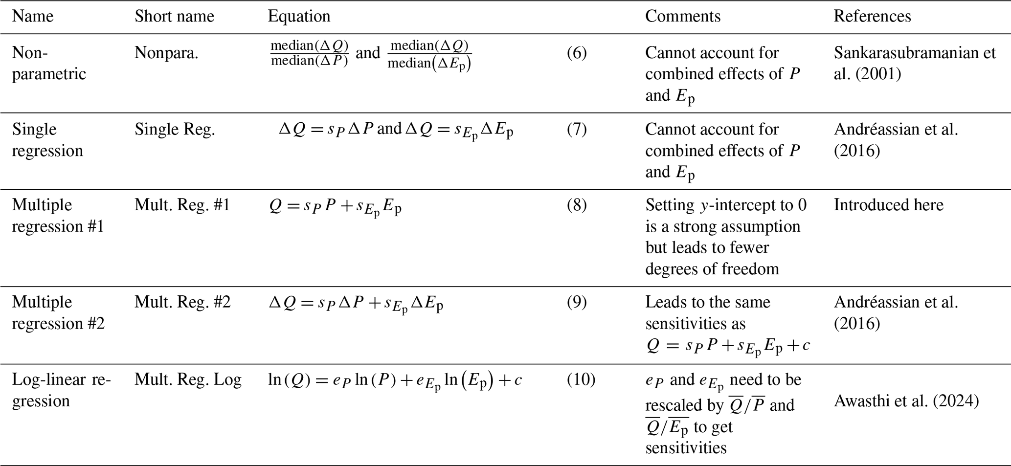
We test several methods to calculate sensitivities empirically, all listed in Table 1. In addition to the commonly used non-parametric method (Eq. 6; Sankarasubramanian et al., 2001), we use different regression-based methods (Andréassian et al., 2016). These include single linear regression using annual variations around the mean (Eq. 7), multiple linear regression using absolute annual values with y-intercept set to 0 (multiple regression #1; Eq. 8), multiple linear regression using annual variations around the mean with y-intercept set to 0 (multiple regression #2; Eq. 9), and log-linear regression (Eq. 10), which was recently proposed by Awasthi et al. (2024). We note that multiple regression #1 is not commonly used, but is included here as it yields interesting results (shown later). In addition to the regression coefficients, which represent the sensitivities, we also calculate R² to check how much variance is explained by the different regression models and to investigate if the unexplained variance shows any patterns in relation to the sensitivity estimates, as well as p-values for each fitted parameter.

Table 1 Methods used to empirically estimate streamflow sensitivity to precipitation and potential evaporation.

Besides deciding on the equation to fit (e.g., single or multiple regression), we need to decide on the fitting method when applying regression analysis (e.g., ordinary least squares or more advanced methods). Earlier studies found that the fitting method has little influence on sensitivity estimates (Andréassian et al., 2016). We also briefly tested different methods such as lasso or ridge regression (e.g., Dormann et al., 2013) and performed multiple regression sequentially (so-called stepwise partial regression), but found this to lead to virtually identical results. We thus do not further investigate the influence of the fitting method and also do not report any results here.

All methods are applied to annually averaged values. Since averaging of variables over more than a year has also been suggested (Andréassian et al., 2016; Zhang et al., 2022), we briefly tested this approach on the observational dataset and estimated sensitivities using averages over non-overlapping 5-year blocks (see Fig. S1 in the Supplement). Since this method did not lead to any obvious improvements or additional insights, we do not further discuss it here.

2.3 Analytical model of streamflow sensitivity and synthetic dataset

The Turc–Mezentsev model is a Budyko-type model that takes long-term average precipitation P, potential evaporation E_p, and a shape parameter n as input, and returns streamflow Q (and, complementary to that, actual evaporation E_a). The parameter n is often set between 2 and 3 (see e.g., Lebecherel et al., 2013) and is assumed to relate to other factors influencing the catchment water balance, such as vegetation cover (e.g., Zhang et al., 2001). While the exact value of n is not of major importance here, we use a value of n=2.2, chosen to fit our observational dataset (described in Sect. 3) best by minimizing the average absolute error (see Fig. S3 in the Supplement).

The Turc–Mezentsev model can also be used to analytically calculate the sensitivity of Q to P and E_p (which may be summarised to the aridity index $E_{\mathrm{p}}/P$) by calculating partial derivates, so that we obtain a single sensitivity curve, which is a function of the aridity index. The resulting curves for $Q/P$ (as a reference), s_P, and $s_{E_{\mathrm{p}}}$ are shown in Fig. 1.

$$\begin{array}{}\text{(11)}& {\displaystyle \frac{Q}{P}}=\mathrm{1}-{\displaystyle \frac{{\left(P^{-n}+E_{\mathrm{p}}^{-n}\right)}^{-\frac{\mathrm{1}}{n}}}{P}}\text{(12)}& {\displaystyle \frac{\partial Q}{\partial P}}=s_P=\mathrm{1}-{\left(\mathrm{1}+{\left({\displaystyle \frac{P}{E_{\mathrm{p}}}}\right)}^n\right)}^{-\frac{n+\mathrm{1}}{n}}\text{(13)}& {\displaystyle \frac{\partial Q}{\partial E_{\mathrm{p}}}}=s_{E_{\mathrm{p}}}=-{\left(\mathrm{1}+{\left({\displaystyle \frac{E_{\mathrm{p}}}{P}}\right)}^n\right)}^{-\frac{n+\mathrm{1}}{n}}\end{array}$$

Equation (11) is usually applied at long time scales, for which changes in storage are negligible (so that $P=Q+E_{\mathrm{a}}$). Accordingly, also the sensitivities (Eqs. 12 and 13) should be seen as sensitivities to long-term changes P and E_p. Here, we relax this assumption and use these equations to study year-to-year variability. We note that the same assumption is (implicitly) made in many sensitivity studies, which use year-to-year variability to estimate how catchments respond to long-term change, even though there is evidence that year-to-year variability in Q also responds to changes in, for instance, storage (Tang et al., 2020). For the theoretical analysis carried out here this does not matter, as we test how well different methods can estimate sensitivities from synthetically generated data with the assumption that storage changes are zero. It will, however, matter when interpreting sensitivity estimates based on observational data. Here, a mismatch in time scales (i.e., annual variations used to calculate empirical sensitivities vs. spatial variations of long-term water balances between catchments underlying the Turc–Mezentsev model) might lead to differences between the empirical and theoretical sensitivities.

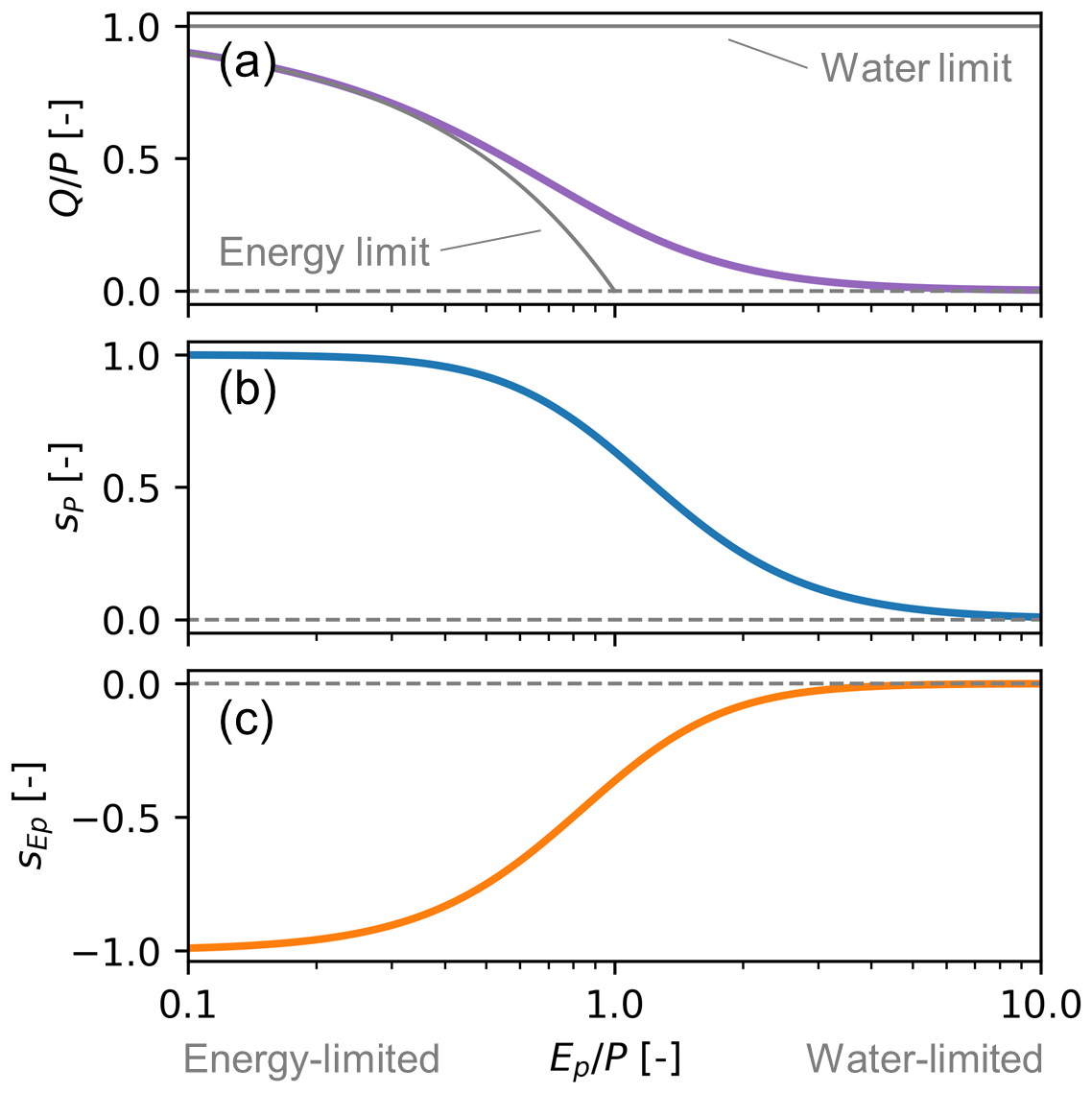
Figure 1 (a) Streamflow fraction of precipitation ($Q/P$), (b) streamflow sensitivity to precipitation s_P, and (c) streamflow sensitivity to potential evaporation $s_{E_{\mathrm{p}}}$ as a function of the aridity index ($E_{\mathrm{p}}/P$), all based on the Turc–Mezentsev model using n=2.2 (Eqs. 11–13). The grey lines in panel (a) indicate the water and energy limits, respectively. The energy limit poses a lower limit to streamflow, because not more precipitation can be lost to evaporation than potential evaporation. The water limit poses an upper limit to streamflow, because streamflow cannot exceed precipitation.

In addition, since the Turc–Mezentsev model is nonlinear, a linear regression might not match well the local derivative at the long-term mean, especially if year-to-year variability is large. To get an idea regarding how nonlinear the relationship could be for typical ranges of variability, we had a closer look at some example catchments, both synthetic ones and real ones (shown in Figs. S16 and S17 in the Supplement). The bivariate relationships between Q and P and E_p, respectively, appear to be mostly linear, though some weak nonlinearity can be seen especially for strongly water-limited catchments.

Based on the Turc–Mezentsev model, we create a synthetic dataset for which the actual sensitivities are known, which will serve as a baseline for the theoretical analysis that will follow. To do so, we first generate synthetic catchments with fixed long-term values of P and E_p that span a wide aridity gradient (both P and E_p range from 300 to 3000 mm yr⁻¹). For each synthetic catchment, we then create 50 annual value pairs by sampling from a bivariate normal distribution with the standard deviations of P and E_p set to 15 % and 5 % of their means, respectively, and with a Pearson correlation ρ_P between P and E_p set to three different values: −0.5, 0, and +0.5. The standard deviations are chosen to be similar to the ones found in the observational dataset used (17 % for P and 4 % for E_p; data are described in Sect. 3). The correlation is added because P and E_p are regularly correlated in empirical data (${\mathit{\rho }}_P=-\mathrm{0.42}$ on average for the catchments used here; see Fig. S4 in the Supplement) and this is known to affect sensitivity estimates (e.g., Chiew et al., 2014). Note that we use Pearson correlation ρ_P for the generation of correlated data, but in all other cases we use the more robust Spearman rank correlation ρ_S to quantify the strength of variable associations. Having created synthetic P and E_p data, we use the Turc–Mezentsev model to calculate Q for each annual pair of P and E_p (Eq. 11) as well as the sensitivities corresponding to the long-term values of P and E_p (Eqs. 12 and 13).

In addition, we investigate the influence of data uncertainty, which affects every hydrological variable (McMillan et al., 2012, 2018). To do so, we added normally distributed noise to P, E_p, and Q (after they have been generated). We use 2.5 % of each variable's mean as standard deviation, so that about 95 % of the data will fall within ±5 % of the mean (±2 times the standard deviation). While observational uncertainty is often estimated to be around 10 % or higher, especially for precipitation (McMillan et al., 2012, 2018), these values are not directly comparable, as data uncertainty is often systematic (e.g., due to precipitation undercatch) and might be partly averaged out when using annual sums. Since the main aim here is to investigate the potential impact of data uncertainty, we decided to use a standard deviation of 2.5 %, bearing in mind that the actual impact may vary depending on the actual uncertainty of the different variables.

Overall, we obtain 6 synthetic scenarios: three different strengths of correlation, each without and with random noise. The different sensitivity estimation methods (Table 1) are then used to derive sensitivities s_est, which are compared to the actual sensitivities s_act (Eqs. 12 and 13). This is done both visually and by quantifying the relative error as $e_{\mathrm{rel}}=(s_{\mathrm{est}}-s_{\mathrm{act}})/s_{\mathrm{act}}$ [%], which is then averaged across all samples by taking the arithmetic mean.

2.4 Temporal analysis

As can be seen from Eqs. (12) and (13), the streamflow sensitivities themselves depend on the aridity index, so that (at least theoretically) a change in aridity will lead to a change in the sensitivities. We can therefore also use the analytical model to investigate how typical temporal trends found for P and E_p translate into trends in sensitivities (or elasticities) and compare these theoretically calculated trends with empirically estimated ones. To do so, we first average P, E_p, and Q from the observational datasets (described in Sect. 3) over 20-year moving blocks in a longer time series (at least 50 years), resulting in at least 30 blocks. We then calculate both theoretical sensitivities and streamflow values (using the Turc–Mezentsev model forced with P and E_p) and empirical sensitivities (using multiple regression on P, E_p, and Q) for each 20-year block. Finally, we calculate trends of theoretical and empirical sensitivities over time with the Theil-Sen trend slope estimator (Sen, 1968). In order to calculate relative trends (in %), we normalize the trends by the sensitivities calculated in the first 20-year block (i.e., at the beginning of the time series). The trend analysis is carried out separately for different subsets of observational data (described in Sect. 3), for which we use an independently calibrated an n-value each to ensure that the Turc–Mezentsev captures regional conditions reasonably well.

2.5 Calculation of additional catchment indices

To aid catchment selection and the interpretation of the results, we calculate three further indices per catchment: a precipitation seasonality index (P_S), the fraction of precipitation falling as snow (f_S), and a baseflow index (BFI). The seasonality index quantifies the seasonal timing of precipitation relative to temperature (Woods, 2009), indicating whether most precipitation falls in summer (P_S>0) or in winter (P_S<0). The fraction of precipitation falling as snow is calculated by dividing the sum of precipitation falling on days with temperatures T below 0 °C by the total precipitation sum, and it ranges from 0 to 1. The baseflow index is a measure of how flashy or smooth a streamflow hydrograph is, often linked to groundwater contributions to streamflow. The baseflow index is calculated by dividing baseflow estimated using a digital filter (Institute of Hydrology, 1980) by total streamflow, and it ranges from 0 to 1.

Table 2 Datasets used in the study and some of their characteristics. WY denotes the start of the water year (for Germany, October is used instead of November for consistency).

3 Data

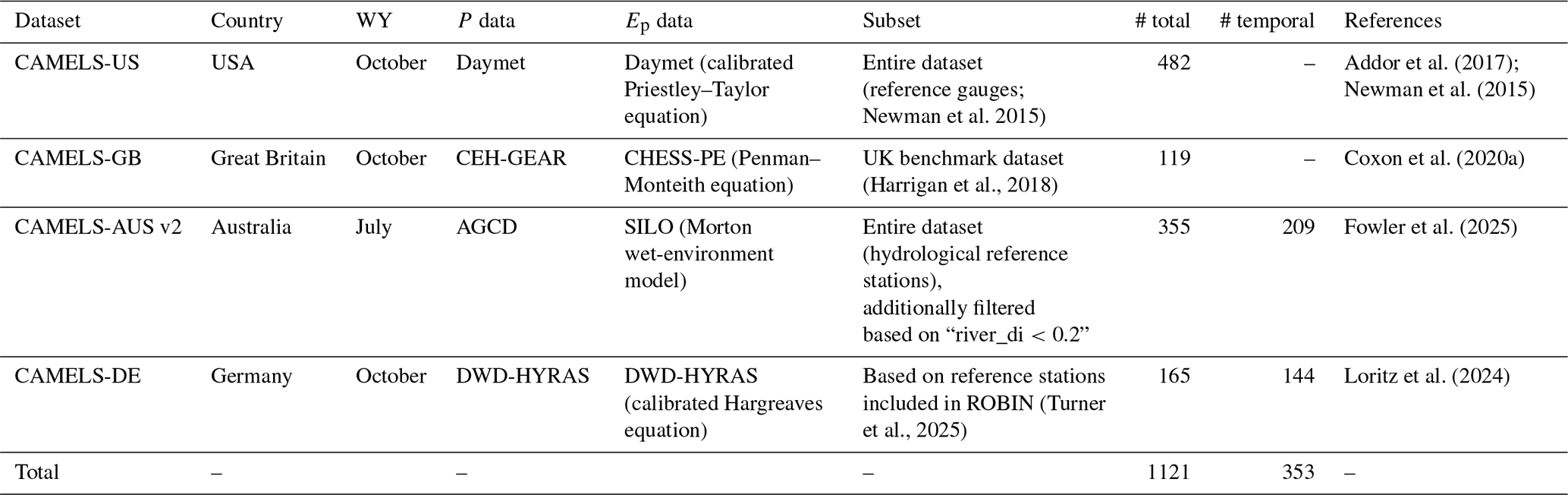
In addition to synthetic data, we also test different sensitivity estimation methods using observational data. We use data from four large sample datasets (CAMELS-US, CAMELS-GB, CAMELS-AUS v2, CAMELS-DE) and select catchments based on the following criteria: we only keep time series with less than 5 % missing values, at least 30 years in length, a fraction of precipitation falling as snow f_S<0.2, and where Q does not exceed P. All the time series are aggregated to annual values based on the water year. For the trend analysis, we focus on CAMELS-AUS and CAMELS-DE due to availability of long time series and only kept catchments with at least 50 years of data. The Australian dataset is further divided into two subsets, one where most precipitation falls in winter (P_S<0) and one where most precipitation falls in summer (P_S>0), to study trends across regions that are climatologically not too different. Details and references are reported in Table 2.

We always use national forcing products to ensure high quality data, as global products were reported to be associated with substantial uncertainties for CAMELS-US and CAMELS-GB (Clerc-Schwarzenbach et al., 2024), and as we assume that national datasets reflect regional conditions best. This come at the cost of potentially reducing comparability, though, especially regarding E_p, which is estimated using different equations (see Table 2). We therefore made a brief comparison to study the influence of different P and E_p datasets on the resulting sensitivities for CAMELS-AUS and CAMELS-DE, the two datasets used for the trend analysis. In particular, we estimated the sensitivities using P and E_p from national data sources (our default option here; see Table 2) and from their Caravan extension (Kratzert et al., 2023), which is based on ERA5-land and uses the Penman–Monteith equation in its updated version to calculate E_p (Kratzert et al., 2025).

Overall, the estimated sensitivities are similar (see also Fig. S2 in the Supplement). For CAMELS-AUS v2, we obtain a Spearman rank correlation of ρ_S=0.97 and a mean absolute error of MAE = 0.09 for streamflow sensitivity to precipitation, and ρ_S=0.94 and MAE = 0.07 for streamflow sensitivity to potential evaporation. For CAMELS-DE, we obtain ρ_S=0.94 and MAE = 0.08 for streamflow sensitivity to precipitation, and ρ_S=0.86 and MAE = 0.09 for streamflow sensitivity to potential evaporation. In conclusion, we find that the resulting sensitivities somewhat depend on the forcing products used, but that the differences are rather small and also do not substantially alter the trend analysis (not shown here). We will come back to the issue of reliably estimating E_p in the discussion, but note that this is not our main focus here.

4 Results

4.1 Comparison of sensitivity estimation methods using the analytical model

The analytical Turc–Mezentsev model allows us to test the different sensitivity estimation methods (Table 1) and compare them to theoretical values, thereby illustrating how the methods perform under known conditions. Figures 2 and 3 show the resulting sensitivity estimates for all methods as a function of the aridity index. Table 3 lists the relative errors, which are also visualised as bar plot in Fig. S5 in the Supplement.

Table 3 Relative errors e_rel [%], rounded to full percentages, and absolute average of the relative errors for the different estimation methods. Figure S5 in Supplement also shows the values as bar plots.

Figure 2 Streamflow sensitivity to precipitation as a function of the aridity index. Theoretical values are based on the Turc–Mezentsev model (n=2.2), forced with precipitation and potential evaporation values that exhibit different degrees of correlation and noise to simulate real observations. The estimates resulting from the different methods are shown as point clouds with a LOESS regression (the fraction of data points which influence the smoothing at each value is set to 0.1) to aid visualization.

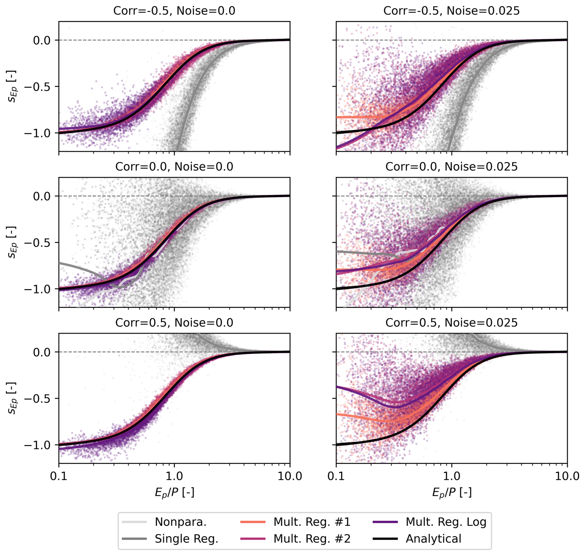
Figure 3 Streamflow sensitivity to potential evaporation as a function of the aridity index. Theoretical values are based on the Turc–Mezentsev model (n=2.2), forced with precipitation and potential evaporation values that exhibit different degrees of correlation and noise to simulate real observations. The estimates resulting from the different methods are shown as point clouds with a LOESS regression (the fraction of data points which influence the smoothing at each value is set to 0.1) to aid visualization.

Overall, the estimation of streamflow sensitivities to potential evaporation $s_{E_{\mathrm{p}}}$ results in much larger relative errors than for sensitivities to precipitations_P. The smallest relative errors are obtained in absence of noise and with no correlation between P and E_p (e_rel from −2 % to 5 %). In presence of noise, the performance degrades for most methods, especially for $s_{E_{\mathrm{p}}}$. For s_P, multiple regression methods #1 and #2 lead to the lowest relative errors overall (average absolute e_rel=2 %), followed by log-regression (4 %). For $s_{E_{\mathrm{p}}}$, multiple regression method #1 leads to the lowest relative error overall (average absolute e_rel=6 %), followed by method #2 and log-regression (both 12 %).

When P and E_p are correlated, the nonparametric method and single regression (i.e., methods that do not account for both P and E_p) lead to large and systematic errors. For instance, with negative correlations of −0.5, streamflow sensitivities to precipitation (e_rel from 6 to 10 %) and to potential evaporation (e_rel from 231 % to 314 %) are – on average – systematically overestimated (Table 3). By contrast, when correlations are set to +0.5, s_P (e_rel from −12 % to −10 %) and $s_{E_{\mathrm{p}}}$ (e_rel from −311 to −266 %) are systematically underestimated. For multivariate methods, the relative errors are much smaller, but we still find systematic errors, especially for $s_{E_{\mathrm{p}}}$ and in presence of noise. For instance, with negative correlations of −0.5 and with noise, method #1 underestimates $s_{E_{\mathrm{p}}}$ by −7 %, while method #2 and log-regression both underestimate it by −14 % (see also Fig. 3). Yet even when P and E_p are not correlated, we find systematic underestimation of $s_{E_{\mathrm{p}}}$ (e_rel from −9 % to −19 %).

4.2 Comparison of sensitivity estimation methods using observational data

Since the Turc–Mezentsev model is a very simplified representation of reality, methods that perform well compared to the theoretical values may not perform well based on observational data that are influenced by more than just P and E_p (e.g., storage changes from year to year) and that are subject to other types of uncertainty (e.g., systematic bias). Hence, we now apply two selected methods to a large sample of near-natural catchments. We decided to focus only on methods #1 and #2, since log-regression leads to very similar results as method #2 and all univariate methods lead to poor performance if P and E_p are correlated (see Figs. 2 and 3). This is indeed the case for most catchments, with Pearson correlation ρ_P between P and E_p in the observational data being mostly negative and averaging −0.42.

When applying methods #1 and #2 to observational data, we find good agreement between the two methods for s_P (Spearman rank correlation ρ_S=0.96) and little agreement for $s_{E_{\mathrm{p}}}$ (ρ_S=0.07), shown in Fig. 4. Theoretically, we would expect s_P to range from 0 to 1 and $s_{E_{\mathrm{p}}}$ to range from −1 to 0. That is, $s_{E_{\mathrm{p}}}$ should always be negative, as an increase in evaporative demand should be related to a decrease in streamflow. However, we find that 52 % of values for $s_{E_{\mathrm{p}}}$ are positive when using method #2, while it is only 3 % when using method #1. In terms of explained variance by the multiple regression methods, the two methods perform similarly. The overall median R² is 0.65 for #1 and 0.68 for #2, indicating an acceptable fit but also substantial variation left unexplained. The p-values, shown in Fig. S10 in the Supplement, are almost always larger than 0.05 for s_P (in more than 99 % of the catchments). The p-values for $s_{E_{\mathrm{p}}}$ vary, with values being smaller than 0.05 in 83 % of the catchments for method #1 and only in 16 % of the catchments for method #2.

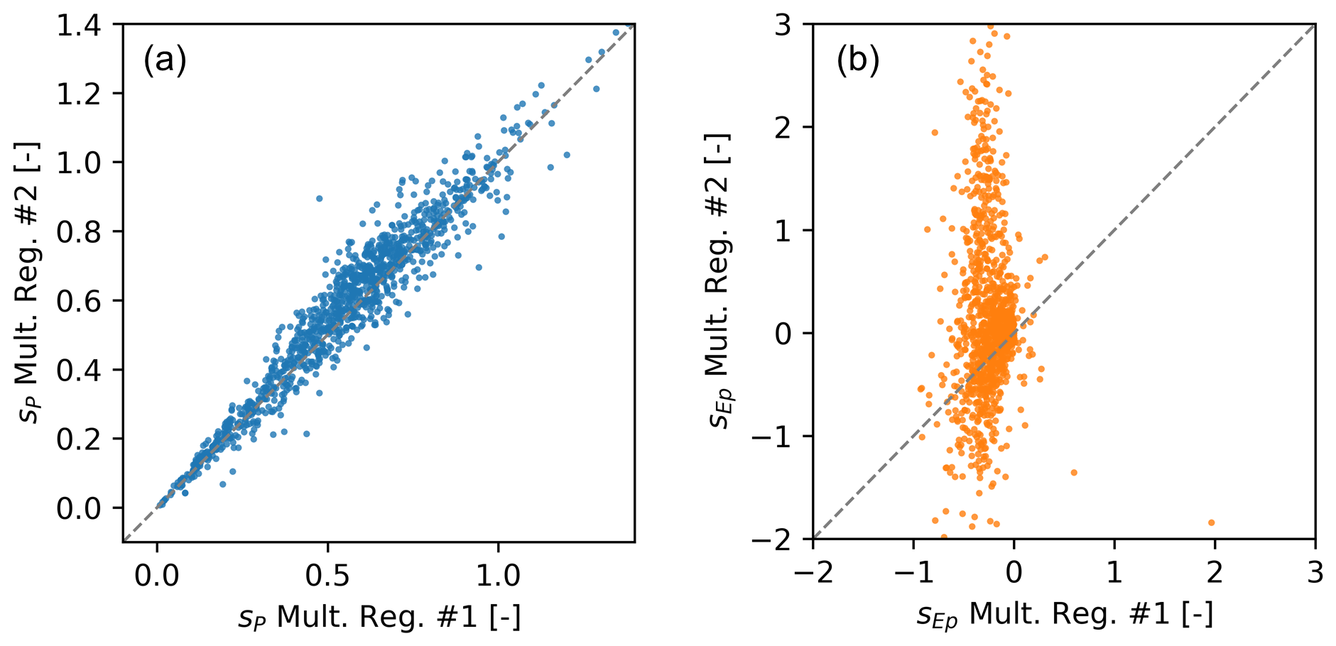
Figure 4 Comparison of streamflow sensitivity to (a) precipitation (ρ_S=0.96) and (b) potential evaporation (ρ_S=0.07) calculated using multiple regression methods #1 and #2 with observations from 1121 catchments. The grey dashed line shows the 1:1 line.

Since there is little difference for s_P and method #1 provides the most realistic values for $s_{E_{\mathrm{p}}}$, the following analyses are based on method #1. We also added all figures using method #2 to the Supporting Information. We first compare the empirically estimated sensitivities to the Turc–Mezentsev model, shown in Fig. 5. Overall, both s_P and $s_{E_{\mathrm{p}}}$ follow the theoretical pattern and decrease with increasing aridity (the results are similar for elasticities; see Fig. S6 in the Supplement).

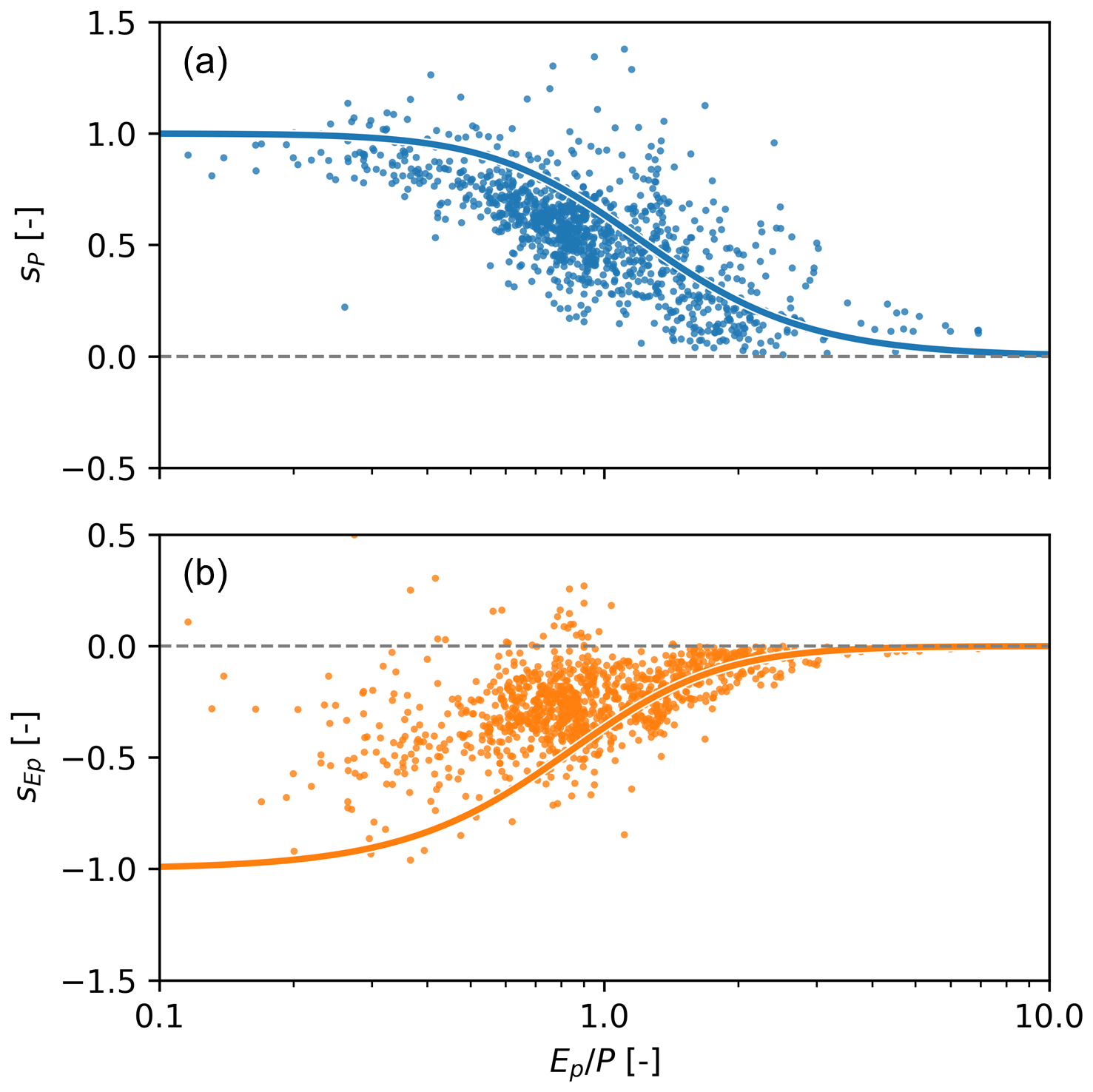
Figure 5 Streamflow sensitivity to (a) precipitation and (b) potential evaporation, calculated using multiple regression #1 with observations from 1121 catchments. Both panels show empirically calculated values (dots) and theoretical values based on the Turc–Mezentsev model with n=2.2 (solid lines). Note that the y-axes are capped for better visibility and that two catchments plot above 0.5 for $s_{E_{\mathrm{p}}}$.

The fact that the sensitivities estimated empirically using year-to-year variability show a similar pattern as the sensitivities obtained by calculating partial derivates of a spatial relationship (Eqs. 12 and 13) hints at some degree of space-time-symmetry. However, the theoretical values tend to be underestimated and there is substantial variability, clearly more than for a Budyko-type plot of the same catchments (shown in Fig. S3 in the Supplement). The R² values tend to be smaller for catchments further away from the theoretical Turc–Mezentsev curves (using n=2.2), with ρ_S between R² and the relative deviation of the empirical sensitivities from the Turc–Mezentsev curve being 0.60 for s_P and 0.25 for $s_{E_{\mathrm{p}}}$ (see Fig. S11 in the Supplement). This suggests that other predictors not included in the regression model matter, too.

We briefly considered several other factors commonly hypothesised to influence annual Q variability apart from P and E_p, namely storage, seasonality, and snow, here approximated with BFI, P_S, and f_S, respectively. In particular, we tested if the differences between the Turc–Mezentsev-based sensitivities (i.e., the curves shown in Fig. 5) and the empirical sensitivities are related to any of these variables (see also Figs. S12–S14 in the Supplement). We found the strongest correlation between the relative deviation from the Turc–Mezentsev curve and BFI (${\mathit{\rho }}_{\mathrm{S}}=-\mathrm{0.41}$ for s_P and −0.44 for $s_{E_{\mathrm{p}}}$), followed by f_S (−0.31 and −0.46), and P_S (0.09 and 0.20).

Another way to visualise the resulting sensitivities is to plot s_P and $s_{E_{\mathrm{p}}}$ against each other, which is shown in Fig. 6 with each catchment coloured according to its aridity index. We can see that the Turc–Mezentsev model leads to a single curve, meaning that each s_P is associated with a unique $s_{E_{\mathrm{p}}}$, both being a function of the aridity index (cf. Eqs. 12 and 13). The same holds true for elasticities e_P and $e_{E_{\mathrm{p}}}$, which plot as a straight line that follows the so-called complementary relationship ($e_P+e_{E_{\mathrm{p}}}=\mathrm{1}$). The empirical patterns roughly follow the analytical ones in the case of sensitivities, and almost show a perfect match for elasticities. Note, though, that this refers to the overall pattern and not individual catchments, which may sit on the theoretical line but at the wrong location with respect to their aridity index.

Figure 6 (a) Streamflow sensitivity to precipitation plotted against streamflow sensitivity to potential evaporation. (b) Streamflow elasticity to precipitation plotted against streamflow elasticity to potential evaporation. Both panels show empirically calculated values using multiple regression #1 (dots in the back) and theoretical values based on the Turc–Mezentsev model (line in front), coloured according to the aridity index. The grey dashed line starts at the origin and has a slope of −1, so that values plotting above it imply that $s_P\mathit{>}{s}_{E_{\mathrm{p}}}$ (a) and $e_P\mathit{>}{e}_{E_{\mathrm{p}}}$ (b).

4.3 Change of sensitivities over time

The strong relationship between streamflow sensitivity and aridity index found when comparing many catchments (Fig. 5; Andréassian et al., 2025a; Sankarasubramanian et al., 2001) suggests that a change in aridity index over time will also lead to changes in sensitivities for individual catchments. Theoretically, the Turc–Mezentsev model predicts a decrease (in absolute terms) in both sensitivities as aridity increases. Using sufficiently long observational records, we can calculate actual trends using sensitivity estimates over different time blocks (here based on method #1) and compare them to theoretical trends (via Eqs. 12 and 13) based on observed changes in precipitation and potential evaporation (and thus aridity index). This is done separately for Germany and two Australian subsets, which were split according to whether most precipitation falls in winter or in summer. The resulting trends are shown in Figs. 7 and quantified in Table S1 in the Supplement. We find an increase in the aridity index over time, especially in Germany. Accordingly, the sensitivities decrease (in absolute terms) over time in all cases. However, the trend magnitudes are overall stronger in observational data (between 15 % and 70 % decrease) than in the analytical model (between 5 % and 26 % decrease). In Germany, we generally find lower sensitivities than based on the Turc–Mezentsev model, but the trends in the observational data are larger (26 % vs. 5 % for s_P and 70 % vs. 11 % for $s_{E_{\mathrm{p}}}$), see Fig. 7a. In the Australian subset where most precipitation falls in winter, we find a somewhat similar pattern, with larger trends in the observational data than in the model (40 % vs. 18 % for s_P and 49 % vs. 26 % for $s_{E_{\mathrm{p}}}$), see Fig. 7b. In the Australian subset where most precipitation falls in summer, both the sensitivities and the trends are relatively close to the analytical model (15 % vs. 8 % for s_P and 15 % vs. 15 % for $s_{E_{\mathrm{p}}}$), see Fig. 7c.

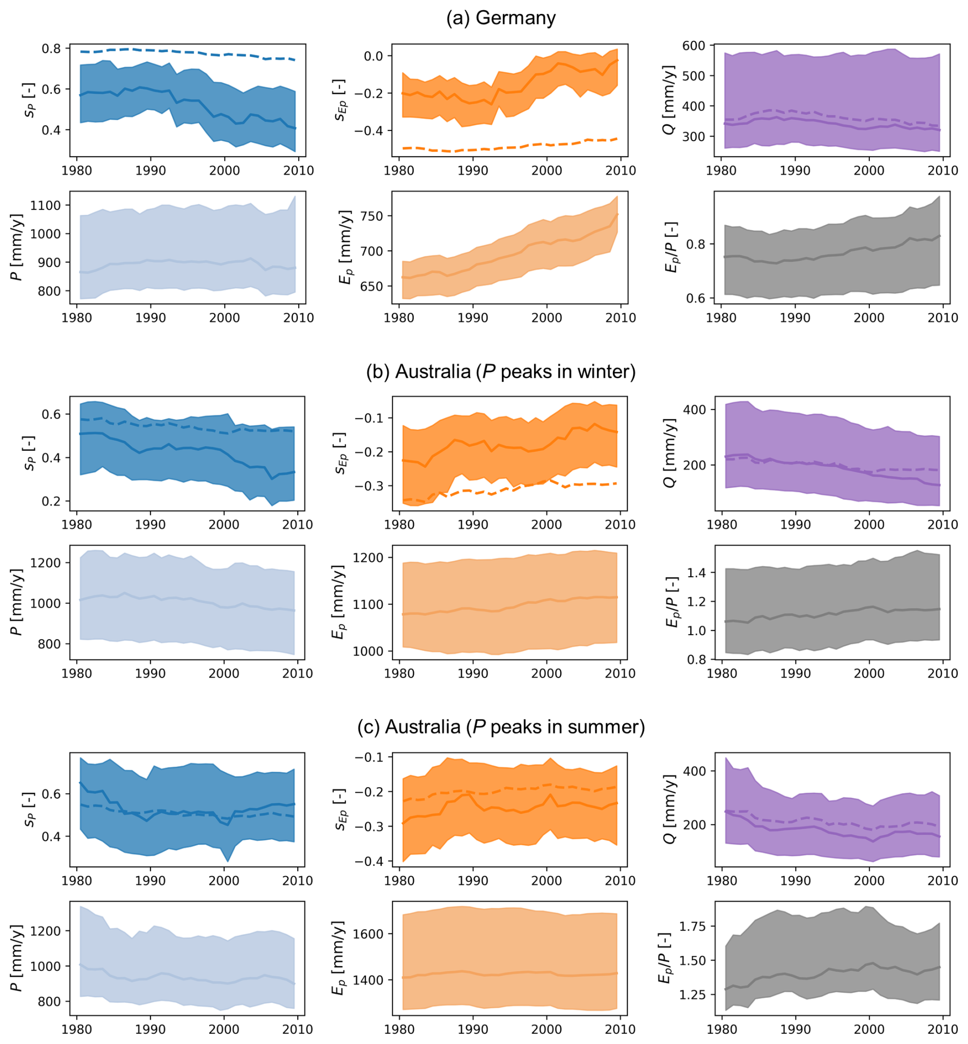
Figure 7 Change of streamflow sensitivities and other variables over time for (a) 144 catchments in Germany, (b) 100 catchments in Australia with most precipitation falling in winter (P_S<0), and (c) 109 catchments in Australia with most precipitation falling in summer (P_S>0). Shaded areas indicate the 25th and 75th percentiles and thick lines indicate the median of all catchments. Dashed lines indicate the trends calculated with the Turc–Mezentsev model for the sensitivities and Q based on observed P and E_p data and using a calibrated value of n=1.9 for (a), n=1.7 for (b) and n=2.6 for (c). Sensitivities are calculated using method #1 over 20-year blocks with the middle year shown (e.g., 1980 indicates a block from 1970 to 1990).

In absolute terms, most of the observed trends are in the order of around 0.15, meaning that at the end of the 50-year period a catchment that originally experienced a decrease of 0.5 mm in Q per mm decrease in P would now experience a decrease of only 0.35 mm in Q per mm decrease in P. Conversely, an increase in E_p at the end of the time period would lead to a smaller absolute reduction in Q, even though E_p related trends are likely less reliable given the uncertainty discussed previously.

5 Discussion

5.1 Comparison of sensitivity estimation methods using an analytical model

Overall, univariate methods are unreliable in presence of correlation between P and E_p, which is the case for most catchments studied here (average ${\mathit{\rho }}_P=-\mathrm{0.42}$). While the limitation of univariate methods has been reported before (e.g., Andréassian et al., 2016), our results explicitly link errors in univariate methods to the correlation between P and E_p. The nonparametric method and single regression are therefore unreliable sensitivity estimators in most cases, especially for of $s_{E_{\mathrm{p}}}$. In addition, even multivariate methods show systematic deviations from the analytical curves. While the multivariate methods always lead to an underestimation of $s_{E_{\mathrm{p}}}$ (i.e., less negative values) in presence of noise, the curves shown in Fig. 3 still tend to be more negative on average for ${\mathit{\rho }}_P=-\mathrm{0.5}$ and more positive on average for ${\mathit{\rho }}_P=+\mathrm{0.5}$, which is the same general pattern as for the univariate methods. It is sometimes argued that multiple regression accounts for the correlation between predictors, yet this statement may be a bit misleading. Multiple regression estimates the effect of one predictor while holding the others constant, but strong correlations between predictors (multicollinearity) can inflate standard errors and produce poorly conditioned coefficients that are highly sensitive to small changes in the data (Dormann et al., 2013). In presence of strong correlations (e.g., when wet years are typically associated with reduced potential evaporation), there is little variation in one predictor that does not overlap with the other, making it difficult to estimate unique effects.

Multivariate methods perform relatively reliable for s_P (2 %–5 % relative error on average), but they are less reliable for $s_{E_{\mathrm{p}}}$ (6 %–12 % relative error on average). The absolute values of $s_{E_{\mathrm{p}}}$ are always smaller than for s_P for a given aridity index (see e.g., Fig. 7a, where all theoretical values plot above the dashed line) and so is their year-to-year variability (standard deviation was set to 15 % for P and 5 % for E_p), which could explain why $s_{E_{\mathrm{p}}}$ is generally more difficult to estimate. This is substantiated by two additional checks (not shown here): if we increase the noise (smaller signal-to-noise ratio), the relative errors for both s_P and $s_{E_{\mathrm{p}}}$ increase; and if we increase the year-to-year variability of E_p in comparison to P, the relative errors for s_P and $s_{E_{\mathrm{p}}}$ become higher and lower, respectively.

Overall, the general underestimation (in absolute terms) of $s_{E_{\mathrm{p}}}$ in presence of noise might thus largely be due to relatively little variation in E_p compared to P and to noise (cf. regression dilution), with additional bias due to correlation between P and E_p. While there are other regression methods that could be tested, our results suggest that the problem lies not primarily in the fitting method, but rather in general limitations of using (multiple) regression to estimate sensitivities from noisy and correlated data. In summary, despite the simplicity of our synthetic experiment, it illustrates that none of the methods can reliably estimate the sensitivities in all cases. This suggests similar or larger uncertainties for observational data, where additional factors may complicate the estimation of sensitivities, such as systematic biases (e.g., due to precipitation undercatch) or water balance issues (e.g., due to inter-catchment groundwater flow). This could also be studied using a synthetic experiment, but is beyond the scope of this paper.

5.2 Comparison of sensitivity estimation methods using observational data

5.2.1 Uncertainty in empirical sensitivity estimates

Overall, multiple regression methods #1 and #2 lead to similar values for s_P, but show large disagreement for $s_{E_{\mathrm{p}}}$. This generally agrees with the results using the analytical model, which also showed larger disagreement for $s_{E_{\mathrm{p}}}$. As discussed in Sect. 5.1, absolute values of $s_{E_{\mathrm{p}}}$ are always smaller than for s_P, and previous studies also reported that changes in precipitation dominate the streamflow response of catchments (Berghuijs et al., 2017; Zhang et al., 2023). In addition, year-to-year variability in E_p (standard deviation of 4 % on average) tends to be smaller than for P (17 %), so that the already smaller $s_{E_{\mathrm{p}}}$ might be more difficult to constrain empirically, since the signal-to-noise ratio is relatively low (cf. Chiew et al., 2014). Alternative options which may help to constrain sensitivity values through regionalisation are pooled regression methods (e.g., panel regression; Anderson et al., 2025; Awasthi et al., 2024). This may allow robust estimation at the regional scale, although at the expense of unreliable sensitivity estimates at individual locations.

More than half of the values based on method #2 are larger than zero, which would suggest an increase in streamflow with increasing E_p. This cannot be generally attributed to concurrent increases in P, because P and E_p are anti-correlated. A considerable fraction of positive or zero values for sensitivities (or elasticities) to potential evaporation or temperature was also reported in other papers (Anderson et al., 2022; Andréassian et al., 2016, 2025b; Awasthi et al., 2024; Xiao et al., 2020; Zhang et al., 2023). While this may be perceivable in certain circumstances (e.g., when warmer years are associated with increased precipitation intensity, or due to melt water contributions) it is unrealistic for this to occur in more than half of all catchments, casting doubt on the reliability of these sensitivity estimates. Alternatively, if these sensitivities were to capture actual catchment behaviour, it would imply that both simple Budyko-type and more complex simulation models, which usually show negative sensitivities to E_p (e.g., Roderick and Farquhar, 2011; Xiao et al., 2020), omit or misrepresent crucial processes related to evaporation. While method #1 leads to values of $s_{E_{\mathrm{p}}}$ that mostly fall between −1 and 0, these values are often relatively small compared to the Turc–Mezentsev model. This might partly be a consequence of the method, which showed systematic underestimation in the synthetic experiment (Fig. 3). Hence, these $s_{E_{\mathrm{p}}}$ estimates should also be interpreted with caution.

5.2.2 Patterns in empirical streamflow sensitivities and influence of catchment storage processes

Comparing observation-based sensitivities to the Turc–Mezentsev model, we find that both s_P and $s_{E_{\mathrm{p}}}$ tend to be lower in observational data. Since Turc–Mezentsev is a climate-only model, actual sensitivities to climate (P and E_p) are lower in real catchments where other factors matter, too. Besides data uncertainty, these include storage processes, seasonality, snow, vegetation characteristics, or inter-catchment groundwater flow (e.g., Andréassian et al., 2025b; Weiler et al., 2025; Zhang et al., 2023). It is also likely that in less strictly filtered catchment datasets (see Sect. 2.5), the scatter will be larger due to other influences, such as human interventions in the water cycle. Still, especially s_P follows the theoretical pattern relatively well, substantiating the strong influence of the aridity index on streamflow sensitivities.

The catchments that fall further away from the Turc–Mezentsev curves tend to have lower R² and correlate substantially with the BFI and the snow fraction, and only weakly with precipitation seasonality. This can only be viewed as a very preliminary analysis, because other (more difficult to calculate) factors could have also been tested and because these different factors are not completely independent of each other. Still, they suggest that catchments with high BFI and large snow fractions tend to have lower sensitivities, possibly because these processes buffer year-to-year variability in precipitation and potential evaporation. While precipitation seasonality was shown to influence streamflow sensitivities in other studies (Andréassian et al., 2025b; Sankarasubramanian et al., 2001), this effect was less clearly pronounced here.

Though our main focus here is not to investigate in detail additional influences on sensitivities, we also fitted a regression model that includes a storage term, here approximated by the average streamflow from the previous year (see Fig. S15 in the Supplement). This led to two main insights. First, the median R² increased from 0.65 to 0.69, suggesting that the storage term adds some, but not much, explained variance. Second, s_P and $s_{E_{\mathrm{p}}}$ stayed almost the same, indicating that the storage term only explains additional variance not captured by the other sensitivities, and does not change their values. While additional variables can therefore be included in the sensitivity calculation, it is worth noting that (unlike here) this could lead to changes in the sensitivity estimates. If the sensitivities depend on the regression model fitted, interpretation of the resulting regression coefficients becomes more challenging. Also, regression models with many predictors increase the risk of overfitting (e.g., to certain combinations of catchments with specific correlation structures), especially when predictors are correlated or the signal-to-noise ratio is low. Thus, while including additional variables may increase our understanding of the drivers of (annual) streamflow variations (e.g., Andréassian et al., 2025b), it also necessitates a close look at the meaning and robustness of the resulting sensitivity estimates.

5.2.3 The complementary relationship

Interestingly, method #1 appears to enforce the so-called complementary relationship (Awasthi et al., 2024; Dooge, 1992; Zhou et al., 2015). This might be due to the nature of the equation used. If we reformulate Eq. (8) and substitute the sensitivities with elasticities, we get:

$$\begin{array}{c}{\displaystyle }Q=s_{P}P+s_{E_{\mathrm{p}}}{E}_{\mathrm{p}}=e_P{\displaystyle \frac{\stackrel{\mathrm{‾}}{Q}}{\stackrel{\mathrm{‾}}{P}}}P+e_{E_{\mathrm{p}}}{\displaystyle \frac{\stackrel{\mathrm{‾}}{Q}}{{\stackrel{\mathrm{‾}}{E}}_{\mathrm{p}}}}{E}_{\mathrm{p}}\\ {\displaystyle }\begin{array}{rl}\mathrm{1}& =e_P{\displaystyle \frac{\stackrel{\mathrm{‾}}{Q}}{\stackrel{\mathrm{‾}}{P}}}{\displaystyle \frac{P}{Q}}+e_{E_{\mathrm{p}}}{\displaystyle \frac{\stackrel{\mathrm{‾}}{Q}}{{\stackrel{\mathrm{‾}}{E}}_{\mathrm{p}}}}{\displaystyle \frac{E_{\mathrm{p}}}{Q}}=e_P{\displaystyle \frac{\stackrel{\mathrm{‾}}{Q}}{\stackrel{\mathrm{‾}}{P}}}{\displaystyle \frac{(\stackrel{\mathrm{‾}}{P}+\mathrm{\Delta }P)}{(\stackrel{\mathrm{‾}}{Q}+\mathrm{\Delta }Q)}}\\ & +e_{E_{\mathrm{p}}}{\displaystyle \frac{\stackrel{\mathrm{‾}}{Q}}{{\stackrel{\mathrm{‾}}{E}}_{\mathrm{p}}}}{\displaystyle \frac{({\stackrel{\mathrm{‾}}{E}}_{\mathrm{p}}+\mathrm{\Delta }{E}_{\mathrm{p}})}{(\stackrel{\mathrm{‾}}{Q}+\mathrm{\Delta }Q)}}\end{array}\end{array}$$

If we assume that the fluctuations are much smaller than the means, the means cancel out and we get: $\mathrm{1}\approx e_P+e_{E_{\mathrm{p}}}$.

While the complementary relationship should hold if catchments follow Budyko-type behaviour (i.e., Q is solely controlled by variability in P and E_p), real catchments do not necessarily behave that way. As soon as other factors (e.g., storage, changes in vegetation, human impacts) strongly affect a catchment's water balance and/or its sensitivity, we should not expect the relationship to hold. It is worth noting that the complementary relationship may be extended to account for elasticities to any number of driving variables (cf. Zhou et al., 2015). Yet, this should only be valid if all (major) drivers of streamflow variability are accounted for and in absence of large uncertainties. Overall, the so-called complementary relationship can thus be used to constrain sensitivity estimates, but also invokes assumptions that should be stated and assessed.

5.2.4 Other uncertainties and limitations

There are various sources of uncertainty when working with observational data, which will affect empirically estimated sensitivities. Besides measurement uncertainty, catchment averages of P and E_p rely on spatial interpolation procedures that introduce uncertainty (McMillan et al., 2012, 2018). These uncertainties are typically not purely random and may affect empirically estimated sensitivities in systematic ways. For instance, systematic underestimation of P (especially its variability) will lead to lower sensitivities. But even random uncertainties can affect sensitivity estimated based on linear regression, since large uncertainties compared to natural variability (i.e., a low signal-to-noise ratio) will impact the accuracy of regression coefficients, as shown in the synthetic experiment.

To minimise uncertainties arising from observational data, we selected catchments that are relatively unimpacted and come with long, mostly complete time series. We also only used national forcing products, since they are usually less uncertain than global products (Clerc-Schwarzenbach et al., 2024). In the case of the German catchments, for instance, the Hargreaves E_p estimates contained in CAMELS-DE differ substantially from Penman–Monteith E_p estimates (ρ_S=0.38) contained in Caravan, even though this difference does not substantially affect the resulting sensitivities (see Fig. S2). The data comparison here was rather brief, however, and a more extensive comparison of different E_p estimates might provide additional insights. More generally, since E_p is not a measurable but a modelled quantity, it is also associated with substantial conceptual uncertainty. One alternative option would be the use of net radiation (normalised by latent heat of vaporisation) directly to avoid the use of a model for estimating potential evaporation, which may become even more uncertain when looking at climate projections (cf. Milly and Dunne, 2016).

5.3 Change of sensitivities over time

When investigating long time spans (50 years), we find that – in accordance with the analytical model – the sensitivities decrease as aridity increases. This finding is mirrored in results previously reported for elasticities in the US (Anderson et al., 2025), though the trends there were less clearly expressed, differed between regions, and were not explicitly related to trends in aridity. While not directly comparable, the relative trends estimated here (between 15 % and 70 % decrease) are in a similar range as the relative variations in interannual elasticity compared to long-term elasticity estimates (between 4 % and 48 %) found by Anderson et al. (2025), which also showed lower elasticity in hot and dry years. This suggests that temporal changes in sensitivities of that order of magnitude are a more widespread phenomenon. Overall, both s_P and $s_{E_{\mathrm{p}}}$ decrease substantially over the 50 years investigated, suggesting that sensitivities may not be robust metrics for mid- to long-term projections. This holds true even without considering other factors that might influence the water balance in a future with elevated CO₂ concentrations (e.g., interactions between P and E_p, or changes in stomatal conductance).

Especially for the German catchments and the Australian subset where most precipitation falls in winter (Fig. 7), the theoretical and empirical trends show large differences. For both subsets, we find that the decreasing trend is larger than predicted by the analytical model and that the sensitivities themselves are lower than the Turc–Mezentsev estimates. It is unlikely that these differences are solely due to data uncertainty, because they generally remain when different data sources are used. Rather, the results suggest that these catchments (or at least their year-to-year variations) are less driven by annual totals of precipitation and potential evaporation, for instance due to larger influence of catchment storage, precipitation seasonality, or changes in land cover and human impacts. Interestingly, the average trend in streamflow is roughly captured by Turc–Mezentsev model calibrated to each subset, but the sensitivities are not (see Fig. 7). This substantiates that year-to-year variability is, in many catchments, not necessarily a good proxy for responses to longer term climatic changes.

The influence of precipitation seasonality is not conclusive, as the pattern found for the German catchments where most precipitation falls in summer is more similar to the pattern found for the Australian subset where most precipitation falls in winter. Yet the German catchments and the Australian subset with winter dominant precipitation both have relatively high BFI values on average, much higher than the Australian subset with summer dominant precipitation (see Fig. S18). In line with the previous finding that catchments with high BFI have lower sensitivities, the same catchments might also respond less directly to climatic trends, for instance due to slower groundwater responses. Finally, while we fitted the n-value to each subset for the trend analysis, using a fixed value might also explain some of the difference between analytical and empirical trends, as it has been shown that n might change as a consequence of vegetation adapting to new conditions (Nijzink and Schymanski, 2022). These present just some hypotheses that might explain (parts of) the trends, but that require more extensive testing.

6 Conclusions

A systematic comparison of empirical, primarily regression-based, methods for estimating streamflow sensitivities to precipitation and potential evaporation indicates that streamflow sensitivity estimates are often highly uncertain, especially for potential evaporation. This applies both to a synthetic experiment using an analytical model (Turc–Mezentsev) and to observations from >1000 near-natural catchments, and can also be transferred to streamflow elasticities. While multivariate regression methods are preferable over univariate methods, the commonly employed multiple regression approach resulted in unrealistic streamflow sensitivities to potential evaporation for the majority of catchments studied here. Using a variant of multiple regression (with an intercept of zero) resulted in the lowest relative errors in the synthetic experiment and leads to fewer unrealistic values when applied to observational data, likely because it enforces the complementary relationship (which states that elasticities to P and E_p should sum up to 1). This method, however, invokes strong assumptions and may still underestimate (or poorly estimate) sensitivities to potential evaporation, and should therefore not be regarded as a definite recommendation. One possible reason for the difficulty in estimating sensitivity to potential evaporation is the low year-to-year variability in potential evaporation compared to precipitation and compared to observational uncertainty. Using unrealistic estimates of sensitivities to potential evaporation may be particularly problematic in regions where climate change impacts are largely driven by changes (typically increases) in evaporative demand and not precipitation totals, as is the case for Germany. In such instances, sensitivity-based projections may be deemed unreliable even if sensitivity to precipitation is accurately estimated. In addition, both theoretical and empirical results show that sensitivities decrease over time as aridity increases, indicating that static sensitivities may be unreliable for projections of climate change impacts. Lastly, while the sensitivities are strongly related to the aridity index, we found evidence that catchments with larger influence of storage processes (e.g., groundwater, snow) show lower sensitivities to climate variables but also stronger trends than predicted by the analytical model. Overall, our results should urge caution in the use of empirical sensitivities for both short-term and long-term projections and highlight the need for further investigation.