Unravelling groundwater's role in soil-plant-atmosphere continuum: integrated ecohydrological modelling approach using STEMMUS-SCOPE and MODFLOW 6

Soil-plant-atmosphere continuum (SPAC) models are commonly used to investigate various components' role(s) in ecosystem functioning. Yet, in most SPAC models, groundwater is ignored or at best represented in an over-simplified manner, leading to misunderstanding of its critical role in simulating soil-vegetation dynamics. This study investigates groundwater's role in SPAC processes, in particular, the impacts of groundwater component (mass and energy) on: (1) regulating the soil profile, in terms of moisture and temperature; (2) the dynamics of the unsaturated/saturated zones and their further impact on water fluxes; and (3) the carbon fluxes and vegetation physiological processes (i.e. root water uptake and photosynthesis reflected by fluorescence). To address this, an integrated ecohydrological modelling (IEM) framework is developed by coupling the STEMMUS-SCOPE SPAC model with the MODFLOW 6 integrated hydrological model. The standalone STEMMUS-SCOPE (ST-SC) and the coupled STEMMUS-SCOPE-MODFLOW 6 (ST-SC-MF6) models were applied over an 8-year period (1 April 2016–31 March 2024) to three sites in the Netherlands (Loobos, Cabauw and Veenkampen). Various essential variables, including soil moisture (θ), soil temperature (T_s), groundwater level (GWL), groundwater temperature (GT), evapotranspiration (ET), gross primary productivity (GPP), net ecosystem exchange (NEE), and sun-induced chlorophyll fluorescence (SIF) were simulated and then compared to corresponding in-situ observations. Performance of both ST-SC and ST-SC-MF6 was evaluated using the Kling–Gupta efficiency (KGE) and the root mean square error (RMSE) metrics. Results indicated that the groundwater contribution is spatially and temporally variable. The ST-SC-MF6 model showed better agreement with observations than the ST-SC, improving the KGE values for: (a) θ (+0.29), T_s (+0.19), and ET (+0.35) at Loobos, (b) θ (+0.30), T_s (+0.14), NEE (+0.18), and SIF (+0.15) at Cabauw, and (c) θ (+0.21) and ET (+0.15) at Veenkampen. Notably, benefits of ST-SC-MF6 simulation were particularly prominent during both wet and dry periods, i.e. improving the representation of: (a) the θ dynamics during wet conditions, when hydraulic connectivity between the phreatic surface and the unsaturated zone is strong; (b) the root water uptake and carbon assimilation during dry periods, when shallow groundwater mitigated vegetative water stress; and (c) the T_s dynamics during both wet and dry periods, influenced by both GT and GWL, and further propagated to other T_s-dependent processes/variables such as canopy temperature. Overall, the proposed ST-SC-MF6 IEM helped to: (1) incorporate groundwater as a key component of the water, energy and carbon cycles; and (2) define the important role groundwater dynamics plays in the SPAC for deepening the understanding of ecosystem functioning.

1 Introduction

The interactions among the soil, water, vegetation and atmosphere play a fundamental role in regulating ecosystem functioning. These interactions include hydrological, thermal and carbon processes that collectively shape the dynamics of the water, energy and carbon cycles. Deepening the understanding of such interactions is crucial for better supporting ecosystem resilience against the adverse impact of climate change and anthropogenic activities (Chen et al., 2024; Dai et al., 2024). To assess and monitor ecosystem functioning, a range of different physical variables are recognized (Bojinski et al., 2014; GCOS, 2025). Examples of such variables, in particular the vegetation ones are: leaf area index, above- and below-ground biomass (Atkins et al., 2018; de Conto et al., 2024), gross primary productivity, net ecosystem exchange, evapotranspiration, plant phenology (Shi et al., 2023), and more recently the sun-induced chlorophyll fluorescence (SIF), which serves as a proxy for tracking the photosynthesis process (Sun et al., 2023). Additionally, other soil-related variables play a significant role in characterizing the ecosystem's functioning, i.e. soil moisture, surface and subsurface temperature, and evaporation (Bojinski et al., 2014; Zeng et al., 2019b; GCOS, 2025).

Soil-plant-atmosphere continuum (SPAC) models and land surface models (LSMs) are widely used to simulate most of the aforementioned variables. SPAC models simulate the transfer of thermal energy and mass (water and carbon) between soil, plants (through roots, stems and leaves), and the atmosphere (Guo, 1992). LSMs simulate the movement of energy, water, and carbon between the Earth's land surface and the atmosphere. Both model categories are often used interchangeably in the literature as they share several core physical functionalities. Furthermore, both LSMs/SPAC models are capable of assimilating remote sensing (RS) information such as canopy reflectance, vegetation optical depth, and SIF (Yang and Lei, 2024). Integrating the RS data into these models enables upscaling the simulated processes from point (plant) scale to regional scales (Senf, 2022; Van Cleemput et al., 2025), allowing for predicting ecosystem responses to regional environmental changes (Dronova and Taddeo, 2022). Examples of SPAC models are the Soil-Plant-Atmosphere (SPA) model (Williams et al., 1996, 2001), STEMMUS-SCOPE model (Wang et al., 2021) – the integration of Simultaneous Transfer of Energy, Mass, and Momentum in Unsaturated Soil (STEMMUS) and Soil Canopy Observation, Photochemistry, and Energy Fluxes (SCOPE), and the Soil Water Atmosphere Plant (SWAP) model (van Dam et al., 2008 – specifically the version coupled to the World Food Studies (WOFOST) model; de Wit et al., 2019). Examples of LSMs are the Community Land Model (CLM5; Lawrence et al., 2019), the Tethys-Chloris (T&C) model (Fatichi et al., 2012), and the Noah-MP model (Niu et al., 2011). However, the existing LSMs/SPAC models either ignore or oversimplify the underlying groundwater system by neglecting spatio-temporal variability in groundwater variables (e.g., head and temperature), and processes (e.g., recharge, discharge and groundwater evapotranspiration). Thus, the LSMs/SPAC models lack or simplify the groundwater influence on the simulated processes.

For most landscapes, groundwater storage is generally the largest component of the local water budget. It plays a vital role in sustaining essential ecosystem services by mitigating biodiversity loss and buffering against climate change (Saccò et al., 2024). Many ecosystems rely primarily on groundwater resources, so-called groundwater-dependent ecosystems, to maintain their ecological functions (Lubczynski, 2009; Kløve et al., 2014). Groundwater-dependent ecosystems can be exposed to surface water – groundwater interactions through altered recharge or discharge rates. Such changes may impair their ecological functions if groundwater availability declines, particularly under future climate regimes (Otoo et al., 2025). In other upland bedrock ecosystems, woody vegetation can even access moisture held in weathered or fractured bedrock storage (McCormick et al., 2021). Groundwater can also have a significant effect on enhancing carbon assimilation, plant growth and productivity (Ruehr et al., 2023). Under shallow water table conditions, groundwater dynamics are significant, exerting a strong influence on the soil moisture distribution and the evapotranspiration rates (Martínez-de la Torre and Miguez-Macho, 2019). Additionally, groundwater systems typically respond slower to meteorological forcing, as compared to the surface water or the near-surface soil moisture, due to their larger storage and longer flow paths. This relative hydrological stability allows groundwater to continue supporting vegetation in mitigating water stress effects during prolonged drought periods after soil moisture has been depleted. Marchionni et al. (2020) demonstrated that the presence of the water table within the vegetation rooting depth supported the ecosystem transpiration and vegetation productivity during a prolonged drought event (2001–2009) near Melbourne, Australia.

Groundwater and its interaction with the surface (through the unsaturated zone) are often simulated by integrated hydrological models (IHMs). IHMs simulate flow processes in the surface and subsurface domains, including their dynamic interaction (i.e., flow exchange) within a single simulation environment (Daoud et al., 2022, 2024). Examples of IHMs are Hydrogeosphere (Brunner and Simmons, 2012), MIKE SHE (Graham and Butts, 2010), CATHY (Camporese et al., 2010), and MODFLOW 6 (Langevin et al., 2017, 2023). However, IHMs do not consider ecosystem functioning, so they do not explicitly simulate the carbon cycle nor detailed plant processes. Consequently, IHMs are rarely used to evaluate ecosystem functioning and the interactions between the water, energy and carbon cycles, for which LSMs/SPAC models are used.

Despite the critical role groundwater plays in sustaining many different types of ecosystems, LSMs/SPAC models, unlike IHMs, typically lack a physically-based groundwater model. Instead, they commonly assume that soil moisture dynamics are primarily driven by infiltration (generated from precipitation or applied irrigation) and either ignore or oversimplify groundwater and its connection to the soil and the vegetation domains (Samuel and Chakraborty, 2023). Notably, LSMs/SPAC models typically do not account for heterogeneity in any of the aquifer properties, i.e. porous media or fractured-rock systems (Zhang et al., 2020; Agbotui et al., 2025), which can be significant in shaping key groundwater processes such as recharge, capillary rise, and groundwater evapotranspiration (Ireson et al., 2013; Xin et al., 2023). Thus, LSMs/SPAC models are not equipped to accurately capture the effect of salient groundwater processes while simulating soil and vegetation dynamics.

In addition, LSMs/SPAC models ignore or simplify spatio-temporal groundwater temperature dynamics. However, many recent studies (Xin et al., 2023; Benz et al., 2024; Egidio et al., 2024; Rammler and Bertermann, 2025) showed that soil temperatures are modulated not only by surface-atmosphere heat exchange processes, but also by soil zone – groundwater heat exchange processes (i.e. conductive and advective heat transport), especially in cases of shallow water table conditions. Ignoring the thermal dynamics of groundwater can subsequently lead to biases in simulating soil temperature (Egidio et al., 2024; Rammler and Bertermann, 2025), which is a key driver for photosynthesis, evapotranspiration (specifically latent heat flux), and carbon fluxes. Omitting or simplifying the groundwater component (for flow and heat processes) in LSMs/SPAC models may also lead to misrepresentation of soil and plant physiological responses to changing ambient (climatic) conditions; thereby limiting the usefulness of LSMs/SPAC models for appraising the impact of a changing climate on groundwater-dependent ecosystems (Elrashidy et al., 2023) or, more generally, ecosystems with shallow groundwater conditions.

Table 1 List of available integrated ecohydrological models (IEMs).

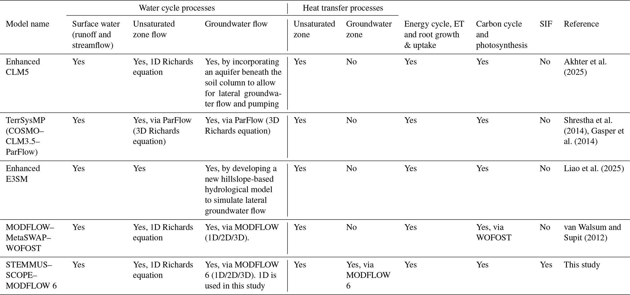
Given the limitations of both the LSMs/SPAC models and IHMs, an integrated modelling approach that combines hydrology with ecosystem functioning would result in a modelling tool that is better suited for evaluating ecosystem functioning under a changing climate. An integrated LSM-IHM or SPAC-IHM model is hereafter referred to as an integrated ecohydrological model (IEM). The advantage of an IEM is that it can simulate the full continuum of water (including groundwater), energy, and carbon fluxes at high spatio-temporal resolution within a single simulation environment. IEMs are also capable of integrating the surface and subsurface hydrology (both unsaturated and saturated zones) with plant physiological processes, as well as incorporating RS information (as inputs) for simultaneous simulation of multiple variables [i.e., soil moisture (θ), soil temperature (T_s), evapotranspiration (ET), groundwater level (GWL), groundwater temperature (GT), gross primary productivity (GPP), net ecosystem exchange (NEE), and SIF] that are vital for accurately characterizing ecosystem dynamics. Furthermore, IEMs facilitate the simulation of continuous moisture and temperature profiles from the subsurface to the top of the canopy. Table 1 lists the few existing IEMs that can physically simulate energy, carbon, and water processes, including groundwater flow. The list includes the enhanced CLM5 (Akhter et al., 2025), the Terrestrial System Modelling Platform (TerrSysMP, Shrestha et al., 2014; Gasper et al., 2014), the enhanced version (Liao et al., 2025) of the Earth system model (E3SM; Golaz et al., 2022) and the MODFLOW–MetaSWAP–WOFOST (van Walsum and Supit, 2012). While all these IEMs can simulate water processes, including detailed groundwater flow processes, they all lack the representation of groundwater heat processes and groundwater temperature simulation. Furthermore, none of them accounts for SIF simulation, which serves as a direct proxy for photosynthesis. Hence, a new IEM is needed that can physically-based integrate the groundwater processes (mass and energy) with detailed energy, carbon and SIF fluxes. The hypothesis of this study is that explicit representation of groundwater mass and energy in an IEM framework would improve quantification of the soil-plant-atmosphere continuum by: (a) improving the simulation of soil moisture and temperature profiles; (b) enabling two-way feedbacks between the unsaturated and saturated zone and their further impact on water fluxes; and (c) revealing the groundwater's influence on carbon fluxes and vegetation physiological processes such as root water uptake and photosynthesis (reflected by fluorescence). Collectively, testing these hypotheses would unravel the role of groundwater in shaping the SPAC dynamics and deepen the understanding of ecosystem functioning.

This study aims to investigate the role of groundwater in the SPAC with a focus on assessing the benefits of explicitly incorporating the groundwater component in modelling SPAC processes. In particular, the specific objectives are to investigate the impacts of the groundwater component (mass and energy) on: (1) regulating the soil profile, in terms of moisture and temperature; (2) the dynamics of the unsaturated/saturated zones and their further impact on water fluxes and root water uptake; and (3) the carbon fluxes and vegetation physiological processes (i.e. root water uptake and photosynthesis reflected by fluorescence). To address these objectives, a new IEM framework is developed by coupling the STEMMUS-SCOPE SPAC model to the MODFLOW 6 IHM and applied at three sites in the Netherlands (i.e., Loobos, Cabauw, and Veenkampen). Since STEMMUS-SCOPE is a point-based model, MODFLOW 6 is a grid-based model, and this study is the first example of coupling these two models, the ST-SC-MF6 models were set up in a vertically-stacked orientation (1-dimensional, 1D). The 1D models were assumed to be representative of the ecosystem of each of the corresponding sites. Simulated variables of interest are evaluated with and without the coupling to quantify the effect of explicitly representing groundwater within the simulations.

2 Methods

2.1 Summary of the two coupled models

STEMMUS-SCOPE (Wang et al., 2021) is a SPAC model, which is an integrated version of two separate models (STEMMUS and SCOPE). STEMMUS simulates the transfer of energy, mass, and momentum in the unsaturated zone (Zeng et al., 2011a, b; Zeng and Su, 2013). SCOPE simulates the radiative transfer in the soil, leaves, and vegetation canopies, as well as photosynthesis and non-radiative energy dissipation through convection and mechanical turbulence (van der Tol et al., 2009; Yang et al., 2021a). The coupling between STEMMUS and SCOPE enables the seamless SPAC modelling of energy, water and carbon exchanges. Additionally, STEMMUS-SCOPE allows for simulating the influence of θ and T_s variability on vegetation dynamics in terms of photosynthesis, stomatal behavior and plant water stress responses (Tang et al., 2024). More details about the STEMMUS-SCOPE coupling are described in Wang et al. (2021).

MODFLOW 6 is an IHM framework (Hughes et al., 2017) and is the latest “core” version of the well-known MODFLOW simulator of groundwater flow (GWF). In addition, MODFLOW 6 simulates other flow and transport processes, including unsaturated zone flow, overland flow, flow in surface water bodies (e.g. lakes, rivers, drains), and their interaction with the groundwater system (Langevin et al., 2017; Langevin et al., 2023). Recently, a new Groundwater Energy Transport (GWE) module, patterned after the solute transport module (Langevin et al., 2022), was added to MODFLOW 6 for simulating heat transport processes within a MODFLOW 6 simulation (Morway et al., 2025), and it is leveraged in this study.

2.2 STEMMUS-SCOPE & MODFLOW 6 coupling

The Basic Model Interface (BMI; Peckham et al., 2013; Hutton et al., 2020) was adopted as the convention for coupling STEMMUS-SCOPE to MODFLOW 6. The BMI protocol is general; it allows, via an external program or script, to control models and set their variables during runtime. By facilitating the exchange of model-calculated variables and other information between the coupled models externally, the BMI thereby eliminates the need to access (or modify) the source code(s) of the coupled models during the simulations. That protocol allows for coupling models which are written in different programming languages, as exemplified in this study (STEMMUS-SCOPE in MATLAB and MODFLOW 6 in Fortran). Hence, BMI allows for keeping up with future updates or new versions of the individual models without extensive reconfiguration.

2.2.1 BMI phases

BMI routines are commonly organized into three phases (initialize, update, finalize) as described in Fig. 2 of Hughes et al. (2022). Figure 1 shows the coupling framework of STEMMUS-SCOPE-MODFLOW 6.

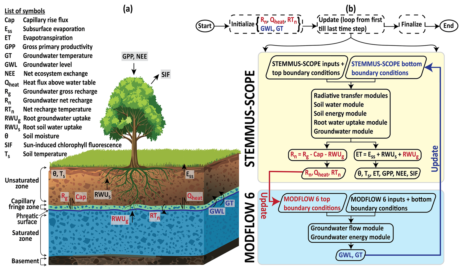
Figure 1 Schematic of the coupled STEMMUS-SCOPE and MODFLOW 6 framework: (a) illustrative diagram; (b) flowchart. The red colour indicates the processes and/or variables that are transferred from STEMMUS-SCOPE to MODFLOW 6. The blue colour indicates the processes and/or variables that are transferred from MODFLOW 6 to STEMMUS-SCOPE.

Initialize phase

The initialization phase in a BMI setup is separate from the initialization routines associated with each of the individual models (explained in Sect. 2.4.2). During the BMI initialization routine, “hooks” are established between the coupled models to facilitate the exchange of calculated values during a forward run. During the initialize phase, initialized head (i.e., GWL) and temperature (i.e., GT) of the water table are defined in STEMMUS-SCOPE. Whereas, initialized groundwater net recharge (R_n), heat flux above the water table (Q_heat), and net recharge temperature (RT_n) are defined in MODFLOW 6.

Update phase

The update phase is at the core of the coupling process (Fig. 1b). During this phase, the two models exchange variable values at the phreatic surface (the shared interface between the unsaturated zone and the saturated zone, marked by a bold blue line in the diagram of Fig. 1a). At this shared interface, STEMMUS-SCOPE requires the following bottom boundary conditions: (a) specified head (i.e. GWL) for the soil water module; and (b) specified temperature (i.e. GT) for the soil energy module; together to simulate groundwater gross recharge (R_g), capillary rise flux (Cap), root groundwater uptake (RWU_g), Q_heat, and RT_n. In turn, MODFLOW 6 requires the following upper boundary conditions: (a) specified water flux (i.e. R_n, calculated as the difference between R_g, Cap, and RWU_g) for the GWF module, and (b) specified heat flux (i.e., Q_heat) and/or specified temperature (i.e., RT_n) for the GWE module; together to simulate GWL and GT. From herein, the simulated variables (R_n, Q_heat, and RT_n) by STEMMUS-SCOPE are referred to as “STEMMUS-SCOPE variables” (marked by red colour in the flowchart of Fig. 1b), while the simulated variables by MODFLOW 6 (GWL and GT) are referred to as “MODFLOW 6 variables” (marked by blue colour in the flowchart of Fig. 1b).

The update phase runs in a looped manner (update loop), with number of updates equal to number of models' time steps. In principle, the BMI can work with different temporal discretization (number of time steps and the length of each time step) for each of the two coupled models. However, for ease of use, the same temporal discretization was used for both models in this study. For each time step: (1) MODFLOW 6 runs and updates the MODFLOW 6 variables; (2) the updated MODFLOW 6 variables are passed to STEMMUS-SCOPE (illustrated by the blue bold arrow in Fig. 1b), which are used as bottom boundary conditions by STEMMUS-SCOPE; (3) STEMMUS-SCOPE runs and updates the STEMMUS-SCOPE variables; (4) the updated STEMMUS-SCOPE variables are passed back to MODFLOW 6 (illustrated by the red bold arrow in Fig. 1b) to be used as upper boundary conditions for the next time step; and (5) updates continue until the last time step.

Finalize phase

In this phase, both models finalize their simulation, and the model outputs are exported for further analysis. The model outputs include the STEMMUS-SCOPE variables, the MODFLOW 6 variables, and other variables of interest (marked by black colour in Fig. 1) as follows: θ, T_s, root soil water uptake (RWU_s), subsurface evaporation (E_ss), ET, which is the summation of E_ss, RWU_s and RWU_g, GPP, NEE, and SIF.

MODFLOW 6 was not originally written to support BMI; however, Hughes et al. (2022) documented the restructuring of the source code to align MODFLOW 6 to support the BMI conventions. Similarly, Schilperoort (2025) and Zeng et al. (2025) documented the steps followed to make STEMMUS-SCOPE BMI-compatible. In this study, a groundwater module is also added into the source code of STEMMUS-SCOPE to: (a) recognize the effect of the saturated zone dynamics on the unsaturated zone through the MODFLOW 6 variables; and (b) prepare the necessary STEMMUS-SCOPE variables that are fed into MODFLOW 6. The groundwater module includes three main parts: (1) unsaturated zone bottom boundary; (2) recharge and capillary rise flux; and (3) root groundwater uptake.

2.2.2 Unsaturated zone bottom boundary

The bottom boundary of the unsaturated zone for the soil water module in STEMMUS-SCOPE can be defined using one of three options (Zeng and Su, 2013): (a) specified matric head (Dirichlet) boundary; (b) specified moisture flux; and (c) zero matric head (i.e. gravity drainage). In this study, option (a) is used. This bottom boundary (specified matric head) is adaptively positioned at the phreatic surface (Fig. 1a), corresponding to the GWL at each time step (Zeng et al., 2019a). The GWL value is received by STEMMUS-SCOPE from MODFLOW 6 through the BMI (Fig. 1b). Then, at the phreatic surface elevation (GWL), the specified matric head is set to zero (matric head is negative above GWL and positive below GWL). At each time step, the GWL may rise or fall, causing the phreatic surface to shift upward or downward. As a result, the thickness of the unsaturated zone decreases or increases, and the position of the bottom boundary is updated to reflect this moving boundary condition.

Similarly, for the soil energy module, a specified temperature boundary condition is used as the bottom boundary. The value of the specified temperature is the GT (Fig. 1b), received by STEMMUS-SCOPE from MODFLOW 6 through the BMI and updated at each time step.

2.2.3 Recharge and capillary rise flux

STEMMUS-SCOPE simulates two-phase mass and heat flow in the unsaturated zone using the modified Richards equation (Milly, 1982). The water flow is driven by both gravity and capillary forces (Eq. 1).

$$\begin{array}{}\text{(1)}& \begin{array}{rl}{\displaystyle \frac{\mathit{\delta }}{\mathit{\delta }t}}\left({\mathit{\rho }}_{\mathrm{L}}{\mathit{\theta }}_{\mathrm{L}}+{\mathit{\rho }}_{\mathrm{v}}{\mathit{\theta }}_{\mathrm{v}}\right)& ={\displaystyle \frac{-\mathit{\delta }}{\mathit{\delta }z}}\left(q_{\mathrm{Lh}}+q_{\mathrm{LT}}+q_{\mathrm{vh}}+q_{\mathrm{vT}}\right)-S\\ & ={\mathit{\rho }}_{\mathrm{L}}{\displaystyle \frac{\mathit{\delta }}{\mathit{\delta }z}}\left[K\left({\displaystyle \frac{\mathit{\delta }\mathit{\psi }}{\mathit{\delta }z}}+\mathrm{1}\right)+D_{\mathrm{Ta}}{\displaystyle \frac{\mathit{\delta }T}{\mathit{\delta }z}}\right]\\ & +{\displaystyle \frac{\mathit{\delta }}{\mathit{\delta }z}}\left[D_{\mathrm{vh}}{\displaystyle \frac{\mathit{\delta }\mathit{\psi }}{\mathit{\delta }z}}+D_{\mathrm{vT}}{\displaystyle \frac{\mathit{\delta }T}{\mathit{\delta }z}}\right]-S\end{array}\end{array}$$

where ρ_L and ρ_v (kg m⁻³) are the density of liquid water and water vapour, respectively; θ_L and θ_v (m³ m⁻³) are the soil liquid and vapour volumetric water content, respectively; q_Lh and q_LT (kg m⁻² s⁻¹) are the soil liquid water fluxes driven by the soil matric potential gradient $\left(\frac{\mathit{\delta }\mathit{\psi }}{\mathit{\delta }z}\right)$ and temperature gradient $\left(\frac{\mathit{\delta }T}{\mathit{\delta }z}\right)$, respectively; q_vh and q_vT (kg m⁻² s⁻¹) are the soil water vapour fluxes driven by the $\frac{\mathit{\delta }\mathit{\psi }}{\mathit{\delta }z}$ gradient and the $\frac{\mathit{\delta }T}{\mathit{\delta }z}$ gradient, respectively; K is the unsaturated hydraulic conductivity (m s⁻¹); D_Ta (m² s⁻¹ K⁻¹) is the transport coefficient of the adsorbed liquid flow due to temperature gradient; D_vh (kg m⁻² s⁻¹) is the isothermal vapour conductivity; D_vT (kg m⁻¹ s⁻¹ K⁻¹) is the thermal vapour diffusion coefficient, and S is the sink term (m s⁻¹). More details of the equation are in Zeng et al. (2011a, b) and Zeng and Su (2013).

As explained in Sect. 2.2.1 and 2.2.2, the GWL is adopted as the bottom boundary condition of the unsaturated zone in STEMMUS-SCOPE. Consequently, a capillary fringe zone is formed above the phreatic surface (Fig. 1a), where water is pulled up from the saturated zone by capillary forces. Moreover, when precipitation infiltrates into the unsaturated zone and percolates downward, it has to go through the capillary fringe zone and continue downward as R_g to the saturated zone. Hence, the capillary fringe zone includes both the R_g and the Cap. Both R_g and Cap, the latter contributes to groundwater evaporation (Balugani et al., 2017), are calculated from the summation of q_Lh, q_LT, q_vh, and q_vT fluxes (Eq. 2) at the capillary fringe zone. The result of that summation determines whether the calculated flux (Q, Eq. 2a) represents R_g or Cap. If the summation is negative (Eq. 2b), it means the flow direction is downward, and the R_g term is dominant. In contrast, if the summation is positive (Eq. 2c), it means the flow direction is upward, and the Cap term is dominant. In STEMMUS-SCOPE, upward fluxes (capillary rise) are positive, while downward fluxes (gravity drainage) are negative. However, MODFLOW 6 uses the opposite sign convention. Therefore, the $R_{\mathrm{g}}/\mathrm{Cap}$ sign needs to be inverted, when transferred to MODFLOW 6 through BMI.

$$\begin{array}{}\text{(2a)}& {\displaystyle }Q=q_{\mathrm{Lh}}+q_{\mathrm{LT}}+q_{\mathrm{vh}}+q_{\mathrm{vT}}\text{(2b)}& {\displaystyle }{R}_{\mathrm{g}}=\left\{\begin{array}{ll}-Q& \mathrm{if}Q<\mathrm{0}\\ \mathrm{0}& \mathrm{if}Q\ge \mathrm{0}\end{array}\right.\text{(2c)}& {\displaystyle }\mathrm{Cap}=\left\{\begin{array}{ll}Q& \mathrm{if}Q\ge \mathrm{0}\\ \mathrm{0}& \mathrm{if}Q<\mathrm{0}\end{array}\right.\end{array}$$

2.2.4 Root groundwater uptake

The root water uptake (RWU) is calculated in STEMMUS-SCOPE based on a resistance scheme that takes into account the hydraulic gradient between the soil water potential (ψ_s) and the leaf water potential (ψ_l) (Eq. 3). The root water uptake module, developed by Wang et al. (2021), takes into account the θ as the only source of water for the roots (root soil water uptake, RWU_s), meaning that RWU=RWU_s. The RWU_s is calculated for all the soil layers that are above the maximum rooting depth (d_max).

$${\mathrm{RWU}}_{\mathrm{s}}=\sum _{i=\mathrm{1}}^n{\displaystyle \frac{{\mathit{\psi }}_{\mathrm{s},\mathrm{i}}-{\mathit{\psi }}_{\mathrm{l}}}{r_{\mathrm{s},i}+r_{\mathrm{r},i}+r_{\mathrm{x},i}}}$$

and

$$\begin{array}{}\text{(3)}& \mathrm{RWU}={\mathrm{RWU}}_{\mathrm{s}}\end{array}$$

where ψ_s,i is the soil water potential of layer i (m), ψ_l is leaf water potential (m), r_s,i is the soil hydraulic resistance (s m⁻¹), r_r,i is the root resistance to water flow radially across the roots (s m⁻¹), and r_x,i is the plant's axial resistance to flow from the root xylem to the leaves (s m⁻¹).

However, the roots can uptake water from an additional source (root groundwater uptake, RWU_g) if the roots have access to groundwater (GWL is above d_max). As explained in Sect. 2.2.1 and 2.2.2, the GWL is adopted as the bottom boundary condition of the unsaturated zone for the soil water module in STEMMUS-SCOPE; hence, the RWU can also be influenced. The RWU calculations were updated by splitting it into two components (RWU_s and RWU_g, Eq. 4). The RWU_s is for the soil layers that are above the capillary fringe and above d_max (Eq. 5), and the RWU_g is for the soil layers that are below the capillary fringe zone and above d_max (Eq. 6). The RWU_s and RWU_g are calculated by replacing the ψ_s,i in Eq. (3) with the updated ψ_s,i (due to the effect of GWL) in Eq. (5), and with the groundwater potential (ψ_g,i) in Eq. (6), respectively. For soil layers below d_max, RWU = 0.

$$\begin{array}{}\text{(4)}& {\displaystyle }\mathrm{RWU}={\mathrm{RWU}}_{\mathrm{s}}+{\mathrm{RWU}}_{\mathrm{g}}\text{(5)}& {\displaystyle }{\mathrm{RWU}}_{\mathrm{s}}=\sum _{i=\mathrm{1}}^n{\displaystyle \frac{{\mathit{\psi }}_{\mathrm{s},\mathrm{i}}-{\mathit{\psi }}_{\mathrm{l}}}{r_{\mathrm{s},i}+r_{\mathrm{r},i}+r_{\mathrm{x},i}}}\end{array}$$

for the soil layers above capillary fringe zone and above d_max.

$$\begin{array}{}\text{(6)}& {\mathrm{RWU}}_{\mathrm{g}}=\sum _{i=\mathrm{1}}^n{\displaystyle \frac{{\mathit{\psi }}_{\mathrm{g},i}-{\mathit{\psi }}_{\mathrm{l}}}{r_{\mathrm{s},i}+r_{\mathrm{r},i}+r_{\mathrm{x},i}}}\end{array}$$

for the soil layers below capillary fringe zone and above d_max.

2.3 Study sites and data

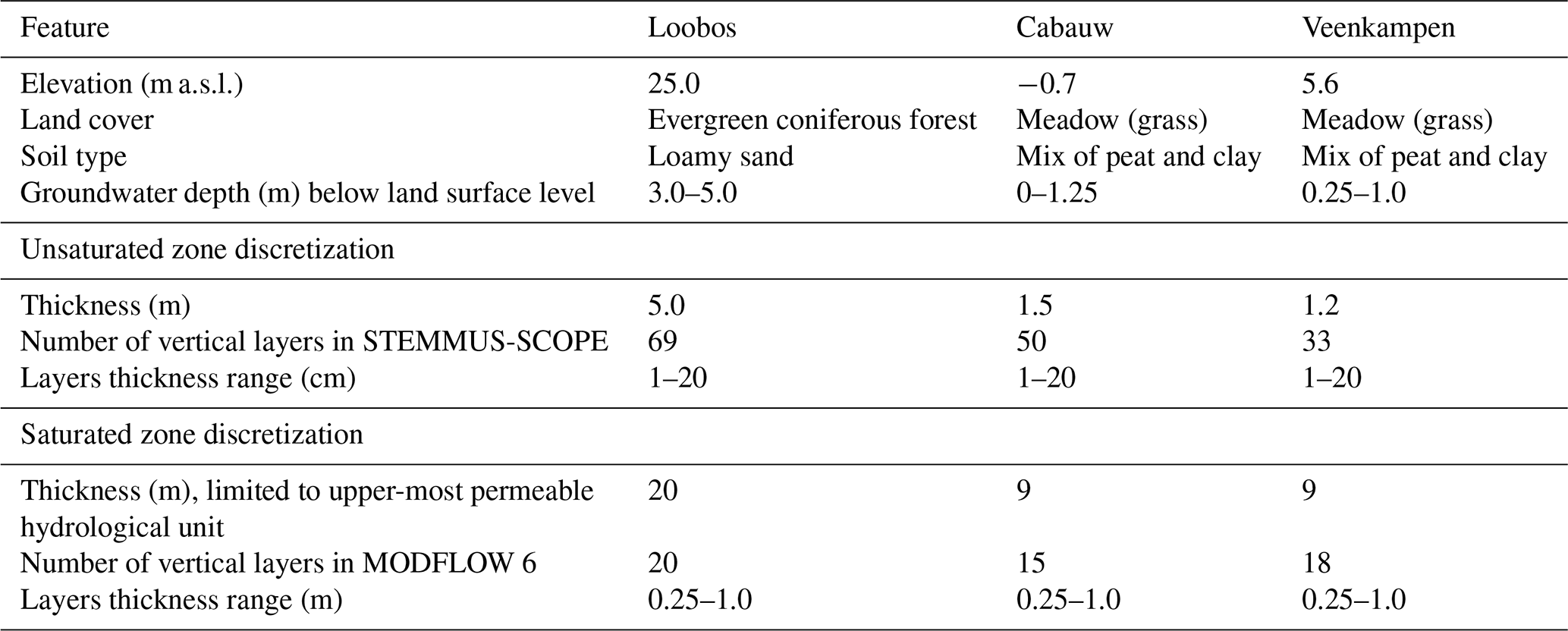
The proposed model coupling was applied to three sites in the Netherlands covering both forest (Loobos) and meadow (Cabauw and Veenkampen) ecosystems (Fig. 2). Those three sites were selected because: (a) they provide comprehensive in-situ measurements spanning the water, energy, and carbon cycles, including meteorological forcing, different observations such as θ and T_s profiles, eddy covariance flux measurements (e.g. ET, GPP, and NEE), groundwater variables (i.e. GWL and GT), and vegetation characteristics (e.g. SIF) – such data density is essential for rigorously testing the hypothesis of this study and evaluating the developed coupled modelling framework; and (b) the sites represent two dominant Dutch landscapes (forest on sandy soil; meadow on clay/peat), allowing preliminary assessment of model transferability across ecosystem types. The three sites feature the typical temperate climate of the Netherlands, with an annual average precipitation of 700–900 mm yr⁻¹ (Buishand et al., 2010; Brakkee et al., 2022), and an annual average air temperature of 10.5 °C (Bense and Kurylyk, 2017; Jansen et al., 2023). The Loobos site is located in the forested area of the Veluwe in the central part of the Netherlands, with an elevation of 25.0 m above sea level (a.s.l.; Table 2). The land cover is evergreen coniferous forest, and the soil type is loamy sandy soil (Heinen et al., 2021). The groundwater depth ranges from 3.0 to 5.0 m below land surface (b.l.s.; van der Molen et al., 2024; Zhao et al., 2026). The Cabauw site is located in the central western region of the Netherlands, with an elevation of −0.7 m a.s.l. (Table 2). The land cover is grass, and the soil is a mixture of clay and peat (Heinen et al., 2021). The groundwater depth ranges from 0 to 1.25 m b.l.s. The Veenkampen site is located in the Veluwe area in the central part of the Netherlands, with an elevation of 5.6 m a.s.l. (Table 2). The land cover is grass, and the soil is thin peat underlain by a clayey sand (Heinen et al., 2021). The groundwater depth ranges from 0.25 to 1.0 m b.l.s.

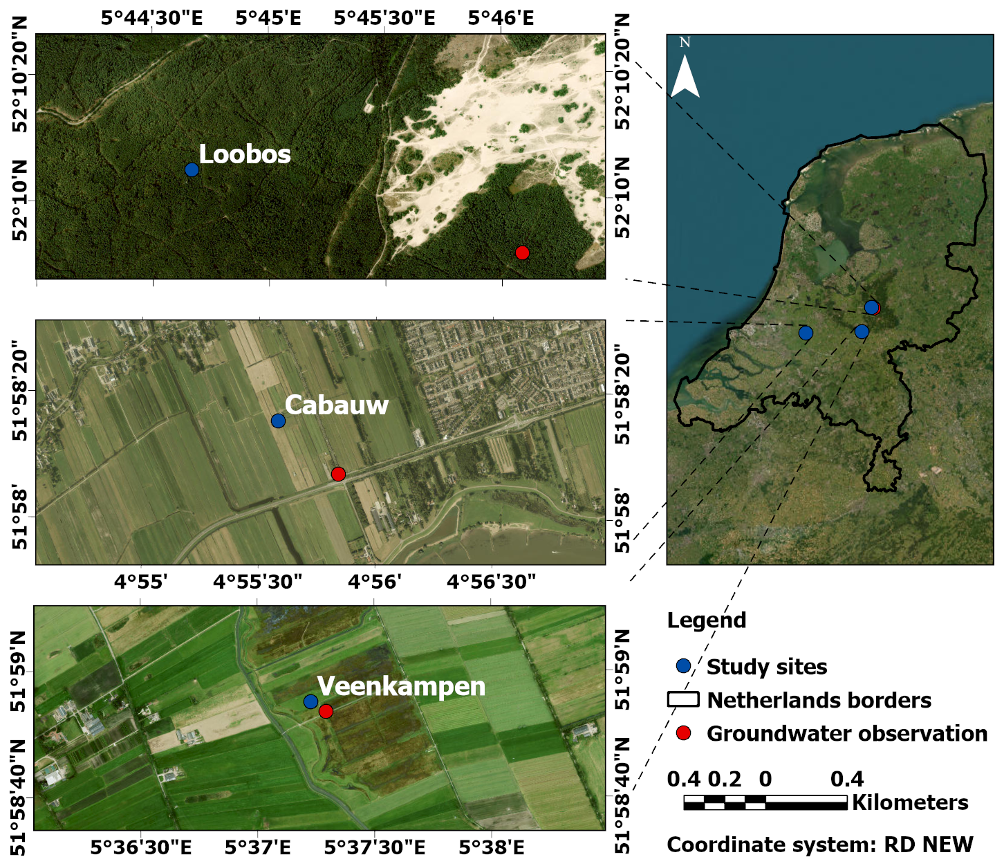
Figure 2 Location of the three study sites. Images are generated from the day 20 March 2025, using the ArcGIS Pro Basemap © ESRI software (Powered by Esri).

Table 2 Summary of site characteristics and model discretization.

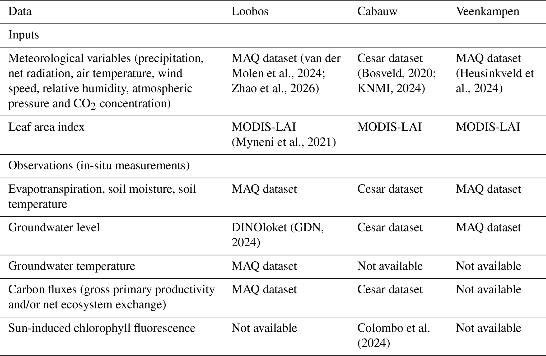
The forcing inputs and observations data for the three sites were collected from different sources (Table 3). The Meteorology and Air Quality (MAQ) dataset is an open-access collection of harmonized meteorological variables, eddy covariance fluxes, and soil observations for the Loobos and Veenkampen sites, maintained by Wageningen University (van der Molen et al., 2024; Heusinkveld et al., 2024; Zhao et al., 2026). Similarly, the Cesar dataset, operated by the Royal Netherlands Meteorological Institute (KNMI), provides a wide suite of measurements including RS, eddy covariance, surface, soil and hydrological measurements at the Cabauw site (Bosveld, 2020; KNMI, 2024). The forcing inputs include time series of the meteorological inputs (i.e., precipitation, net radiation, air temperature, wind speed, relative humidity, atmospheric pressure, and CO₂ concentration) and the leaf area index (LAI). For Loobos and Veenkampen, the meteorological inputs and observation datasets were retrieved from the MAQ dataset, while those for the Cabauw site were retrieved from the Cesar dataset (Table 3). The LAI for the three sites was retrieved from the RS MODIS product (MCD15A3H v061, Myneni et al., 2021). The observation datasets include time series of θ, T_s, ET, GPP, NEE, GWL, GT, and SIF. Among all observations, θ and T_s profiles, as well as ET, were available for most of the simulation period, except for short gaps, at the three sites. The ET observations were derived from eddy covariance towers at the three sites, representing actual ET. GPP was available only at the Loobos site for the period 2016–2021, while NEE was available only at the Cabauw site for the period 2016–2020. GWL was available at Cabauw and Veenkampen from observation wells located close to the main measurement infrastructure (i.e. eddy covariance tower) (Fig. 2). Whereas, at Loobos, GWL was not available exactly within the site, but obtained from the nearest available observation point (approximately 500 m away; Fig. 2) via the Data and Information of the Dutch Subsurface (DINOloket) dataset (GDN, 2024). GT was available only at the Loobos site for one year (1 April 2023–31 March 2024). SIF observations were available only at Cabauw on certain days in 2022 and 2023 and were collected by Colombo et al. (2024). All the collected datasets were processed and formatted to be compatible with the needed formats (NetCDF for STEMMUS-SCOPE and ASCII for MODFLOW 6).

Table 3 Datasets acquisition at the three sites.

2.4 Models' setup

For brevity, from herein, when comparing simulations, the standalone STEMMUS-SCOPE simulation is referred to as “ST-SC” and the coupled STEMMUS-SCOPE-MODFLOW 6 simulation is referred to as “ST-SC-MF6”. The term “STEMMUS-SCOPE” is reserved for referencing the underlying model structure or parameter settings that are shared by both standalone and coupled simulations.

2.4.1 Temporal and spatial discretization

Both ST-SC and ST-SC-MF6 models of the three sites used a three-month model initialization phase (i.e. “spin-up”) that extended from 1 January to 31 March 2016. After this, the simulation was run for a period of 8 years (1 April 2016–31 March 2024). The total simulation had 144 624 half-hourly time steps.

The unsaturated zone in STEMMUS-SCOPE was modelled with site-specific total thicknesses – each equals or exceeds the site's maximum observed water table depth (Table 2). The unsaturated zone was vertically discretized into 69, 50, and 33 layers for Loobos, Cabauw, and Veenkampen, respectively (Table 2). The thickness of the layers was variable (minimum of 1 cm and maximum of 20 cm), started with fine resolution near the surface (1 cm), gradually increased to 20 cm, then gradually decreased again to 5 cm near the water table fluctuation zone.

The MODFLOW 6 models were horizontally discretized into a single cell that is 1 m by 1 m, and were vertically discretized into 20, 15, and 18 layers for the Loobos, Cabauw and Veenkampen sites, respectively (Table 2). The layering information was retrieved from the BRO GeoTOP v1.6.1 geological model (TNO – GDN, 2025a) and the BRO REGIS II v2.2.3 hydrogeological model (TNO – GDN, 2025b). Since the models were 1D models in the vertical direction, lateral flow considerations were neglected. To minimize the effect of this neglect, the saturated zone simulation was limited to the upper-most permeable hydrogeological unit, which terminates at a depth of 20 m b.l.s. for Loobos and 9 m for both the Cabauw and Veenkampen sites. This permeable hydrogeological unit was then sub-divided into thinner layers, started with a thickness of 0.25 m, then smoothly increased to 0.5, 0.75, and 1 m. At the base of the bottom-most active layer, a specified flux boundary condition was applied to compensate for the vertical flow of the excluded deeper hydrogeological units.

2.4.2 Initial and boundary conditions

Each model of the three sites was initialized by an initial θ and T_s for STEMMUS-SCOPE, and an initial GWL and GT for MODFLOW 6. The initial θ, T_s, GWL, and GT values were retrieved from the collected datasets (Table 3) of the three sites as follows: (a) 0.1, 5 °C, 21.5 m, and 10 °C for Loobos, (b) 0.6, 5 °C, −0.8 m and 10.5 °C for Cabauw, and (c) 0.75, 5 °C, 5.1 m, and 11 °C for Veenkampen.

The top boundary of the soil water module in STEMMUS-SCOPE was a specified flux (precipitation, input retrieved from the collected datasets in Table 3), and the bottom boundary was the GWL (received from MODFLOW 6). The top boundary of the soil energy module in STEMMUS-SCOPE was a specified temperature (air temperature, input retrieved from the collected datasets in Table 3), and the bottom boundary was the GT (received from MODFLOW 6). The top boundary of the GWF module of the saturated zone in MODFLOW 6 was the R_n (received from STEMMUS-SCOPE), and the bottom boundary was a specified flux (unknown value that was initially set to 0.0005 m d⁻¹ and calibrated later). The top boundary of the GWE module of the saturated zone in MODFLOW 6 was the Q_heat and RT_n (received from STEMMUS-SCOPE), and the bottom boundary was a specified heat flux (unknown value that was initially set to 0.05 W m⁻² and calibrated later).

2.4.3 Model parameters and calibration/validation

Both STEMMUS-SCOPE and MODFLOW 6 models have several parameters – herein, only the parameters that had a high impact on the simulations (based on an earlier sensitivity analysis) are calibrated and listed in Table 4. The main parameters that govern the flow simulation in STEMMUS-SCOPE were: the vertical saturated hydraulic conductivity of the unsaturated zone (K_sat), residual water content (θ_r), saturated water content (θ_s), empirical coefficients of the Van Genuchten equation (α and n), and d_max. In MODFLOW 6, the main aquifer parameters were: the horizontal (K_h) and vertical (K_v) hydraulic conductivity, specific storage (S_s), and specific yield (S_y). Both STEMMUS-SCOPE and MODFLOW 6 used the same thermal parameters to simulate the heat transfer in both the unsaturated and the saturated zones, including: thermal conductivity of solids (K_T), specific heat capacity of solids (c_s), and bulk density (ρ_s). As explained in Sect. 2.4.1, the soil profiles at each site were discretized into multiple vertical layers (Table 2) to account for soil heterogeneity. Initially, all layers were assigned uniform values for each parameter. During the calibration procedure, these parameters were updated individually for each layer to reflect the vertical variability of the θ and T_s measurements. The ranges of the calibrated values for each parameter across the layers are summarized in Table 4.

Table 4 Models' tuned parameters.

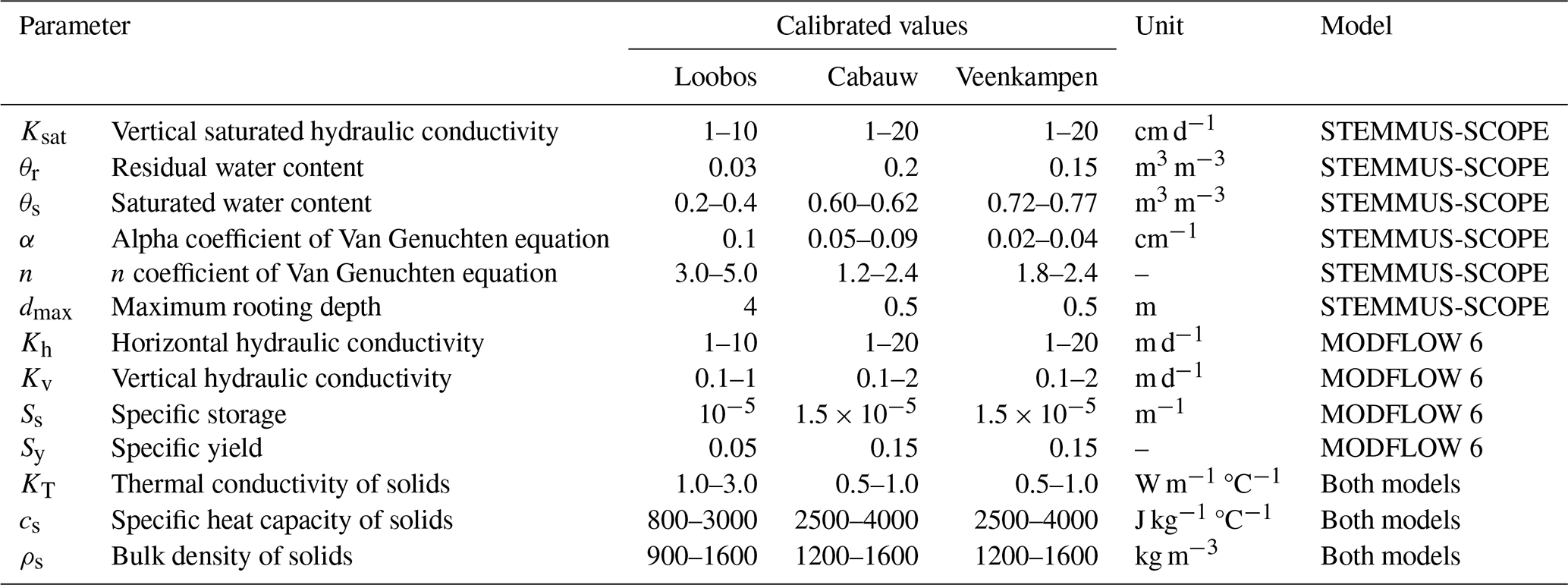
The 8-year simulation period was divided into a 4-year calibration period (1 April 2016–31 March 2020), followed by a 4-year validation period (1 April 2020–31 March 2024). The collected observation datasets (Table 3) were used as calibration/validation state variables for the calibration/validation periods, respectively. The models were calibrated by trial and error until satisfactory qualitative (graphical) and quantitative (statistical) matches between the simulated variables and their observed equivalents were achieved. To ensure an unbiased comparison, both ST-SC and ST-SC-MF6 setups across the three sites were initialized using identical baseline parameter values derived from each site's measurements and literature. The manual calibration for both setups followed the same iterative step-by-step procedure within identical, physically realistic parameter bounds (Table 4). The goodness of fit was assessed using two statistical metrics: the Kling–Gupta efficiency (KGE; Gupta et al., 2009) and the root mean square error (RMSE). The KGE value can range from negative infinity to 1 and was deemed acceptable, when it was larger than zero (Knoben et al., 2019). The RMSE value was deemed acceptable, when it was minimized to 0.1 m³ m⁻³, 2 °C, 0.5 m, 1 °C, 1 mm d⁻¹, 3 g C m⁻² d⁻¹, 5 g C m⁻² d⁻¹, and 0.25 mW m⁻² µm⁻¹ sr⁻¹ for θ, T_s, GWL, GT, ET, GPP, NEE, and SIF, respectively, as similar ranges were indicated in former studies (Lekula and Lubczynski, 2019; Pacheco-Labrador et al., 2019; Thum et al., 2019; van der Velde et al., 2023; Benz et al., 2024; Qian et al., 2024; Yang and Lei, 2024; Wang et al., 2026). Additionally, to evaluate whether the increased complexity of ST-SC-MF6 is justified relative to parameter addition, the Akaike Information Criterion (AIC; Akaike, 1973) was computed across all observed variables.

3 Results

3.1 Overall models' performance

At each of the three study sites, the coupled ST-SC-MF6 framework consistently outperformed the standalone ST-SC model across most of the simulated variables (Tables 5, 6 and Figs. 4–9). This superior performance stems from better physical representation of dynamic surface–subsurface hydro-thermal interactions in the coupled ST-SC-MF6 (as discussed in detail in subsequent sections) – which are structurally missing in the standalone ST-SC model – rather than discrepancies in parameter search effort. Furthermore, the AIC evaluation (details omitted here for brevity) yielded substantially lower values for ST-SC-MF6 across almost all observations as compared to the ST-SC, confirming that the enhanced predictive performance strongly justifies the added model parameterization, with the sole exception of GPP at Loobos where groundwater dynamics exert minimal control.

Table 5 KGE values of the calibration state variables for the STEMMUS-SCOPE (ST-SC) and STEMMUS-SCOPE-MODFLOW 6 (ST-SC-MF6) models at the three sites over the entire simulation period.

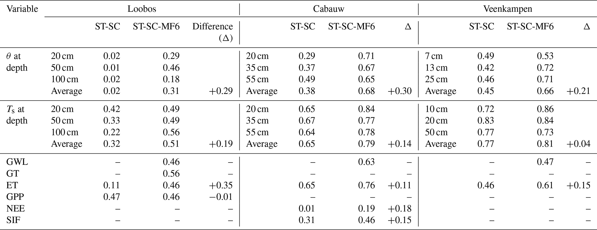
Table 6 RMSE values of the calibration state variables for the STEMMUS-SCOPE (ST-SC) and STEMMUS-SCOPE-MODFLOW 6 (ST-SC-MF6) models at the three sites over the entire simulation period.

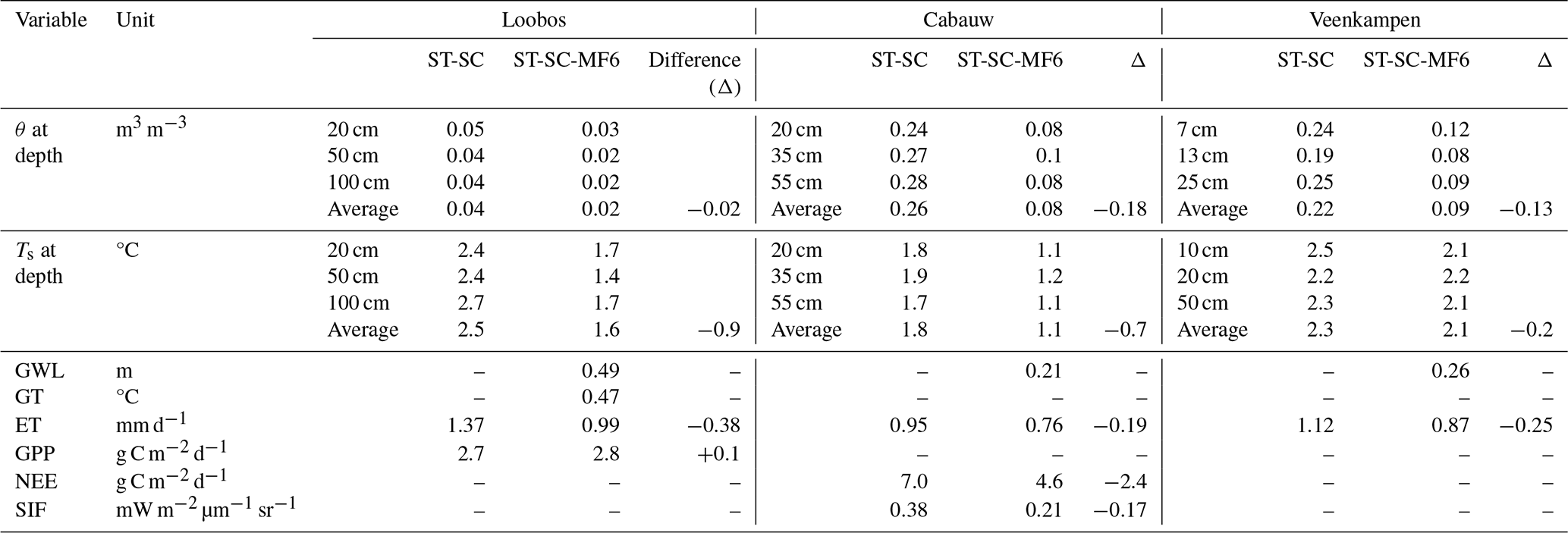
The θ simulation of the ST-SC-MF6 demonstrated better agreement with the observations during both the calibration and validation periods as compared to the ST-SC simulations at the three sites. The depth-averaged KGE values of θ were increased by 0.29 at Loobos, 0.30 at Cabauw, and 0.21 at Veenkampen (Table 5), while the depth-averaged RMSE values were decreased by 0.02, 0.18, and 0.13 at Loobos, Cabauw and Veenkampen, respectively (Table 6).

The T_s improvement of the ST-SC-MF6 simulations was site-dependent. The depth-averaged KGE values of T_s were increased by 0.19 and 0.14 at Loobos and Cabauw, respectively, while increasing slightly in Veenkampen by 0.04 (Table 5). Corresponding RMSE reductions were 0.9, 0.7, and 0.2 °C at Loobos, Cabauw and Veenkampen, respectively (Table 6).

The ET improvement of the ST-SC-MF6 simulations was consistent across the three sites, with KGE increases of 0.35, 0.11, 0.15, accompanied by RMSE reductions of 0.38, 0.19, 0.25 mm d⁻¹ at Loobos, Cabauw and Veenkampen (Tables 5 and 6), respectively.

The carbon flux responses were site-dependent. At Cabauw, the KGE of NEE increased by 0.18, and the RMSE decreased by 2.4 g C m⁻² d⁻¹ (Tables 5 and 6). Whereas, at Loobos, the GPP showed negligible changes between the ST-SC and ST-SC-MF6 simulations, i.e. changes in KGE and RMSE values were limited to 0.01 and 0.1 g C m⁻² d⁻¹, respectively (Tables 5 and 6).

For SIF at Cabauw, improvement of the ST-SC-MF6 simulation was satisfactory, with a KGE increase of 0.15 and RMSE reduction of 0.17 mW m⁻² µm⁻¹ sr⁻¹, respectively (Tables 5 and 6).

Considering the groundwater variables (GWL and GT) in the ST-SC-MF6 simulation, the KGE values for GWL were 0.46 at Loobos, 0.63 at Cabauw, and 0.47 at Veenkampen, and RMSE values of 0.49, 0.21, and 0.26 m, respectively. For GT at Loobos, the KGE value was 0.56 with a corresponding RMSE of 0.47 °C.

3.2 Saturated zone dynamics

The coupled ST-SC-MF6 model reproduced GWL and GT dynamics with overall satisfactory KGE and RMSE performance across the three sites (Sect. 3.1). At the three sites, the ST-SC-MF6 models successfully captured the observed GWL rise during wet periods and drawdown during dry periods (Fig. 3). At Cabauw and Veenkampen, the shallow water table exhibited pronounced groundwater – soil coupling, which directly influenced root-zone moisture and propagated upward to ecosystem fluxes. In contrast, at Loobos, the relatively moderate groundwater depths and poor soil characteristics resulted in weak hydraulic connectivity with the unsaturated zone, limiting its influence on upper soil layers' moisture dynamics. However, the ST-SC-MF6 model successfully reproduced the seasonal GT variability (Fig. 3) with satisfactory KGE and RMSE performances, demonstrating the ability of the coupled model in simulating the subsurface heat transfer and its influence on the unsaturated zone thermal dynamics (Sect. 3.3.2). Although observed GT data in Loobos were available for only one year (1 April 2023–31 March 2024) during the validation period, the seasonal GT fluctuations from that period were assumed to be representative of the site's thermal regime and exceptionally were used to calibrate the thermal parameters (K_T and c_s; Table 4) within the calibration period (1 April 2016–31 March 2020). Overall, producing simulated groundwater variables, i.e. GWL and GT, with satisfactory performance enabled a mechanistic assessment of groundwater contributions, in terms of mass and heat, to different soil and vegetation processes at the three sites as explained in the following subsections (Sect. 4.1–4.4).

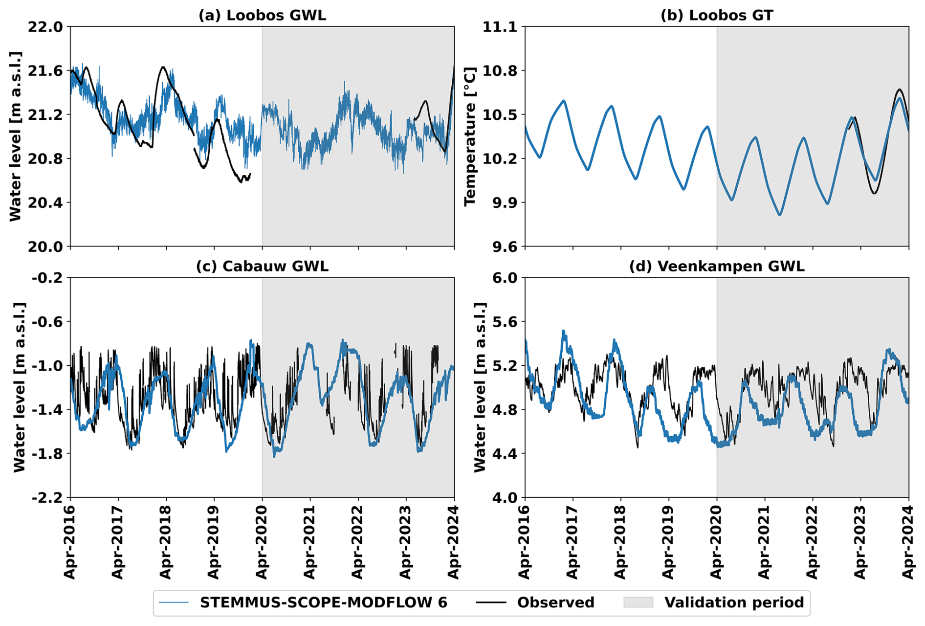
Figure 3 Comparison of half-hourly simulated groundwater level (GWL) and groundwater temperature (GT) values by STEMMUS-SCOPE-MODFLOW 6 (blue lines) and observed ones (black lines) during the calibration period (1 April 2016–31 March 2020) and the validation period (1 April 2020–31 March 2024; grey shaded) at: Loobos (a, b), Cabauw (c), and Veenkampen (d). Land surface elevation values of the three sites are shown in Table 2.

Although lateral groundwater flow was not simulated in the present 1D applications, calibrating (i.e., adjusting the aquifer parameters) the ST-SC-MF6 models against the observed GWL allowed the models to capture the local water table state. Nevertheless, incorporating lateral groundwater flow in future 2D/3D applications would likely improve model process realism and predictive capability, particularly when assessing groundwater as a managed water resource and its broader role in ecosystem functioning.

3.3 Unsaturated zone dynamics

3.3.1 Soil moisture

Figure 4 presents half-hourly observations and simulated outputs from the ST-SC and the ST-SC-MF6 models for θ at available depths at the three sites. The improvements in capturing the θ dynamics within ST-SC-MF6 simulations were evident at all soil depths, but were most pronounced during the wet periods at Cabauw and Veenkampen sites, characterized by shallow groundwater depths (0–1.25 m). At these two sites, the ST-SC-MF6 models successfully captured the θ peaks that occurred during winter periods, along different soil depths (0.6 m³ m⁻³ at Cabauw and 0.75 m³ m⁻³ at Veenkampen), representing near-saturation conditions. Those peaks reflect strong connectivity between soil and groundwater and the strong influence of groundwater on the soil profiles. In contrast, the ST-SC models underestimated these winter θ peaks, as the absence of groundwater limited the θ profile's ability to reach saturation conditions. At Loobos, groundwater depth was relatively moderate (3.0–5.0 m), and had limited influence on the θ dynamics. Thus, the improvement of the θ simulation of the ST-SC-MF6 over the ST-SC model at Loobos was less associated with direct groundwater feedback and more related to improved model structure and parameter calibration within the ST-SC-MF6 model.

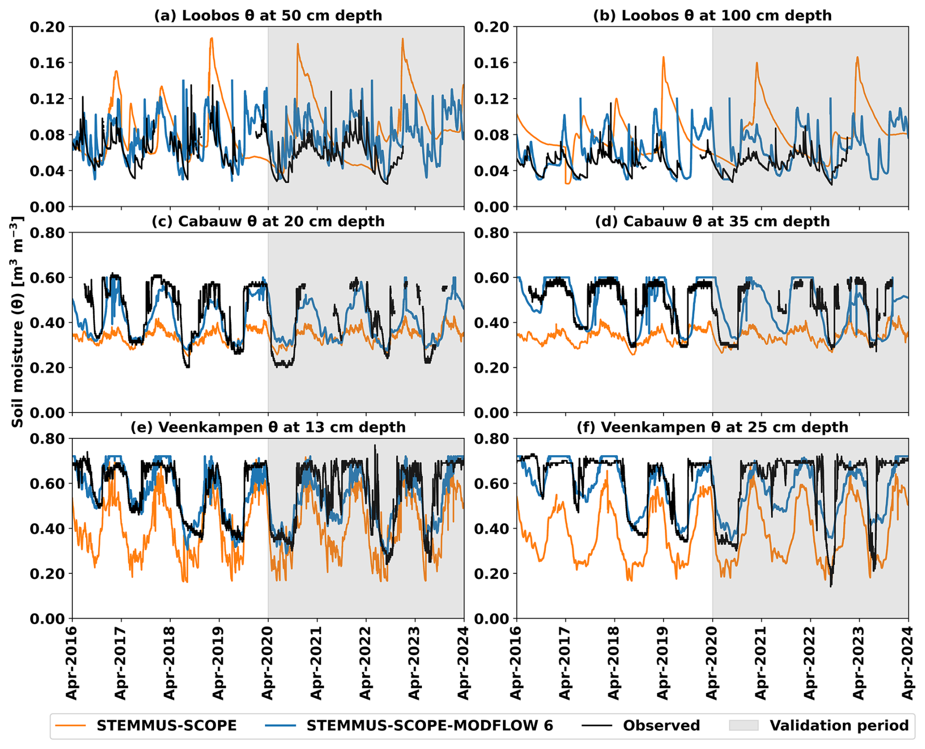
Figure 4 Comparison of half-hourly simulated soil moisture (θ) values by STEMMUS-SCOPE (orange lines), by STEMMUS-SCOPE-MODFLOW 6 (blue lines), and observed ones (black lines) during the calibration period (1 April 2016–31 March 2020) and the validation period (1 April 2020–31 March 2024; grey shaded) for: Loobos at depth: (a) 50 cm, (b) 100 cm; Cabauw at depth: (c) 20 cm, (d) 35 cm; and Veenkampen at depth: (e) 13 cm, (f) 25 cm.

3.3.2 Soil temperature

Figure 5 presents half-hourly observations and simulated outputs from the ST-SC and the ST-SC-MF6 models for T_s at available depths at the three sites. The ST-SC-MF6 model showed a closer agreement with the observations than the ST-SC model at the three sites, but this was more pronounced at Loobos. The GT observations were only available at Loobos, enabling a direct assessment of groundwater influence on T_s, unlike the case at Cabauw and Veenkampen. At Loobos, the ST-SC-MF6 simulation well captured the T_s dynamics (Fig. 5a and b). In contrast, the ST-SC simulation showed an overestimation of the θ amplitude (fluctuations), which reduced (dampened) the T_s amplitude, leading to lower T_s peaks and higher T_s troughs than the observations. Similarly, at Cabauw, the ST-SC-MF6 simulation captured well the T_s dynamics, while in contrast, the ST-SC simulation showed an overestimation of the T_s amplitude, leading to higher T_s peaks and lower T_s troughs than the observations (Fig. 5c and d). At Veenkampen, both models generally reproduced the seasonal T_s patterns and corresponded well with the observations, but exhibited a systematic tendency to slightly overestimate T_s amplitudes along the entire soil profiles (Fig. 5e and f).

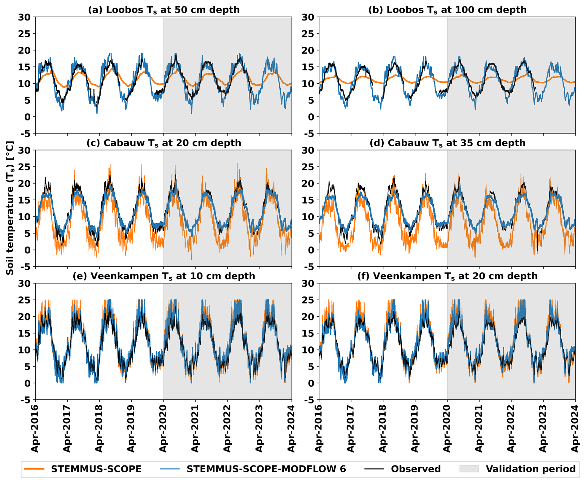
Figure 5 Comparison of half-hourly simulated soil temperature (T_s) values by STEMMUS-SCOPE (orange lines), by STEMMUS-SCOPE-MODFLOW 6 (blue lines), and observed ones (black lines) during the calibration period (1 April 2016–31 March 2020) and the validation period (1 April 2020–31 March 2024; grey shaded) for: Loobos at depth: (a) 50 cm, (b) 100 cm; Cabauw at depth: (c) 20 cm, (d) 35 cm; and Veenkampen at depth: (e) 10 cm, (f) 20 cm.

3.4 Evapotranspiration

Figure 6 illustrates daily observed and simulated ET from the ST-SC and ST-SC-MF6 models at the three sites. The zoom windows in Fig. 6 highlight the results during a dry period example in the calibration period (1 June–30 September 2019) and in the validation period (1 June–30 September 2021). Overall, at the three sites, the ST-SC-MF6 models exhibited a better match with the ET observations, particularly during the dry periods, as compared to the ST-SC models. The ST-SC simulations showed rapid ET declines during the highlighted dry period examples, when precipitation declined, leading to θ limitation. In contrast, the ST-SC-MF6 simulations maintained higher ET rates during those dry period examples due to the sustained water supply from groundwater. This buffering effect reduced underestimation of the simulated ET and better captured the observations.

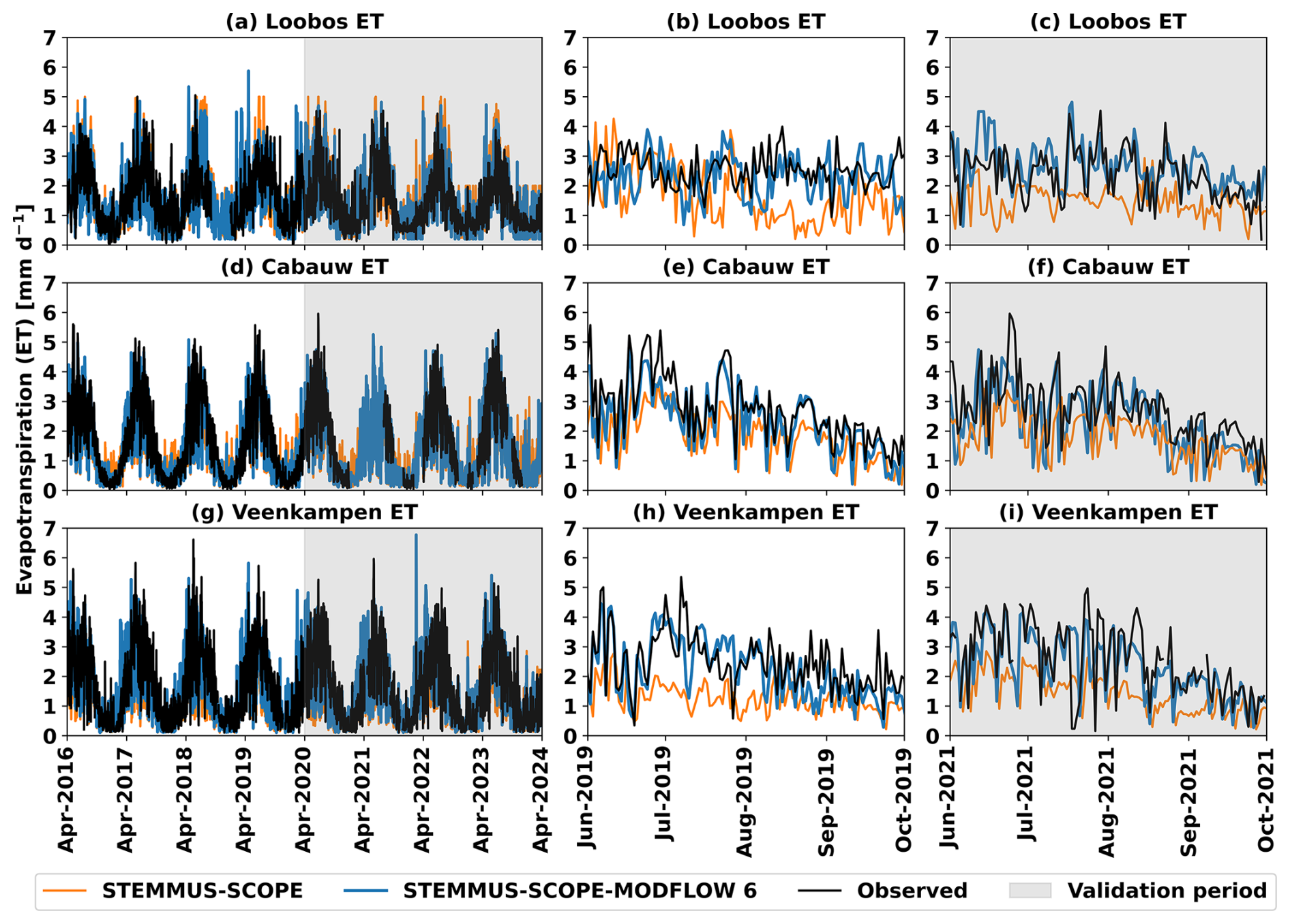
Figure 6 Comparison of daily simulated evapotranspiration (ET) values by STEMMUS-SCOPE (orange lines), by STEMMUS-SCOPE-MODFLOW 6 (blue lines), and observed ones (black lines) during the calibration period (1 April 2016–31 March 2020) and the validation period (1 April 2020–31 March 2024; grey shaded) at: (a) Loobos, (d) Cabauw, (g) Veenkampen; with windows zooming (b, e, h) in a dry period example in the calibration period (1 June–30 September 2019), and (c, f, i) in a dry period example in the validation period (1 June–30 September 2021).

3.5 Carbon fluxes and SIF

Figure 7 illustrates daily observations and simulated carbon fluxes (GPP at Loobos and NEE at Cabauw) from the ST-SC and ST-SC-MF6 models, with zoom windows to highlight the results during a dry period example in the calibration period (1 June–30 September 2019) and in the validation period (1 June–30 September 2020). At Loobos, groundwater influence on θ dynamics was weak, so GPP simulations were largely unchanged, and both ST-SC and ST-SC-MF6 models showed satisfactory agreement with the observations during the simulation period, including the dry periods (Fig. 7b and c). While at Cabauw, where strong groundwater influence on θ dynamics was observed, the ST-SC-MF6 model demonstrated a better match with the NEE observations, particularly during the dry periods (Fig. 7e and f), as compared to ST-SC.

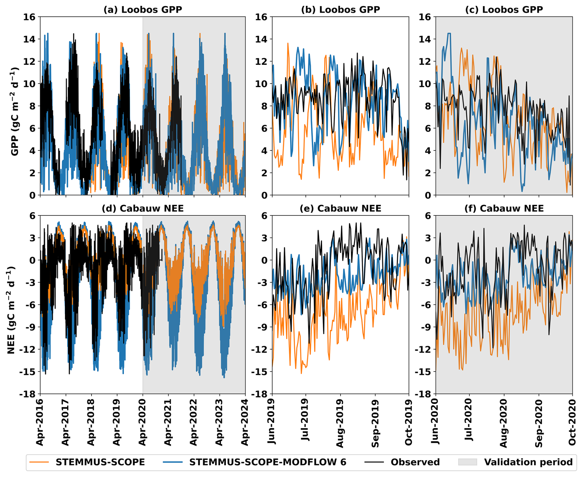
Figure 7 Comparison of daily simulated carbon fluxes, i.e. gross primary productivity (GPP) and net ecosystem exchange (NEE) values by STEMMUS-SCOPE (orange lines), by STEMMUS-SCOPE-MODFLOW 6 (blue lines), and observed ones (black lines) during the calibration period (1 April 2016–31 March 2020) and the validation period (1 April 2020–31 March 2024; grey shaded) at: (a) Loobos, and (d) Cabauw; with windows zooming (b, e) in a dry period example in the calibration period (1 June–30 September 2019), and (c, f) in a dry period example in the validation period (1 June–30 September 2020).

Figure 8 shows half-hourly observations and simulated SIF from ST-SC and ST-SC-MF6 on certain days at Cabauw, when the observed SIF data were available. During the summer days 9–14 August 2022 (Fig. 8a), the ST-SC-MF6 demonstrated a better agreement with the SIF observations as compared to the ST-SC. Both models aligned well with the observations during the summer days 3–6 June 2023 (Fig. 8c), which were dry days (Fig. 4c and d), while both models underestimated the SIF on the winter days 12–15 November 2022 (Fig. 8b).

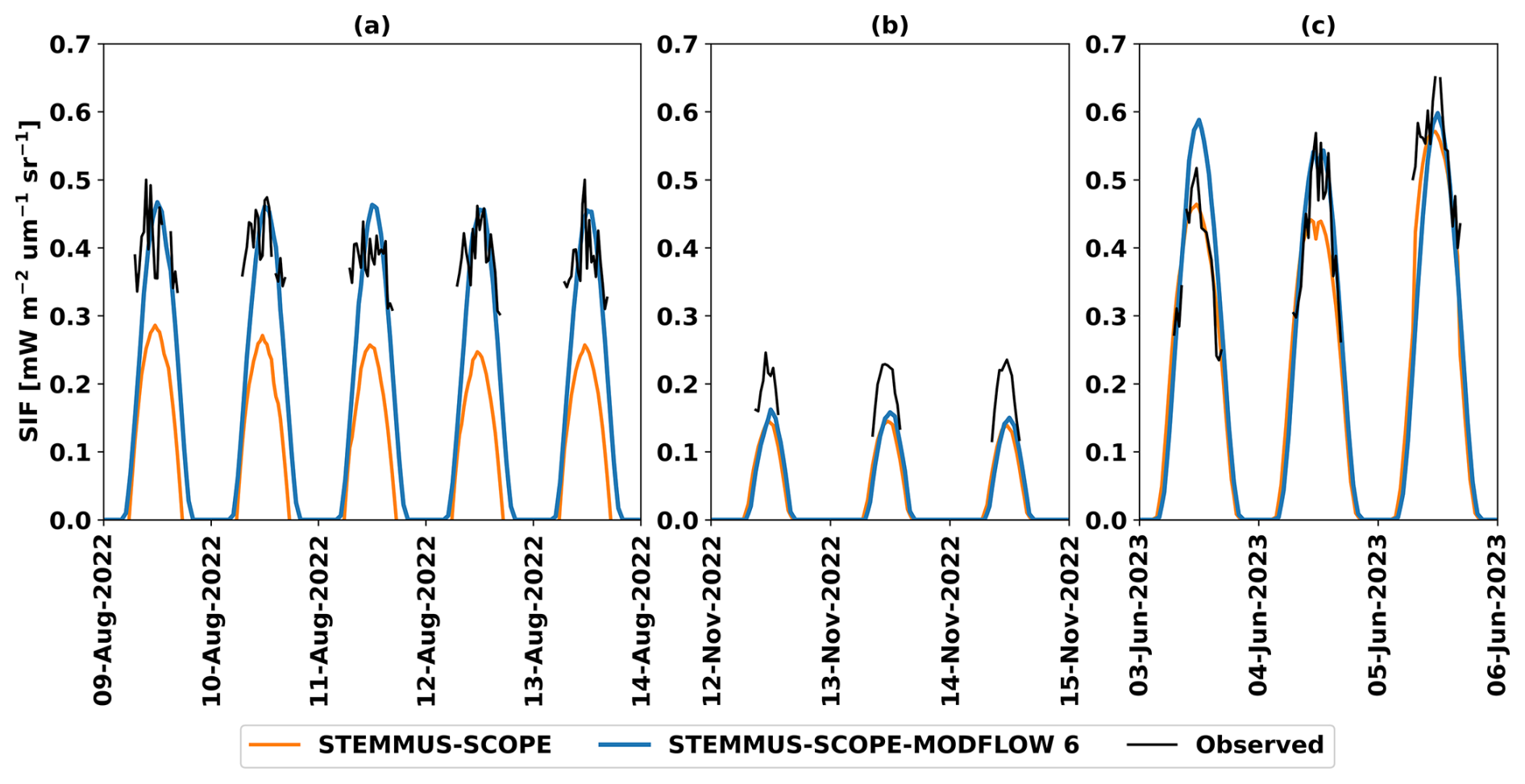
Figure 8 Cabauw site – comparison of half-hourly simulated sun-induced chlorophyll fluorescence (SIF) by STEMMUS-SCOPE (orange lines), by STEMMUS-SCOPE-MODFLOW 6 (blue lines), and observed ones (black lines) during the days: (a) 9–14 August 2022, (b) 12–15 November 2022, and (c) 3–6 June 2023.

4 Discussion

The ST-SC-MF6 IEM was tested at three different sites (the Loobos forest, the Cabauw and Veenkampen meadow sites) in the Netherlands. Different key variables from the water, energy, and carbon cycles were analyzed for the two simulations (with and without coupling with MODFLOW 6) – namely, θ, T_s, GWL, GT, ET, GPP, NEE, and SIF. The AIC evaluation confirmed that the added model complexity of ST-SC-MF6 is strongly justified by its enhanced predictive accuracy across all study sites. The benefits of representing the groundwater in modelling the SPAC processes are described in the following subsections.

4.1 Effect of groundwater on soil moisture

The benefits obtained from incorporating groundwater within ST-SC-MF6 come from the role changes that groundwater plays in the processes simulation. The GWL, simulated by MODFLOW 6, was used as a bottom boundary for the soil water module in STEMMUS-SCOPE, thereby influencing the ψ_s,i and θ profiles. In the capillary fringe zone, above the GWL, soil is nearly saturated, causing the ψ_s,i to become less negative, and the corresponding θ to increase significantly. Moving upward to the soil surface, the influence of the GWL gradually diminishes, and other surface forces (e.g., precipitation) become the dominant driver of ψ_s,i and θ in the upper soil layers. However, the extent to which the GWL affects ψ_s,i and θ depends on the thickness of the unsaturated zone, where groundwater fluctuations occur. When the water table is shallow, its influence can extend upward beyond the lower soil layers, affecting the upper profile with decreasing intensity. Then, over time, as GWL rises, the entire ψ_s,i profile shifts towards less negative and θ increases throughout the entire soil profile. Conversely, a falling GWL leads to a more negative ψ_s,i profile and a decrease in θ.

The impact of groundwater on the θ profile was particularly evident at Cabauw and Veenkampen sites, where groundwater depths were shallow (from 0 to 1.25 m b.l.s.). At these two sites, the strong hydraulic connectivity between the phreatic surface and the unsaturated zone enabled the GWL fluctuations to propagate upward through the soil profile, directly regulating the θ dynamics. The ST-SC-MF6 models improved the representation of the seasonal θ variability by dynamically resolving this connectivity. During winter wet periods (December–March), the θ variability is primarily controlled by groundwater fluctuations (McMillan and Srinivasan, 2015). This was observed in the simulations by the rise of the GWL (Fig. 3c and d), associated with the increase of the θ towards the observed θ peaks (0.6 m³ m⁻³ at Cabauw and 0.75 m³ m⁻³ at Veenkampen), approaching near-saturation conditions (Fig. 4c, d, e and f). In spring periods (April–June), when vegetation is mainly active, enhanced RWU_s progressively depletes the θ, while GWL is still relatively high. Further towards summer dry periods (June–September), limited or no precipitation reduced the R_g, leading to GWL decline and the development of a drier soil profile (Gao et al., 2017; Li et al., 2017) with minimum θ values of 0.2 m³ m⁻³ at Cabauw and 0.15 m³ m⁻³ at Veenkampen, respectively (Fig. 4c, d, e and f).

At the Loobos site, the GWL impact on the θ profile was not evident. This can be attributed to two main factors. First, the site is characterized by a loamy sandy soil with a relatively low maximum observed θ (∼ 0.16 m³ m⁻³) along the entire profile (Fig. 4a and b), indicating limited soil water holding capacity. Second, the groundwater depth was relatively moderate (3.0–5.0 m b.l.s.), as compared to the other two sites. However, whether groundwater influence becomes negligible at depths between 3 and 5 m cannot be generalized from the Loobos site alone. An experimental study by Zhao et al. (2023), conducted in a semi-arid region, showed that the θ within the upper 2 m of sandy soil increased with soil depth at 6 and 10 m groundwater depths, whereas there was no significant impact on θ at groundwater depth of 15 m. These findings, unlike the case in Loobos, suggest that the extent of the critical groundwater depth, which can still influence θ is site-dependent and strongly controlled by soil hydraulic properties. Therefore, future testing at different sites with similar groundwater depths (3 to 5 m) or even deeper, but different soil characteristics than the Loobos site is further required. Nevertheless, the ST-SC models at the three sites were unable to reproduce the observed amplitude and seasonal variability of θ (Fig. 4). This is because the absence of dynamic groundwater feedback prevented realistic representation of key interacting groundwater processes, i.e. R_g, RWU_s and RWU_g and their combined influence on θ.

4.2 Effect of groundwater on soil temperature

Groundwater energy and mass, represented by GWL and GT, showed effects on the T_s as discussed in the following subsections.

4.2.1 Effect of groundwater temperature on soil temperature

The GT, simulated by MODFLOW 6, was used as a bottom boundary for the STEMMUS-SCOPE soil energy module. At Loobos, where GT observations were available, the ST-SC-MF6 produced a better simulation of the T_s profile as compared to the ST-SC (Fig. 5a and b). At this site, the groundwater depth is relatively moderate (3.0–5.0 m b.l.s.), resulting in a balance between atmospheric and groundwater heat processes' influence on T_s. While the shallower soil layers closely follow atmospheric conditions, deeper layers are more influenced by groundwater conditions (Parrales et al., 2026). Both observed and simulated GT fluctuated between 10.6 °C during winter periods and 9.8 °C during summer periods (Fig. 3b). In contrast, T_s exhibited a much larger seasonal variability (Fig. 5a and b), with both observed and simulated T_s ranging from 15.0–18.0 °C during summer period to 5.0–8.0 °C during winter period across the soil profile. With increasing soil depth, the T_s is damped with a seasonal phase lag until gradually approaching stable GT values. By incorporating the simulated GT as a bottom boundary condition for the unsaturated zone, the ST-SC-MF6 simulation successfully reproduced the same patterns as the observed T_s. During winter periods, the GT was higher than T_s, generating upward heat transfer by diffusion, i.e. temperature gradient, from the saturated to the unsaturated zone. Towards the spring period (April–June), GT gradually declined, while T_s increased, resulting in a temporary equilibrium state between the two thermal regimes. Later during summer periods, the opposite situation occurs, with T_s exceeding GT, reversing the direction of the heat transfer from the unsaturated to the saturated zone.

It is notable that matching the simulated T_s with the corresponding observations at the Loobos site was challenging. The Loobos site has low values of θ (maximum value = 0.16 m³ m⁻³) along the soil profile (Fig. 4a and b), corresponding with relatively low T_s values (maximum value = 18.0 °C). Such a situation created extra difficulty in modelling, since in STEMMUS-SCOPE, the θ and T_s are simulated together with many influencing factors as follows: (1) the low θ may shift the energy partitioning to more sensible heat and less latent heat, which leads to low values of evaporation and extra soil warming (overestimation of T_s profile); and (2) the thermal parameterization (K_T and c_s) in STEMMUS-SCOPE follows the de Vries formulation (Yu et al., 2018), which is influenced by θ. In this case, the low θ values lowered the values of thermal parameters, which may lead to rapid soil heating and further contribute to the overestimation of T_s. Hence, the overestimation of the θ amplitude by ST-SC dampened the amplitude of the T_s.

4.2.2 Effect of groundwater level on soil temperature

At Cabauw and Veenkampen, although no GT observations were available to control the simulations, groundwater still exerted potential influence on T_s profile, driven by the GWL rather than the GT. The shallow groundwater depths (0–1.25 m b.l.s.) at these two sites enhanced soil thermal conductance and heat capacity, which facilitated heat transfer between the topsoil and the subsurface (Alkhaier et al., 2012). Under such conditions, the unsaturated zone becomes more thermally connected to the atmospheric forcing rather than the saturated zone. Previous studies have reported a strong correlation between GWL and T_s, particularly under shallow groundwater depths, i.e. < 5.0 m (Alkhaier et al., 2012; Malik et al., 2021; Mandal and Roy, 2024; Oishy et al., 2025). The de Vries heat transport formulation, implemented in the energy module of STEMMUS-SCOPE (Yu et al., 2018), allows for producing such GWL–T_s relationship.

At Cabauw, the ST-SC-MF6 model showed a better simulation of the T_s profile as compared to the ST-SC model (Fig. 5c and d). During winter periods, the GWL rose (Fig. 3c), which was associated with high θ values, i.e. 0.6 m³ m⁻³ (Fig. 4c and d), nearly approaching saturation, and relatively low T_s (Fig. 5c and d). Nevertheless, both θ and T_s of the ST-SC-MF6 remained higher than the ones, produced by the ST-SC model and closer to the observed ones. During summer periods, the GWL declined, leading to low θ and high T_s values, while T_s remained higher than the values produced by the ST-SC model. Collectively, during the hydrological year, the presence of the shallow GWL in the ST-SC-MF6 simulation increased the seasonal amplitude of θ, i.e. raising maximum θ during winter while maintaining nearly similar minimum θ in summer. This behaviour, in turn, reduced the seasonal amplitude of T_s, i.e. increasing minimum T_s during winter and reducing maximum T_s during summer. In contrast, the ST-SC model, due to the absence of GWL, underestimated the θ amplitude and consequently overestimated the T_s amplitude.

At Veenkampen, the GWL showed little impact on the T_s simulation (Fig. 5e and f), although the ST-SC-MF6 model improved the θ simulation by raising the θ level, particularly the winter peaks, relative to the ST-SC model, whose θ showed a similar amplitude but was systematically lower (Fig. 4e and f). This shift in θ did not noticeably affect the thermal properties of the soil, which remained similar in both simulations, leading to comparable T_s dynamics. Additionally, in both models, the amplitude of the simulated T_s was slightly overestimated. The likely reason is the resistance scheme in the soil energy module in STEMMUS-SCOPE, which follows the big leaf concept, assuming that the boundary layer resistance is the same for all canopy layers – a simplification that could be refined in the future.

4.2.3 Effect of groundwater on surface soil temperature and canopy temperature

Beyond the groundwater influence on T_s dynamics, groundwater can also affect the thermal regime of the land surface and vegetation canopy. These effects may propagate upward, influencing surface soil temperature (T_ss) and canopy temperature (T_c), which in turn regulate vegetation physiological processes such as stomatal conductance and carbon assimilation.

At Loobos, the groundwater – soil heat exchanges, simulated by the ST-SC-MF6 model, facilitated proper simulation of temperature-dependent processes within the SPAC. In particular, GT played a crucial role in cooling T_s, especially in the deeper soil layers, close to the capillary fringe zone, thereby stabilizing the root-zone thermal conditions and supporting the RWU_g – as observed through the increase of RWU_g, simulated by ST-SC-MF6 (Sect. 4.3.3). Furthermore, the moderating influence of the GT on the T_s propagated upward to cool down T_ss and T_c. The ST-SC-MF6 simulation produced consistently cooler T_ss and T_c (i.e. lower peaks) during the spring periods compared to the ST-SC simulation, with reductions of approximately 1 °C in T_ss (Fig. 9a and b) and up to 2 °C in T_c (Fig. 9c and d).

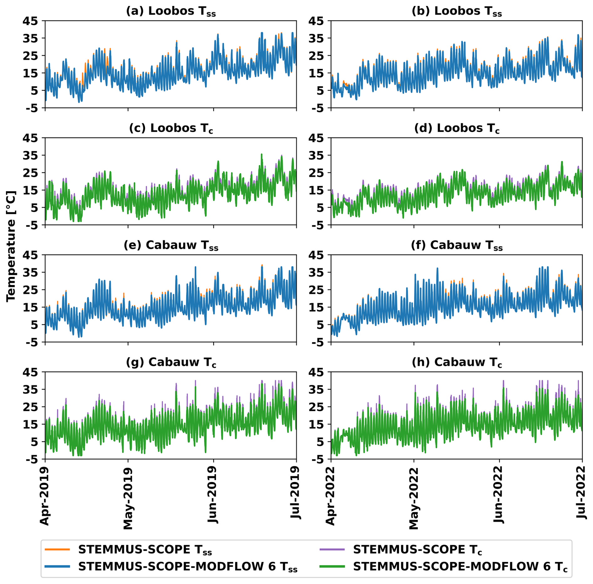
Figure 9 Comparison of half-hourly simulated surface soil temperature (T_ss) by STEMMUS-SCOPE (orange lines), by STEMMUS-SCOPE-MODFLOW 6 (blue lines), simulated canopy temperature (T_c) by STEMMUS-SCOPE (purple lines), by STEMMUS-SCOPE-MODFLOW 6 (green lines) in a spring period example in the calibration period (1 April–30 June 2019) for Loobos (a, c) and Cabauw (e, g), and in the validation period (1 April–30 June 2022) for Loobos (b, d) and Cabauw (f, h).

At Cabauw, the influence of groundwater on the surface thermal regime is primarily controlled by the shallow GWL rather than GT. The shallow GWL moderates near-surface thermal conditions through its control on θ and thermal properties, enhancing the buffering of temperature fluctuations in the soil profile. The ST-SC-MF6 simulation produced cooler T_ss (i.e. lower peaks, Fig. 9e and f) and T_c (Fig. 9g and h) during the spring periods as compared to the ST-SC simulation, with average reductions of about 1 and 2 °C, respectively. Such moderation of T_c, particularly during the spring periods, when the vegetation activity is high, would maintain stomatal conductance and support carbon uptake. Under good nutrient and water availability conditions, slightly cooler T_ss and T_c would further enhance photosynthesis and carbon assimilation (Oishy et al., 2025), as observed in the NEE, simulated by ST-SC-MF6 (Sect. 4.4).

4.3 Effect of groundwater on evapotranspiration components

The explicit representation of groundwater improved the simulation of ET. As shown in Fig. 6, the ST-SC-MF6 simulations generally reproduced the observed ET dynamics better than the ST-SC simulations, particularly during dry periods when groundwater contributed to sustaining θ and RWU. The improved ET representation originates from the more realistic simulation of individual ET components, i.e. E_ss, RWU_s, and RWU_g, which are discussed below.

4.3.1 Subsurface evaporation

At Cabauw and Veenkampen, the E_ss values simulated by ST-SC-MF6 models were increased by 7.3 % and 12.6 %, respectively, as compared to the ST-SC models. These increases can be attributed to two mechanisms. First, the formation of the capillary fringe zone (Fig. 1) above the phreatic surface enabled the calculation of the Cap flux. The Cap flux further contributed to the water loss that moved upward to the land surface, where E_ss takes place (Hird and Bolton, 2017; Balugani et al., 2021, 2023). Second, the improved simulation of ψ_s,i and the corresponding θ created strong upward hydraulic gradients that promoted E_ss (Huo et al., 2020). Both experimental (Huo et al., 2020) and field studies (Yang et al., 2021b) have demonstrated that shallow groundwater, i.e. generally less than 2.5 m, can sustain evaporation by maintaining moisture supply to the soil layers.

4.3.2 Root soil water uptake

The inclusion of GWL as a dynamic bottom boundary has improved the simulation of the ψ_s,i across the soil profile by allowing proper seasonal dynamics of ψ_s,i with respect to the GWL fluctuations. The improved representation of ψ_s,i resulted in a substantial improvement of the RWU_s by better capturing the hydraulic connectivity between the saturated zone and the root zone (Wang et al., 2023). At Cabauw and Veenkampen, RWU_s, which is based on ψ_s,i (Eq. 5), was increased by 29.6 % and 35.9 %, respectively. Such improvement highlights the sensitivity of the RWU_s to the groundwater depth, particularly when the groundwater depth lies within the range of 0.5–2.5 m from the land surface, as reported by Sulis et al. (2017). They demonstrated using two different models, i.e. TerrSysMP (Shrestha et al., 2014) and ParFlow-WRF (Maxwell et al., 2011), applied at vegetated areas in the Rur catchment in Germany, that the GWL fluctuations significantly influence the energy fluxes, further affecting the RWU_s, through their impacts on the θ profile. This mechanism has been described by Huang et al. (2017), who showed that shallow groundwater can: (a) prevent the ψ_l from declining to the critical ψ_l that triggers stomatal closure; and (b) maintain high values of ψ_s,i, thereby preventing the rapid depletion of the θ. Consequently, these processes led to increasing the plant water storage and supported high RWU_s, as has been observed in the ST-SC-MF6 simulations at Cabauw and Veenkampen sites.

4.3.3 Root groundwater uptake

The ψ_g,i was explicitly defined for the soil layers below the capillary fringe zone, which was further used to calculate RWU_g (Eq. 6). The RWU_g is an additional component that contributed 28.0 %, 15.2 %, 13.0 % to the total ET at the three sites (Loobos, Cabauw, and Veenkampen), respectively.

At Loobos, the d_max of the evergreen forest was defined in the models as 4.0 m, allowing the plant roots to access the groundwater, located at depths between 3.0 and 5.0 m b.l.s. The increase in the RWU originated mainly from the RWU_g, while RWU_s showed nearly no change. This is because of the similar θ simulation by both ST-SC and ST-SC-MF6 models, resulting in comparable RWU_s estimates. Furthermore, the groundwater contribution to ET was more significant during dry periods (Fig. 6b and c), when θ was depleted owing to lack of rain, while the GWL continued to support the water uptake by plant roots. Such a mechanism has been reported in many previous studies (Zhu et al., 2009; Wang et al., 2023; Du et al., 2025). From a modelling perspective, Bieri et al. (2025) also showed that the failure of the models to reproduce proper dry season transpiration is often related to the absence of deep RWU mechanisms in the simulations. Moreover, the impacts of GT (discussed in Sect. 4.2.1) on cooling the T_s for the deeper soil layers, allowed for better RWU_g during spring and summer periods.

At Cabauw and Veenkampen, the d_max of the grassland was set to 0.5 m in the models, allowing the roots to access the groundwater, which fluctuated between 0 and 1.25 m b.l.s. However, the contribution of RWU_g to the total ET at these two sites remained smaller than at Loobos. That is because the soil water availability, reflected in the improved simulation of θ by the ST-SC-MF6 models, was sufficient to sustain higher RWU_s, thereby reducing the reliance on the RWU_g. In such shallow water table conditions, land surface processes, including RWU, are subject to more energy control rather than water control (Wang et al., 2023).

4.4 Effect of groundwater on carbon fluxes and SIF

Explicit representation of groundwater in the IEM also had an impact on the carbon fluxes (GPP and NEE), particularly during dry periods (Ruehr et al., 2023), even though groundwater is not explicitly represented in the carbon fluxes' calculations. Instead, θ, which is dynamically constrained by GWL, is included in the carbon fluxes' calculations and is positively correlated with carbon fluxes through affecting plant water status and stomatal conductance. When θ is limited (i.e., low water content), both ψ_s,i and ψ_l decreased (became more negative), and the gradient between the ψ_s,i and ψ_l shifted to more negative. Under such conditions, the plant closed the stomata, so the stomatal conductance decreased in an attempt to mitigate water stress, reducing CO₂ uptake and consequently lowering GPP and NEE. In contrast, higher θ increased the stomatal conductance, leading to higher CO₂ uptake, promoting carbon assimilation and higher GPP and NEE.

At Cabauw, where GWL is relatively shallow, exerting strong control on the θ dynamics, the ST-SC-MF6 showed improved simulation of both θ and NEE, as compared to the ST-SC model. In particular, the NEE was increased during the dry periods (Fig. 7e and f), due to enhancement in the simulated θ, resulting from the dynamically updated GWL values. This simulated mechanism aligns with recent findings that groundwater depth is a critical control on ecosystem productivity, with higher carbon assimilation occurring under shallow groundwater conditions (Glanville et al., 2023). Specifically, in meadow ecosystems with shallow GWL, such as in Cabauw, shallow groundwater can enhance net carbon uptake by suppressing soil respiration under near-saturated soil conditions, thereby increasing the net ecosystem carbon sink, as discussed by Sun et al. (2021). Their analysis, in two meadow sites in the Tibetan Plateau in China, revealed that the influence of high θ, maintained by shallow GWL, played a more significant role in controlling carbon fluxes, rather than low temperature. Moreover, the pronounced improvement of the simulated NEE during the dry periods (Fig. 7e and f) is consistent with the evidence that there is a significant positive correlation between groundwater depth and carbon fluxes under certain conditions, i.e. during dry periods when vegetation activity is minimum, and carbon fluxes have low values (Koirala et al., 2017).

Whereas, at Loobos, there was negligible GWL effect on the simulated θ and consequently also on the simulated GPP (Fig. 7b and c). This is because: (a) the simulated GWL was relatively moderate (3.0–5.0 m), limiting its hydraulic connection to the unsaturated zone, consistent with the observation that deeper GWL reduces carbon fluxes (Glanville et al., 2023); and (b) the maximum observed θ was generally low (0.16 m³ m⁻³), indicating low water availability for vegetation, and consequently poor carbon assimilation.

The contrasting responses between Loobos (no GPP improvement) and Cabauw (NEE improvement) demonstrate that groundwater effects on carbon cycling and vegetation productivity are strongly site-dependent. Specifically, the groundwater influence becomes significant when the water table is shallow enough to interact with the root zone and meaningfully affect θ dynamics. These findings support recent calls to explicitly represent groundwater–carbon feedbacks in Earth system models to improve predictions of carbon fluxes under environmental change (Klaus, 2023). Moreover, it was highlighted by Tak et al. (2023) regarding the importance of groundwater level management to optimize ecosystem carbon uptake.

Similarly, in the SIF simulation, the impact of groundwater was evident at the Cabauw site through the changes in θ. The θ affects water availability to the plant, which regulates stomatal conductance and photosynthetic activity, and in turn contributes directly to the SIF calculations. The simulated SIF was enhanced on the dry summer days 9–14 August 2022 (Fig. 8a) due to the enhanced θ, caused by shallow GWL. Meanwhile, groundwater had no clear impact on the simulated θ during the summer days 3–6 June 2023 (Fig. 8c), since, during those days, both ST-SC and ST-SC-MF6 produced a very similar θ simulation (Fig. 4c and d), resulting in no groundwater impact on the SIF simulation. Besides, both models underestimated the SIF on the winter days 12–15 November 2022 (Fig. 8b), likely due to other parameters and/or forces that could influence the SIF calculations, which are beyond the scope of this study and need further investigation.

4.5 Recommendations

The changes in the θ, T_s, ET, GPP, NEE, and SIF variables suggest that accounting for groundwater interactions significantly improves the model's ability to represent the SPAC. However, certain assumptions and/or limitations highlight areas for future development. The coupling between STEMMUS-SCOPE and MODFLOW 6 was applied to three sites in the Netherlands, and only for 1D vertical flow. Future efforts would include expanding the ST-SC-MF6 IEM to 2D or 3D scale and incorporating groundwater lateral flow and surface runoff to support broader climate-resilience evaluations and decision-support applications (Samper et al., 2025). In addition, while the three presented applications focused on shallow-to-moderate groundwater depths (0–5.0 m), applying the developed IEM framework to deeper groundwater systems would present another valuable avenue for future research. Furthermore, although calibration was performed manually in this proof-of-concept study, future work should incorporate a multi-objective automatic calibration framework to systematically reduce parameter uncertainty and enhance model robustness. Implementing such an approach in future 2D/3D applications will increase confidence in predictive simulations and strengthen the broader applicability of the developed IEM. Moreover, the inconsistency in the amplitude of the simulated T_s (i.e., higher peaks or lower troughs than observations) could be addressed by improving the boundary layer resistance scheme in STEMMUS-SCOPE. Additionally, the incorporation of a more physically based simulation of SIF is expected to better capture the SIF dynamics, especially during winter periods.

5 Conclusions

This study demonstrated the added value of incorporating the groundwater component in SPAC modelling by coupling the STEMMUS-SCOPE SPAC model with the MODFLOW 6 IHM, resulting in the ST-SC-MF6 IEM. Results from 1D applications at three sites in the Netherlands (Loobos, Cabauw, and Veenkampen) indicated that explicitly including groundwater (mass and energy) improves the simulation of key ecohydrological variables. The θ improvement was largest at sites with shallow groundwater depths (0–1.25 m b.l.s.; Cabauw and Veenkampen), particularly during wet periods, when the dynamic GWL allowed the soil profile to approach saturation. This improved θ further propagated to the thermal regime, namely the T_s and T_c dynamics, through the θ-dependence of the thermal properties. In contrast, at Loobos, where the θ effect was minor, the simulation of T_s improved because GT provided a stable lower thermal boundary. ET was also improved by groundwater contributions, particularly during dry periods, either through the improved simulation of ψ_s,i and the corresponding θ, which further enhanced E_ss and RWU_s at Cabauw and Veenkampen, or directly through the increased RWU_g at Loobos. At Cabauw, the improved θ, sustained by the dynamic GWL, led to improved simulation of carbon uptake (NEE) and SIF. Notably, groundwater impacts on GPP were limited at Loobos, due to its low soil water holding capacity, corresponding with minor impacts of GWL on θ, and the relatively moderate groundwater depths (3.0–5.0 m b.l.s.). Overall, groundwater showed different effects on the analyzed variables among the three sites. These differences emphasize that the impact of groundwater on the SPAC is strongly site-dependent and that the vegetation–groundwater interactions are controlled by groundwater depth, soil properties, plant species and rooting characteristics. In conclusion, this study demonstrates that explicitly including groundwater dynamics in SPAC modelling is essential for realistically simulating ecosystem water, energy, and carbon cycles.

Appendix A: List of symbols

α	Alpha coefficient of Van Genuchten equation
a.s.l.	Above sea level
AIC	Akaike Information Criterion
b.l.s.	Below land surface
BMI	Basic model interface
Cap	Capillary rise flux
cs	Specific heat capacity of solids
dmax	Maximum rooting depth
DTa	Transport coefficient of the adsorbed liquid flow due to temperature gradient
Dvh	Isothermal vapour conductivity
DvT	Thermal vapour diffusion coefficient
Ess	Subsurface evaporation
ET	Evapotranspiration
GPP	Gross primary productivity
GT	Groundwater temperature
GWE	Groundwater energy
GWF	Groundwater flow
GWL	Groundwater level
IEM	Integrated ecohydrological model
IHM	Integrated hydrological model
K	Unsaturated hydraulic conductivity
KGE	Kling–Gupta efficiency
Kh	Horizontal hydraulic conductivity
Ksat	Vertical saturated hydraulic conductivity
KT	Thermal conductivity of solids
Kv	Vertical hydraulic conductivity
LAI	Leaf area index
LSM	Land surface model
n	n coefficient of Van Genuchten equation
NEE	Net ecosystem exchange
ψg,i	Groundwater potential of layer i
ψl	Leaf water potential
ψs,i	Soil water potential of layer i
Q	Calculated flux to be either recharge (Rg) or capillary rise flux (Cap)
Qheat	Heat flux above water table
qLh	Soil liquid water flux driven by soil matric potential gradient
qLT	Soil liquid water flux driven by temperature gradient
qvh	Soil water vapour flux driven by soil matric potential gradient
qvT	Soil water vapour flux driven by temperature gradient
ρL	Density of liquid water
ρs	Bulk density of solids

ρv	Density of water vapour
Rg	Groundwater gross recharge
RMSE	Root mean square error
Rn	Groundwater net recharge
rr,i	Root resistance to water flow radially across the roots
RS	Remote sensing
rs,i	Soil hydraulic resistance
RTn	Groundwater Net recharge temperature
RWU	Root water uptake
RWUg	Root groundwater uptake
RWUs	Root soil water uptake
rx,i	Plant's axial resistance to flow from the root xylem to the leaves
S	Sink term in Richards equation
SIF	Sun-induced chlorophyll fluorescence
SPAC	Soil-plant-atmosphere continuum
Ss	Specific storage
ST-SC	STEMMUS-SCOPE
ST-SC-MF6	STEMMUS-SCOPE-MODFLOW 6
Sy	Specific yield
θ	Soil moisture (volumetric water content)
θL	Soil liquid volumetric water content
θr	Residual water content
θs	Saturated water content
θv	Soil vapour volumetric water content
Tc	Canopy temperature
Ts	Soil temperature
Tss	Surface soil temperature