Improving weather radar rainfall estimates by merging with commercial microwave link data: a fully reproducible, large-scale method intercomparison

Accurate rainfall estimation is essential for hydrometeorological applications, but capturing the fine spatiotemporal variability of rainfall remains challenging. In this study, we assess the impact of merging commercial microwave link (CML) data with weather radar for quantitative precipitation estimation (QPE) using two openly available datasets with contrasting observational densities. We compare multiple merging methods, including kriging with external drift (KED), and derive a block kriging interpolation method to account for the line-average nature of CMLs. The results show that merging CML data improves radar QPE, with reductions in mean absolute error (MAE) of up to 41 % for multiplicative merging and up to 38 % for KED, aligning well with similar studies using rain gauges. Performance depends on rainfall intensity, distance, and network density: in sparse networks, multiplicative methods yield the lowest RMSE and MAE, indicating that radar errors are dominated by scaling errors, though KED and additive methods maintain slightly higher spatial correlation (PCC) over distance. In dense networks, all methods perform comparably. Overall, additive methods perform best at capturing extremes. Despite accounting for line-averaging, block kriging performed similarly to point-based kriging. All merging methods reduced RMSE and MAE compared to unadjusted radar fields. The merging framework and intercomparison study are openly available, enabling reproducibility and further exploration by the scientific community.

1 Introduction

Accurate rainfall estimation is important for many hydrometeorlogical applications like flood forecasting, urban drainage design, or water-resources management. However, rainfall is highly intermitted both in space and time and capturing this variability remains one of the main challenges in hydrometeorology, particularly during convective events. Even dense observational networks consisting of rain gauges and weather radars struggle to correctly resolve the often fine grained spatio-temporal variability of rainfall (Cristiano et al., 2017; Rombeek et al., 2025; Schleiss et al., 2020).

Rain gauges provide relatively precise point measurements and are considered as the traditional reference for quantitative precipitation estimation (QPE). Yet, their spatial density is typically insufficient to represent the full variability of rainfall at kilometer or sub-kilometer scales (O and Foelsche, 2019; Hänsler and Weiler, 2022). This limitation persists even in well-instrumented regions e.g. with one rain gauge for roughly every 200–400 km² in Central Europe, and it becomes critical in areas where the observational infrastructure is sparse. Consequently, radar observations have become more widely used for providing high-resolution areal rainfall information due to high resolution. Despite these advantages, weather radar rainfall estimates remain affected by multiple error sources, including attenuation, beam blockage, vertical profile effects, calibration drifts, and the presence of the melting layer which are partially but not completely resolved by the use of dual-pol radars (Aldana et al., 2025; Schleiss et al., 2020; Hänsler and Weiler, 2022). These uncertainties limit the accuracy of radar-only QPE and motivate the merging of radar data with ground-based observational data.

Commercial microwave links (CMLs) based on the the opportunistic use of attenuation data from cellular communication networks have emerged over the past decade as a robust source of rainfall information. Specifically, rainfall intensity R (mm h⁻¹) is derived from the average rain-induced attenuation k (dB km⁻¹) via the power-law relationship R=a k^b, assuming uniform liquid precipitation along the path. The parameters a and b depend on the link's frequency and polarization. Estimating precipitation from commercial microwave links offers several key advantages. Unlike radar, the power law relating precipitation to induced attenuation is less sensitive to the raindrop size distribution (Chwala and Kunstmann, 2019), thus providing a more robust relationship than the one between rainfall intensity and radar reflectivity. Furthermore, CMLs provide an estimate of path-averaged precipitation, resulting in a product with greater spatial representativeness than a point-based rain gauge, as well as measurements taken close to the ground (unlike weather radar). Conversely, one of the main limitations remains instrument sensitivity, defined by signal quantization, path length, and frequency, which are characteristics not always optimized for using the infrastructure as a precipitation sensor. Despite these limitations, numerous studies have shown that path-averaged rain-induced attenuation along CMLs can be converted into accurate QPE, in particular for moderate and heavy precipitation (Chwala and Kunstmann, 2019; Uijlenhoet et al., 2018; Messer and Sendik, 2015). In Europe, CMLs are increasingly regarded as a complementary data source for rainfall (Olsson et al., 2025), while in data-sparse regions such as parts of Africa, they can serve as a quasi-independent measurement system (Blettner et al., 2025; Djibo et al., 2023; Overeem et al., 2021). One particularity of CML data is that, unlike weather radar or rain gauge observations, it is not owned by national or local authorities. As a consequence, CML data is generally restricted to the individual research groups that obtained it and does not, for example in the EU, fall under open-data policies. Only recently have the first larger CML datasets become publicly available (Andersson et al., 2022; Covi and Roversi, 2025; Overeem et al., 2024c).

Merging has been extensively studied in the literature (Jewell and Gaussiat, 2015; Delrieu et al., 2014; Overeem et al., 2024b), and there are many methods for doing this. For instance, Goudenhoofdt and Delobbe (2009) merged weather radar with a dense rain gauge network in Belgium. They found that merging methods that allowed the radar correction to vary spatially, performed better than applying a mean correction to the entire rainfall field. This finding was supported by Nielsen et al. (2024), who merged radar with personal weather station (PWS) and CML data, and found that a localized median correction dampened the effect of outliers. Sideris et al. (2014) added a temporal component to the merging process, allowing the previous timestep to influence the current time step. They found that the proposed method offered advantages over existing methods, particularly in areas where sparse rain-gauge coverage, measurement errors, or high variability compromise the stability of traditional geostatistical methods.

Although Nielsen et al. (2024) utilized CMLs in their study, these were combined with a much larger number of PWSs, making it difficult to assess the impact of CMLs on radar merging performance. Moreover, their merging method used the midpoint of the CMLs to represent its location, which may be suboptimal given that CMLs represent a path averages.

In this work we assess the impact of merging data from CMLs with weather radar data using two existing large openly available datasets featuring contrasting observational densities. We investigate different merging paradigms, each representing a distinct physical hypothesis from the literature regarding radar error structures. Specifically, additive merging assumes radar errors act as spatially varying offsets (e.g., range degradation or beam blockage), multiplicative merging assumes errors scale with rainfall intensity (e.g., Z–R parameter mismatch), and Kriging with External Drift (KED) assumes errors consist of a combination of both offset and scaling mechanisms by modeling the radar as a linear spatial trend. Furthermore, we evaluate spatial interpolation geometries, including block kriging, which explicitly accounts for the line geometry of the CMLs.

The merging methods and intercomparison study are implemented in mergeplg (Øydvin et al., 2026a) and made openly available and fully reproducible (Covi et al., 2026a), allowing the scientific community to experiment and contribute. Through this framework, we seek to answer three research questions: First, how much does merging CML data with weather radar improve QPE accuracy compared to raw, unadjusted radar when evaluated against independent rain gauge observations? Second, what do the relative performances of additive, multiplicative, and external drift paradigms reveal about radar error structures? Third, how do spatial interpolation geometries (point vs. block kriging) and geostatistical choices influence merging performance across contrasting sparse and dense CML networks?

2 Datasets

We use two open CML datasets that are accompanied by radar and rain gauge data as reference. The first is the OpenMRG dataset covering the Gothenburg region, Sweden, from June to August 2015 (Andersson et al., 2022). The datasets includes measurements from 364 CMLs, spanning about 2800 km² (1 CML per 7.7 km²), with the majority of the CMLs located in the city center (Fig. 1a). Each CML comprise two sublinks. Signal levels – both transmitted (TSL) and received (RSL) – were recorded every 10 s and resampled to 1 min intervals by retaining the first value in each period. The signal levels have a quantization of approximately 0.1 dB. The CMLs are operated across a frequency range of 7 to 38 GHz, with the majority exceeding 25 GHz as shown in Fig. 1c). All variables exhibit high data availability, with 97.3 % of CMLs, 99.1 % of radar measurements, and 100 % of rain gauge data present. The reference data consists of one gauge from SMHI and ten municipality rain gauges with 15 min resolution, as well as a radar reflectivity composite from the three nearest SMHI weather radar with a 2 km and 5 min resolution. The reflectivity values are transformed to rainfall values using the standard Marshall–Palmer Z–R relation (Marshall and Palmer, 1948).

The second dataset is OpenRainER, covering the Emilia-Romagna region in Italy for the years 2021 and 2022 (Covi and Roversi, 2025; Covi et al., 2026b). We use three months of data from June to August 2022. The dataset includes measurements from 153 CMLs, spanning about 21 000 km² (1 CML per 137 km²), with most CMLs located along the mountainous region in the south (Fig. 1b). TSL and RSL were recorded instantaneously with a resolution of 1 min. The signal levels appear to have an underlying quantization of approximately 1 dB, with intermediate values in the data likely arising from temporal averaging. Frequencies range between 24.6 to 25.6 GHz (Fig. 1d). Compared to OpenMRG, the data availability is slightly lower, with 85 % of CMLs, and 80 %–100 % of radar measurements, and 88 % of rain gauge data present. The reference dataset consists of two components: 280 rain gauges distributed evenly across the study area and radar reflectivity data from a composite of two weather radars. The radar data is available in three formats: 5 min radar reflectivity values, 15 min accumulated rainfall maps derived using the standard Marshall–Palmer Z–R relationship (Marshall and Palmer, 1948), and gauge-adjusted radar data (Covi et al., 2026b). For this study, we utilized the 15 min accumulated rainfall maps derived from the Marshall–Palmer Z–R relationship, without applying gauge adjustment.

The large dataset from the Netherlands (Overeem et al., 2024c) was not used, as its 15 min min–max sampling would require different processing software (Overeem et al., 2024a), complicating the workflow. Furthermore, the two CML datasets used in this study have been extensively optimized within the OpenSense community, ensuring high confidence in their quality for CML QPE. Unlike the datasets used here, the Dutch dataset also lacks accompanying radar and gauge data, making its integration more complex.

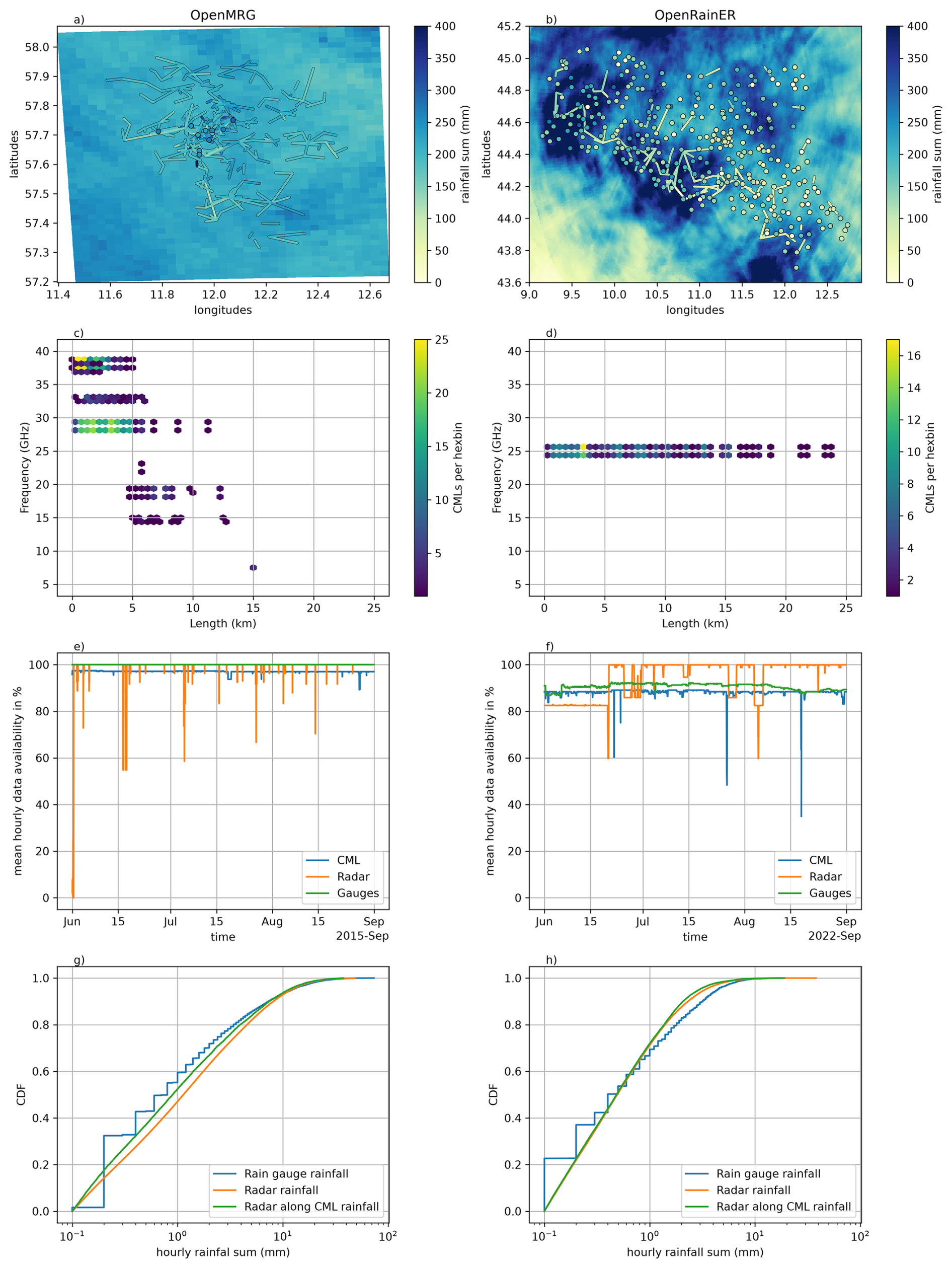
Figure 1 Maps and descriptive information on the OpenMRG (left column) OpenRainER (right column) dataset. (a) and (b) show the rainfall sum of the weather radar and the location of rain gauges and CMLs with their rainfall sum over the respective three month period. (c) and (d) show the distribution of CMLs over length and frequency. (e) and (f) show the mean hourly data availability. (g) and (h) show the cumulative distribution function over hourly rainfall sums.

The CML data was processed using a workflow following six steps:

1. Calculation of total signal loss. The total signal loss (TL) is calculated by subtracting RSL from the TSL.

2. Quality control. TL underwent the following quality control checks. We compared the channels for each link and removed the intervals in which the differences between attenuation levels were greater than 30 dB. In addition, CMLs were completely removed if they showed a strong diurnal cycle (5 h rolling standard deviation exceeding 2.0 dB for more than 10 % of the time) or excessively noisy signals (1 h rolling standard deviation exceeding 0.8 dB for more than 35 % of the time), following Graf et al. (2020), or showed no fluctuations (1 h rolling standard deviation below 0.8 dB for more than 99 % of the time).

3. Wet–dry classification. We used radar data to determine all wet time steps in CML data. For any radar time step along a CML path with more than 0.01 mm of rainfall per 15 min we marked that CML as wet. To account for temporal variability, a 5 min extension was added on each side of these wet periods.

4. Baseline estimation. The baseline was estimated using the mean of the 5 min TL before any wet period.

5. Wet antenna attenuation (WAA). WAA was estimated using the KR-alt model from Pastorek et al. (2022), with A_max=6, ζ=0.7 and d=0.15 and was subtracted from the TL.

6. k–R relation. The specific attenuation k (dB km⁻¹) caused by rainfall was converted to path-averaged rainfall intensity R (mm h⁻¹) using the empirical power-law relation k=aR^b, with frequency- and polarization-dependent coefficients a and b defined in ITU (2005).

All processing steps were already used in several other CML studies in Europe and Africa, some using identical parameters, some combined with other methods for individual steps (e.g. Blettner et al., 2022; Djibo et al., 2023; Graf et al., 2020; Øydvin et al., 2024; Van Weverberg et al., 2026). For other datasets and locations, the steps and parameters used here are a good starting point. Quality control should be adjusted for example if many long, low frequency CMLs are used as done by Blettner et al. (2025). Radar as wet–dry indicator needs of course radar data, otherwise, there are several methods using just TL. The WAA parameters have proven robust in several of the above mentioned studies and the ITU-R coefficients (a, b) are globally standardized based on frequency, polarization, and path elevation, making them directly transferable across study sites without requiring local calibration (ITU, 2005). All processing steps were implemented using pycomlink (Chwala et al., 2025).

3 Merging methods

To improve radar rainfall maps using CML observations, various merging methods have been implemented. These methods rely on paired radar (R(v)) and CML (R_CML(v)) rainfall estimates [mm h⁻¹] at location v. The radar rainfall R(v) is defined as the path-averaged radar rainfall along the CML, computed using the intersection weights between the CML path and the radar grid. This definition is the same for all merging methods. All methods use a local interpolation approach with a neighborhood of 70 radar–CML pairs, identified based on the distance between the target grid cell and the CML midpoints.

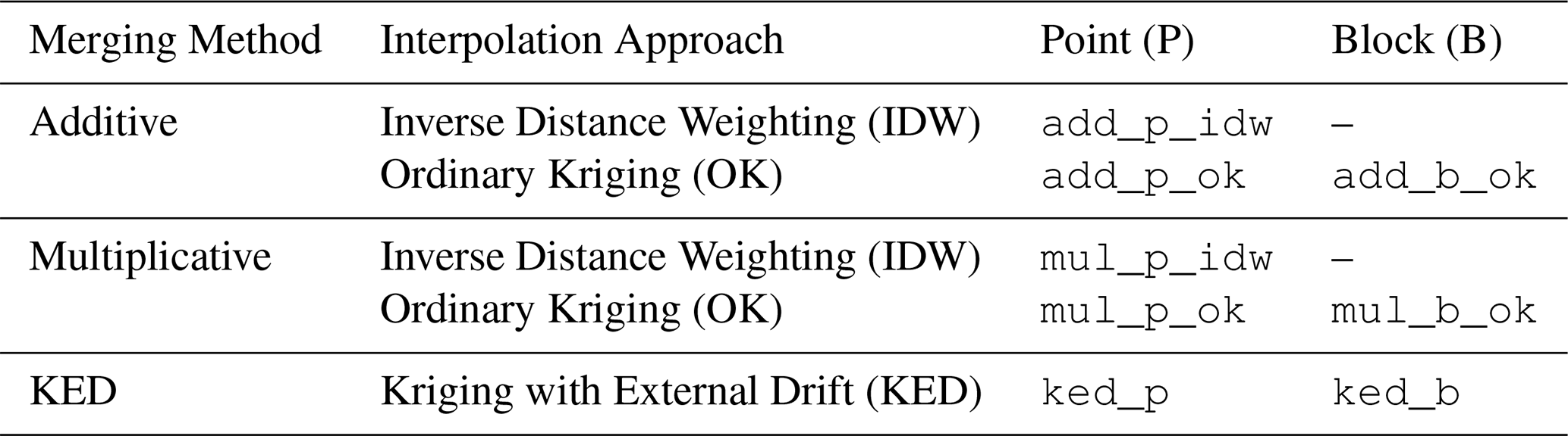
The merging process is applied independently for each time step, with both radar and CML data aggregated to an hourly resolution. Following the approach of previous studies (Jewell and Gaussiat, 2015; Goudenhoofdt and Delobbe, 2009; Velasco-Forero et al., 2009), the rainfall data is used in their original form rather than transforming them into Gaussian distribution. Table 1 shows an overview of the various merging methods used in the study.

3.1 Additive and multiplicative merging

Additive and multiplicative merging are methods for combining radar (R(v)) and CML (R_CML(v)) rainfall estimates. These methods represent two distinct physical hypotheses regarding radar error structures. Additive merging assumes that radar errors act as spatially varying offsets independent of rainfall intensity (e.g., range degradation, electronic drift, or partial beam blockage). Multiplicative merging, by contrast, assumes that radar errors scale proportionally with rainfall intensity (e.g., Z–R parameter mismatch, calibration offsets, or rain attenuation). The observed adjustment values at CML locations are denoted as D(v) for additive and F(v) for multiplicative merging, where:

• For additive merging: $D\left(v\right)=R_{\mathrm{CML}}\left(v\right)-R\left(v\right)$ (difference field),

• For multiplicative merging: $F\left(v\right)=\ln \left(\left(R_{\mathrm{CML}}\right(v)+\mathit{ϵ})/\left(R\right(v)+\mathit{ϵ})\right)$ (ratio field).

The small constant ϵ (e.g. 0.01) is added to the ratio to avoid issues with zero radar observations.

Range checks are applied to ensure reliable interpolation by excluding radar–CML pairs with large deviations. Unless otherwise stated, the following checks are used as the default:

• For Additive merging: $\left|R_{\mathrm{CML}}\right(v)-R(v\left)\right|\le \mathrm{10}\mathrm{mm}{\mathrm{h}}^{-\mathrm{1}}$,

• For Multiplicative merging: $\mathrm{0.1}\le R_{\mathrm{CML}}\left(v\right)/R\left(v\right)\le \mathrm{15}$ (dimensionless; thresholds are asymmetric by convention).

In additive merging, the interpolated field $\widehat{D}\left(v\right)$ is added back to the radar rainfall to produce the merged rainfall field:

$$\begin{array}{}\text{(1)}& R_{\mathrm{merged}}\left(v\right)=R\left(v\right)+\widehat{D}\left(v\right).\end{array}$$

In multiplicative merging, the interpolated field $\widehat{F}\left(v\right)$ is applied as a multiplicative factor to the radar rainfall:

$$\begin{array}{}\text{(2)}& R_{\mathrm{merged}}\left(v\right)=\left(R\left(v\right)+\mathit{ϵ}\right)\cdot \exp \left(\widehat{F}\right(v\left)\right)-\mathit{ϵ}.\end{array}$$

Finally, merged rainfall estimates exceeding 150 mm h⁻¹ are capped to that value to prevent physically unrealistic output from propagating into the merged fields.

3.2 Interpolation techniques

In both additive and multiplicative merging, the field Z(v) (either D(v) or F(v)) is interpolated to produce an estimate $\widehat{Z}\left(v\right)$ at unobserved locations, using one of the following techniques:

Inverse Distance Weighting (IDW). IDW estimates $\widehat{Z}\left(u_{\mathrm{0}}\right)$ at an unmeasured location v₀ as a weighted average of nearby observations Z(v_i):

$$\begin{array}{}\text{(3)}& \widehat{Z}\left(v_{\mathrm{0}}\right)={\displaystyle \frac{{\sum }_{i=\mathrm{1}}^N{w}_{\mathrm{i}}Z\left(v_i\right)}{{\sum }_{i=\mathrm{1}}^N{w}_{\mathrm{i}}}},w_{\mathrm{i}}={\displaystyle \frac{\mathrm{1}}{|v_i-v_{\mathrm{0}}{|}^{\mathit{\beta }}}},\end{array}$$

where w_i are the weights based on the inverse distance $|v_i-v_{\mathrm{0}}|$ between the observation location v_i and the target location v₀, and β controls how strongly the weights decay with distance. In this study we set β equal to 2. IDW is computationally efficient and easy to implement, but it does not account for spatial correlations.

Ordinary Kriging (OK), OK estimates $\widehat{Z}\left(v_{\mathrm{0}}\right)$ at a target location v₀ as a weighted sum of nearby observations Z(v_i):

$$\begin{array}{}\text{(4)}& \widehat{Z}\left(v_{\mathrm{0}}\right)=\sum _{i=\mathrm{1}}^N{\mathit{\lambda }}_{i}Z\left(v_i\right),\end{array}$$

The weights λ_i are determined by solving a constrained minimization problem that seeks the best linear unbiased estimator (BLUE) of Z(v₀). Specifically, the estimation variance

$$\begin{array}{}\text{(5)}& {\mathit{\sigma }}^{\mathrm{2}}=E\left[{\left(Z\left(v_{\mathrm{0}}\right)-\widehat{Z}\left(v_{\mathrm{0}}\right)\right)}^{\mathrm{2}}\right]\end{array}$$

is minimized subject to the unbiasedness constraint ${\sum }_{i=\mathrm{1}}^N{\mathit{\lambda }}_i=\mathrm{1}$. This yields the Kriging system of equations:

$$\begin{array}{}\text{(6)}& \sum _{j=\mathrm{1}}^N{\mathit{\lambda }}_{j}C\left(d_{ij}\right)+\mathit{\mu }=C\left(d_{i\mathrm{0}}\right),\sum _{i=\mathrm{1}}^N{\mathit{\lambda }}_i=\mathrm{1}.\end{array}$$

Here, C(d_ij) is the covariance between locations v_i and v_j, C(d_i0) is the covariance between v_i and the target location v₀, and μ is the Lagrange multiplier ensuring that the weights sum to 1.

3.3 Kriging with External Drift (KED)

KED extends OK by incorporating radar rainfall R(v) as an external spatial drift, assuming ground-level rainfall shares a domain-wide linear spatial relationship with radar intensity ($\mathit{\mu }\left(v\right)=a+b\cdot R\left(v\right)$). Physically, this unifies both the additive offset (a) and multiplicative scaling (b) error hypotheses into a single model, allowing baseline shifts and intensity-dependent adjustments to be estimated simultaneously.

KED builds on the OK system of equations (Eq. 6) with the addition of the drift constraint:

$$\begin{array}{}\text{(7)}& \sum _{i=\mathrm{1}}^N{\mathit{\lambda }}_{i}R\left(v_i\right)=R\left(v_{\mathrm{0}}\right),\end{array}$$

where R(v_i) is the radar rainfall at observation location v_i, R(v₀) is the radar rainfall at the target location v₀, and λ_i are the kriging weights obtained by solving the augmented system (Sideris et al., 2014; Jewell and Gaussiat, 2015).

3.4 Block Kriging

The methods described earlier assume point-based observations, which may not fully represent the spatial extent of line-averaged data such as CMLs. In this context, a block refers to the path of a CML link, a line segment over which the rainfall measurement is spatially averaged. To account for this, the kriging system is adapted to treat each CML as a block observation rather than a point. Block kriging minimizes the estimation variance of the block mean under the constraint of unbiasedness. Following the formulation in Journel and Huijbregts (1978, p. 306), the kriging system becomes:

$$\begin{array}{}\text{(8)}& \sum _{j=\mathrm{1}}^N{\mathit{\lambda }}_j{C}_{\mathrm{b}}(v_i,v_j)+\mathit{\mu }=C_{\mathrm{b}}(v_i,v_{\mathrm{0}}),\sum _{j=\mathrm{1}}^N{\mathit{\lambda }}_j=\mathrm{1},\end{array}$$

where C_b(v_i,v_j) denotes the covariance between block-averaged values. To correct for the smoothing effect of spatial averaging, this covariance is computed from the underlying point covariance C(h) as:

$$\begin{array}{}\text{(9)}& \begin{array}{rl}{C}_{\mathrm{b}}(v_i,v_j)& =C_{\mathrm{b}}\left(\mathrm{0}\right)+\stackrel{\mathrm{‾}}{C}(v_i,v_j)\\ & -{\displaystyle \frac{\mathrm{1}}{\mathrm{2}}}\left[\stackrel{\mathrm{‾}}{C}(v_i,v_i)+\stackrel{\mathrm{‾}}{C}(v_j,v_j)\right],\end{array}\end{array}$$

Here, $\stackrel{\mathrm{‾}}{C}(v_i,v_j)$ denotes the average point covariance between blocks v_i and v_j, while $\stackrel{\mathrm{‾}}{C}(v_i,v_i)$ and $\stackrel{\mathrm{‾}}{C}(v_j,v_j)$ represent the average point covariance within each block (see Appendix A for explicit definitions). The term C_b(0) corresponds to the sill of the block-averaged process.

A more detailed justification for Eq. (9) is given in Appendix A. Graf et al. (2021) and Goovaerts (2008) derive similar covariance expressions. For all kriging-based merging methods, the spatial structure of the data must be characterized by a theoretical variogram. While Goovaerts (2008) developed a deconvolution method for estimating the point variogram from block averaged data, Graf et al. (2021) used rain gauges to estimate the point variogram. In the next section, we describe a data-driven and a fixed approach for determining these parameters.

Table 1 Overview of merging methods and interpolation approaches.

3.5 Variogram estimation

To address the uncertainty in variogram selection, we implement two distinct strategies for determining the parameters of a spherical variogram model (Haberlandt, 2007): a data-driven strategy and a fixed strategy.

First, we estimate variogram parameters from the data. Building on Haberlandt (2007), who showed that event-averaged variograms result in minimal performance loss compared to fine temporal fitting, we adapt an similar event-pooling approach. Time steps are grouped into rainfall events: a time step is included in an event if the radar exceeds 0.01 mm h⁻¹ at any CML location, or is within 6 h of a time step that does. For each event, empirical semivariances are calculated from the respective target variables (i.e., radar–CML differences for additive merging and KED (Haberlandt, 2007), or ratios for multiplicative merging) exclusively at locations where radar rainfall exceeds zero. Pairwise semivariances are derived using Euclidean distances between CML midpoints and grouped into 1 km distance bins. A minimum of 100 observation pairs is required per event. If an event contains fewer than 100 pairs, pairs from neighbouring events are dynamically included in the pooling.

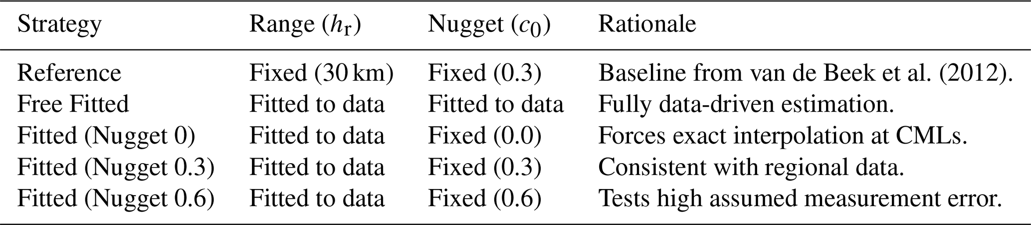
To reduce the number of parameters during optimization, the empirical variogram is standardized. Each bin's semivariance is divided by the average semivariance of all bins located between the 5th and 95th percentiles. This division removes the physical units and fixes the total sill to c=1, rendering the fitted parameters dimensionless, without affecting the resulting Kriging weights. Next, depending on the chosen strategy (Table 2), the range parameter h_r (and where applicable, the nugget c₀) is fitted by minimizing the sum of squares between the theoretical model and the standardized bins. To obtain a stable estimate that is representative for a longer period, the episode parameters are averaged over 14 d windows and applied to all time steps within that window.

Second, we use a fixed variogram. van de Beek et al. (2012) show that variogram parameters for 1 h Dutch summer rainfall have a range of approximately 30 km, though they also demonstrate that parameters vary substantially in time with rainfall characteristics. Since both datasets cover summer rainfall, we adopt the summer range as the fixed value h_r=30 km. Retaining this fixed value provides a benchmark against which data-estimated variograms are evaluated. The sill is set to c=1, and the dimensionless nugget c₀=0.3 is chosen to be broadly consistent with our data estimates.

To systematically evaluate the impact of these parameter choices on merging performance, we expanded these two strategies into a five-case sensitivity analysis (Table 2). The results of these configurations, detailed further in Sect. 4.3, isolate the effects of dynamic fitting versus fixed climatological parameters, as well as varying assumptions of measurement error. Based on the results of this sensitivity analysis, the reference strategy delivered comparable performance to the data-driven strategy while significantly reducing computational complexity and the risk of overfitting. Consequently, the fixed strategy was adopted as the standard configuration for all other merging throughout the remainder of this study.

van de Beek et al. (2012)

Table 2 Summary of variogram estimation strategies evaluated in the sensitivity analysis (Sect. 4.3).

3.6 Evaluation and metrics

Each of the eight merging methods (Table 1) produces an adjusted rainfall field based on CML data at an hourly resolution. These adjusted fields, along with the original radar rainfall field, are evaluated by extracting rainfall values at each rain gauge location $R_{g_i}$ from the nearest pixel in the rainfall field $R_{f_i}$, and computing metrics using poligrain (Chwala et al., 2024).

The root mean squared error (RMSE) evaluates the average magnitude of errors between observed ($R_{g_i}$) and estimated ($R_{f_i}$) rainfall, with larger errors penalized more heavily due to squaring:

$$\begin{array}{}\text{(10)}& \text{RMSE}=\sqrt{{\displaystyle \frac{\mathrm{1}}{N}}\sum _{i=\mathrm{1}}^N(R_{g_i}-R_{f_i}{)}^{\mathrm{2}}}\end{array}$$

The mean absolute error (MAE) provides the average magnitude of errors, treating all differences equally without emphasizing larger errors:

$$\begin{array}{}\text{(11)}& \text{MAE}={\displaystyle \frac{\mathrm{1}}{N}}\sum _{i=\mathrm{1}}^N|R_{g_i}-R_{f_i}|\end{array}$$

The percent bias (BIAS) quantifies the average bias as a percentage of the total observed rainfall, indicating whether the rainfall field systematically over- or underestimates rainfall:

$$\begin{array}{}\text{(12)}& \text{BIAS}={\displaystyle \frac{{\sum }_{i=\mathrm{1}}^N(R_{g_i}-R_{f_i})}{{\sum }_{i=\mathrm{1}}^N{R}_{g_i}}}\times \mathrm{100}\end{array}$$

The Pearson correlation coefficient (PCC) measures the strength and direction of the linear relationship between observed and estimated rainfall. Values range from −1 (perfect negative correlation) to 1 (perfect positive correlation), with 0 indicating no correlation:

$$\begin{array}{}\text{(13)}& \text{PCC}={\displaystyle \frac{{\sum }_{i=\mathrm{1}}^N(R_{g_i}-\stackrel{\mathrm{‾}}{R_g})(R_{f_i}-\stackrel{\mathrm{‾}}{R_f})}{\sqrt{{\sum }_{i=\mathrm{1}}^N(R_{g_i}-\stackrel{\mathrm{‾}}{R_g}{)}^{\mathrm{2}}{\sum }_{i=\mathrm{1}}^N(R_{f_i}-\stackrel{\mathrm{‾}}{R_f}{)}^{\mathrm{2}}}}}\end{array}$$

3.7 Reproducibility

A significant contribution of this work is the development of mergeplg, an open-source Python package for interpolation and merging of ground-based and radar-derived rainfall data (Øydvin et al., 2026a). The package optimizes workflows by updating CML coordinates and reusing kriging matrices across time steps. Built within the OpenSense data ecosystem (Chwala et al., 2026), mergeplg supports data from CMLs, PWSs, and radar systems, provided they follow the standardized OpenSense data format (Fencl et al., 2024). The package also integrates with poligrain (Chwala et al., 2024), a Python library for geospatial operations and visualization, enabling efficient tasks such as spatial queries (e.g., finding points near lines), plotting georeferenced data and computing metrics. By releasing mergeplg as open source, we aim to promote transparency, reproducibility, and collaboration, fostering its use and adaptation within the broader scientific community.

4 Results

4.1 Two overview case studies

Figure 2 provides a case study of the application of different merging methods of two 24 km² patches of OpenMRG (27 August 2015, 10:00 UTC) and OpenRainER (18 August 2022, 10:00). In the OpenMRG case, the radar field underestimates rainfall compared to rain gauges, while all merging methods reduce this underestimation to varying degrees. When comparing the rainfall fields, KED produces smoother fields overall, while additive retains more variability, and multiplicative introduces the strongest variability and sharper features. These differences are also reflected in the difference fields, where additive methods show smoother corrections compared to multiplicative. The difference fields of KED, on the other hand, exhibits greater spatial variability.

In the case reported for OpenRainER, the lower density of the CMLs makes it difficult to capture precipitation variability; however, we can appreciate a reduction in radar overestimation compared to the reference rain gauges. Looking at the difference fields, we can observe stronger radial symmetry for the IDW based methods, while kriging provides smoother corrections.

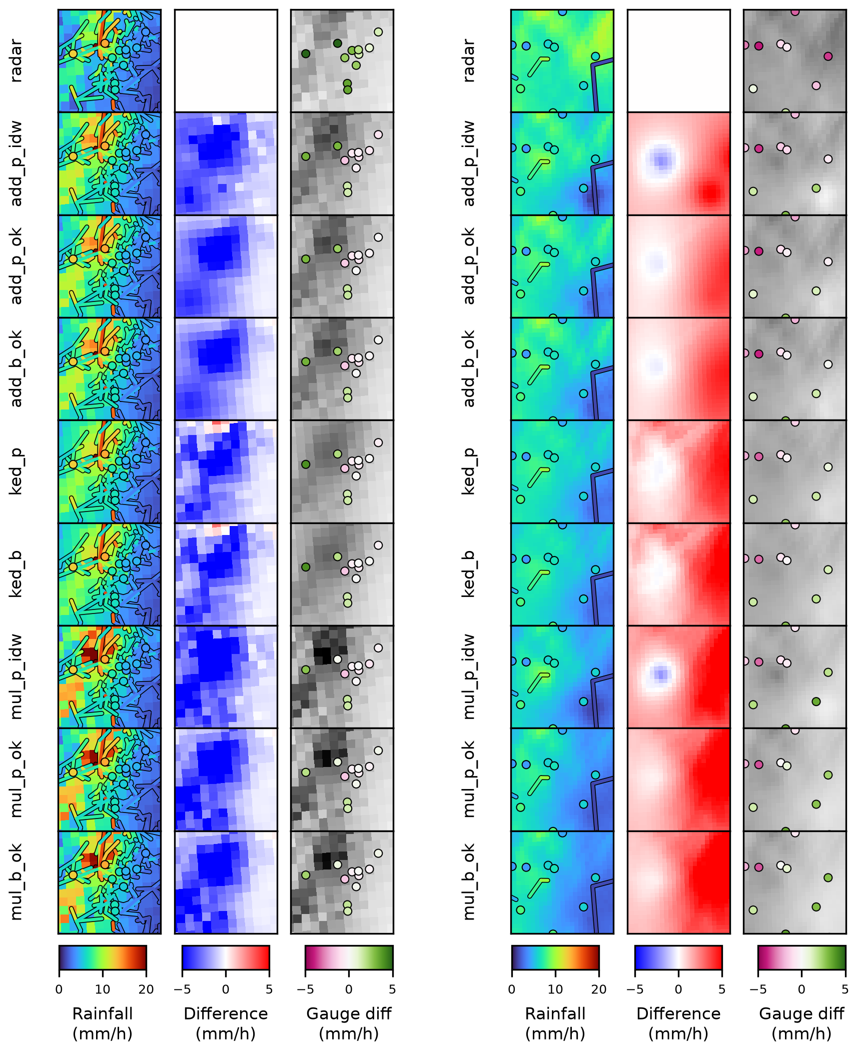
Figure 2 Case studies for both datasets. Left: OpenMRG, 27 August 2015, 10:00; Right: OpenRainER, 18 August 2022, 10:00. Each map shows an area of 24 km². The first column shows the 1 h rainfall maps, the second column shows the differences between the merged field and the original radar field, and the third column shows the differences between the fields and the rain gauges, with the rainfall field from each method shown as a gray-scale background for spatial context. Method acronyms (rows) are detailed in Table 1.

4.2 Variogram study

Using the per-event variogram fitting framework with free range and nugget parameters (Sect. 3.5), Fig. 3 shows the temporal evolution of event-fitted nugget and range values (with sill scaled to 1) for OpenMRG and OpenRainER. To evaluate spatial structure across inputs, we compare CML (blue) and gauge (orange) data across four field configurations: the target merging fields (radar–CML/gauge differences and ratios) and two diagnostic fields (CML/gauge alone and radar alone evaluated at CML midpoints or gauge locations).

In both datasets, CML data generally exhibit higher and more variable nugget and range values compared to gauge data. For radar-only fields, this variation is smaller, and the nugget is generally lower. Generally, the difference fields show larger variation than radar-only fields, followed by CML/gauge data; the ratio fields exhibit the largest variability in range and nugget estimates.

For OpenMRG, the range estimated directly from CML data is consistently larger than that from rain gauge data. This pattern also holds when using radar estimates at the CML midpoint or gauge location. This may be due to underestimation of range when rain gauges cover a small area (Western and Blöschl, 1999). In contrast, for OpenRainER, the range estimated from CML data is similar to the range estimated from rain gauge data and radar at the CML midpoint/gauge locations. This indicates that CML path-averaging does not substantially distort range estimates, and that 153 CMLs are sufficient to capture the spatial correlation scale, yielding results comparable to those from the 280 rain gauges.

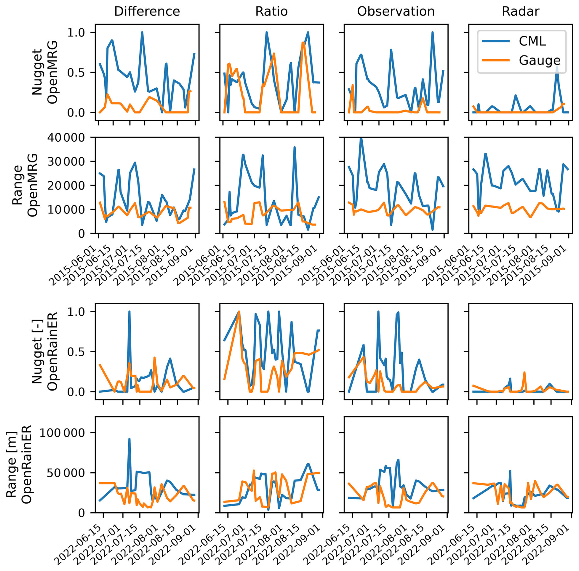
Figure 3 Variogram parameters (nugget and range; sill scaled to 1) are shown for OpenMRG (top two rows) and OpenRainER (bottom two rows). Columns represent: (1) difference between radar and CML/gauge; (2) ratio between radar and CML/gauge; (3) CML/gauge data alone; and (4) radar evaluated at CML midpoint (CML) or at gauge location (gauge). Colors distinguish CML (blue) and gauge (orange).

4.3 Impact of variogram parameters on interpolation

Figure 4 presents the RMSE values for the OpenMRG and OpenRainER datasets across the six kriging based merging variants (Table 1) and five variogram estimation strategies (Table 2).

In OpenMRG, a nugget of 0 produces moderately worse performance for all methods (RMSE increase of 0.07–0.15 mm), while on OpenRainER additive and KED methods are robust even to a zero nugget. Multiplicative methods show the strongest sensitivity to the nugget = 0 case on OpenRainER, where block kriging RMSE increases from approximately 2.90 to 4.78 mm. Among non-zero nugget strategies, the free nugget, fixed nugget at 0.3, and fixed nugget at 0.6 perform similarly across all methods, and the reference variogram parameters perform at least as well as any data-estimated strategy. Overall, the choice of variogram estimation strategy has little practical importance provided a non-zero nugget is used, with multiplicative block kriging on sparse networks being the most sensitive case. Consequently, because the reference fixed strategy performs comparably to data-driven fitting while reducing computational complexity, it was adopted as the standard configuration for all subsequent merging evaluations throughout the remainder of this study.

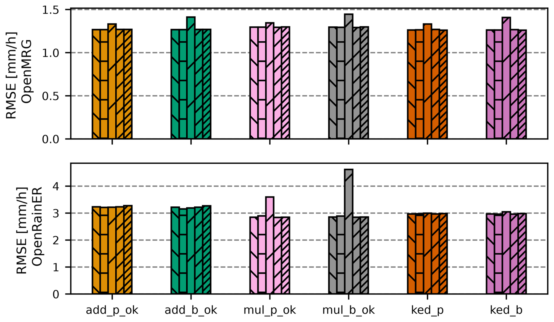
Figure 4 Root Mean Square Error (RMSE), for radar–CML six radar–CML merging methods across five variogram estimation strategies for the OpenMRG (top) and OpenRainER (bottom) datasets. Within each method group, the five bars represent variogram estimation strategies in strict left-to-right order: (1) constant range and nugget from van de Beek et al. (2012), (2) variogram fitted to data, (3) variogram fitted to data with nugget fixed at 0, (4) variogram fitted to data with nugget fixed at 0.3, and (5) variogram fitted to data with nugget fixed at 0.6 (Table 2). Method acronyms are detailed in Table 1.

4.4 Overall performance of adjustment methods

The performance of radar and merged radar–CML rainfall fields was evaluated at an hourly resolution using rain gauges as ground truth (Fig. 5). Overall, the OpenRainER dataset shows higher RMSE and MAE compared to the OpenMRG dataset, indicating greater variability and challenges in accurately estimating rainfall in this dataset.

Focusing on the OpenMRG dataset, all merging methods improve the radar field, with relatively similar performance across methods, although multiplicative methods exhibit slightly weaker performance overall. On average, MAE is reduced from 0.84 to 0.67 mm (20 %), RMSE is reduced from 1.44 to 1.28 mm (11 %), and PCC is increased from 0.55 to 0.69.

In contrast, the OpenRainER dataset exhibits more variation between merging methods. The radar has a RMSE of about 3.6 mm, which is reduced to 3.2 mm (11 %) for additive, 3.0 mm (17 %) for KED, and 2.9 mm (19 %) for multiplicative. In terms of MAE, the radar has a MAE of about 2.0 mm, which is reduced to 1.6 mm (21 %) for additive, 1.25 mm (38 %) for KED, and 1.18 mm (41 %) for kriging-based multiplicative (1.19 for IDW-based multiplicative).

In terms of PCC, the radar has a PCC of about 0.75, which is increased to 0.76 for additive and KED, but remains unchanged at 0.75 for kriging-based multiplicative (and drops to 0.73 for IDW-based multiplicative). In terms of BIAS, the radar has a BIAS of about 107 %, which is reduced to 35 % for additive, −6 % for KED and −1 % for multiplicative. Thus, multiplicative shows the smallest absolute BIAS and the best RMSE and MAE, while KED achieves a slightly higher PCC.

The effect of the block kriging correction is less pronounced, but compared to point kriging, it consistently reduces the relative BIAS, which can result in negative BIAS values becoming more negative.

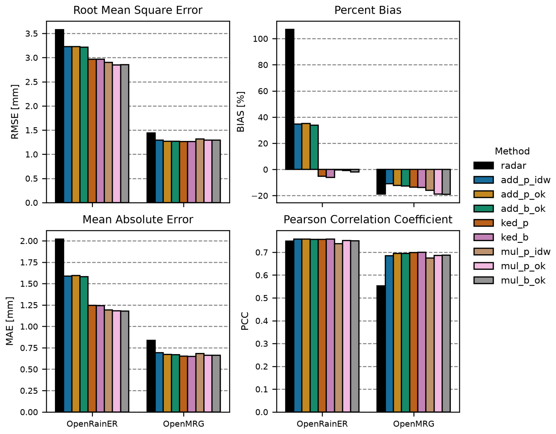
Figure 5 Root Mean Square Error (RMSE), Percent Bias (BIAS), Mean Absolute Error (MAE) and Pearson Correlation Coefficient (PCC) for all merging methods applied to the OpenRainER and OpenMRG datasets. Method acronyms are detailed in Table 1. All kriging based merging configurations use the reference fixed variogram strategy (Table 2).

4.5 Intensity-based analysis

To evaluate performance under varying rainfall intensities, an intensity-based analysis was performed (Fig. 6). Results are presented for four rainfall intensity bins, based on the rain gauge values: light rainfall $[\mathrm{0.2},\mathrm{2.5}]\mathrm{mm}{\mathrm{h}}^{-\mathrm{1}}$, moderate rainfall $[\mathrm{2.5},\mathrm{10}]\mathrm{mm}{\mathrm{h}}^{-\mathrm{1}}$, heavy rainfall $[\mathrm{10},\mathrm{50}]\mathrm{mm}{\mathrm{h}}^{-\mathrm{1}}$, and extreme rainfall ($>\mathrm{50}\mathrm{mm}{\mathrm{h}}^{-\mathrm{1}}$). Light rainfall constitutes 63.3 % of rainfall in OpenMRG (with 22.7 % with less than 0.2 mm h⁻¹) and 73.2 % in OpenRainER (with 1.6 % with less than 0.2 mm h⁻¹), therefore the light rainfall class reflects the results from overall performance analysis most. Generally, OpenRainER exhibits larger errors for light and moderate rainfall, but its radar outperforms the OpenMRG radar for heavy rainfall. Additionally, OpenRainER includes extreme rainfall events, which are absent in OpenMRG.

For OpenMRG, all merging methods consistently outperform the radar across all rainfall intensity bins, showing similar performance overall. The exception is heavy rainfall, where multiplicative methods perform slightly worse than additive and KED, with multiplicative IDW being the least good among them – though all methods still improve on the radar.

In contrast, OpenRainER shows greater variability between merging methods. For light and moderate rainfall, multiplicative and KED outperform additive, with multiplicative achieving the lowest RMSE overall. For heavy and extreme rainfall, radar and additive perform best, while KED and multiplicative show substantially higher RMSE. In terms of BIAS, OpenRainER shows a strong positive BIAS for low rainfall rates, which decreases with intensity, eventually becoming negative. OpenMRG exhibits a near-zero BIAS for low rainfall rates, which gradually decreases at higher intensities.

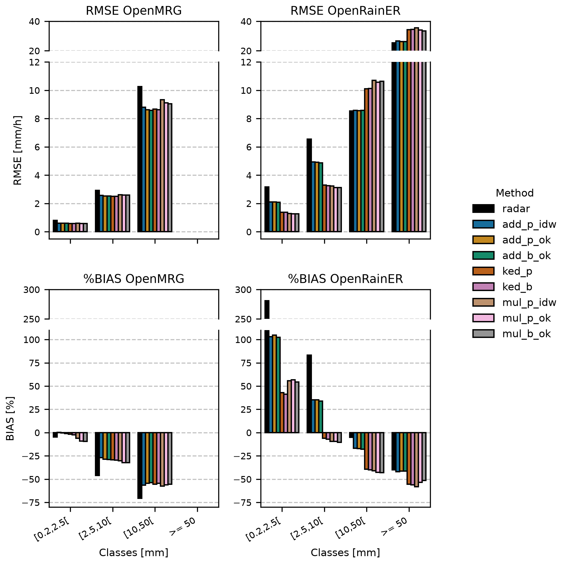
Figure 6 Root Mean Squared Error (RMSE) and Percent Bias (BIAS) for light rainfall $[\mathrm{0.2},\mathrm{2.5}]\mathrm{mm}{\mathrm{h}}^{-\mathrm{1}}$, moderate rainfall $[\mathrm{2.5},\mathrm{10}]\mathrm{mm}{\mathrm{h}}^{-\mathrm{1}}$, heavy rainfall $[\mathrm{10},\mathrm{50}]\mathrm{mm}{\mathrm{h}}^{-\mathrm{1}}$, and extreme rainfall ($>\mathrm{50}\mathrm{mm}{\mathrm{h}}^{-\mathrm{1}}$) for all merging methods applied to the OpenRainER and OpenMRG datasets. The intensity classes are based on rain gauges values. Method acronyms are detailed in Table 1. All kriging based merging configurations use the reference fixed variogram strategy (Table 2).

4.6 Distance-based analysis

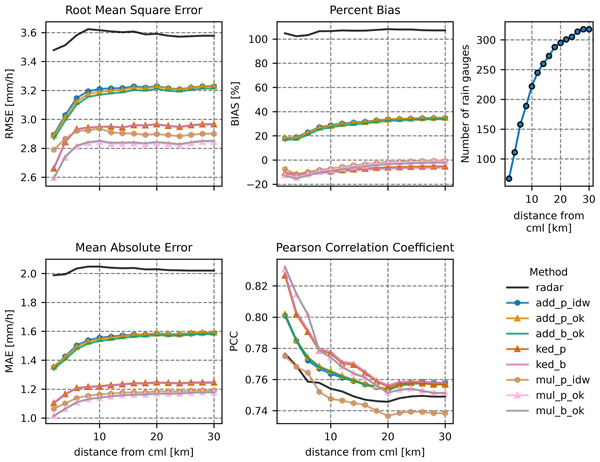
A distance-based analysis was performed on the OpenRainER dataset (Fig. 7). We grouped rain gauges into 2 km distance increments (e.g., 0–2, 0–4 km, etc.), with each group including all gauges within the specified range from a CML. The OpenMRG dataset was excluded here because its dense CML and rain gauge network caused all rain gauges to fall into the first distance bin, reducing the relevance of a distance-based analysis.

Generally, the distance-based analysis showed that all methods improve as the distance from CML decreases. In terms of RMSE and MAE, multiplicative kriging performed best at all distances, with RMSE approaching 2.6 mm h⁻¹ and MAE approaching 1.0 mm h⁻¹ at the closest distances. KED performed similarly, with RMSE approaching 2.7 mm and MAE approaching 1.1 mm. Additive methods performed worse, with RMSE approaching 2.9 mm and MAE approaching 1.4 mm. Notably, multiplicative IDW performs substantially worse than multiplicative kriging at close distances, approaching the performance of additive methods. In contrast, additive IDW performs similarly to additive kriging across all distances. Block kriging shows no clear improvement over point kriging at any distance.

In terms of BIAS, all merging methods reduce the radar BIAS of approximately 100 %. Additive methods have a positive BIAS that decreases as distance from CMLs decreases, approaching 20 % at the closest distances. Both KED and multiplicative methods have a negative BIAS that increases in magnitude as distance decreases, reaching about −10 % for KED and −13 % for multiplicative kriging at the closest distances. At far distances, multiplicative BIAS is closest to zero (−2 %), while KED is around −5 %.

In terms of PCC, additive, kriging based multiplicative, and KED outperform radar at all distances. Compared to additive, KED improves most rapidly with decreasing distance, achieving the highest PCC (0.83) near CMLs. Multiplicative IDW performs worse.

Interestingly, radar performance (RMSE and PCC) also improves slightly when rain gauges are near CMLs, potentially due to better radar coverage in those areas.

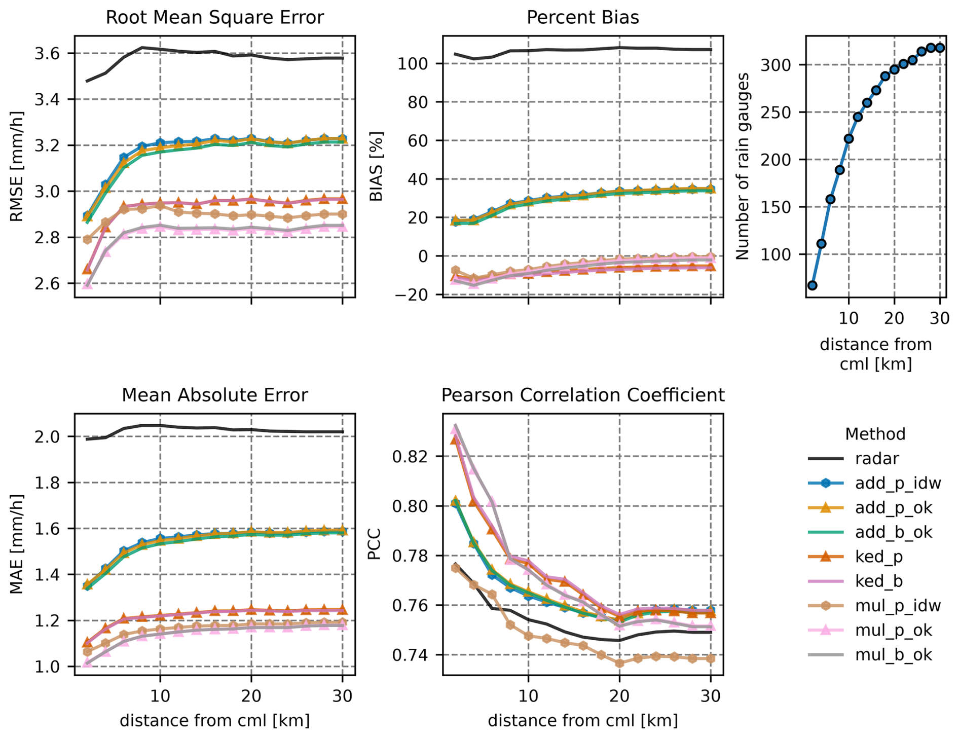
Figure 7 Root Mean Square Error (RMSE), Percent Bias (BIAS), Mean Absolute Error (MAE), and Pearson Correlation Coefficient (PCC) as functions of the maximum allowed distance between reference rain gauges and CMLs for all merging methods applied to the OpenRainER dataset. Rain gauges are grouped into 2 km distance increments, with each group including all gauges within the specified range from a CML. Method acronyms are detailed in Table 1. All kriging based merging configurations use the reference fixed variogram strategy (Table 2).

4.7 Sensitivity analysis of adjustment value range checks

A range check sensitivity analysis was performed to evaluate the impact of different range check thresholds on the merging methods (Fig. 8). Three range check configurations were tested: no check (no range check applied), standard, and strict. The thresholds for additive and KED methods were difference = 10 mm h⁻¹ (standard) and difference = 5 mm h⁻¹ (strict), while for Multiplicative methods they were ratio = [0.1, 15] (standard) and ratio = [0.2, 8] (strict). Under standard settings, the additive range check removed fewer than 2 % of valid CML-radar pairs in both datasets (0.0 % in OpenMRG, 1.4 % in OpenRainER). In contrast, the multiplicative range check removed 37.4 % of valid pairs in OpenMRG and 53.2 % in OpenRainER.

For the OpenMRG dataset, range checks had little impact on RMSE, and all combinations of merging methods and range checks improved the rainfall fields compared to radar alone. In the OpenRainER dataset, range checks play a more critical role: without them, merged fields can perform worse than radar alone, with KED RMSE exceeding the radar baseline of about 3.6 mm. Standard range checks are the preferred setting for additive and KED methods. For multiplicative methods, performance is similar between standard and strict settings, suggesting that any reasonable threshold is sufficient provided a check is applied.

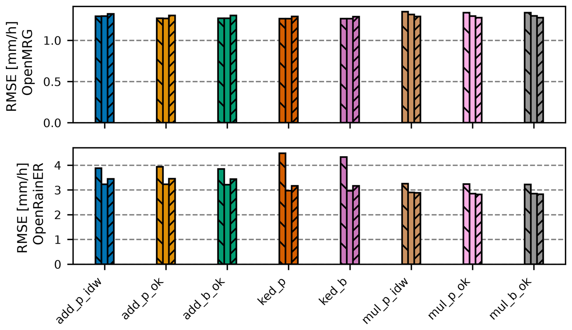
Figure 8 Root Mean Square Error (RMSE) for all merging methods under three range check configurations, shown in strict left-to-right order: (1) no check, (2) standard, and (3) strict, for the OpenMRG (top) and OpenRainER (bottom) datasets. Method acronyms are detailed in Table 1. All kriging based merging configurations use the reference fixed variogram strategy (Table 2).

4.8 Detailed case-studies

To better understand the strengths and limitations of the various merging methods, two case studies were performed (Figs. 9 and 10). The case studies span an area of approximately the same size, with the OpenRainER dataset covering longitude (9.6,10) and latitude (44.7,45), and the OpenMRG dataset covering longitude (11.8,12.2) and latitude (57.5,57.8).

The radar fields reveal differences in rainfall patterns between the two case studies. For OpenRainER, rainfall is more scattered, with several localized extremes, while for OpenMRG, rainfall is less scattered and concentrated along a single line. Additionally, the density of CMLs is much higher in the OpenMRG dataset, resulting in interpolated fields that are very similar across merging methods due to the dense observation network. In the OpenRainER dataset, differences between merging methods are more pronounced. At location (9.7,44.95), a CML observes approximately 40 mm, while the radar observes 10 mm. In the additive and KED merging methods, this CML observation is excluded by the range check (difference >10 mm). However, in the multiplicative merging methods, the ratio check (ratio = 4) does not flag the observation, and it is included. Since there are no nearby CMLs, this results in a large rainfall estimate in the merged field. While there are no nearby rain gauges to validate the observation, the resulting rainfall estimate appears overly high. At another location (9.75,44.8), the additive merging method excludes a CML observation due to the range check, while the multiplicative merging method retains it. A nearby rain gauge indicates that the CML measurement is likely correct, suggesting that this observation should have been included.

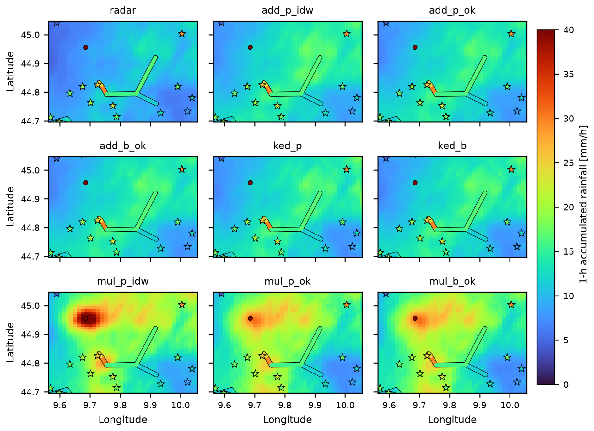
Figure 9 Spatial rainfall field from radar and merging methods for the OpenRainER dataset, with rain gauges (stars) and CMLs (lines) colored by rainfall amounts. Reference time: 18 August 2022, 10:00. Method acronyms are detailed in Table 1. All kriging based merging configurations use the reference fixed variogram strategy (Table 2).

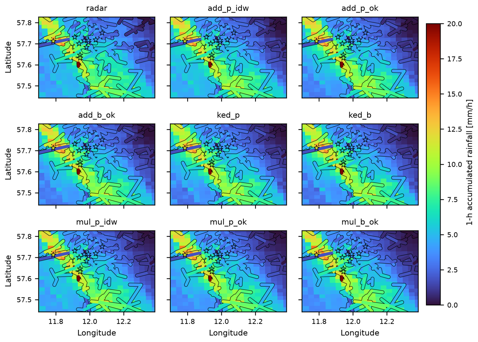
Figure 10 Spatial rainfall field from radar and merging methods for the OpenMRG dataset, with rain gauges (stars) and CMLs (lines) colored by rainfall amounts. Reference time: 25 August 2015, 08:00. Method acronyms are detailed in Table 1. All kriging based merging configurations use the reference fixed variogram strategy (Table 2).

5 Discussion

This section synthesizes our main findings on merging CML and radar data. We first examine how dataset characteristics and network density affect baseline merging accuracy, followed by an evaluation of additive, multiplicative, and KED paradigms. Next, we analyze the impact of geostatistical parameters, including variogram selection and point versus block kriging, before outlining practical takeaways and directions for future work.

5.1 Dataset characteristics and their influence on merging performance

The radar product in OpenMRG outperforms the OpenRainER for low and moderate rainfall. This could be due to the study area in OpenMRG having a relatively uniform terrain and moderate distance (78 km) to the closest weather radar (Andersson et al., 2022). Moreover, all rain gauges are located in the city center (Fig. 1), a localized area where the radar rainfall estimates appear to perform well. In contrast, OpenRainER covers a larger and more complex region with diverse terrain, contributing to higher errors. Despite this, OpenRainER’s radar outperforms OpenMRG's radar during heavy rainfall. This could be due to the capping applied to reflectivity in the dataset (Covi et al., 2026b), which helps prevent overestimation caused by hail but also limits the representation of extreme intensities.

The density of the CML network differs significantly between the two datasets, strongly influencing merging performance. OpenMRG benefits from a dense CML network (1 CML per 7.7 km², with even higher density near the majority of rain gauges in central Gothenburg), providing strong observational constraints that reduce variability in the merged fields and minimize differences between merging methods. For comparison, Nielsen et al. (2024) reported a similar observational density in Denmark (1 PWS per 2.1 km²). These densities are notably higher than in many other studies. For instance, Goudenhoofdt and Delobbe (2009) used a rain gauge network in Belgium with a density of 1 gauge per 135 km², Delrieu et al. (2014) used a dense network in the Cévennes-Vivarais region of France with 1 gauge per 128 km², and Jewell and Gaussiat (2015) used a sparser network in England and Wales with 1 gauge per 204 km². The density in OpenRainER (1 CML per 137 km²) is comparable to these earlier studies. However, unlike rain gauge networks, which are typically designed for even spatial coverage, CMLs are often concentrated along roads and urban areas. This uneven distribution can result in lower densities in some regions, posing challenges for merging methods.

The sparser observation network in OpenRainER increases reliance on radar, which can lead to greater uncertainty in the merged fields. Mismatches between radar and CML observations can arise due to spatial or temporal discrepancies, particularly in regions with complex terrain or areas where wind shifts rainfall patterns. These mismatches can lead to adjustments that do not reflect the actual rainfall distribution and sometimes cause large corrections and errors. For example, in the case study for OpenRainER (Fig. 9), we observed that sparse CML coverage in the north resulted in overcorrections, where a single CML observation drove adjustments over a large area. Conversely, in the south, strict range checks excluded valid CML observations.

5.2 Performance of merging methods

In OpenMRG, all merging methods improved the radar field, with additive and KED showing similar performance (e.g., 20 % MAE reduction). Multiplicative methods exhibited slightly higher errors and a negative bias, possibly because dense networks provide strong constraints that favor smoother methods like KED over the sharp gradients of multiplicative merging, or it could be due to potential biases in the CML rainfall retrieval algorithm (e.g. incorrect WAA parameters). In contrast, Nielsen et al. (2024) reported larger performance gaps between methods in a similarly dense network. A possible explanation is that their simpler adjustments, such as mean field bias (MFB) and inverse distance weighting interpolated bias (IDWB), lack the local neighborhood filtering inherent in their more advanced moving median bias (MMB) adjustment and in all our approaches. Our sensitivity analysis (Fig. B1) shows that performance is robust across various neighborhood sizes, even when using all observations. This indicates that spatial weighting combined with range checks provides sufficient inherent stability in dense networks, rendering neighborhood restriction largely unnecessary to protect against far-away outliers. While we did not implement MMB, our results suggest that future work should isolate whether robust median-based filtering offers benefits beyond spatial weighting and range checks alone.

In contrast, OpenRainER exhibits more variation between merging methods. The improvements observed in OpenRainER are consistent with findings from other studies, with similar network densities. For example, Goudenhoofdt and Delobbe (2009) found that KED and kriging with radar-based error correction reduced radar MAE by about 40 % for daily rainfall in Belgium. Similarly, Jewell and Gaussiat (2015) reported significant reductions in RMSE and MAE for hourly rainfall at different rainfall intensities for KED in England and Wales, with improvements of up to 30 %–40 % in MAE and 25 %–40 % in RMSE. In OpenRainER, reductions in MAE were 21 % for additive, 41 % for multiplicative, and 38 % for KED, aligning well with these earlier findings. Overeem et al. (2024b) found that PWS reduced radar MAE by 20 % in a European wide study. However, the reductions in RMSE were more modest: 10 % for additive, 17 % for KED and 19 % for multiplicative. This could be due to the less evenly distributed CML network and the complex terrain, which amplify radar–CML mismatches and create greater uncertainty in merged fields. It could also be due to signal fluctuations causing CML rainfall outliers, or the path averaging effect of the CML dampening rainfall extremes.

Multiplicative merging achieves the best overall RMSE and MAE in OpenRainER, and the smallest absolute BIAS (−2 %). This indicates that radar errors in OpenRainER are largely intensity-dependent, aligning with the physical mechanisms outlined earlier, such as Z–R parameter mismatches. While both KED and multiplicative merging allow for intensity-dependent corrections, standard KED assumes a uniform scaling slope (b), whereas multiplicative merging inherently accommodates spatially changing ratios. Implementing KED with local search neighborhoods enables b to adjust regionally across the 70 nearest stations, narrowing this conceptual gap. However, fitting a single linear regression within each window still forces b into a regional compromise, whereas multiplicative kriging directly interpolates continuous ratio fields, offering a more flexible spatial correction that likely accounts for its superior performance.

Further, additive methods outperform multiplicative and KED during heavy and extreme rainfall (Fig. 6). This is likely because extreme events are often driven by localized rainfall regimes, such as convective storms, which feature sharp spatial intensity gradients. Under these conditions, additive merging provides a more robust local adjustment by boosting peak rates without altering the radar's spatial pattern or high correlation. Multiplicative merging, by contrast, risks creating nonphysical high-intensity artifacts near storm cores, because a fixed global variogram smooths ratio factors over too broad an area. Furthermore, multiplicative scaling is highly sensitive to isolated CML errors in sparse networks, as illustrated in the case study (Fig. 9), where a single unchecked CML produced a large overcorrection. KED's underperformance during extreme events could also be explained by its inherent tendency to produce smoother rainfall fields (as observed in Fig. 2). Fundamentally, KED assumes a linear relationship between CMLs and radar ($\mathit{\mu }\left(v\right)=a+b\cdot R\left(v\right)$). Because path-averaged CMLs inherently dampen localized extremes, this linear trend is fitted to a flattened response, restricting its ability to resolve sharp peaks. Additionally, because external drift was applied unconditionally in this study without prior statistical testing, enforcing the linear drift when radar explanatory power was weak likely forced the interpolation into an artificially smoothed or distorted state during severe storms.

In OpenMRG, the improvement in radar PCC after merging is substantial (from 0.55 to 0.70 with KED), aligning with earlier findings. For example, Delrieu et al. (2014) reported radar PCC values of 0.4–0.9 improving to 0.8–0.9 with KED for hourly rainfall in France. In contrast, OpenRainER shows only a modest PCC improvement (0.75 to 0.76), reflecting the already high correlation between radar and reference data. The MAE pattern is reversed: OpenMRG shows a smaller relative improvement while OpenRainER improves substantially, indicating that merging in OpenRainER primarily corrects magnitude errors rather than spatial pattern. These dataset-dependencies, driven by terrain, rainfall type, sensor distribution, and radar quality, make cross-study comparisons of merging scores challenging. Moreover, validation gauges themselves carry biases such as wind undercatch (Nešpor and Sevruk, 1999), further complicating evaluation.

5.3 Variogram estimation and its effect on merging performance

The variogram study (Fig. 3) reveals systematic differences between observation types and datasets. In OpenMRG, the spatial range estimated from CML observations is consistently larger than that from rain gauges. On one hand, this could be explained by CML path averaging inflating the apparent correlation length by smoothing fine scale variability (Eshel et al., 2022). However, the same pattern also holds when comparing point-scale radar evaluated at CML midpoints versus radar at gauge locations, indicating that path-averaging is not the primary driver. This points to a spatial extent effect rather than path-averaging. As Western and Blöschl (1999) show, the apparent correlation length is biased low when the sampling domain is small relative to the true correlation length. In OpenMRG, this effect is pronounced because rain gauges are confined to the city center while CMLs span the wider network. In contrast, CML- and gauge-estimated ranges are similar in OpenRainER, where both sensor networks cover comparable spatial extents. Taken together, these findings suggest that CML path-averaging does not exert a strong influence on spatial range estimates at the scales used in this study.

Despite the pronounced temporal variability in fitted variogram parameters (Fig. 3), merging performance remains remarkably stable across different parameter estimation strategies (Fig. 4). Theoretically, this stability could stem from two potential mechanisms related to variogram behavior. First, spatial interpolation over short distances between sensors is dictated by near origin behavior, raising the hypothesis that a stable initial slope, represented by the ratio of sill to range $(\mathrm{1}-c_{\mathrm{0}})/h_{\mathrm{r}}$, buffers parameter variations. However, dynamically fitted nuggets and ranges fluctuate strongly and independently over time (Fig. 3), causing this gradient to vary wildly across storm events. Moreover, adopting fixed parameters from the literature achieves almost identical merging performance compared to approaches where the parameters are estimated from data (Fig. 4), suggesting that performance stability does not depend on capturing variogram gradients unique to each storm. Second, parameter sensitivity would be reduced if spatial error fields exhibited systematically longer, smoother correlation ranges than raw rainfall. Yet, empirical variograms of residual and ratio fields show no such lengthening (Fig. 3), possibly because primary radar errors scale directly with rainfall intensity. Instead, the stability of merging performance stems primarily from the spatial weighting structure of the algorithms themselves, which inherently smooths local corrections even under imperfect variogram specifications while remaining tightly constrained by observational values at sensor locations.

While specific range values have a limited practical impact, the inclusion of a non-zero nugget is essential for maintaining this performance. A zero nugget forces exact interpolation at CML locations, which can lead to the amplification of local errors and artifacts – especially for multiplicative methods in sparse networks where local uncertainties are high. This is corroborated by Haberlandt (2007), who found that a simple linear variogram with zero nugget resulted in the largest errors (highest RMSE) among all tested models. Because spatial weighting is heavily influenced by short-to-moderate distances where linear and spherical models exhibit similar behavior, it is highly likely that the lack of a nugget, rather than the linear model itself, was a primary contributor to the high errors observed in that study. In contrast, their more effective models utilized spherical structures and standardized nuggets between 0.1 and 0.4. Our results confirm that while a reference variogram serves as a robust default, a non-zero nugget is critical for reliable geostatistical merging.

While this study selected a spherical variogram model and moving-window pooling a priori based on established rainfall merging literature (e.g., Haberlandt, 2007, and van de Beek et al., 2012), neither alternative model shapes (e.g., exponential or Gaussian) nor finer, timestep-specific variogram fitting were explicitly evaluated. However, our sensitivity analysis (Fig. 4) demonstrated that overall merging performance remained largely invariant across a broad range of variogram parameters, consistent with findings by Haberlandt (2007) that dynamic hourly fitting yields negligible overall gains compared to temporal pooling. Nevertheless, finer temporal or spatially dynamic fitting could still prove beneficial during sharp convective transitions – particularly for multiplicative merging, where large-scale, domain-pooled correlation ranges risk over-extending local ratio adjustments. Ultimately, while the isolated impacts of alternative functional forms and finer fitting scales remain formally untested here, these choices are expected to play secondary roles relative to the spatial weighting structure of the algorithms and the inclusion of an appropriate non-zero nugget.

5.4 Comparison of interpolation methods

For the merging methods (additive, multiplicative, and KED), different interpolation approaches were used. These approaches include IDW, point kriging, and block kriging (Table 1).

Theoretically, block kriging should outperform point kriging by accounting for the line-integral nature of CMLs. However, both methods yield nearly identical results in this study. In the sparse OpenRainER dataset, this parity is likely because the massive 107 % radar bias makes the path-mean magnitude the primary driver of performance, rendering geometry a secondary refinement. Conversely, in the dense OpenMRG network, the high density of observations in combination with a relatively high nugget value constrains the interpolated fields so effectively that the choice between point and block representations has little practical impact. Furthermore, the large correlation lengths (approximately 30 km) and high nugget values (approximately 0.3 mm h⁻¹) identified in the variogram study minimize the impact of line-averaging across both datasets, allowing a midpoint point-approximation to effectively represent the local rainfall state. Nevertheless, block kriging may offer a latent advantage through its uncertainty estimates near CML observations, which could be used to blend merged and radar-only fields (Lussana et al., 2025; Delrieu et al., 2014), though this was not demonstrated in the present study.

The advantages of kriging become more apparent in multiplicative merging. Here, IDW performed worst, while point and block kriging showed similar performance. Distance analysis reveals this gap is most pronounced near CMLs. Because multiplicative merging produces adjustment fields with sharper gradients, kriging's spatial weighting and nugget effect likely provide essential stability that IDW lacks.

Block kriging's lack of improvement upon ordinary kriging may stem from the fact that kriging estimates the conditional expectation. Consequently, point-scale variability remains elusive regardless of path-averaging corrections. Capturing more complex, intermittent, or anisotropic structures may require stochastic spatial reconstructions (Green et al., 2024; Leblois and Creutin, 2013; Blettner et al., 2022; Roksvåg et al., 2020) or non-linear covariate integration (Sideris et al., 2014; Ingebrigtsen et al., 2015).

5.5 What we learned from working with the data and further work

Adjusted fields performed best close to the CMLs, indicating that radar–CML bias varies spatially. This finding is consistent with earlier work (Goudenhoofdt and Delobbe, 2009), which showed that spatially varying adjustment methods outperform a single mean correction factor applied across the entire field. Such variability in radar bias can arise from differences in radar beam height, precipitation type, or terrain. Both radar and CMLs tend to overestimate precipitation in wet snow conditions, while dry snow is not detected by CMLs (Øydvin et al., 2025). In OpenRainER, the impact of wet snow is partly reduced by capping radar values. However, this cap complicates merging, as it introduces nonlinearity in the relationship between radar and ground observations. Further works should explore how external data, such as atmospheric models or terrain data (which are often incorporated into model data; Lussana et al., 2021) could be combined to make merging CML more robust.

Range checks are essential, particularly for OpenRainER. Without them, merged fields often perform worse than radar alone due to the presence of outliers. The reason OpenMRG is less sensitive to range checks could be the high density CML network in combination with a few rain gauges in the city center, where outlier data are quickly canceled. Another explanation could be that the rainfall intensities are lower in the OpenMRG dataset, causing fewer large outliers. The heightened sensitivity of the OpenRainER dataset also reflects its specific network configuration; operating within a narrow frequency band (24.6–25.6 GHz), link sensitivity varies significantly with length, complicating the application of uniform range checks. The coarser signal quantization in OpenRainER (1 dB) may also contribute to differences in data quality, which could also explain the grater sensitivity to range checks. The stringency of these checks also varies significantly by method: multiplicative range checks removed 37 % of observations in OpenMRG and 53 % in OpenRainER, whereas additive checks removed less than 2 %. This disparity could be driven by the inherent sensitivity of ratio-based checks to near-zero radar values, where even minor CML signals produce large ratios. Future efforts should investigate dynamic range checks capable of adapting to varying rainfall intensities and local network geometries.

The uncertainty of CML-derived rainfall estimates is driven by several processing steps, including wet–dry classification, baseline estimation, and WAA correction (Chwala and Kunstmann, 2019). In this study, identifying wet periods via radar simplifies the workflow, but errors in the timing of wet-period boundaries or the introduction of intermittent radar artifacts can lead to elevated baseline estimates and biased rainfall retrievals (Øydvin et al., 2024). Because these processing strategies are applied across the entire network, they can introduce systematic biases rather than just random local noise. These errors propagate directly into the merged rainfall field. Since geostatistical merging assumes that ground-based observations represent the truth, a network-wide bias in CML data will systematically shift the radar estimates toward that bias. Consequently, a merging method that provides a more correct bias correction may paradoxically yield a result that is more wrong than a less sensitive method; by more effectively forcing the radar to match a biased CML reference, the more effective method shifts the final estimate further from the actual rainfall. Geostatistical methods can incorporate measurement uncertainty and micro scale variability into the nugget effect, or even handle point specific error variances via Kriging for Uncertain Data (Cecinati et al., 2018). However, because these parameterizations assume zero mean random noise, they cannot inherently resolve or compensate for network wide systematic biases. While dense networks can average out random local artifacts, they remain vulnerable to these systemic processing errors, which can degrade performance regardless of observational density. This could explain the stronger BIAS observed in the OpenMRG dataset, as compared to OpenRainER. While the same dataset also show less good PCC, indicating that errors are not solely due to stronger BIAS, a poor WAA model could still cause distorted rainfall estimates. Further work is needed to evaluate how radar-based processing affects these systematic biases and to explore more robust methods for integrating CML data without propagating these inherent uncertainties.

While this study focused on neighborhood-based merging methods, many other combinations remain to be explored. Neighborhoods could be extended to include both short- and long-range components, as in Overeem et al. (2023), or alternative approaches such as the median-based adjustment proposed by Nielsen et al. (2024). Exploring these options would help clarify how different neighborhood definitions and filtering strategies influence merging performance across diverse datasets.

6 Conclusions

In this work, we developed mergeplg, an open-source Python package for merging radar and CML rainfall data, to assess the impact of diverse merging strategies across varying network densities. The package and accompanying notebooks are released to promote openness, reproducibility, and usability (Øydvin et al., 2026a; Covi et al., 2026a).

Our analysis demonstrates that merging radar and CML data consistently improves rainfall estimates, especially when the CML network is dense and close to rain gauges, but the degree of improvement depends on terrain, rainfall type, and radar quality. In OpenMRG, the improvement in PCC after merging is substantial (from 0.55 to 0.70), while the reduction in MAE is more modest (20 %). In contrast, OpenRainER’s sparser network saw only a slight increase in PCC (from 0.75 to 0.76) but a much larger reduction in MAE (up to 41 % for multiplicative merging), suggesting that while the overall rainfall pattern was already well captured by the radar, merging primarily served to correct magnitude errors and biases. Although MAE improvements align with rain gauge benchmark studies, RMSE gains were more modest (19 % for multiplicative merging), pointing to higher noise levels in CML observations relative to traditional gauges, a characteristic further reflected by the relatively large estimated nugget value (30 % of the sill).

Our results further highlight that merging effectiveness is strongly dependent on merging method and dataset. While all methods perform comparably in data-dense settings, additive methods are still more effective for capturing peak rainfall intensities. In data-sparse settings, multiplicative and KED achieves the lowest overall RMSE and MAE, while additive methods still better capture peak rainfall intensities. This indicates that, for low and medium rainfall intensities, radar errors for this particular dataset is more driven by scaling errors (e.g., Z–R parameter mismatch, calibration offsets, or rain attenuation), rather than spatial varying offsets (e.g., range degradation, electronic drift, or partial beam blockage). Furthermore, because CML and rain gauge observations carry their own measurement errors, superior merging algorithms may produce suboptimal results when supplied with inaccurate input data.

Regarding geostatistical parameters, all methods proved robust to variogram choice provided a non-zero nugget was used. While kriging approaches outperformed IDW in multiplicative merging, block kriging showed no consistent advantage over point kriging in either sparse or dense network settings. This suggests that path-averaging corrections alone do not overcome the smoothing inherent in conditional expectation estimates. Finally, we conclude that robust range checks are essential for stability, particularly for multiplicative methods where ratio-based checks are sensitive to near-zero radar values.

Overall, this work demonstrates the clear value of combining radar and CML data for improved rainfall estimation and offers guidance on selecting merging methods for both dense and sparse networks, supporting more accurate hydrometeorological applications.

Appendix A: Block Covariance from Point-Support Structure

We refer to spatially averaged observations, such as CML path-integrated measurements, as block data. Although our focus is on path-averaged observations, the methodology applies to blocks of arbitrary shape and orientation. These block averages are assumed to arise from an underlying second-order stationary spatial process Z(x). Under second-order stationarity, the semi-variogram γ and covariance function C are related by:

$$\begin{array}{}\text{(A1)}& \mathit{\gamma }(h\mid \mathit{\theta })=C(\mathrm{0}\mid \mathit{\theta })-C(h\mid \mathit{\theta }),\end{array}$$

where C(h∣θ) is the covariance function and C(0∣θ) is the sill, equal to the sum of spatial variance and the variance at h=0. The parameter vector θ defines the covariance model. Assuming the observation errors are not correlated, the diagonal entries of the covariance matrix can be modified by adding the estimated error for each observation (Cecinati et al., 2018), and the covariance matrix becomes:

$$\begin{array}{}\text{(A2)}& {\mathbf{C}}_{ij}=\left\{\begin{array}{ll}c+c_{\mathrm{i}},& \text{if }i=j\\ C(v_i-v_j)=c-\mathit{\gamma }& \text{if }i\ne j\end{array}\right.\end{array}$$

where c is the spatial variance of the point process and c_i is the individual uncertainty of each observation v_i and v_j.

Next, as shown in Journel and Huijbregts (1978, p. 54), the expected squared difference between two block averages $Z_{v_i}$ and $Z_{v_j}$ can be expressed in terms of the underlying point-support covariance function:

$$\begin{array}{}\text{(A3)}& \mathbb{E}\left[\right(Z_{v_i}-Z_{v_j}{)}^{\mathrm{2}}]=\stackrel{\mathrm{‾}}{C}(v_j,v_j)+\stackrel{\mathrm{‾}}{C}(v_i,v_i)-\mathrm{2}\stackrel{\mathrm{‾}}{C}(v_i,v_j),\end{array}$$

where $\stackrel{\mathrm{‾}}{C}(v_i,v_i)$ and $\stackrel{\mathrm{‾}}{C}(v_j,v_j)$ are the average point covariances within blocks v_i and v_j, and $\stackrel{\mathrm{‾}}{C}(v_i,v_j)$ is the average point covariance between them. Furthermore, the block-averaged process inherits second-order stationarity, allowing us to write a semi-variogram identity for block data:

$$\begin{array}{}\text{(A4)}& \mathbb{E}\left[\right(Z_{v_i}-Z_{v_j}{)}^{\mathrm{2}}]=\mathrm{2}\left[C_{\mathrm{b}}\left(\mathrm{0}\right)-C_{\mathrm{b}}(v_i,v_j)\right],\end{array}$$

C_b(v_i,v_j) is the covariance function of the block averaged data and C_b(0) is the sill, equal to the variance of the block averaged data. Combining Eqs. (A3) and (A4), we obtain:

$$\begin{array}{}\text{(A5)}& \mathrm{2}\left[C_{\mathrm{b}}\left(\mathrm{0}\right)-C_{\mathrm{b}}(v_i,v_j)\right]=\stackrel{\mathrm{‾}}{C}(v_i,v_i)+\stackrel{\mathrm{‾}}{C}(v_j,v_j)-\mathrm{2}\stackrel{\mathrm{‾}}{C}(v_i,v_j),\end{array}$$

which leads to the block covariance expression:

$$\begin{array}{}\text{(A6)}& \begin{array}{rl}{C}_{\mathrm{b}}(v_i,v_j)& =C_{\mathrm{b}}\left(\mathrm{0}\right)+\stackrel{\mathrm{‾}}{C}(v_i,v_j)\\ & -{\displaystyle \frac{\mathrm{1}}{\mathrm{2}}}\left[\stackrel{\mathrm{‾}}{C}(v_i,v_i)+\stackrel{\mathrm{‾}}{C}(v_j,v_j)\right].\end{array}\end{array}$$

A common approach is to work with the semi-variogram when evaluating the correlation between observations (Murphy et al., 2025). We expand this approach to block kriging. Inserting Eq. (A6) into the ordinary kriging system (Eq. 8) we get

$$\begin{array}{}\text{(A7)}& \begin{array}{rl}\sum _{j=\mathrm{1}}^N{\mathit{\lambda }}_j\mathit{\left\{}{C}_{\mathrm{b}}\right(\mathrm{0})& +\stackrel{\mathrm{‾}}{C}(v_i,v_j)-{\displaystyle \frac{\mathrm{1}}{\mathrm{2}}}\left[\stackrel{\mathrm{‾}}{C}\right(v_i,v_i)+\stackrel{\mathrm{‾}}{C}(v_j,v_j\left)\right]\mathit{\}}\\ & +\mathit{\mu }=C_{\mathrm{b}}\left(\mathrm{0}\right)+\stackrel{\mathrm{‾}}{C}(v_i,p)\\ & -{\displaystyle \frac{\mathrm{1}}{\mathrm{2}}}\left[\stackrel{\mathrm{‾}}{C}\right(v_i,v_i)+\stackrel{\mathrm{‾}}{C}(p,p\left)\right]\end{array}\end{array}$$

Where v_i denotes block i and v_j denotes another block j. Following Eq. (A4) averaged covariance can be expressed in terms of averaged semi-variance, the sill cancels between the block-block and within-block covariances and we get

$$\begin{array}{}\text{(A8)}& \begin{array}{rl}\sum _{j=\mathrm{1}}^N{\mathit{\lambda }}_j\mathit{\left\{}{C}_{\mathrm{b}}\right(\mathrm{0})& -\stackrel{\mathrm{‾}}{\mathit{\gamma }}(v_i,v_j)+{\displaystyle \frac{\mathrm{1}}{\mathrm{2}}}\left[\stackrel{\mathrm{‾}}{\mathit{\gamma }}\right(v_i,v_i)+\stackrel{\mathrm{‾}}{\mathit{\gamma }}(v_j,v_j\left)\right]\mathit{\}}\\ & +\mathit{\mu }=C_{\mathrm{b}}\left(\mathrm{0}\right)-\stackrel{\mathrm{‾}}{\mathit{\gamma }}(v_i,p)\\ & +{\displaystyle \frac{\mathrm{1}}{\mathrm{2}}}\left[\stackrel{\mathrm{‾}}{\mathit{\gamma }}\right(v_i,v_i)+\stackrel{\mathrm{‾}}{\mathit{\gamma }}(p,p\left)\right],\end{array}\end{array}$$

where p is the point we want to predict to. Following Eq. (A2), C_b(0) on the r.h.s is not evaluated at h=0, and is thus just the spatial variance of the data c added to all entries in the vector. C_b(0) on the l.h.s contributes c to all cross-terms of the matrix and c+c_i to the diagonal. Since $c{\sum }_{j=\mathrm{1}}^N{\mathit{\lambda }}_j=c$ under ${\sum }_{j=\mathrm{1}}^N{\mathit{\lambda }}_j=\mathrm{1}$, the constant c cancels on both sides, and we get the following system of equations:

$$\begin{array}{}\text{(A9)}& \begin{array}{rl}& \left[\begin{array}{rl}& \left[\begin{array}{ccccc}{c}_{\mathrm{1}}& \mathrm{0}& \mathrm{\dots }& \mathrm{0}& \mathrm{0}\\ \mathrm{0}& c_{\mathrm{2}}& \mathrm{\dots }& \mathrm{0}& \mathrm{0}\\ \mathrm{⋮}& \mathrm{⋮}& \mathrm{\ddots }& \mathrm{⋮}& \mathrm{⋮}\\ \mathrm{0}& \mathrm{0}& \mathrm{\dots }& c_n& \mathrm{0}\\ \mathrm{0}& \mathrm{0}& \mathrm{\dots }& \mathrm{0}& \mathrm{0}\end{array}\right]-\left[\begin{array}{ccccc}\stackrel{\mathrm{‾}}{\mathit{\gamma }}(v_{\mathrm{1}},v_{\mathrm{1}})& \stackrel{\mathrm{‾}}{\mathit{\gamma }}(v_{\mathrm{1}},v_{\mathrm{2}})& \mathrm{\dots }& \stackrel{\mathrm{‾}}{\mathit{\gamma }}(v_{\mathrm{1}},v_n)& \mathrm{1}\\ \stackrel{\mathrm{‾}}{\mathit{\gamma }}(v_{\mathrm{2}},v_{\mathrm{1}})& \stackrel{\mathrm{‾}}{\mathit{\gamma }}(v_{\mathrm{2}},v_{\mathrm{2}})& \mathrm{\dots }& \stackrel{\mathrm{‾}}{\mathit{\gamma }}(v_{\mathrm{2}},v_n)& \mathrm{1}\\ \mathrm{⋮}& \mathrm{⋮}& \mathrm{\ddots }& \mathrm{⋮}& \mathrm{⋮}\\ \stackrel{\mathrm{‾}}{\mathit{\gamma }}(v_n,v_{\mathrm{1}})& \stackrel{\mathrm{‾}}{\mathit{\gamma }}(v_n,v_{\mathrm{2}})& \mathrm{\dots }& \stackrel{\mathrm{‾}}{\mathit{\gamma }}(v_n,v_n)& \mathrm{1}\\ \mathrm{1}& \mathrm{1}& \mathrm{\dots }& \mathrm{1}& \mathrm{0}\end{array}\right]\\ & +{\displaystyle \frac{\mathrm{1}}{\mathrm{2}}}\left[\begin{array}{cccc}\left(\stackrel{\mathrm{‾}}{\mathit{\gamma }}\right(v_{\mathrm{1}},v_{\mathrm{1}})+\stackrel{\mathrm{‾}}{\mathit{\gamma }}(v_{\mathrm{1}},v_{\mathrm{1}}\left)\right)& \mathrm{\dots }& \left(\stackrel{\mathrm{‾}}{\mathit{\gamma }}\right(v_{\mathrm{1}},v_{\mathrm{1}})+\stackrel{\mathrm{‾}}{\mathit{\gamma }}(v_n,v_n\left)\right)& \mathrm{0}\\ \left(\stackrel{\mathrm{‾}}{\mathit{\gamma }}\right(v_{\mathrm{2}},v_{\mathrm{2}})+\stackrel{\mathrm{‾}}{\mathit{\gamma }}(v_{\mathrm{1}},v_{\mathrm{1}}\left)\right)& \mathrm{\dots }& \left(\stackrel{\mathrm{‾}}{\mathit{\gamma }}\right(v_{\mathrm{2}},v_{\mathrm{2}})+\stackrel{\mathrm{‾}}{\mathit{\gamma }}(v_n,v_n\left)\right)& \mathrm{0}\\ \mathrm{⋮}& \mathrm{⋮}& \mathrm{\ddots }& \mathrm{⋮}& \mathrm{⋮}\\ \left(\stackrel{\mathrm{‾}}{\mathit{\gamma }}\right(v_n,v_n)+\stackrel{\mathrm{‾}}{\mathit{\gamma }}(v_{\mathrm{1}},v_{\mathrm{1}}\left)\right)& \mathrm{\dots }& \left(\stackrel{\mathrm{‾}}{\mathit{\gamma }}\right(v_n,v_n)+\stackrel{\mathrm{‾}}{\mathit{\gamma }}(v_n,v_n\left)\right)& \mathrm{0}\\ \mathrm{0}& \mathrm{0}& \mathrm{\dots }& \mathrm{0}& \mathrm{0}\end{array}\right]\end{array}\right]\\ & \cdot \left[\begin{array}{c}{\mathit{\lambda }}_{\mathrm{1}}\\ {\mathit{\lambda }}_{\mathrm{2}}\\ \mathrm{⋮}\\ {\mathit{\lambda }}_n\\ \mathit{\mu }\end{array}\right]=-\left[\begin{array}{c}\stackrel{\mathrm{‾}}{\mathit{\gamma }}(v_{\mathrm{1}},p)\\ \stackrel{\mathrm{‾}}{\mathit{\gamma }}(v_{\mathrm{2}},p)\\ \mathrm{⋮}\\ \stackrel{\mathrm{‾}}{\mathit{\gamma }}(v_n,p)\\ \mathrm{1}\end{array}\right]+{\displaystyle \frac{\mathrm{1}}{\mathrm{2}}}\left[\begin{array}{c}\stackrel{\mathrm{‾}}{\mathit{\gamma }}(v_{\mathrm{1}},v_{\mathrm{1}})+\stackrel{\mathrm{‾}}{\mathit{\gamma }}(p,p)\\ \stackrel{\mathrm{‾}}{\mathit{\gamma }}(v_{\mathrm{2}},v_{\mathrm{2}})+\stackrel{\mathrm{‾}}{\mathit{\gamma }}(p,p)\\ \mathrm{⋮}\\ \stackrel{\mathrm{‾}}{\mathit{\gamma }}(v_n,v_n)+\stackrel{\mathrm{‾}}{\mathit{\gamma }}(p,p)\\ \mathrm{1}\end{array}\right]\end{array}\end{array}$$

Where c₁,…c_n is the uncertainty of each observation as defined in Eq. (A2). The within-block ($\stackrel{\mathrm{‾}}{\mathit{\gamma }}(v_i,v_i)$) and between-block ($\stackrel{\mathrm{‾}}{\mathit{\gamma }}(v_i,v_j)$) block-level variances are estimated by averaging the semi-variogram across all point pairs within and between blocks

$$\begin{array}{}\text{(A10)}& \stackrel{\mathrm{‾}}{\mathit{\gamma }}(v_i,v_j)={\displaystyle \frac{\mathrm{1}}{P^{\mathrm{2}}}}\sum _{s=\mathrm{1}}^P\sum _{s^{\prime }=\mathrm{1}}^P\mathit{\gamma }({\mathit{u}}_s,{\mathit{u}}_{s^{\prime }}),\end{array}$$

where P is the number of points used to discretize the two blocks v_i and v_j and the vectors u_s and ${\mathit{u}}_{s^{\prime }}$ represents the coordinates used to discretize the blocks. Note that in order to make the within-block and block-block variance cancel, the same number of discretization steps is needed in each block, regardless of block size.

Appendix B: Effect of neighborhood size

The Root Mean Square Error (RMSE) for all merging methods is plotted in Fig. B1. We observe that KED and multiplicative methods experience a small improvement when increasing the neighborhood size from 12 to 70, but there is little further improvement when increasing the neighborhood to include all observations. For additive methods, their performance is more consistent across different neighborhood sizes.

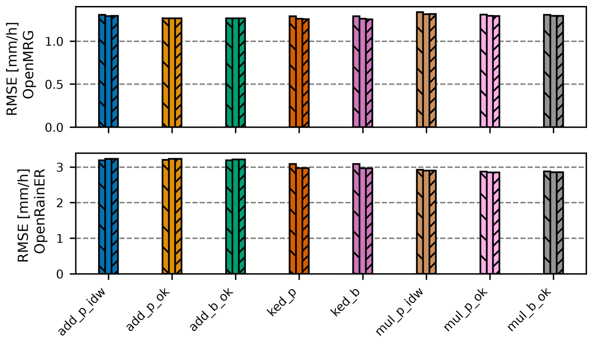
Figure B1 Root Mean Square Error (RMSE) for all merging methods across three neighborhood size configurations for the OpenMRG (top) and OpenRainER (bottom) datasets. Within each method group, the three bars represent neighborhood sizes of 12, 70, and 500 (all CMLs) in strict left-to-right order. Method acronyms are detailed in Table 1.