Quantifying key parameter sensitivities for water table depth in hydrological schemes of CoLM-PSUADE at a mountain forest site

Accurately representing groundwater dynamics in land surface models (LSMs) is crucial for understanding water-energy cycles and assessing water resources. However, most LSMs lack systematic evaluations of parameter sensitivities governing water table depth (WTD) simulations. This study coupled the Common Land Model (CoLM) with Problem Solving environment for Uncertainty Analysis and Design Exploration (PSUADE) in a single-point framework to facilitate systematic parameter analysis and optimization for improving WTD simulation. The CoLM-PSUADE framework was then applied to evaluate groundwater-related parameters using WTD observations from the Gongga Mountain site. A comprehensive analysis integrating qualitative screening, quantitative validation, and parameter optimization techniques was conducted to evaluate the sensitivities of 56 parameters associated with key hydrological processes and identify their optimal ranges. The results identified eight sensitive parameters in the initial screening, including those controlling unsaturated soil water movement (56-soil_alpha, 53-soil_n), subsurface runoff (40-rsubmax), plant hydraulic processes (49-beta, 45-krmax, 46-ck0), and net surface water infiltration (4-alpha_rain, 10-rhol_nir). Additional experiments with independent random seeds revealed varying sensitivity rankings. In particular, the subsurface runoff parameter r_sub,max exhibited sampling-dependent sensitivity but showed relatively high importance in the analysis. It exhibited a well-defined optimal range (on the order of 10⁻⁴) and regulated both the magnitude of subsurface runoff and its decay with increasing WTD when combined with another empirical parameter in the SIMTOP (Simple TOPMODEL-based) scheme, f_drai, thereby exerting strong control on WTD. The soil hydraulic parameter α showed the highest sensitivity. It regulated unsaturated hydraulic conductivity and soil water retention, thereby exerting a dominant influence on the variability and lagged response of WTD. Based on these findings, a stepwise calibration strategy was recommended, in which the subsurface runoff parameters (r_sub,max and f_drai) are first adjusted to constrain the mean WTD, followed by optimization of other key parameters, such as α, to improve the temporal dynamics of WTD. This study demonstrated that CoLM-PSUADE provides a useful tool for sensitivity-guided parameter optimization in high-dimensional LSMs and hydrological models.

1 Introduction

Groundwater, as a key component of the hydrological cycle, modulates water and energy balances by regulating soil moisture and evapotranspiration, which in turn affects the climate system and terrestrial ecosystem (Vogelbacher et al., 2024). Hence, groundwater processes of varying complexity are increasingly represented in land surface models (LSMs), such as Variable Infiltration Capacity (VIC; Liang et al., 2003), Noah-MP (Niu et al., 2007; Niu et al., 2011; Yang et al., 2011), Community Land Model (CLM; Gulden et al., 2007; Maxwell and Miller, 2005), and Common Land Model (CoLM; Dai et al., 2019d), all of which simulate land surface processes and land–atmosphere interactions. These developments enable investigations into the important role of groundwater in regulating soil moisture (Akhter et al., 2025), evapotranspiration (Maina et al., 2022), and vegetation dynamics (Gou et al., 2018), as well as in moderating global warming and extreme weather events (Marchionni et al., 2020). In most LSMs, groundwater processes are typically solved within a variably saturated flow framework using pressure head or soil moisture profiles (Dai et al., 2019d; Yang et al., 2026), and are tightly linked with infiltration, runoff, and evapotranspiration processes (Jia et al., 2026). In addition, new modules such as plant hydraulics (Kennedy et al., 2019; Li et al., 2021) or new parameterizations of the soil water characteristic curve (Silwimba et al., 2025) have been progressively integrated into LSMs to investigate coupled interactions between water cycles and atmospheric feedback. Against this backdrop, LSMs have continued to evolve, with developments such as CoLM2004 (Dai et al., 2003), CoLM2014 (Dai et al., 2019a), and CoLM2024 (Bai et al., 2024). As a result, the simulation of groundwater dynamics has been increasingly dependent on new parameterization schemes. This trend highlights the need to accurately simulate water table depth (WTD) to better understand and predict groundwater behaviour in a changing climate.

During the model calibration process, parameter uncertainty is widely recognized as one of the greatest sources of uncertainty in process-based LSMs (Raoult et al., 2025). Consequently, the appropriate specification of model parameters is essential for ensuring the accurate representation of land surface processes (Zheng et al., 2019; Tsai et al., 2021). Conventional hydrological modeling typically relies on manual calibration, in which simulated outputs are compared against observations to adjust parameter values. However, as LSMs continue to evolve and increasingly incorporate key components of the hydrological cycle, the energy balance, and biogeochemical processes (Dai et al., 2019b), the number of adjustable parameters has expanded substantially (from O(10) to O(100)) (Li et al., 2013). This growth renders parameter calibration a computationally expensive and time-consuming task, particularly for LSMs characterized by high-dimensional systems, strong nonlinear parameter interactions, and pronounced parameter space heterogeneity. Therefore, identifying the parameters that exert the dominant influence on model outputs is crucial for improving efficiency while maintaining accuracy. By fixing insensitive parameters or those that can be directly observed, the dimensionality of the adjustable parameters can be reduced, thereby lowering computational costs and enabling effective enhancement of model performance. In this process, many parameters without clear physical meaning cannot be directly measured, while they are essentially effective parameters (Raoult et al., 2025), such as empirical parameters used to control subsurface runoff. For these parameters, sensitivity analysis becomes a critical tool for identifying the most influential ones (Ratto et al., 2012). Among available approaches, global sensitivity analysis methods have gained widespread application in nonlinear process-based models because they quantify both individual parameter effects and interaction effects on model outputs (Zhan et al., 2013; Erdal and Cirpka, 2019). Qualitative analysis methods provide intuitive rankings of relative parameter importance with fewer model runs, making them suitable for efficiently screening out insensitive parameters in high-dimensional systems (Guerrero et al., 2017). However, they do not explain how much of the performance variance is due to a given parameter. In contrast, quantitative approaches evaluate the contribution of each parameter to the total output variance, thereby enabling a more rigorous and comprehensive assessment (Gan et al., 2014). Nevertheless, such methods typically require a large number of model runs and thus incur substantial computational costs, especially for complex models with high-dimensional parameter spaces. Therefore, an integrated strategy that combines qualitative screening with subsequent quantitative assessment has increasingly become a common practice (Gan et al., 2014; Li et al., 2013). To further evaluate optimal parameter values, sensitivity analysis is commonly combined with parameter optimization techniques (Duan et al., 1994). In this context, integrated analysis platforms play an increasingly important role. In particular, the Problem Solving environment for Uncertainty Analysis and Design Exploration (PSUADE) software package offers a complete workflow that includes parameter sampling, sensitivity analysis, and parameter optimization (Tong, 2022). PSUADE supports various sampling strategies and analysis methods, thereby enabling effective parameter screening and optimization in complex LSMs.

Previous studies have successfully coupled PSUADE with the CoLM2014 (Li et al., 2013), the NCAR community atmosphere model (Pathak et al., 2020), the Sacramento Soil Moisture Accounting (SAC-SMA) model (Gan et al., 2014), and the Canadian Small Lake Model (CSLM; Guerrero et al., 2017) to evaluate the performance and computational efficiency of various sensitivity analysis methods and sampling strategies. However, these studies have largely focused on sensible and latent heat fluxes (Pathak et al., 2020), net radiation, soil temperature, and soil moisture (Li et al., 2013; Guerrero et al., 2017), while systematic sensitivity analysis targeting WTD remain scarce. Notably, most existing studies focus only on sensitivity analysis and uncertainty quantification, with limited efforts to further integrate parameter optimization based on sensitivity analysis results. Therefore, exploring the combined use of sensitivity analysis and parameter optimization within PSUADE can enable effective parameter estimation and evaluation. This combined approach improves the accuracy of WTD simulations and is of great significance for understanding the dynamic response of WTD to hydrological fluxes within land–atmosphere interactions.

This study aims to improve WTD simulation by coupling CoLM2024 with PSUADE (CoLM-PSUADE). Through the integration of qualitative and quantitative sensitivity analyses, together with parameter optimization, key parameters affecting WTD simulations at the site scale, including those governing infiltration, runoff, evapotranspiration, and freeze–thaw processes, are systematically identified, evaluated, and constrained. These results provide a scientific basis and practical guidance for improving WTD simulation and parameter calibration in LSMs.

2 Data and methods

2.1 Study area and datasets

2.1.1 Study area

In this study, we selected a long-term integrated observation site located in a mature Abies fabri forest in the Gongga Mountain region on the eastern Qinghai-Tibet Plateau (hereafter referred to as the GGF site) as the research domain. The GGF site is situated within the Yangtze River Basin (Fig. 1), at 29°34^′ N and 101°59^′ E, with an elevation of 3100 m. The site was chosen due to its shallow WTD, generally less than 2 m (see Sect. 3.4 for details), which enhances the interaction between key hydrological processes such as infiltration, runoff, evaporation, and freeze–thaw. In such shallow groundwater systems, the water table is located within or close to the rooting zone, and capillary rise can further extend the influence of groundwater into the unsaturated zone (Rohde et al., 2024). This strong coupling between groundwater and hydrological processes allows for a comprehensive sensitivity analysis of WTD on these critical parameters. Shallow groundwater systems, defined as those with WTD <2 m (O'Connor et al., 2019), are widespread globally (Fan et al., 2013), making this site particularly relevant for studying their behaviour.

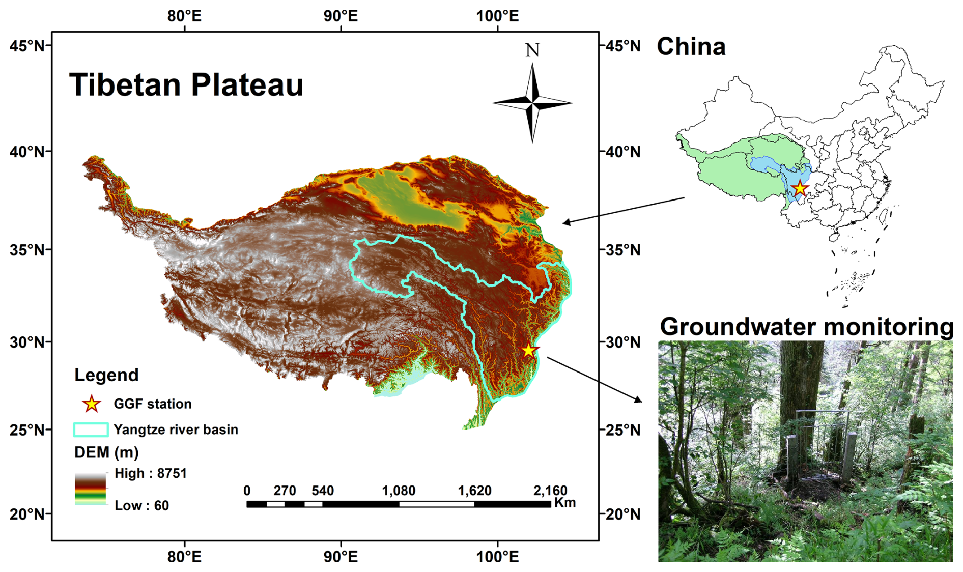
Figure 1 The location and digital elevation model (DEM) of study area (the groundwater monitoring map is reproduced from https://ggf.cern.ac.cn/ent/index, last access: 3 November 2026).

The GGF site is characterized by a cold and humid climate, with a mean annual air temperature of approximately 4 °C and mean annual precipitation of about 1900 mm, most of which occurs between June and September (Zhao et al., 2017). This site, with its mature Abies fabri forest community, represents the typical altitudinal zonal vegetation type found between 2800 and 3600 m in the Gongga Mountain region (Sun et al., 2013; Zhao et al., 2017). The soil is classified as brown coniferous forest soil with the subclass albic brown coniferous forest soil. Soil texture characterization was based on the measured particle size compositions at five depth intervals (0–10, 10–20, 20–40, 40–60, and 60–100 cm), which were collected on 25 August 2005 and 27 September 2015 (Table 1; Yang et al., 2020). As the particle size fractions were determined according to the United States Department of Agriculture (USDA) classification system, which defines sand (0.05–2 mm), silt (0.002–0.05 mm), and clay (<0.002 mm), the soil texture classification was consistently interpreted using the USDA system. Accordingly, the soil was predominantly identified as loamy sand or sandy loam, exhibiting a relatively uniform vertical distribution throughout the profile (Fig. 2).

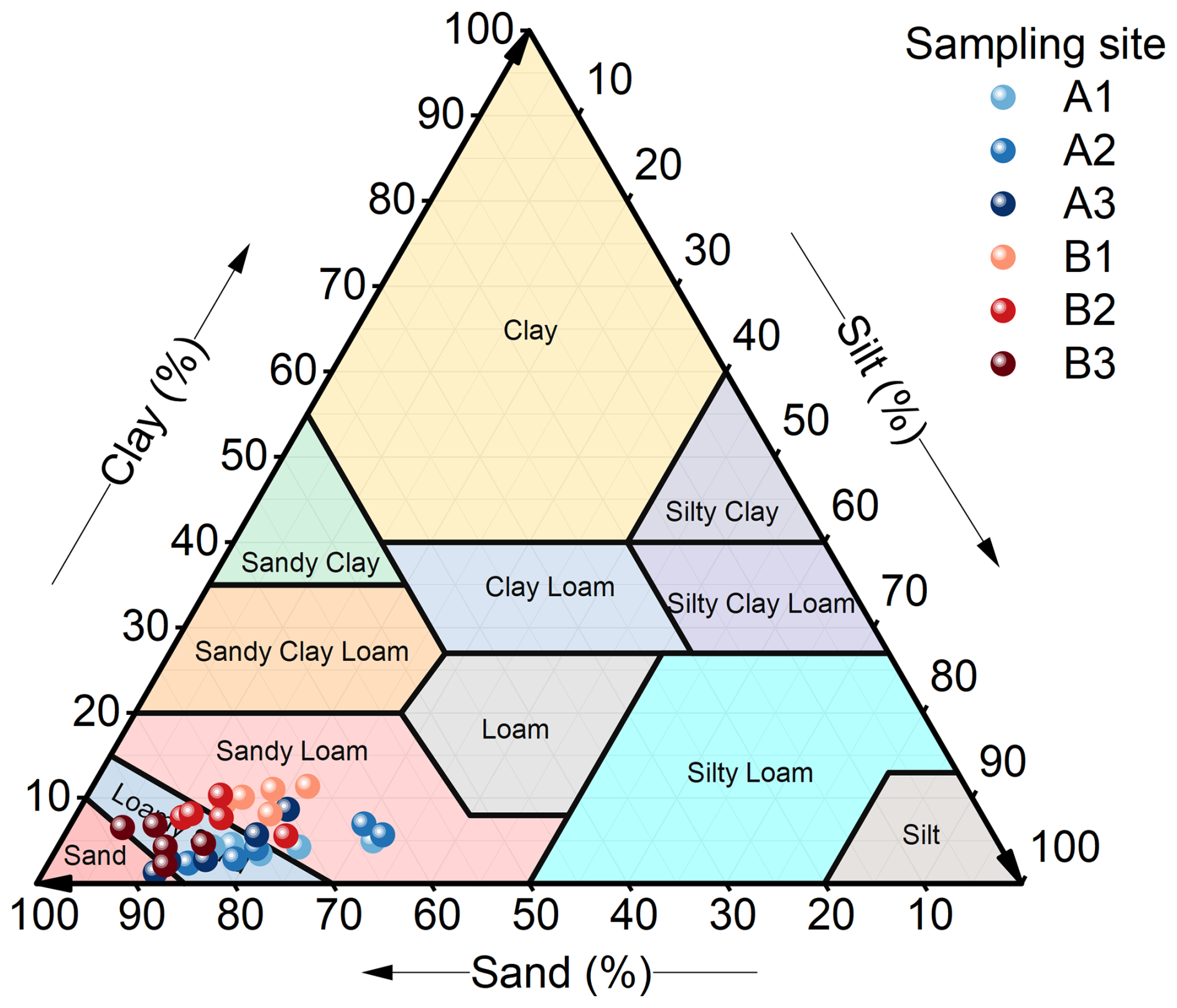
Figure 2 The soil texture classifications for samples collected at the GGF site in 2005 (A1, A2, A3) and 2015 (B1, B2, B3). A and B represent different sampling years, while 1, 2, and 3 denote three distinct plots. Each sampling point contains five measurements, representing soil depths of 0–10, 10–20, 20–40, 40–60, and 60–100 cm.

The CoLM-PSUADE was used to conduct sensitivity analysis and parameter optimization for WTD simulation, providing insights into the coupled hydrological processes at this representative site.

2.1.2 Forcing data and validation data

The forcing and validation data are summarized in Table 1. Meteorological forcing for CoLM was obtained from the meteorological forcing dataset for the Third Pole (TPMFD), including precipitation, 2 m air temperature, 2 m specific humidity, 10 m wind speed, near-surface air pressure, downward longwave radiation, and downward shortwave radiation (Jiang et al., 2025, 2023; Shao et al., 2022). Soil hydrothermal parameters were sourced from the Global Soil Dataset for Earth System Modeling (GSDE; Dai et al., 2019c; Shangguan et al., 2014a), which provides bulk density, thermal conductivity, volumetric and gravimetric fractions of soil particles, and key parameters of the van Genuchten model. The dataset is vertically discretized into eight layers corresponding to depths of 0–0.045, 0.045–0.091, 0.091–0.166, 0.166–0.289, 0.289–0.493, 0.493–0.829, 0.829–1.383, and 1.383–2.296 m (Dai et al., 2019c). Leaf area index (LAI) data were derived from the reprocessed MODIS Version 6.1 LAI dataset (Yuan et al., 2011; Lin et al., 2023). WTD measurements at the GGF site were sourced from the dataset of groundwater levels in the Chinese Ecosystem Research Network (CERN; Zhu et al., 2017b). The simulation periods were assigned different purposes for spin-up, sensitivity analysis, parameter optimization, and long-term validation of the optimized parameter set. The sensitivity analysis covered the 2005–2007 period, whereas the parameter optimization and validation covered the longer 2005–2014 period. Specifically, the model was spun up during 2005–2006 to achieve a dynamically equilibrated state, after which the 2006–2007 period was used for sensitivity analysis and parameter optimization. The selected 2006–2007 period exhibited relatively representative WTD dynamics at the GGF site while maintaining computational feasibility for the repeated sensitivity experiments. The temporal generalization of optimized parameters was subsequently validated using the simulation spanning 2007–2014, which included diverse hydroclimatic conditions for further evaluation of model performance. Additional discussion on the representativeness of the selected period is provided in Sect. S1 in the Supplement.

Table 1 The datasets used in this study.

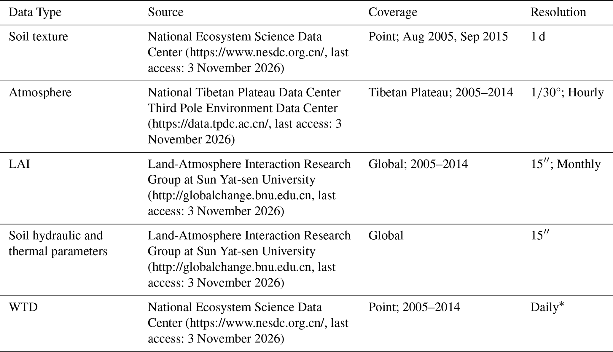
^∗ WTD observations were recorded at irregular intervals ranging from 1–9 d, with most measurements spaced 4–6 d apart. During model evaluation, simulated WTD values were matched with the corresponding observation dates.

2.2 CoLM-PSUADE coupling framework

2.2.1 PSUADE

PSUADE software package, first released in 2007 and developed by Charles Tong, has been widely used for over 18 years and provides a comprehensive suite of tools for uncertainty analysis, sensitivity analysis, response surface analysis, and parameter optimization (Tong, 2022, 2016). Notably, PSUADE is well suited for models with a large number of parameters and complex parameter interdependencies.

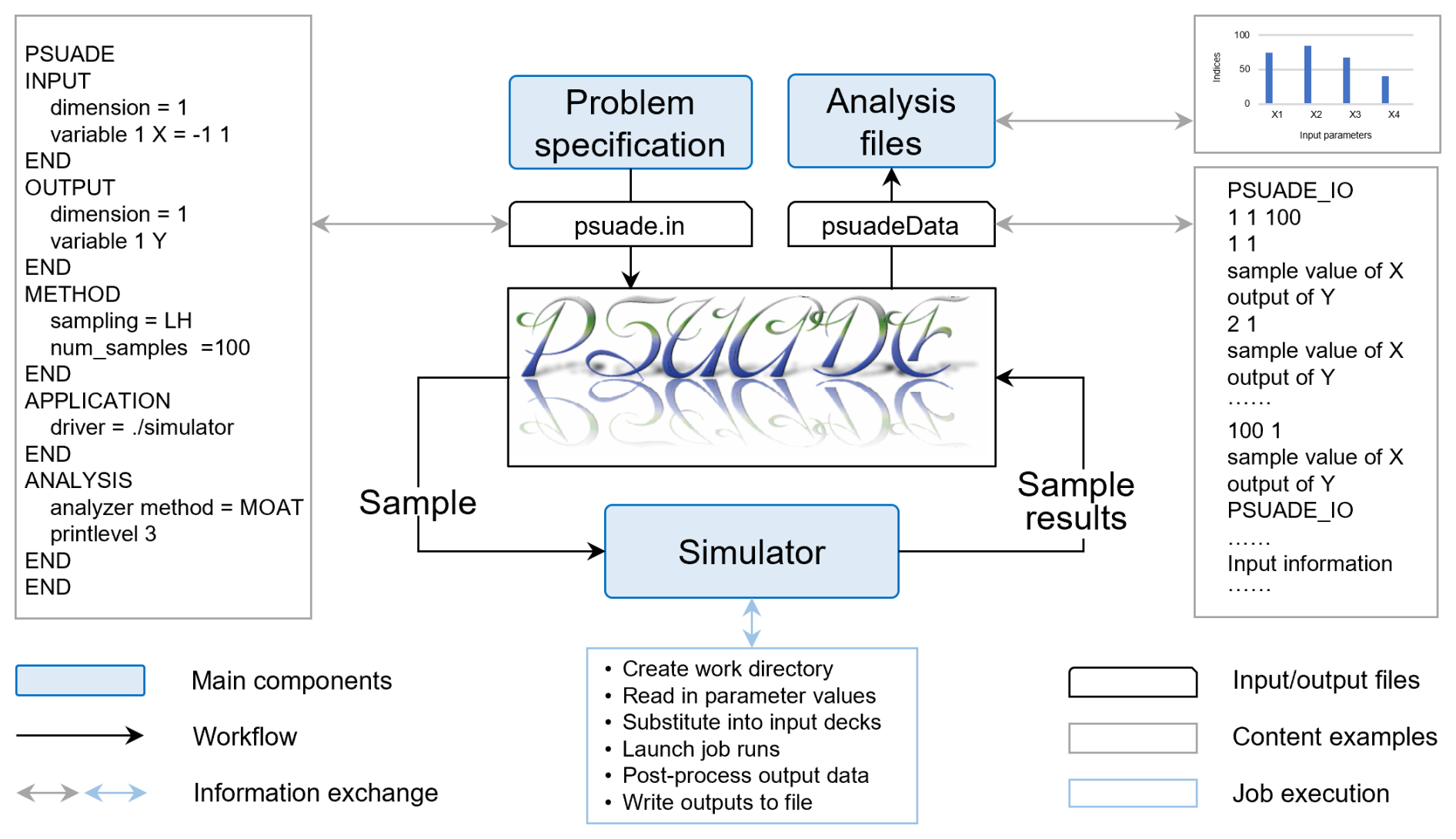
Figure 3 Execution framework of PSUADE (modified from https://www5.in.tum.de/~neckel/siamuq18_slides_minisymp/2018_PSUADE_Tong.pdf, last access: 3 November 2026).

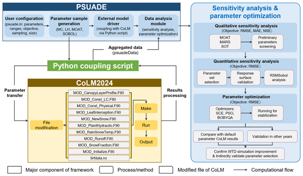
Core components of PSUADE include the sampling module, a simulator execution environment, and the analysis module (Fig. 3). The sampling module generates random samples based on user-specified parameters, their ranges, and the number of samples. The simulator execution environment, after the parameter samples have been constructed, propagates these sampled values to the simulator to produce corresponding outputs. The integrated environment in PSUADE enables simulator execution and results collection. In this study, the simulator is implemented as a Python script (Wu et al., 2026). When invoked by PSUADE, this script is responsible for launching CoLM and handling data exchange between PSUADE and CoLM, thereby achieving the coupling. The analysis module then evaluates the relationships between the sampled parameters and the resulting objective functions. In this study, qualitative sensitivity analysis, quantitative sensitivity analysis, and parameter optimization methods were employed (see Sect. 2.3 for details).

2.2.2 CoLM and adjustable parameters identification

CoLM is built upon the foundations of the Bonan LSM (Bonan, 1996), the Biosphere-Atmosphere Transfer Scheme (BATS; Dickinson et al., 1993), and the 1994 version of the LSM from the Institute of Atmospheric Physics, Chinese Academy of Sciences (IAP94; Dai and Zeng, 1997; Dai et al., 2003). It can be applied in both offline mode and coupled configurations with global or regional climate models (Zhang et al., 2025). Following major updates in 2004 and 2014, the model has advanced to the CoLM2024 (Bai et al., 2024). In the latest version, substantial improvements have been implemented in the model grid structure (Huang et al., 2022; Dai et al., 2019b), vegetation subgrid representation (Dai et al., 2019b), and fundamental datasets (Dai et al., 2019a, c). Process parameterizations have also been substantially improved, including surface energy fluxes (Chen et al., 2024), hydrology (Dai et al., 2019d; Zhu et al., 2017a), and human disturbances (Zhang et al., 2025). CoLM2024 has also been successfully coupled with a general circulation model (GCM; Xin et al., 2019).

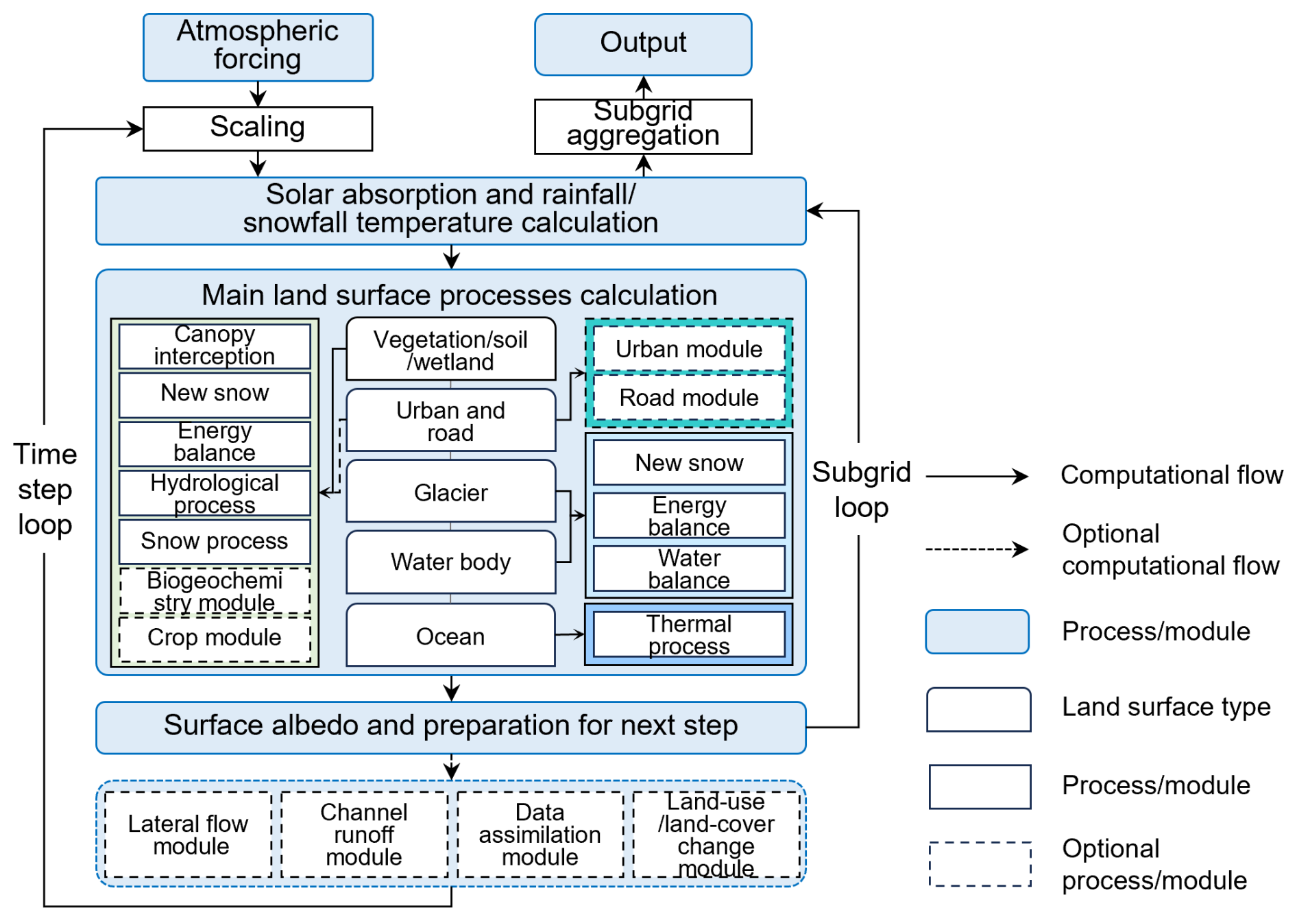
Figure 4 Computational framework of CoLM (modified from https://github.com/CoLM-SYSU/CoLM-doc/, last access: 3 November 2026).

The computational framework of CoLM is illustrated in Fig. 4. The execution of CoLM typically follows a sequential workflow of making surface data, making initial condition data, and executing the main program. Making surface data involves constructing the model grid and subgrid units, as well as aggregating high-resolution raw data to derive surface properties at the model grid scale. Making initial data defines the model's initial states. The main program performs time integration of key land surface processes, including physical, chemical, biological, and anthropogenic processes. When the model is run in offline mode, atmospheric forcing data must be provided as input. In addition, depending on the model configuration, auxiliary inputs such as aerosol, nitrogen deposition, and ozone data may also be required and are read during model execution. The model outputs generally consist of surface property data, model state variables, and historical output data.

When coupled with PSUADE, the execution of CoLM is initiated by the simulator specified within PSUADE, which is implemented as a Python script in this study (Wu et al., 2026). Prior to execution, the script replaces the corresponding parameters in the CoLM source files using the sampled parameter values, after which the model is compiled and executed. The selection of adjustable model parameters is primarily guided by their relevance to WTD simulations, with careful consideration of the strong linkages between the simulation process and key hydrological components such as infiltration, evaporation, runoff, freeze–thaw dynamics, and the vertical movement of soil moisture. Accordingly, a total of 56 key parameters associated with these processes were identified. Their physical meanings, categories, value ranges, and the references for determining these ranges are summarized in Table 2. The parameter categories were determined based on the physical processes, with some classifications adapted from Li et al. (2013). The parameter ranges were determined based on the default parameter values implemented in CoLM, the values reported in previous studies, and the need to provide a broad parameter space for analysis. Therefore, the ranges in Table 2 were interpreted as the parameter space explored in this study rather than as universal physically valid limits.

The key parameterization schemes adopted in CoLM, corresponding to the selection of adjustable parameters, are summarized in Table 3. The SIMTOP runoff scheme was used because it is well suited for large-scale runoff generation (Decker, 2015), thereby facilitating future regional-scale applications. For freeze–thaw processes, the supercooled-water scheme newly implemented in CoLM2024 was activated, while all other parameterizations remained consistent with default settings.

Table 2 Adjustable parameters and their ranges.

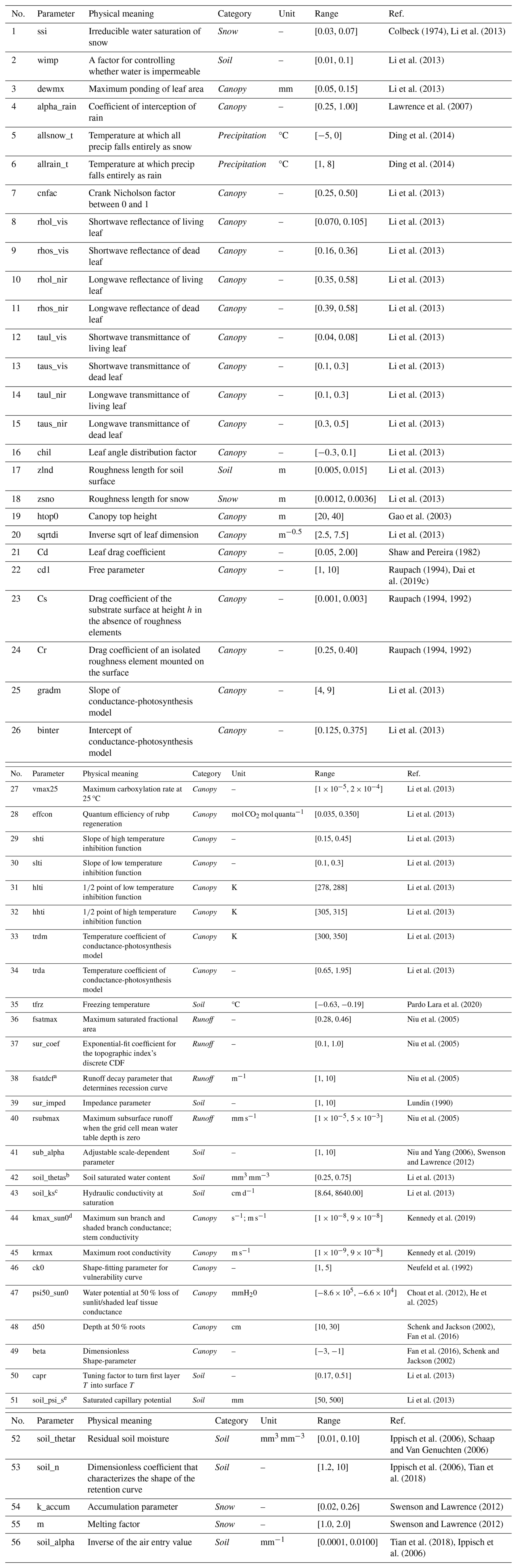
^a Parameter 38 was applied to replace the decay factors in both surface runoff and subsurface runoff calculations. ^b Parameter 42 was also used to update porosity values. ^c For parameter 43, unit conversion was performed by converting the original values reported in the literature from mm s⁻¹ to cm d⁻¹; ^d Parameter 44 simultaneously updates the maximum conductance of sun branch, shaded branch, and stems. ^e Parameter 51 is prescribed as a fixed small value in the new model version. Variations in this parameter have negligible effects on model outputs and are therefore serve as an indirect check within the sensitivity analysis.

Table 3 Summary of key parameterization schemes configured in CoLM.

In the simulations, CoLM was operated at a 30 min temporal resolution on a water-year basis, where a water year is defined from 1 October to 30 September of the following year. Because the TPMFD is provided in coordinated universal time (UTC), the water-year configuration was also specified in UTC time. For simulations spanning both 2005–2007 and 2005–2014, the 2005–2006 water year was consistently repeated 10 times as a spin-up period to ensure the model reached dynamic equilibrium. The subsequent years (i.e. 2006–2007 or 2006–2014) were then used for model evaluation and analysis. The spin-up behaviour of WTD is illustrated in Fig. 5. The spin-up period of 10 years (n=10) satisfies the criterion that the difference in annual mean WTD between two consecutive spin-up years is less than 0.1 % of the annual mean (Hu et al., 2023), as expressed in Eq. (1):

$$\begin{array}{}\text{(1)}& \left|{\text{Var}}^{n+\mathrm{1}}-{\text{Var}}^n\right|<\mathrm{0.001}\cdot \left|{\text{Var}}^n\right|,\left(\mathrm{1}\right)\end{array}$$

where n is the year for spin-up, Var is the variable (i.e. WTD), and the spin-up values are the ratios of the variable difference to the annual mean.

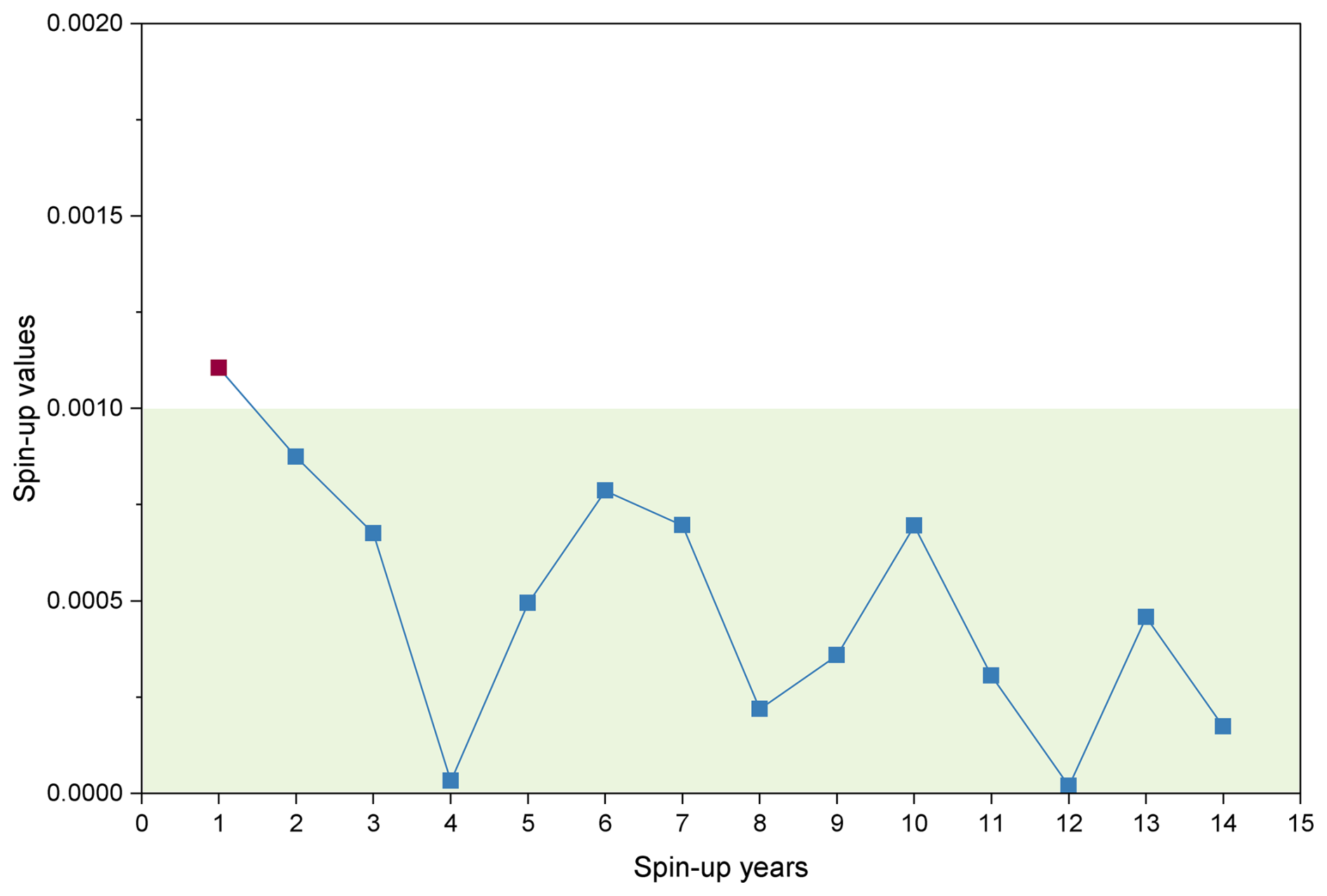
Figure 5 The model spin-up process for WTD, which pass the spin-up test when the curves fall into the green areas.

2.2.3 CoLM-PSUADE coupling framework

Coupling between CoLM and PSUADE was implemented by a Python-based linking script (Wu et al., 2026). Within this coupling framework, PSUADE is employed to randomly generate input parameter sets, control the execution of CoLM simulations through the linking script, and perform subsequent data analysis. CoLM is used to simulate the corresponding WTD for each input parameter set. The linking script served as an interface to transfer input parameters from PSUADE to CoLM and return analysis metrics calculated from the CoLM simulation results back to PSUADE.

The detailed procedure is shown in Fig. 6. Firstly, the PSUADE input file (psuade.in) is configured to include key settings (such as the number of parameters, their ranges, the objective function, the sampling method, and the sample size) and the designation of a driver script for coupling with the external model (i.e. CoLM). Secondly, a custom script is developed to sequentially perform a series of tasks, including reading the sampled values of the 56 parameters, replacing the corresponding default values in the CoLM source files, compiling and executing CoLM, post-processing simulation outputs to calculate objective function values, and writing the aggregated results to the PSUADE output file (psuadeData). This procedure is repeated iteratively until the number of runs reaches the prescribed sample size. Subsequently, the built-in statistical methods in PSUADE are employed to analyze the relationships between parameter combinations and the evaluation metrics. Finally, the internal data analysis modules of PSUADE enable further investigations, such as statistical characterization of input-output relationships, sensitivity analysis, response surface construction, and parameter optimization.

Figure 6 Coupling framework of CoLM-PSUADE.

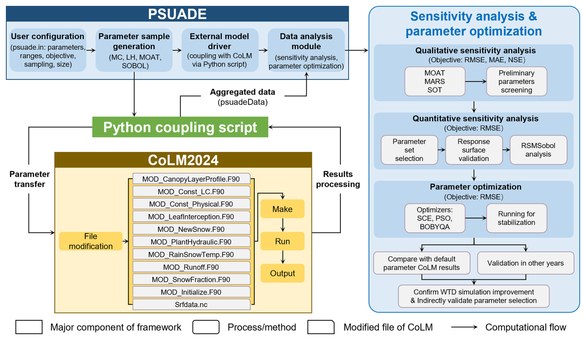
2.3 Sensitivity analysis and parameter optimization

2.3.1 Sensitivity analysis methods

Sensitivity analysis often combines multiple analytical methods to screen sensitive parameters, particularly during the qualitative screening stage (Gan et al., 2014; Li et al., 2013). Previous studies have shown that Multivariate Adaptive Regression Splines (MARS) method performs better in identifying insensitive parameters, whereas the Sum-of-Trees (SOT) method is more effective in detecting highly sensitive parameters (Gan et al., 2014). Generally, MARS, SOT and Morris One-At-a-Time (MOAT) method yield comparable screening results (Li et al., 2013). Specifically, the MOAT method evaluates not only the overall importance of input parameters but also their interaction effects (Gan et al., 2014). According to the PSUADE handbook, MOAT is effective when the number of input parameters ranges from 10 to 100. The SOT method performs well with large random sample sizes, while MARS is a low-cost response surface modeling approach. Based on these considerations, this study selected MOAT (Morris, 1991), SOT (Breiman et al., 1984), and MARS (Friedman, 1991) as global sensitivity analysis methods to qualitatively screen 56 parameters. To enable comparison among different methods, all sensitivity indices were normalized. The consistent identification of sensitive parameters among these methods was considered as stronger evidence of parameter importance than the results obtained from a single method.

Following qualitative sensitivity screening, quantitative sensitivity analysis should be performed on the reduced parameter set to assess parameter sensitivity by computing the impact of the parameter on the total variance of model outputs. The Sobol method is often used for this purpose by providing robust variance-based sensitivity measures (Sobol, 1993, 2001). However, it requires a large sample size for high-dimensional problems, leading to high computational cost. To reduce the number of model runs, Sobol analysis can be conducted on a surrogate response surface model. Once the performance of the response surface model is validated, the response surface model-based Sobol method (RSMSobol) can be applied efficiently (Li et al., 2013). Therefore, RSMSobol was employed to validate the results of the qualitative screening in this study. Specifically, the Gaussian Process (GP) response surface model was adopted following the recommendations in the PSUADE and previous studies demonstrating its superior performance in approximating complex model responses (Gong et al., 2015).

A comprehensive description of these methodologies, including their theoretical principles, min-max normalization, and response surface validation metrics, is provided in Appendix A.

2.3.2 Sampling methods and sample size

Based on the work of Li et al. (2013) and Gan et al. (2014), Monte Carlo (MC) and Latin Hypercube (LH) sampling were adopted for the SOT and MARS methods, respectively. In addition, the MOAT and SOBOL methods utilized their inherent sampling schemes, respectively. Regarding sample size, Li et al. (2013) concluded that sensitive parameters can be effectively screened when the sample size is 10 times the total number of parameters. Therefore, four sampling sizes, corresponding to 5, 10, 15, and 20 times the total number of parameters, were adopted to evaluate the qualitative sensitivity analysis results comprehensively. For quantitative sensitivity analysis, model runs were set between 20 and 150 times the number of different input dimensions to align with the approximately 1000–3000 runs reported in the studies (Li et al., 2013; Gan et al., 2014; Guerrero et al., 2017). Notably, unlike MARS and SOT, the MOAT and SOBOL methods require (n+1) and (n+2) runs per sample, respectively, where n represents the number of parameters. The detailed experimental design is summarized in Table 4.

Table 4 Experimental design of the sensitivity analysis methods.

All experiments were run on a workstation with a 128-cores AMD EPYC 7C13 processor (2.0 GHz base clock) and 64 GB DDR4 RAM. Each sampling run typically requires approximately 30–40 min.

2.3.3 Objective function

The root mean square error (RMSE), mean absolute error (MAE) and Nash-Sutcliffe Efficiency (NSE) (Duc and Sawada, 2023) of the simulated WTD were adopted as objective functions for analysis. The corresponding equations (Eqs. 2–5) are given as follows.

$$\begin{array}{}\text{(2)}& {\displaystyle }\text{RMSE}=\sqrt{{\displaystyle \frac{\mathrm{1}}{N}}\sum _{i=\mathrm{1}}^N{\left(O_i-S_i\right)}^{\mathrm{2}}},\text{(3)}& {\displaystyle }\text{MAE}={\displaystyle \frac{\mathrm{1}}{N}}\sum _{i=\mathrm{1}}^N\left|O_i-S_i\right|,\text{(4)}& {\displaystyle }\text{NSE}=\mathrm{1}-{\displaystyle \frac{\sum _{i=\mathrm{1}}^N{\left(O_i-S_i\right)}^{\mathrm{2}}}{\sum _{i=\mathrm{1}}^N{\left(O_i-\stackrel{\mathrm{‾}}{O}\right)}^{\mathrm{2}}}},\text{(5)}& {\displaystyle }\stackrel{\mathrm{‾}}{O}={\displaystyle \frac{\mathrm{1}}{N}}\sum _{i=\mathrm{1}}^N{O}_i,\end{array}$$

where N is the number of data points, O_i and S_i denote the observed and simulated values at the ith time step, respectively, and $\stackrel{\mathrm{‾}}{O}$ is the mean of observed values.

When calculating these evaluation metrics, model outputs originally recorded in Coordinated Universal Time (UTC) are first converted to local time, after which daily mean values are computed. The resulting daily averages were then temporally aligned with the observations, and the evaluation metrics are finally calculated based on the aligned data.

2.3.4 Parameter optimization

In this study, parameter optimization was performed on the previously screened sensitive parameters to reduce model complexity and mitigate computational costs (Gong et al., 2015). This sequential design was used not only to estimate reasonable parameter combinations but also to provide an independent evaluation of the effectiveness of the selected sensitive parameters. Specifically, after identifying the stable sensitive parameters through qualitative screening and quantitative verification, optimization and validation were conducted to examine whether adjusting these parameters could effectively improve WTD simulations. The optimization methods within the PSUADE framework were selected based on a comprehensive evaluation of the problem types (global or local), variable types (continuous, discrete, or categorical), and range constraints of variables. Consequently, Shuffled Complex Evolution (SCE), Particle Swarm Optimization (PSO), and Bound Optimization BY Quadratic Approximation (BOBYQA) were identified as suitable optimizers for bound-constrained continuous variables, with RMSE serving as the objective function. As the primary goal of the optimization was to demonstrate the validity of the identified sensitive parameters by enhancing WTD simulation accuracy, the comparison was restricted to results obtained within a fixed number of runs. Specifically, three optimization methods were compared within about 500–1000 runs, a duration during which the RMSE reached and maintained a stable state. The SCE and BOBYQA methods were evaluated for 1000 objective-function evaluations, whereas the PSO method included only 496 valid evaluations due to an unexpected interruption caused by a power outage at the workstation during the additional experiment. In addition, LH sampling was employed due to its effective stochastic properties, which allow for superior optimization performance even with smaller sample sizes (Gong et al., 2015). This characteristic ensures the feasibility of using the stable minimum RMSE attained within 500–1000 runs as the final evaluation index. Then, the parameter combination corresponding to the lowest RMSE was fed back into the CoLM to generate optimized WTD time series, which were then compared against the baseline results obtained using default parameters. The specific principles of the selected optimization methods are summarized in Appendix B.

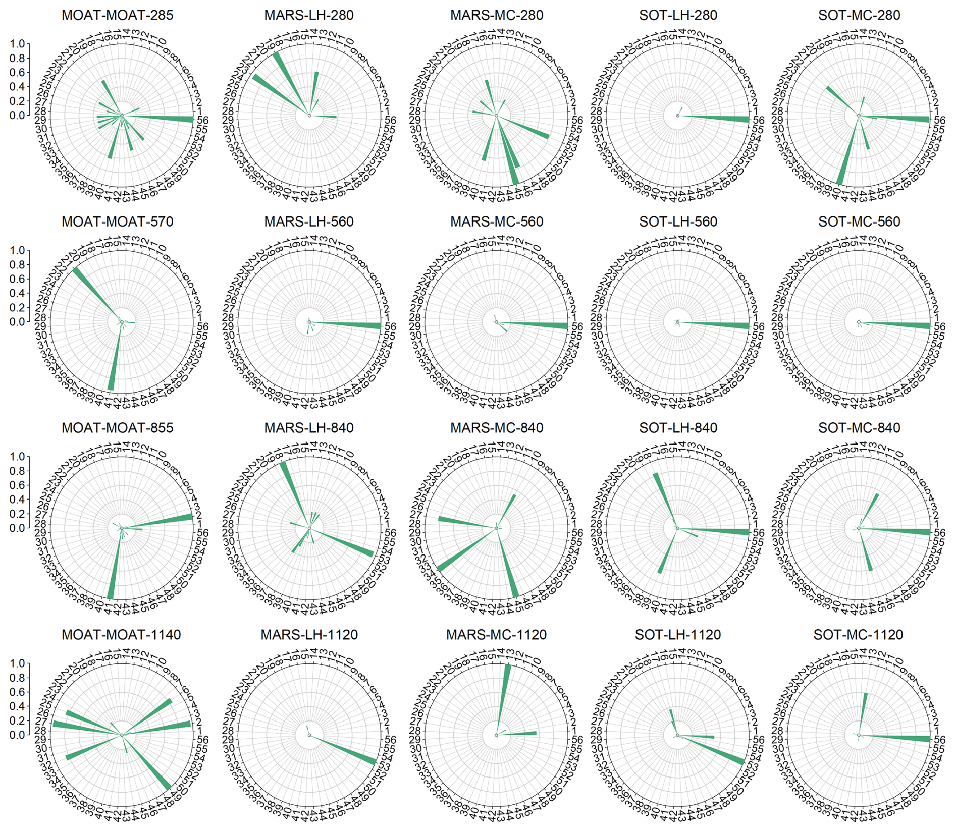
Figure 7 Qualitative sensitivity analysis results based on the RMSE objective function. The numbers on the outer ring represent parameter indices (refer to Table 2 for the corresponding parameter definitions). The length of each pointer indicates the normalized sensitivity index, ranging from 0 to 1, with longer pointers denoting higher sensitivity. Each subplot title follows the format “sensitivity analysis method–sampling technique–sample size”.

3 Results

3.1 Qualitative parameter screening

Qualitative sensitivity scores for 56 parameters across the MOAT, MARS, and SOT methods, obtained using different sampling techniques and sample sizes relative to the RMSE objective function, are shown in Fig. 7. In the figure, longer pointers indicate higher parameter sensitivity. Notably, only the MARS and SOT methods consistently identified the same highly sensitive parameter (56-soil_alpha) at the sample size of 560. In other cases, results exhibited significant discrepancies in ranking. This variability indicated that sensitivity conclusions depend strongly on the analysis method and sampling design, and therefore should not be inferred from a single method or solely from the highest sampling level. Although previous studies on soil temperature and soil moisture have often adopted sensitivity results obtained at the maximum sample size (Li et al., 2013), such a practice may not be sufficient for WTD, as the present results revealed pronounced inter-method variability that could mask critical sensitivity information. In addition, the quality of the generated samples was quantitatively evaluated using distance metrics, and detailed validation is provided in Sect. S2.

Based on a cross-method evaluation, the number of significantly sensitive parameters, represented by prominently longer pointers in the radar chart, ranged from 1 to 16. Comparing different sampling techniques (column 2 vs. 3 and column 4 vs. 5) revealed that MC sampling tended to identify a broader set of sensitive parameters than LH sampling at equivalent sample sizes. Furthermore, the sensitive parameters identified using MAE (Fig. S2 in the Supplement) and NSE (Fig. S3) as objective functions were largely consistent with those based on RMSE, except for the MARS-LH-280 and MARS-MC-280 cases. This consistency indicated that the dominant sensitivity structure was largely preserved across different objective functions.

The results were further compared using a heat map (Fig. 8). As the sample size increased, the sensitivities of several parameters changed substantially. Compared with the case where the sample size was five times the total number of parameters, the sensitivities of parameters 1-ssi, 2-wimp, 6-allrain_t, 13-taus_vis, 17-zlnd, 25-gradm, 27-vmax25, 33-trdm, 49-beta, and 53-soil_n increased markedly, whereas those of parameters 22-cd1 and 40-rsubmax decreased. For most parameters, sensitivity exhibited unstable and non-monotonic responses to increasing sample size. In contrast, parameter 56-soil_alpha consistently remained highly sensitive across different sample sizes, with normalized sensitivity values exceeding 0.5 in most cases. Overall, parameter sensitivities varied irregularly with sample size, further highlighting the necessity of jointly analyzing results from multiple experiment designs to robustly identify stably high-sensitivity parameters.

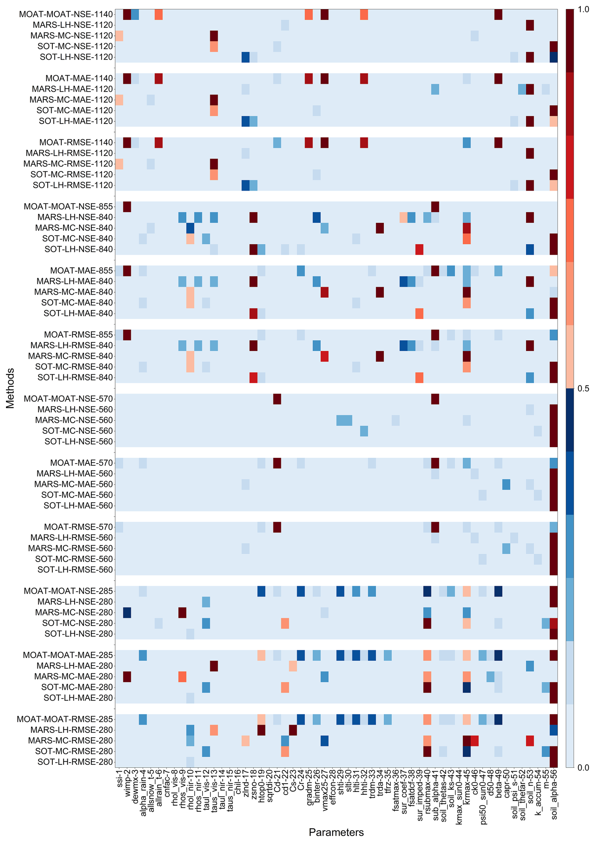
Figure 8 Normalized qualitative sensitivity analysis results (where 1 and 0 represent the most and least sensitive, respectively). The horizontal axis denotes parameter indices, while the vertical axis represents different analysis methods and sampling techniques, following the format “sensitivity analysis method–sampling method–objective function–sample size”.

To ensure a comprehensive sensitivity analysis while accounting for variations in methods, objective functions, and sample sizes, sensitive parameters were selected from two complementary perspectives: (1) integrating different analysis methods and sample sizes under a fixed objective function, and (2) integrating different objective functions and sample sizes under a fixed analysis method.

Taking the first perspective as an example, the screening procedure is described as follows. Based on the earlier radar chart results, the number of notably sensitive parameters ranged from 1 to 16. For each combination of analysis method and sample size, the top 15 parameters in the sensitivity ranking were included in an initial candidate set. These parameters were then sorted primarily by their frequency of occurrence across all combinations, with higher frequency ranked first. In cases of equal frequency, their sensitivity rankings across different results were compared, and the final order was determined by the cumulative ranking value in ascending order. The top 10 parameters in the comprehensive ranking were ultimately identified as highly sensitive parameters. The combined set of highly sensitive parameters obtained under different objective functions constituted the final parameter set for this perspective. Parameters classified as highly sensitive under most objective functions were further regarded as stably sensitive parameters. The second perspective followed a similar procedure: with the analysis method fixed, sensitivity rankings from different objective functions and sample sizes were integrated to derive another set of highly sensitive parameters.

From the perspective of fixed objective functions (Fig. 9), parameter 56-soil_alpha was consistently identified as the most sensitive parameter across all objective functions, demonstrating high stability and significance. Within the set of highly sensitive parameters derived by integrating the screening results of the three objective functions (Fig. 9d), aside from 56-soil_alpha, parameters such as 45-krmax, 4-alpha_rain, 53-soil_n, 49-beta, 10-rhol_nir, 40-rsubmax, and 46-ck0 were also consistently classified as highly sensitive across multiple objective functions and are therefore considered as stably sensitive parameters. In contrast, parameters 19-htop0, 42-soil_thetas, 2-wimp, and 1-ssi were identified as highly sensitive under only one or two objective functions and are thus regarded as unstable highly sensitive parameters.

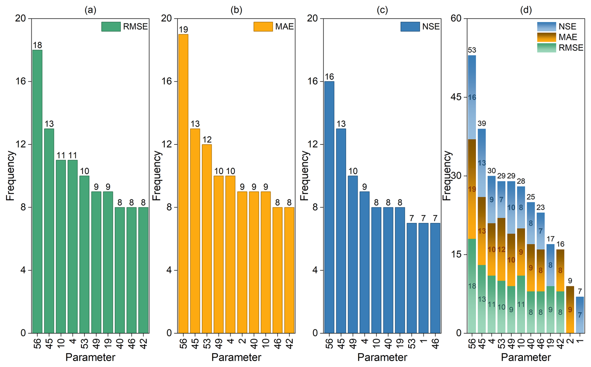
Figure 9 Highly sensitive parameters identified across various methods and sample sizes under different objective functions. The horizontal axis denotes parameter indices, while the vertical axis represents the frequency of occurrence. Labels above the bars indicate the total frequency for each parameter. Subplots (a)–(c) display the 10 most frequently identified sensitive parameters under the RMSE, MAE, and NSE objective functions, respectively. Subplot (d) shows the integrated results of (a)–(c), where labels within the bars indicate the frequency counts for each specific objective function.

From the perspective of fixed analysis methods (Fig. 10), parameter 56-soil_alpha remained the most sensitive parameter. In addition to 56-soil_alpha, 45-krmax was the only parameter identified as the most sensitive across all analysis methods. Although the stably sensitive parameters selected under this perspective differed from those obtained under the previous perspective, parameters 53-soil_n, 10-rhol_nir, 49-beta, 4-alpha_rain, and 40-rsubmax followed 45-krmax in descending order of frequency. Parameter 46-ck0 ranked relatively lower, preceded by parameters 42-soil_thetas, 18-zsno, 24-Cr, and 13-taus_vis.

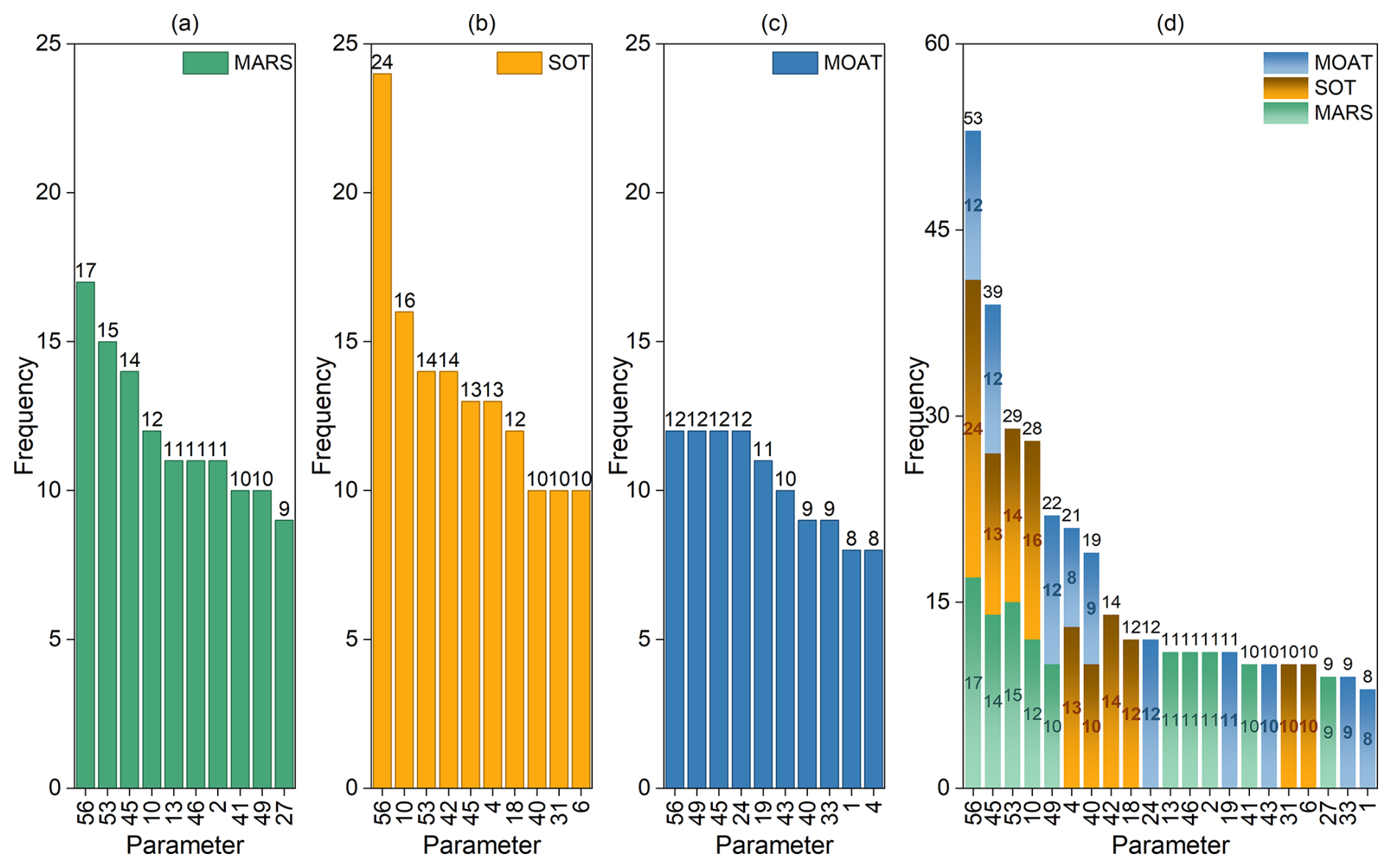
Figure 10 Highly sensitive parameters identified across various objectives and sample sizes under different sensitivity analysis methods. The horizontal axis denotes parameter indices, while the vertical axis represents the frequency of occurrence. Labels above the bars indicate the total frequency for each parameter. Subplots (a)–(c) display the 10 most frequently identified sensitive parameters under the MARS, SOT, and MOAT analysis methods, respectively. Subplot (d) shows the integrated results of (a)–(c), where labels within the bars indicate the frequency counts for each specific analysis method.

Based on the comprehensive ranking results from the two aforementioned perspectives, eight parameters in this screening were identified as stable highly sensitive parameters: 56-soil_alpha, 45-krmax, 4-alpha_rain, 53-soil_n, 49-beta, 10-rhol_nir, 46-ck0, and 40-rsubmax. The remaining highly sensitive parameters were classified as unstable. This process effectively identified key parameters that significantly influence WTD from the total set of 56 parameters. Given that the number of stably sensitive parameters was notably small relative to the total parameter count, the screening procedure demonstrated good applicability for this study.

The aforementioned sensitivity ranking reflected the overall effect of the parameters, while the MOAT method can further reveal the characteristics of parameter interactions. In this approach, the importance of a parameter is indicated by the modified mean (${\mathit{\mu }}_i^{*}$), with larger values indicating higher sensitivity. Meanwhile, the standard deviation (${\mathit{\sigma }}_i^{*}$) characterizes the strength of its interactions, where larger values imply stronger interactions with other parameters. Therefore, in the scatter plots of $\left({\mathit{\mu }}_i^{*},{\mathit{\sigma }}_i^{*}\right)$, parameters that are clearly separated from the main cluster, typically with large ${\mathit{\mu }}_i^{*}$ and ${\mathit{\sigma }}_i^{*}$, can be identified as sensitive. Their distribution further facilitates analysis of the relationship between parameter sensitivity and interaction strength. Taking the experiment with a sample size of 285 as an example (Fig. 11), parameter 56-soil_alpha exhibited the maximum values for both ${\mathit{\mu }}_i^{*}$ and ${\mathit{\sigma }}_i^{*}$, indicating that it was not only the most sensitive parameter but also the one with the strongest interaction effects. For other sensitive parameters, although interaction strength generally increased with sensitivity, certain exceptions were observed. For instance, the sensitivity rankings of parameters 45-krmax, 19-htop0, and 40-rsubmax followed the order $\mathrm{40}>\mathrm{19}>\mathrm{45}$ (Fig. 11a), whereas their interaction strengths followed the order $\mathrm{45}>\mathrm{19}>\mathrm{40}$. In other words, the most sensitive parameter among them exhibited the weakest interactions, suggesting that higher sensitivity does not necessarily imply stronger interactions. Under other sample sizes (Figs. S4–S6), similar non-monotonic relationships between sensitivity and interaction strength were observed, further confirming the sample dependence of qualitative results and the necessity of comprehensive multi-perspective analysis.

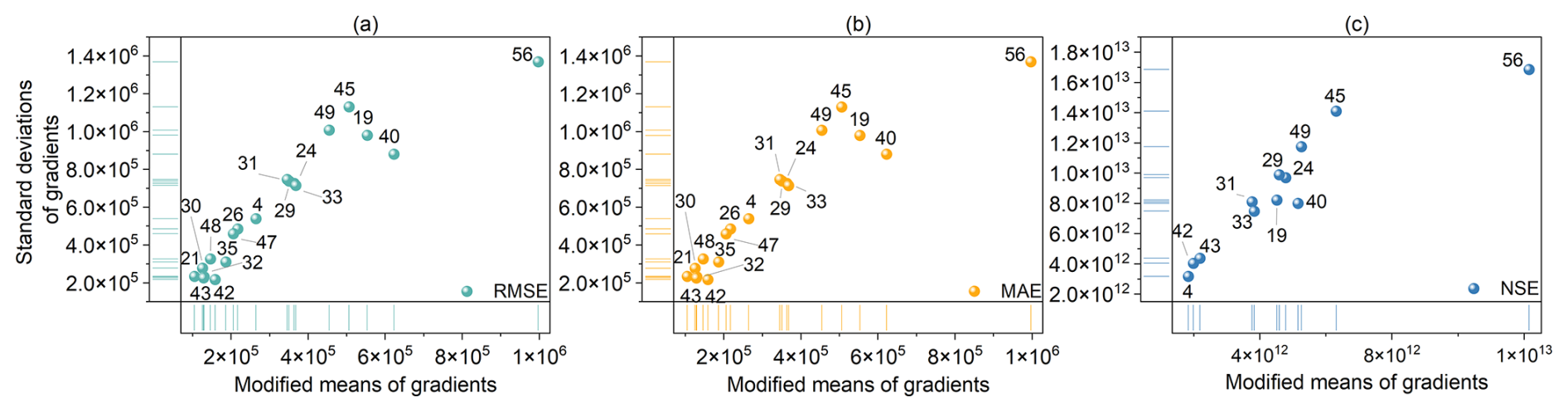
Figure 11 Sensitivity and interaction results from the MOAT method with a sample size of 285. The horizontal axis denotes the modified mean (${\mathit{\mu }}_i^{*}$), and the vertical axis denotes the standard deviation (${\mathit{\sigma }}_i^{*}$). Subplots (a)–(c) correspond to the RMSE, MAE, and NSE objective functions, respectively.

3.2 Quantitative validation of key sensitivity parameters

To validate the eight stably sensitive parameters influencing WTD identified through the previous multi-perspective comprehensive screening, the RSMSobol method was employed for quantitative sensitivity analysis. This approach, based on response surfaces, accounted for varying input dimensions and sample sizes. The Sobol' total-order indices (TSI) reflect the overall influence of each parameter on the objective function, where higher TSI values indicate a more significant impact on the output.

Using all 56 parameters as inputs would lead to high dimensionality and substantial computational cost. Moreover, most response surface analysis methods are recommended for input dimensions below 20. Therefore, three parameter sets with different input dimensions (8, 12, and 21) were selected for analysis: the stably sensitive parameters (8 parameters), the sensitive parameters obtained from fixed-objective-function screening (12 parameters), and the sensitive parameters obtained from fixed-analysis-method screening (21 parameters). Detailed experimental configurations are provided in Table 5.

Table 5 Experimental design of the RSMSobol method.

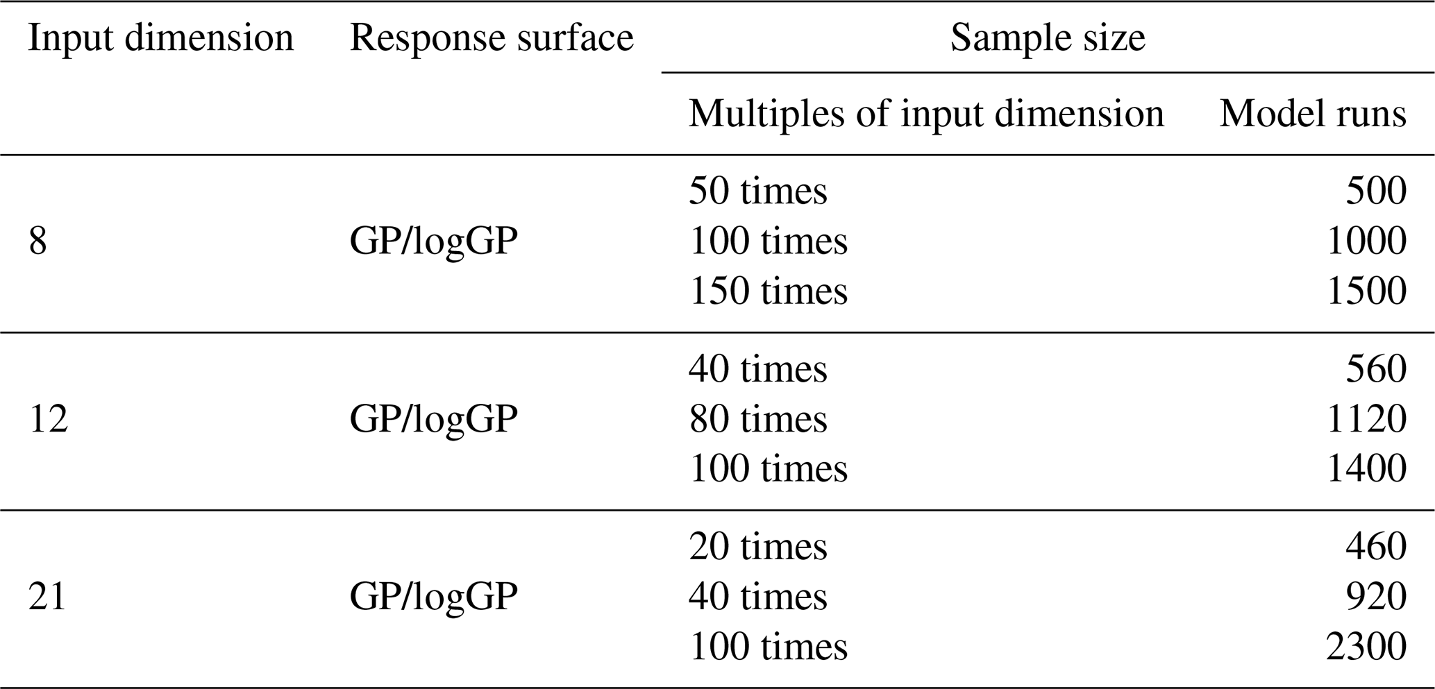
Because the earlier qualitative sensitivity analysis showed consistent sensitivity structures across different objective functions, only RMSE was used as the objective function in the RSMSobol quantitative analysis. A GP was used as the response surface model in all experiments. Additionally, due to the wide range of RMSE (Table S2 in the Supplement), RMSE was log-transformed (natural logarithm) in PSUADE, and a GP-based response surface was then constructed using the transformed data for quantitative analysis, hereafter referred to as logGP. Detailed validations of response surface models are provided in Sect. S3.

In the quantitative sensitivity analysis for an input dimension of 8 (corresponding to the set of stably sensitive parameters; Fig. 12), parameter 56-soil_alpha exhibited a significantly higher TSI than the other parameters, contributing individually 31 %–72 % to the relative importance. This was consistent with its stable and pronounced sensitivity observed in the qualitative sensitivity analysis. Among the remaining parameters, 53-soil_n, 49-beta, 45-krmax, 40-rsubmax, and 4-alpha_rain also showed relatively high sensitivity (Fig. S10). Across experiments with different sample sizes, the cumulative TSI proportion stabilized after 2–7 parameters, reaching values above 90 %. Compared with GP, the cumulative proportion based on logGP tended to stabilize more rapidly.

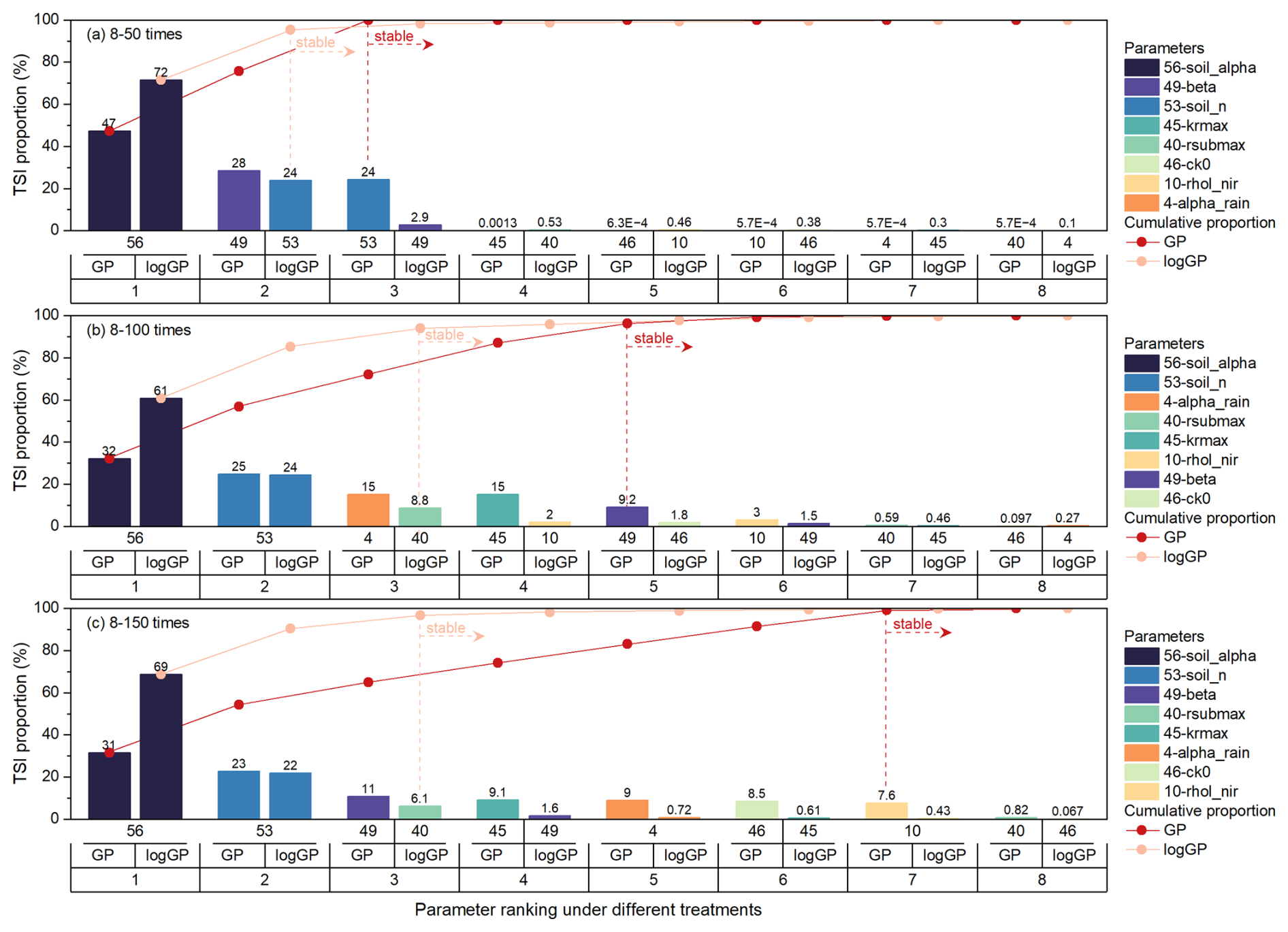
Figure 12 Quantitative sensitivity ranking for an input dimension of 8 (corresponding to the number of stably sensitive parameters). The vertical axis denotes the relative importance based on TSI. The horizontal axis displays the parameter number, response surface method, and ranking number (from top to bottom). The curves represent the cumulative relative importance of parameters, ranked in descending order of importance. Note: “8–k times” in the subplot title denotes an experiment with 8 input parameters and a sample size equal to k times the number of parameters.

When the input dimension is 12 (corresponding to the set of sensitive parameters obtained from fixed-objective-function screening), the stably sensitive parameters 56-soil_alpha, 53-soil_n, 49-beta, 45-krmax, 40-rsubmax, and 4-alpha_rain still retained high relative importance (Fig. 13). Among them, the relative importance of 56-soil_alpha alone reached 41 %–57 %. In terms of cumulative TSI proportion, the eight stably sensitive parameters accounted for 79 %–89 % of the total. This result further confirmed the reliability of the qualitative sensitivity screening. Other parameters, such as 1-ssi, 19-htop0, and 42-soil_thetas, which, although not classified as stably sensitive, ranked among the top 8 (Fig. S11), explain the slightly lower cumulative TSI proportion. Notably, among the eight stably sensitive parameters, the cumulative importance showed a clear tendency to level off after the first 3–5 parameters.

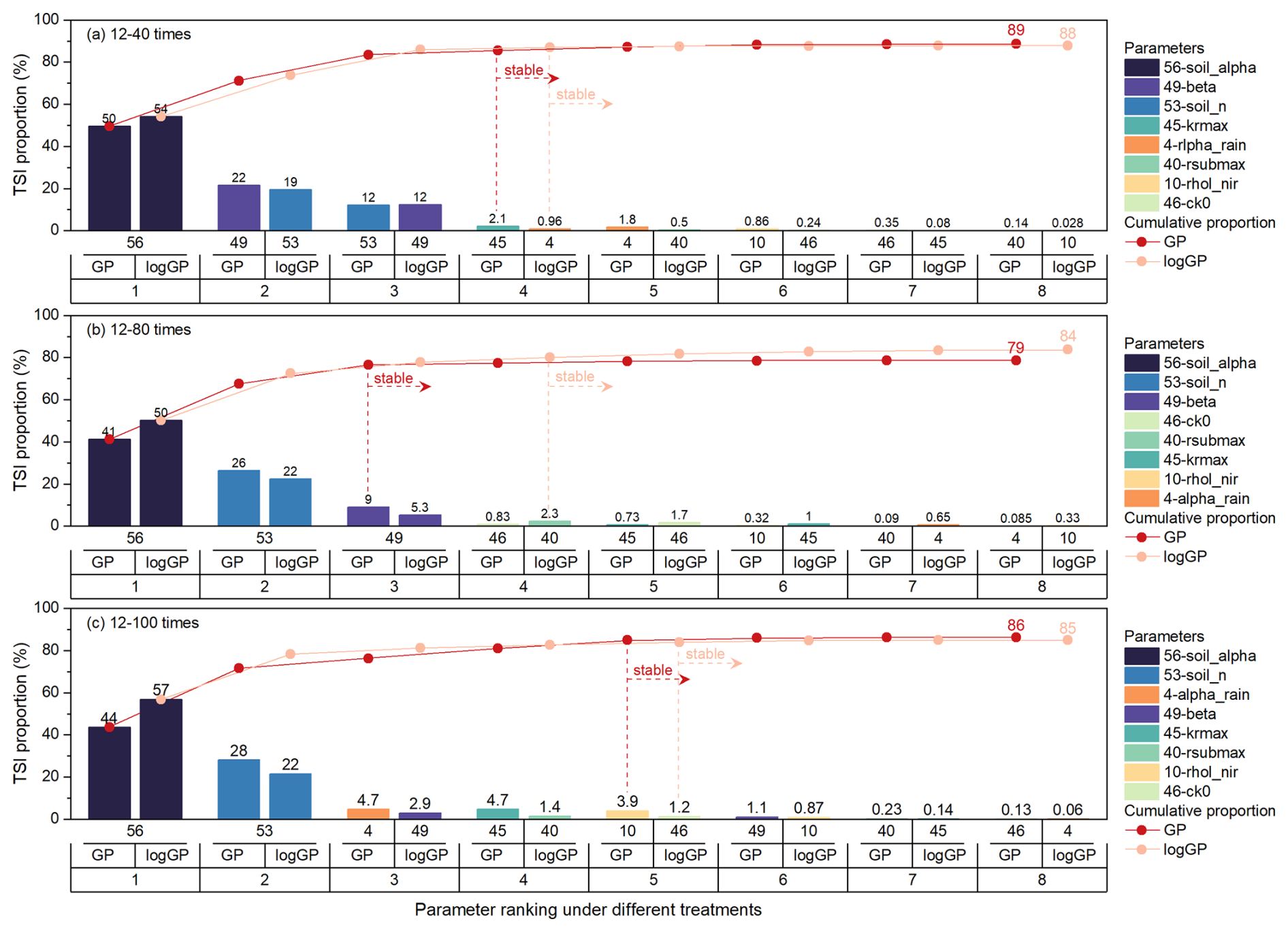
Figure 13 Quantitative sensitivity ranking for an input dimension of 12 (corresponding to the number of sensitivity parameters obtained by screening with fixed objective functions). The vertical axis denotes the relative importance based on TSI. The horizontal axis displays the parameter number, response surface method, and ranking number (from top to bottom). The curves represent the cumulative relative importance of parameters ranked in descending order of importance. Note: “12–k times” in the subplot title denotes an experimental configuration with 12 input parameters and a sample size equal to k times the number of parameters.

When the input dimension was 21 (corresponding to the set of sensitive parameters identified using a fixed screening method), the high-ranking parameters among the eight stably sensitive ones remained concentrated on 56-soil_alpha, 53-soil_n, 49-beta, 45-krmax, 40-rsubmax, and 4-alpha_rain (Fig. 14). Among these, the relative importance of 56-soil_alpha alone accounted for 3.3 %–60 %. The cumulative importance of the eight stably sensitive parameters within the total set of 21 parameters was 36 %–77 %, which was lower than that obtained for an input dimension of 12. This decrease was mainly due to the relatively higher rankings of other parameters, such as 6-allrain_t, 43-soil_ks, 31-hlti, 42-soil_thetas, 19-htop0, 1-ssi, 24-Cr, 33-trdm, and 27-vmax25 (Fig. S12). Similarly, the cumulative importance of the eight stably sensitive parameters tended to stabilize after the first 2–5 parameters.

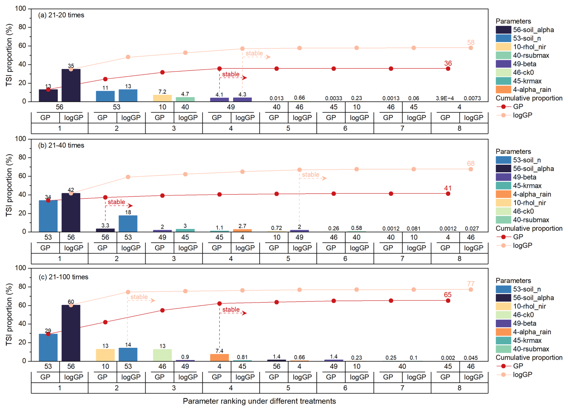
Figure 14 Quantitative sensitivity ranking for an input dimension of 21 (corresponding to the number of sensitivity parameters obtained by screening with fixed screening method). The vertical axis represents the relative importance based on TSI. The horizontal axis displays the parameter number, response surface method, and ranking number (from top to bottom). The curves represent the cumulative relative importance of parameters ranked in descending order of importance. Note: “21–k times” in the subplot title denotes an experimental configuration with 21 input parameters and a sample size equal to k times the number of parameters.

An integrated examination of the quantitative sensitivity analysis results across different input dimensions showed that, as the input dimension increased, the cumulative importance of the eight stably sensitive parameters decreased. This indicated that some non-stably sensitive parameters exerted a non-negligible influence on WTD dynamics in higher-dimensional parameter spaces. Nevertheless, within the stably sensitive parameter set, the importance distribution remained highly concentrated. In particular, 56-soil_alpha, 53-soil_n, 49-beta, 45-krmax, 40-rsubmax, and 4-alpha_rain consistently exhibited dominant contributions across different experimental settings. The subset composed of these six parameters accounted for a cumulative importance close to that of the entire stably sensitive set, indicating that this parameter combination captured the dominant controls on WTD.

3.3 Optimal estimation of key sensitivity parameters

Parameter optimization experiments were performed based on the eight stably sensitive parameters identified in the previous screening to minimize the RMSE of the simulated WTD, aiming to determine the optimal parameter combination and its reasonable value ranges. It should be noted that, within a limited set of 500–1000 optimization runs, the primary purpose of performing parameter optimization was to indirectly validate the effectiveness of the parameter screening process by comparing model performance before and after optimization.

A comparison of the SCE, PSO, and BOBYQA methods revealed clear differences in their convergence characteristics and optimization performance (Fig. 15). In terms of overall behaviour (Fig. 15a), most RMSE values obtained by the SCE method were concentrated between 0.4 and 1 m, with occasional sharp peaks corresponding to failed solutions. The low- RMSE range was stable across evaluations. For the PSO method, RMSE values were primarily clustered between 0.6 and 0.9 m and exhibited evident high-frequency oscillations across evaluations when multiple particles were simultaneously searched. The BOBYQA method showed a markedly different changing pattern. Specifically, during the first 90–140 evaluations, RMSE values fell into the relatively poor range because the change of trust region. However, after approximately 200 evaluations, RMSE remained stable within the range of 0.5–1.0 m. Regarding optimization performance (Fig. 15b), SCE found a better solution during the early stage. As the number of evaluations increased, population of parameter sets evolved in the solution space were progressively constrained to good-quality zones. Ultimately, the SCE method achieved the lowest RMSE value of 0.419 m, demonstrating the best overall performance. Although the RMSE obtained by PSO exhibited considerable variability, its fluctuation range remained within a reasonable interval (0.5–1.2 m), and it was able to identify an optimal solution (0.531 m) within the early stage of the optimization process (around the first 50 evaluations), suggesting relatively fast initial exploration capability. The minimum RMSE obtained by BOBYQA was 0.517 m, lying between the results of the other two methods. The cumulative minimum RMSE curves exhibited relatively stable over the respective evaluation ranges of the three methods, although the comparison was conducted under unequal computational budgets (1000 evaluations for SCE and BOBYQA and 496 valid evaluations for PSO). Overall, SCE outperformed PSO and BOBYQA in terms of the speed of identifying the best solution and the minimum RMSE achieved, indicating that it is more suitable for parameter optimization in the CoLM under present experimental configuration.

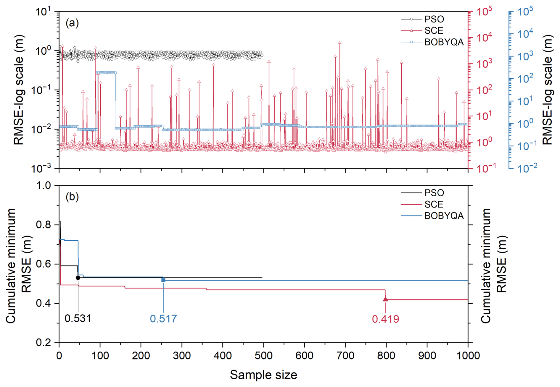
Figure 15 Evolution of (a) RMSE and (b) cumulative minimum RMSE with the number of evaluations for the SCE (1000 runs), PSO (496 runs), and BOBYQA (1000 runs) optimization methods. The vertical axis for subplot (a) is displayed on a logarithmic scale to accommodate the wide range of RMSE values. The vertical axis for subplot (b) represents the lowest RMSE value obtained up to each model evaluation during the optimization process.

Based on the comparison of simulated WTD time series (Fig. 16), the optimal parameter set derived from the SCE method successfully captured the average temporal patterns of the observed WTD. In contrast, the simulations obtained using the PSO and BOBYQA methods showed a systematic overestimation. This result further highlighted differences in parameter search capability among the three optimization methods.

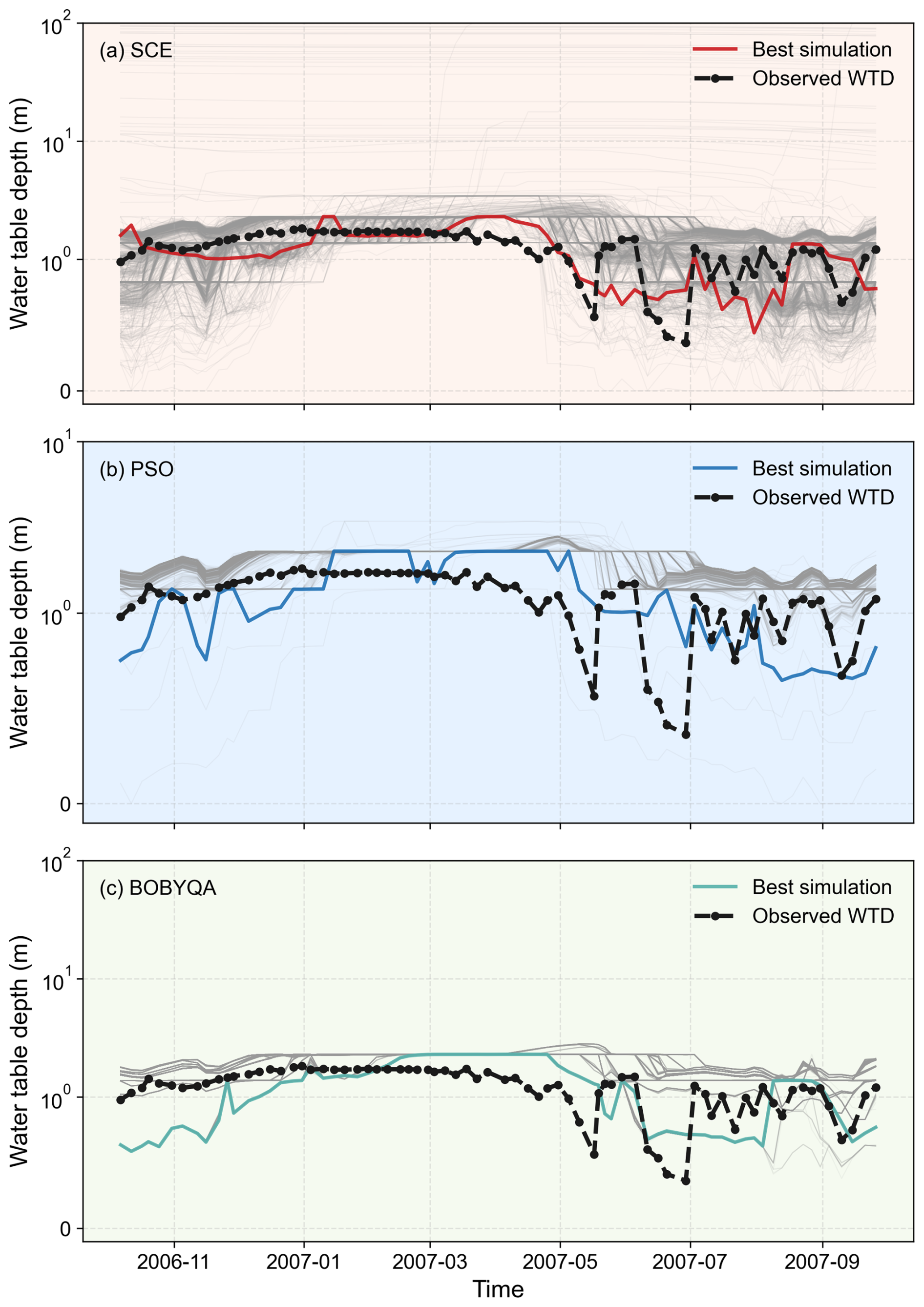
Figure 16 Comparison between observed WTD and simulated time series generated by (a) SCE, (b) PSO, and (c) BOBYQA optimization methods after 1000, 496, 1000 evaluations, respectively. The vertical axis is displayed on a symlog scale to accommodate the wide range of values. The grey lines in the background show the simulation results excluding the best run.

To further analyze the distribution characteristics of parameters associated with favourable solutions, the top 20 % of samples ranked by RMSE from low to high (hereafter referred to as low-RMSE samples) and their associated parameter sets were selected for kernel density estimation (KDE) analysis. The KDE results (Fig. 17) showed that, for the SCE method, the parameter distributions of the low-RMSE samples were markedly more concentrated than those of the full sample set, indicating that optimal solutions were confined to specific parameter ranges. In particular, parameters 40-rsubmax (Fig. 17c) and 56-soil_alpha (Fig. 17h) exhibited the most pronounced convergence. The optimal values of 40-rsubmax were primarily clustered at the order of 10⁻⁴, whereas those of 56-soil_alpha were mainly distributed between 10⁻³ to 10⁻². In contrast, for the PSO method (Fig. S13), the distributions of favourable solutions showed minimal deviation from those of the full sample set for most parameters, except for the parameter 40-rsubmax, suggesting a relatively limited optimization capability. The BOBYQA method (Fig. S14) failed to sufficiently explore the parameter space within 1000 evaluations.

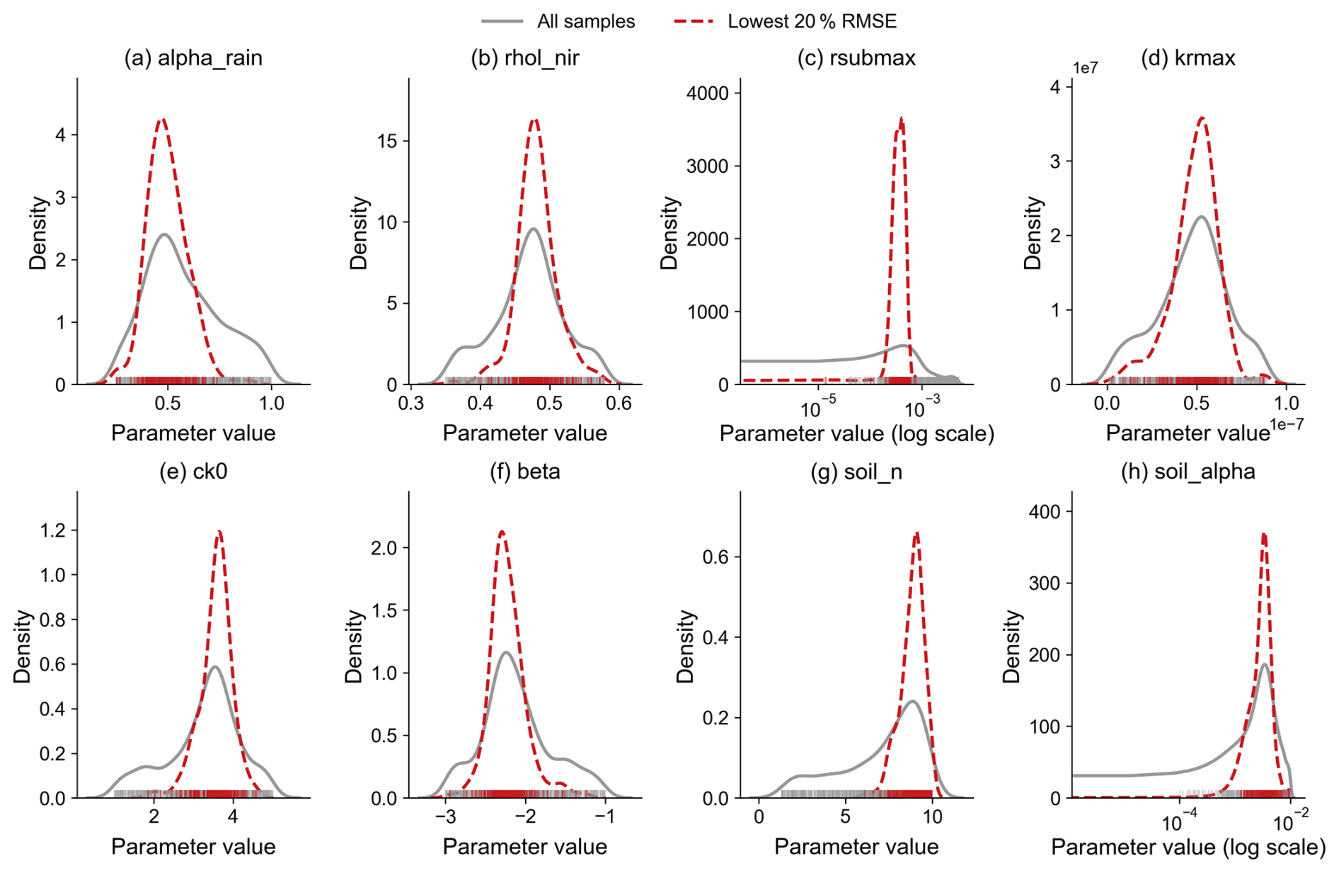
Figure 17 Comparison of KDE for the top 20 % low- RMSE parameter sets (red) versus the entire set of 1000 evaluations (grey) obtained by the SCE method: (a) alpha_rain, (b) rhol_nir, (c) rsubmax, (d) krmax, (e) ck0, (f) beta, (g) soil_n, and (h) soil_alpha. Note that the horizontal axes for rsubmax and soil_alpha are plotted on a logarithmic scale to better visualize their distributions.

The scatter plots of RMSE against parameter values further revealed the influence of key parameters on the optimization outcomes. For the SCE method (Fig. 18), parameter 40-rsubmax (Fig. 18c) exhibited a clear V-shaped pattern in its relationship with RMSE, suggesting a well-defined optimal region. A similar feature appeared as a distinct branching pattern in the PSO method (Fig. S15). In contrast, no obvious trend was observed for the BOBYQA method (Fig. S16), likely due to its limited exploration of the parameter space. These results demonstrated that WTD simulations in the CoLM were highly sensitive to parameter 40-rsubmax. Consequently, constraining this parameter to its optimal range prior to fine-tuning the remaining parameters could significantly improve simulation accuracy.

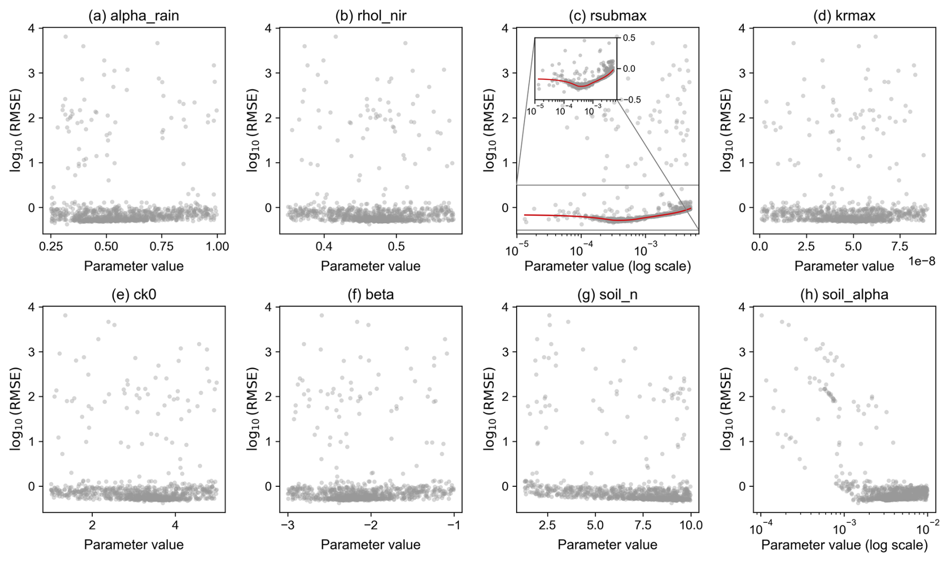
Figure 18 Scatter plots of RMSE against parameter values based on 1000 evaluations obtained during the SCE optimization process: (a) alpha_rain, (b) rhol_nir, (c) rsubmax, (d) krmax, (e) ck0, (f) beta, (g) soil_n, and (h) soil_alpha.

Based on the optimal parameter combinations (Table 6), only three of the eight stably sensitive parameters, namely 56-soil_alpha, 45-krmax, and 40-rsubmax, exhibited order-of-magnitude changes relative to their default values, further highlighting their pivotal roles in WTD simulations. The optimal parameter set obtained from the SCE method markedly improved the WTD simulation, reducing the RMSE by 68 %, with simulated values clustering more closely around the 1:1 diagonal (Fig. 19). The PSO and BOBYQA methods achieved improvements of 59 % and 60 %, respectively. It is worth noting, however, that pronounced “horizontal bands” were evident in the scatter plots both before and after optimization, where the simulated WTD remained nearly constant while the observed WTD varied. This phenomenon primarily occurred during the freeze–thaw period, indicating that the representation of freeze–thaw processes and their interactions with groundwater in the CoLM warrants further investigation.

Table 6 Comparison of the default and optimized values for the eight stably sensitive parameters.

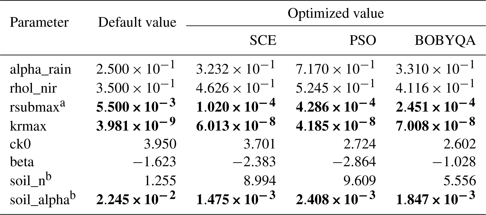
^a Default values represent the original parameter settings implemented in CoLM and are provided as the baseline for comparison. The optimized values were obtained by searching within the parameter ranges specified in Table 2. For rsubmax, the CoLM default value ($\mathrm{5.500}\times {\mathrm{10}}^{-\mathrm{3}}$) slightly exceeds the prescribed upper bound ($\mathrm{5.000}\times {\mathrm{10}}^{-\mathrm{3}}$), because the latter was manually rounded; ^b The original values of the two parameters are different across the 10-layer soil profile. Here, they are represented as the average values. Bold values indicate changes in the order of magnitude relative to the corresponding default values.

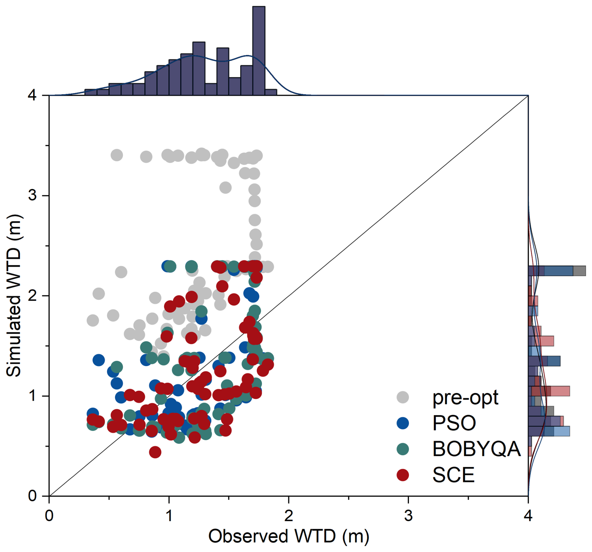
Figure 19 Scatter plots of observed versus simulated WTD using default (before optimization) and optimized parameter sets.

3.4 Validation of the optimized parameters

The preceding analysis indicated that the SCE method achieved the most significant results in parameter optimization. To assess the robustness of the optimized parameters and indirectly validate the effectiveness of the selected parameter set, long-term WTD dynamics at the GGF site from 2005 to 2014 were simulated using the SCE-derived optimal parameter set (i.e. the set corresponding to the lowest RMSE).

A comparison of simulation results across different water years (Fig. 20) revealed that the optimal parameter set derived from the 2006–2007 water year reasonably captured the seasonal and interannual temporal trends of WTD in the subsequent years (2007–2014), with RMSE values ranging from 0.42 to 1.13 m (Fig. 21). The optimized simulations reduced the overestimation and achieved better agreement with observations compared to original simulations. However, although the optimization can enhance the overall simulation, there were still relatively lagging responses in capturing the dynamic changes of WTD (Fig. 20a–c) and abrupt changes or deviations from the observations (Fig. 20c, h). Notably, parameter 40-rsubmax exhibited a distinct turning point in the aforementioned parameter–RMSE scatter relationship. When only this parameter was updated to its optimized value while keeping others at their default values, the RMSE ranged from 0.59 to 0.91 m. The overall simulation value of WTD has improved in this situation and there has been no significant change in the dynamics of WTD.

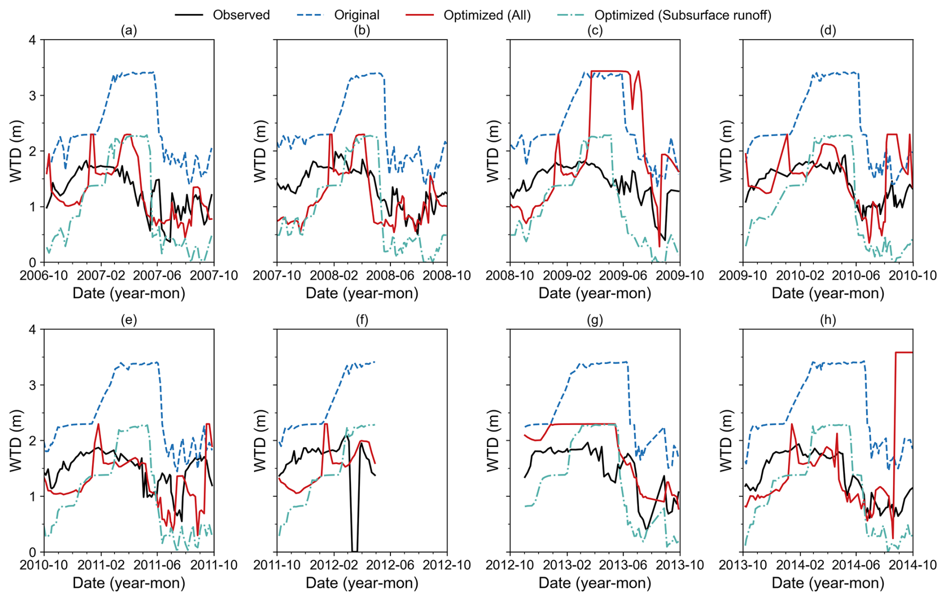
Figure 20 WTD dynamics simulations for the 2006–2014 water years based on the default parameters (blue), the SCE-derived optimal parameter set (red), and the optimized subsurface runoff parameter (40-rsubmax) alone (green).

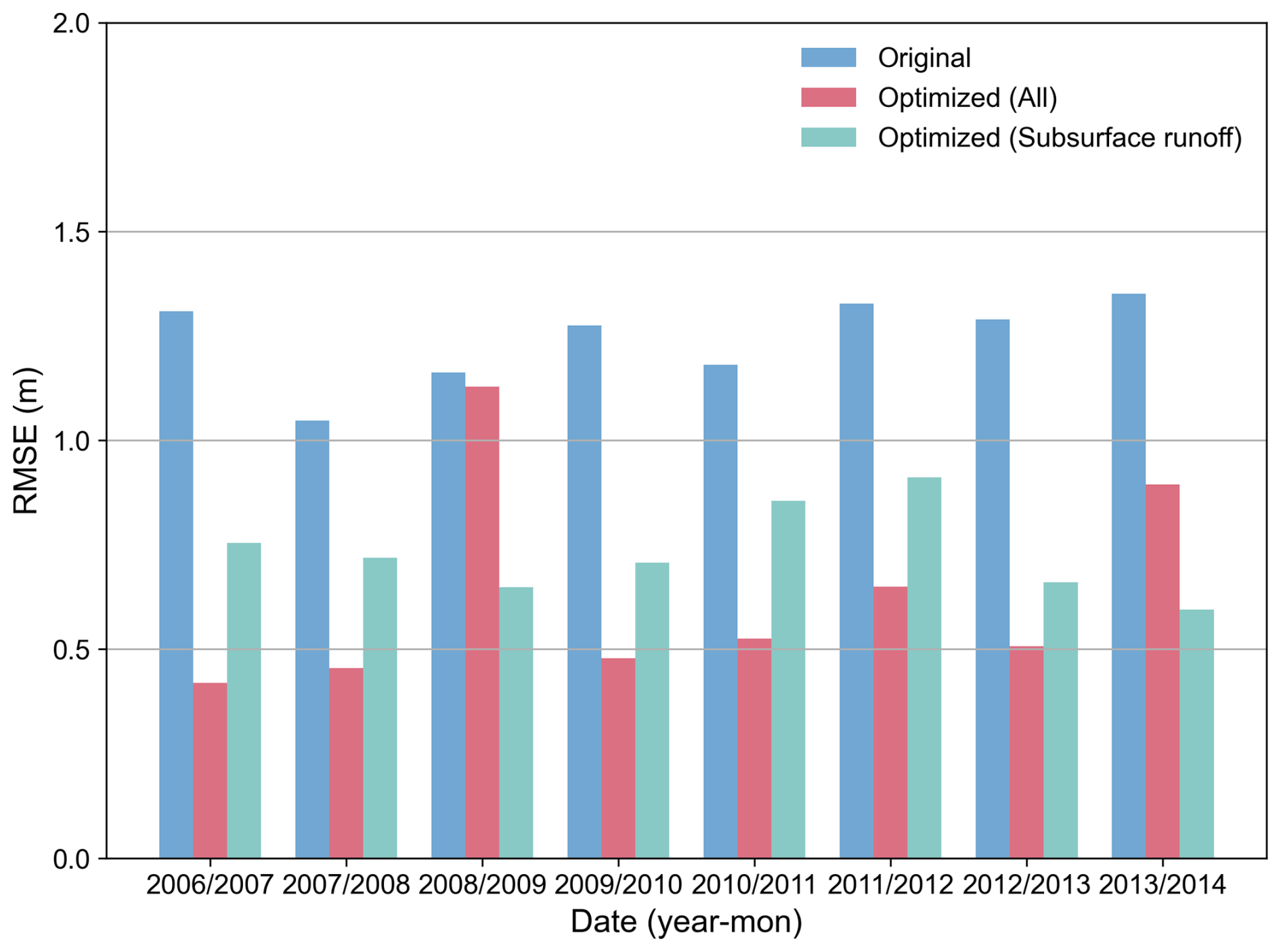
Figure 21 RMSE of simulated WTD across different water years (2006–2014) based on the default parameters (blue), the SCE-derived optimal parameter set (red), and the optimized subsurface runoff parameter (40-rsubmax) alone (green).

In contrast, simulations using the default parameter set yielded higher RMSE values, ranging from 1.05 to 1.35 m (Fig. 21). Regardless of whether the complete optimal parameter set or only the optimized subsurface runoff parameter (40-rsubmax) was used, the RMSE decreased significantly, with reductions of 3 %–68 % and 28 %–56 %, respectively. These results indirectly confirm the effectiveness of the selected parameters.

4 Discussion

4.1 The consistency of the screening results and physical interpretations

The eight stably sensitive parameters identified from the previous screening including 56-soil_alpha, 53-soil_n, 49-beta, 40-rsubmax, 45-krmax, 4-alpha_rain, 46-ck0 and 10-rhol_nir for WTD simulations were comprehensively identified through both qualitative and quantitative sensitivity analyses. The key processes and calculation formulas related to the parameters are detailed in Sect. S5.

From physical interpretations, parameters 56-soil_alpha and 53-soil_n govern the soil-water characteristic curve, where 56-soil_alpha is related to the inverse of the air-entry pressure and 53-soil_n represents the pore-size distribution of the soil (Schaap and Van Genuchten, 2006). By regulating critical thresholds such as field capacity and wilting point, they directly control soil water content in the unsaturated zone, thereby exerting a pronounced influence on WTD dynamics (Muñoz-Vega et al., 2025). The high sensitivity aligns with previous studies, in which both the ISBA land surface model and Hydrus-1D identified these parameters as primary drivers of soil water dynamics (Sobaga et al., 2023; Rezaei et al., 2016). Parameter 40-rsubmax is involved in subsurface runoff parameterization, which characterizes the exponential decay relationship between subsurface runoff and WTD. Physically, 40-rsubmax controls the maximum intensity of subsurface runoff. Changes in this parameter directly alter the equilibrium state of groundwater and consequently influence the simulated WTD. Existing studies have confirmed that this scheme influences the overall depth of WTD (Akhter et al., 2025). Moreover, the critical role of parameter 40-rsubmax itself is also reflected by the distinct turning points observed in the parameter–RMSE scatter plots. Parameter 49-beta controls the root fraction within the soil profile, thereby influencing root distribution and, subsequently, the calculation of soil and root conductance, which determines the plant transpiration rate. Since root distribution is a key factor in groundwater contribution to the root zone, and this contribution occurs when WTD is no deeper than 3.9 to 4.1 m (Zhu et al., 2018), it follows that parameter 49-beta plays a crucial role in modulating WTD. This indicates that root water uptake represents an important pathway linking groundwater dynamics with root water redistribution, particularly in forest ecosystems. Parameters 45-krmax and 46-ck0 are directly involved in computing the hydraulic conductance of plant segments (e.g. leaves, stems, and roots). Field studies have investigated how plants modify hydraulic conductance to maintain water status (Rickard et al., 2025). By modulating transpiration rates, these parameters indirectly regulate water redistribution within soil–vegetation systems and thus influence WTD (O'Connor et al., 2019; Luo et al., 2016). Therefore, their sensitivity reflects the coupling between plant hydrological processes and groundwater dynamics. Parameter 4-alpha_rain is an empirical coefficient representing the interception capacity of the canopy. It is used to estimate throughfall after subtracting canopy interception, thereby determining the net water input reaching the land surface. Rainfall interception loss has been recognized as a vegetation influence on groundwater recharge and consequently on WTD (Fan et al., 2014; Smerdon et al., 2008). Thus, the sensitivity of 4-alpha_rain highlights the importance of accurately representing plant water redistribution processes when simulating groundwater responses. Parameter 10-rhol_nir is used in surface albedo calculations, affecting surface energy balance and snowmelt processes, which indirectly affects infiltration and groundwater recharge. Previous LSM-based studies have reported the direct impact of leaf optical properties on surface solar radiation partitioning (Dong et al., 2021) and the influence of canopy radiation on the dynamics of snowmelt dynamics (Todt et al., 2019).

In summary, the sensitive parameters controlling WTD can be classified into four categories: (1) parameters governing unsaturated water movement (56-soil_alpha and 53-soil_n); (2) those affecting subsurface runoff process (40-rsubmax); (3) those regulating plant hydraulic processes (49-beta, 45-krmax, and 46-ck0); and (4) those determining net surface water input and infiltration (4-alpha_rain and 10-rhol_nir). These sensitive parameters represent different but interconnected hydrological processes within the soil–vegetation–atmosphere system.

4.2 Different roles of subsurface runoff and soil hydraulic parameters in controlling WTD dynamics

Based on the preceding analysis, the subsurface runoff parameter r_sub,max (40-rsubmax) exhibited two key characteristics: (1) a significant turning point in the parameter–RMSE scatter plot during the optimization process, indicating a well-defined optimal parameter range; and (2) the optimization of r_sub,max alone improved the simulations, while avoiding abrupt changes in WTD dynamics. In the SIMTOP parameterization, subsurface runoff is jointly governed by r_sub,max and the decay factor f_drai (i.e. parameter 38-fsatdcfa in Table 2). Although f_drai was initially screened as less sensitive, its synergetic interaction with r_sub,max necessitates a more detailed investigation into their combined influence on WTD.

Optimization results indicated that the optimal r_sub,max was on the order of 10⁻⁴. Consequently, five representative values ($\mathrm{3}\times {\mathrm{10}}^{-\mathrm{4}}$, $\mathrm{4}\times {\mathrm{10}}^{-\mathrm{4}}$, $\mathrm{5}\times {\mathrm{10}}^{-\mathrm{4}}$, $\mathrm{6}\times {\mathrm{10}}^{-\mathrm{4}}$, $\mathrm{7}\times {\mathrm{10}}^{-\mathrm{4}}$) were selected for sensitivity analysis. Within this range of r_sub,max, where subsurface runoff intensity remains reasonable, the decay coefficient f_drai (default value 2.5) was further varied across five levels (1, 2, 3, 4, 5), resulting in 25 parameter combinations (Fig. 22). The results showed that with a fixed r_sub,max, f_drai primarily influenced the mean level, amplitude, and intra-annual variability of the WTD. Lower f_drai values yielded larger seasonal amplitudes and generally deeper WTD. Conversely, increasing f_drai accelerated the decay of subsurface runoff, thereby dampening WTD fluctuations. In contrast, when f_drai was fixed, r_sub,max serves as the primary control for the mean WTD. Higher r_sub,max values resulted in a systematic deepening of the simulated WTD, accompanied by intensified fluctuations in some cases.

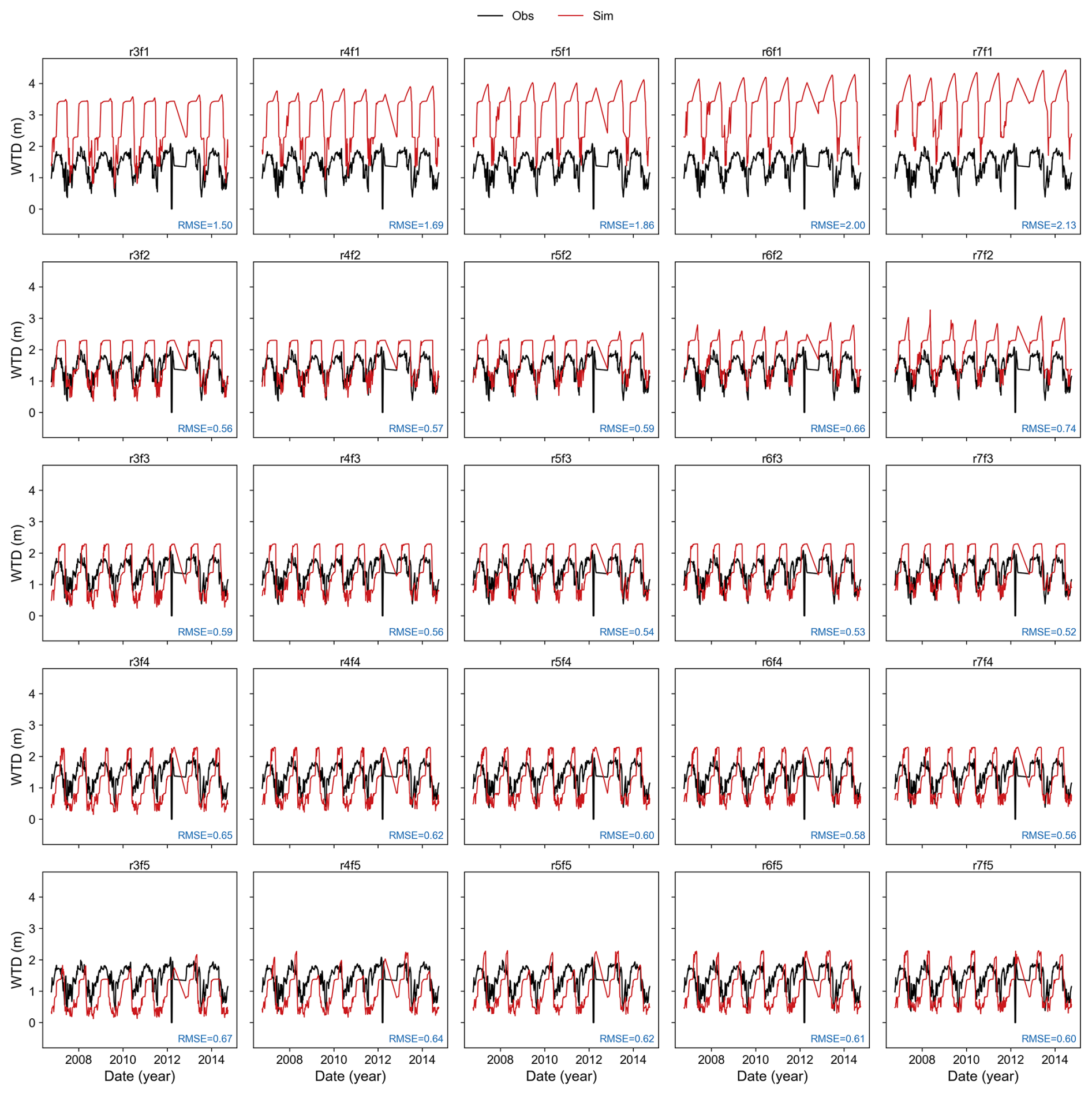
Figure 22 Comparison of observed and simulated daily WTD dynamics across 25 parameter ensembles for the 2006–2014 water years. Each panel is labeled as “rXfY”, where X corresponds to r_sub,max ($\mathrm{3}\times {\mathrm{10}}^{-\mathrm{4}}$, $\mathrm{4}\times {\mathrm{10}}^{-\mathrm{4}}$, $\mathrm{5}\times {\mathrm{10}}^{-\mathrm{4}}$, $\mathrm{6}\times {\mathrm{10}}^{-\mathrm{4}}$, and $\mathrm{7}\times {\mathrm{10}}^{-\mathrm{4}}$) and Y corresponds to f_drai (1, 2, 3, 4, and 5).

Regarding the multi-year average (Fig. 23), when r_sub,max was fixed, the mean WTD decreased markedly (approaches the surface) as f_drai increases. This response was more sensitive at lower parameter values and weakened as f_drai increases further. Conversely, when f_drai was fixed, increasing r_sub,max leaded to a deeper WTD due to enhanced groundwater discharge (Fig. 24). Compared with f_drai, the response of WTD to variations in r_sub,max was relatively moderate within the tested ranges. Specifically, variations in f_drai led to WTD changes exceeding 2 m, while r_sub,max accounted for changes of approximately 1 m. This suggested that once r_sub,max establishes a reasonable runoff baseline, f_drai can further regulate both the mean level and dynamic amplitude of WTD.

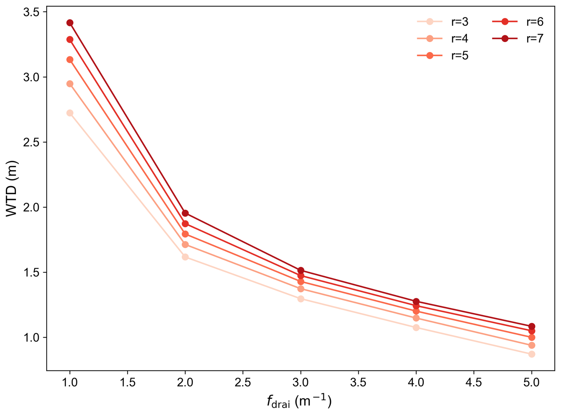
Figure 23 Sensitivity of multi-year mean WTD to the decay factor f_drai under various constant r_sub,max values. The legend labels 3, 4, 5, 6, and 7 correspond to r_sub,max values of $\mathrm{3}\times {\mathrm{10}}^{-\mathrm{4}}$, $\mathrm{4}\times {\mathrm{10}}^{-\mathrm{4}}$, $\mathrm{5}\times {\mathrm{10}}^{-\mathrm{4}}$, $\mathrm{6}\times {\mathrm{10}}^{-\mathrm{4}}$, and $\mathrm{7}\times {\mathrm{10}}^{-\mathrm{4}}$, respectively.

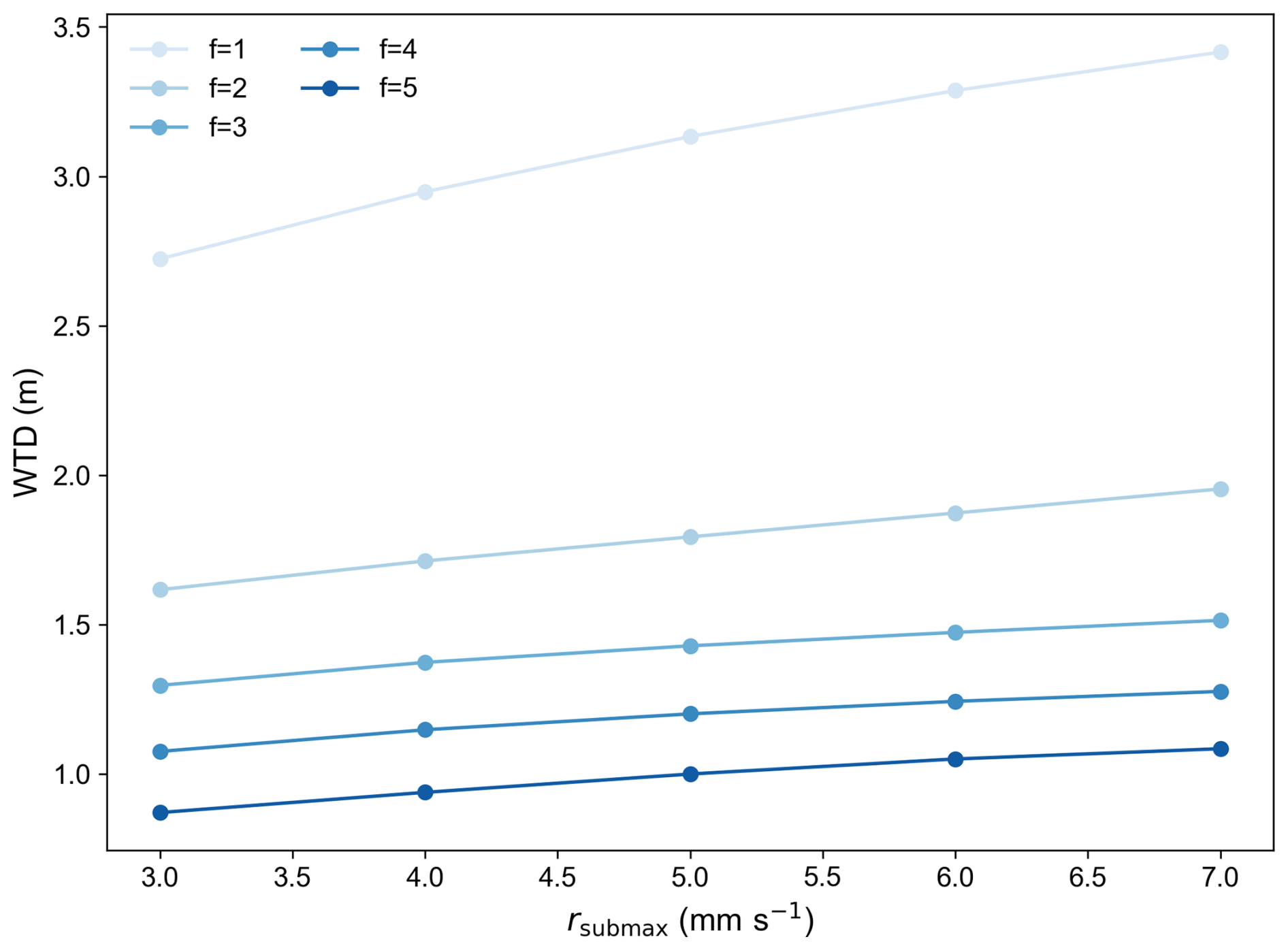
Figure 24 Sensitivity of multi-year mean WTD to r_sub,max under various constant f_drai values. The horizontal axis labels 3, 4, 5, 6, and 7 correspond to r_sub,max values of $\mathrm{3}\times {\mathrm{10}}^{-\mathrm{4}}$, $\mathrm{4}\times {\mathrm{10}}^{-\mathrm{4}}$, $\mathrm{5}\times {\mathrm{10}}^{-\mathrm{4}}$, $\mathrm{6}\times {\mathrm{10}}^{-\mathrm{4}}$, and $\mathrm{7}\times {\mathrm{10}}^{-\mathrm{4}}$, respectively.

According to the SIMTOP subsurface runoff parameterization (Niu et al., 2005), r_sub,max and f_drai control the intensity and decay rate of subsurface runoff, respectively. This theoretical structure explains our result that r_sub,max facilitates systematic deepening of the WTD when increased, while f_drai dictates the system's response. Consequently, r_sub,max and f_drai primarily regulate the mean level and response characteristics of WTD. When r_sub,max is small, subsurface runoff discharge is reduced, leading to an overall shallower WTD. In contrast, larger values of r_sub,max result in a systematic deepening of the WTD. When f_drai is small, subsurface runoff decreases more slowly with increasing WTD, allowing groundwater discharge to remain relatively strong, which enables the pronounced intra-annual variability in WTD. Conversely, when f_drai is large, subsurface runoff declines rapidly as WTD increases, creating a “buffering effect” that smooths WTD fluctuations and substantially reduces the intra-annual fluctuation range.

Compared with the distinctive behaviour of subsurface runoff parameters, the van Genuchten parameter α was identified as the most sensitive variable overall. This is consistent with previous literature, which has shown that α exerts a significant influence on evapotranspiration and vertical soil water transport, thereby affecting WTD (Maina and Siirila-Woodburn, 2020). As shown in Fig. 25, when other parameters were held at their default values, varying α across several orders of magnitude reshaped both the mean state and the transient response of the WTD. Specifically, smaller α values corresponded to deeper WTD and more pronounced fluctuations, whereas increasing α led to shallower WTD, a more lagged groundwater response, and smoother variations.

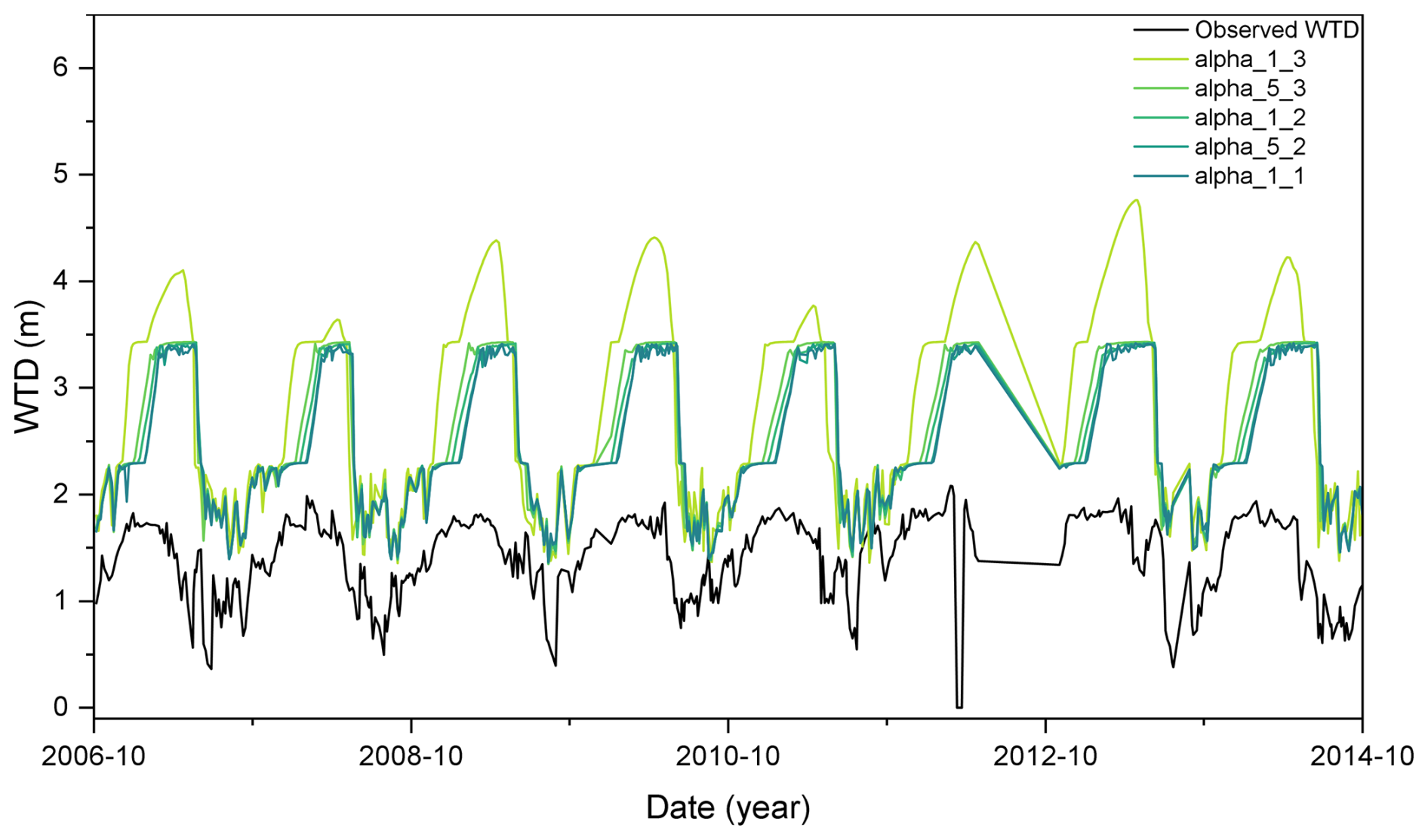
Figure 25 Sensitivity of simulated WTD to the van Genuchten parameter α with all other parameters held at their default values. The legend labels in the format “alpha_X_Y” denote α values of $X\times {\mathrm{10}}^{-Y}$ (specifically: $\mathrm{1}\times {\mathrm{10}}^{-\mathrm{3}}$, $\mathrm{5}\times {\mathrm{10}}^{-\mathrm{3}}$, $\mathrm{1}\times {\mathrm{10}}^{-\mathrm{2}}$, $\mathrm{5}\times {\mathrm{10}}^{-\mathrm{2}}$, $\mathrm{1}\times {\mathrm{10}}^{-\mathrm{1}}$).

Regarding the relationship between α and WTD, α is a scale parameter inversely related to the mean pore size (Maina and Siirila-Woodburn, 2020). Thus, lower α values indicate a greater capacity of the medium to retain water, resulting in relatively higher evapotranspiration and a deeper WTD, particularly in forested regions with high potential evapotranspiration. In addition, as the WTD deepens, the importance of α increases. This is because, with a thicker unsaturated zone, ET is primarily controlled by soil moisture and atmospheric conditions, making it more sensitive to soil hydraulic parameters in the unsaturated zone. As for the relationship between α and WTD variability, α is also the inverse of the air-entry value (Peters and Durner, 2006). A smaller α implies a higher air-entry value, allowing water to more easily fill pore spaces and increasing hydraulic conductivity, which accelerates downward water movement and leads to stronger WTD fluctuations (Corona and Ge, 2022). Conversely, larger α values imply smaller air-entry values, meaning that water has more difficulty entering pore spaces relative to air, thereby reducing unsaturated hydraulic conductivity. Lower conductivity results in slower and more delayed downward flow toward the water table. Over time, this attenuated percolation leads to a slightly lagged groundwater response and smoother WTD variations.

Comparing the effects of different parameters on WTD, changes in subsurface runoff parameters r_sub,max and f_drai can substantially alter the depth of WTD, bringing it closer to observations. In contrast, α played a more prominent role in shaping the fluctuation and lag characteristics of WTD. This suggested a practical calibration strategy in which subsurface runoff parameters are first adjusted to maintain WTD at a reasonable depth, followed by fine-tuning of other sensitive parameters to improve the temporal dynamics and variability of WTD.

4.3 Robustness of qualitative sensitivity analysis

Because qualitative sensitivity analysis involves stochastic sampling, additional experiments using two independent random seeds were conducted to evaluate the robustness of the identified sensitive parameters. Together with the original realization, three repeated experiments were available. The original experiment presented in the manuscript was designated as Seed 3 (s3), while the two newly generated realizations were designated as Seed 1 (s1) and Seed 2 (s2). For all realizations, failed simulations caused by model non-convergence were excluded before calculating sensitivity indices. Then, the screening procedure mentioned in Sect. 3.1 was applied to the additional two experiments. The robustness was evaluated using selection frequency and the mean sensitivity index among repeated realizations.

Table 7 Parameter selection results under different random seed experiments.

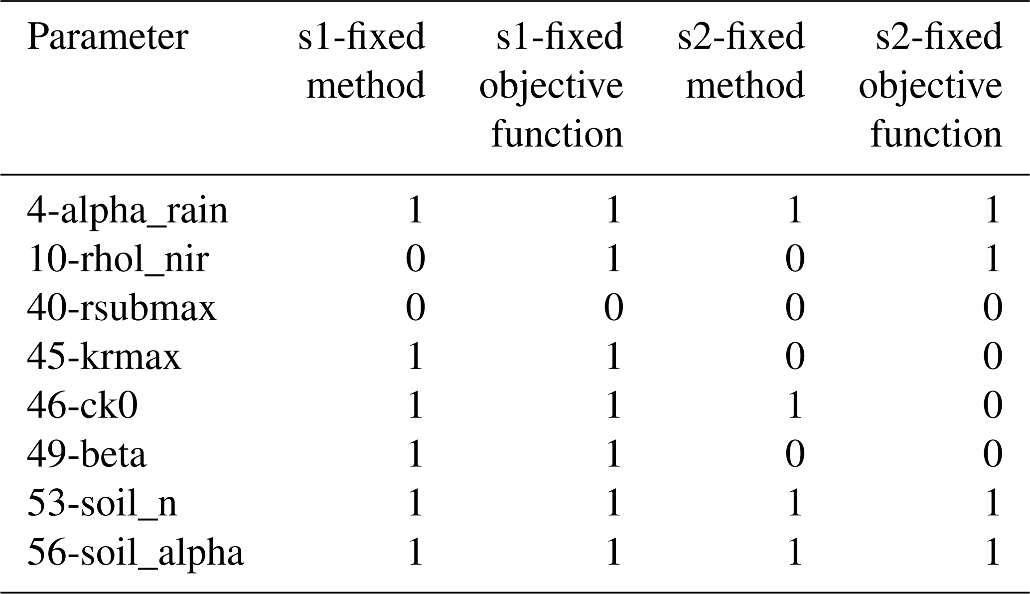
The screening results of the additional random seed experiments are shown in Table 7. In this table, 1 indicates that a parameter was selected as a sensitive parameter in the corresponding experiment, whereas 0 indicates that it was not selected. The detailed screening results are provided in Sect. S6. Overall, the repeated experiments showed that the qualitative sensitivity rankings were highly consistent for the dominant parameters but exhibited moderate variability. Among all parameters, 56-soil_alpha was identified as the most sensitive parameter in every repeated experiment and exhibited the highest selection frequency, indicating excellent robustness (Fig. 26). Similarly, parameters (i.e. 53-soil_n, 45-krmax, 49-beta, 46-ck0, 10-rhol_nir, and 4-alpha_rain) were repeatedly selected as sensitive across different random seeds (Table 7), although their detailed rankings varied. In contrast, parameter 40-rsubmax showed relatively larger variability among repeated realizations. Although it was identified as highly sensitive in the original experiment and exhibited important effects on WTD dynamics, its selection frequency decreased in additional realizations (Table 7). This suggested that the sensitivity of 40-rsubmax may be more dependent on the specific sampling trajectories compared with the dominant parameters such as 56-soil_alpha.

These results also highlight a potential limitation of qualitative sensitivity screening itself. Different screening methods characterize input-output relationships in different ways and may produce different sensitivity classifications to the same parameter, including cases where a parameter is classified as sensitive by one method but insensitive by another, or conversely. For MARS and SOT, the resulting importance measures may not represent the isolated contribution of a parameter, which can complicate the attribution of sensitivity to individual parameters and contribute to differences among screening methods (Gan et al., 2014). By contrast, MOAT changes one parameter at a time while keeping the other parameters unchanged, which may reduce such attribution ambiguity. Therefore, the use of multiple screening methods and random seeds provides an important means of cross-checking their robustness.

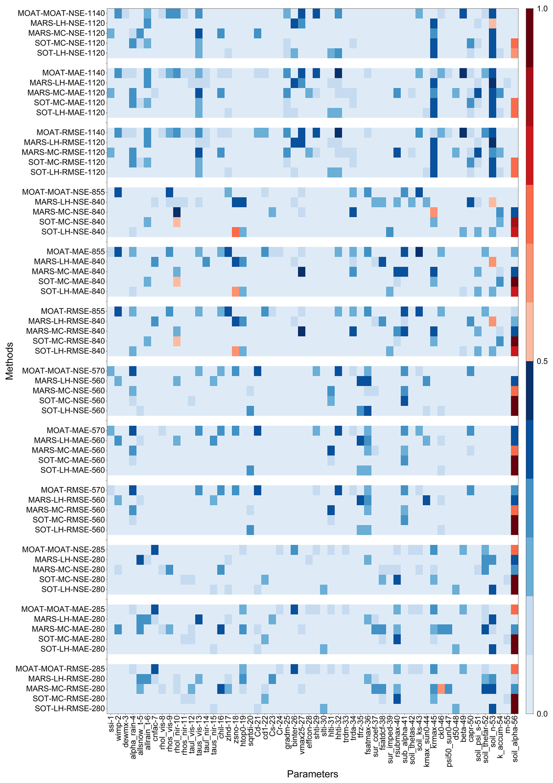
Figure 26 Mean normalized qualitative sensitivity analysis results across three independent random seed realizations (s1–s3). The normalized sensitivity index ranges from 0 to 1, where 1 and 0 represent the most and least sensitive parameters, respectively. The horizontal axis denotes parameter indices, while the vertical axis represents different analysis methods and sampling techniques, following the format “sensitivity analysis method–sampling method–objective function–sample size”.

4.4 Performance and limitations of parameter optimization for WTD simulation

Considering the cost of computation, a fixed optimization cost (about 500–1000 runs) was adopted for the evaluation. Such comparisons of fixed costs have also been conducted in previous studies (Kavetski et al., 2018), and they are divided into two types of computational budgets. The evaluations ranging from 200 to 500 times are classified as the “tight” type, while those ranging from 1000 to 5000 times are classified as the “large” type (Qin et al., 2022). The convergence behaviours of different methods are different. Some methods can still find satisfactory solutions even when the budget is limited. However, for some methods, even in the case of a large budget, there is still a significant variability in the convergence behaviour. This might be related to the complexity of the model, especially when dealing with highly parameterized models, and the speed of convergence also depends on various factors such as the sampling strategy of the algorithm (Qin et al., 2022). In addition, the optimization process was also controlled by the convergence criteria. The detailed stopping criteria of PSO, SCE, and BOBYQA implemented in PSUADE are provided in Sect. S7. The primary purpose of the optimization experiments in this study was not to benchmark the absolute global optimization capability of different algorithms, but rather to evaluate whether the sensitive parameters identified from the sensitivity-analysis framework could effectively improve WTD simulations. Therefore, a moderate computational budget in this study was considered appropriate for assessing the effectiveness of the selected parameters. Nevertheless, the use of fixed-cost evaluation for parameter optimization still has limitations. Specifically, performance metrics can be subject to sampling error under the low number of algorithm invocations (Qin et al., 2022). In addition, the relative performance may vary under larger evaluation budgets (Zhang et al., 2009). Thus, the comparison of the three optimization methods should be interpreted in the context of their practical but unequal computational budgets used in this study. Further experiments with matched evaluation budgets would be useful for a more rigorous comparison of their performance.

Although the SCE-optimized simulation substantially improved the overall WTD performance, Fig. 16 showed that the two groundwater fluctuation events between May and July 2007 were not fully reproduced. To further evaluate whether the selection of the objective function influences the performance, the existing SCE simulations were additionally assessed using Kling-Gupta efficiency (KGE, Eq. S50 in the Supplement) and event-based RMSE metrics (Sect. S8.1). The results demonstrated that the parameter set achieving the lowest global RMSE was not necessarily optimal for reproducing temporal variability (Fig. S21a). Specifically, the solution with the maximum KGE achieved a higher KGE value (0.529) than the minimum RMSE solution (0.435), while its RMSE increased by only 0.123 m compared with the global minimum RMSE solution. This indicated that optimization based solely on global RMSE may reduce overall errors while compromising event-scale dynamics. Besides the influence of objective functions, meteorological forcing uncertainty (Sect. S8.2) and freeze–thaw representation (Sect. S8.3) may also contribute to difficulties in reproducing rapid groundwater fluctuations. In addition, previous studies have shown that simplified groundwater parameterization schemes may limit the ability of land surface models to represent groundwater recharge dynamics, particularly during intense precipitation events (Sobaga et al., 2023). Furthermore, uncertainties associated with groundwater observations may also introduce deviations. Overall, accurately reproducing event-scale groundwater fluctuations requires further improvements in groundwater process parameterization and the integration of multi-objective optimization approaches in future studies.

5 Conclusions

In this study, a CoLM-PSUADE coupling framework was developed to integrate parameter sensitivity diagnosis, dimensionality reduction, and parameter optimization within a unified workflow for groundwater-related modeling. Using in-situ water table depth (WTD) observations at the GGF mountain forest site, the framework provided a systematic approach to identify influential parameters and reduce the dimensionality of the calibration problem under the studied site conditions.

The initial qualitative sensitivity analyses identified eight stably sensitive parameters (56-soil_alpha, 45-krmax, 4-alpha_rain, 53-soil_n, 49-beta, 10-rhol_nir, 46-ck0, and 40-rsubmax) governing soil water movement, subsurface runoff, plant hydraulics, and surface infiltration processes. Subsequent RSMSobol-based quantitative analysis provided a complementary assessment of these eight parameters and identified a core group (56-soil_alpha, 53-soil_n, 49-beta, 45-krmax, 40-rsubmax, and 4-alpha_rain). Building on this reduced parameter space, parameter optimization using SCE, PSO, and BOBYQA demonstrated that targeted calibration can substantially improve WTD simulation performance, with SCE identifying the lowest-RMSE solution most rapidly. To further assess the robustness of the initial qualitative sensitivity results, two additional experiments using independent random seeds were conducted. These experiments demonstrated that qualitative sensitivity rankings were generally consistent for the dominant parameters but exhibited variability among different random-seed realizations. In particular, 40-rsubmax was identified in the initial screening but was not selected as sensitive in the summarized screening results of either additional random-seed realization. In contrast, 56-soil_alpha maintained its top sensitivity ranking across all experiments, confirming its robust and dominant influence on WTD simulations.

Among identified sensitive parameters, the subsurface runoff parameter r_sub,max was unique in exhibiting a clear inflection point in the parameter-RMSE relationship, and the soil hydraulic parameter α was identified as the most sensitive parameter. From a mechanistic perspective, subsurface runoff parameters (r_sub,max and f_drai) primarily control the mean state of WTD by regulating runoff generation and decay, while the soil hydraulic parameter α governs soil water retention and vertical transport processes, thereby controlling variability and temporal response. Based on these results, a stepwise calibration strategy was recommended, prioritizing subsurface runoff parameters to constrain mean WTD, followed by other sensitive parameters to improve temporal dynamics.

It should be noted that although the GGF site selected in this study is representative for studying interactions between WTD dynamics and key hydrological processes such as runoff, infiltration, evaporation, and freeze–thaw, several limitations remain. The sensitivity results obtained in this study are specific to the GGF mountain forest site and reflect the combined effects of its hydroclimatic conditions, soil properties, vegetation characteristics, and groundwater regime. Single-point simulations cannot fully capture the spatial heterogeneity of parameter sensitivities under different climate conditions and land-surface characteristics. In addition, the relatively short sensitivity-analysis period may limit the assessment of temporal variations in parameter sensitivities under different hydrological conditions. Although repeated random seed experiments improved the assessment of sampling uncertainty, variations in sensitivity rankings indicate that qualitative sensitivity analysis remain partly dependent on sampling trajectories. Moreover, considering WTD as a single target variable may lead to parameter equivalence. This issue is exacerbated by the limited availability of observational data, resulting in insufficiently constrained parameter uncertainty. Nevertheless, the proposed research framework provides a systematic approach for sensitivity analysis and sensitivity-guided parameter optimization, offering a foundation for broader applications in groundwater-related land surface modeling. Future studies should extend the framework to multi-site and regional-scale applications. Incorporating longer simulation periods and multi-variable observations will further improve parameter identifiability.

Appendix A: Principles and formulations of sensitivity analysis methods

A1 MOAT method

MOAT is a gradient-based sensitivity analysis method. The sensitivity of model performance to an input parameter is quantified by elementary effects, which approximate local partial derivatives with respect to the parameter (Guerrero et al., 2017). The modified mean and standard deviation of these elementary effects represent overall effects and interaction effects of input parameters, respectively. Larger values of the modified mean indicate stronger parameter sensitivity, while larger values of the standard deviation suggest more significant interactions with other input parameters (Li et al., 2013). Because MOAT makes no assumptions about the relationships between model parameters and model performance, it is considered a robust screening method (Guerrero et al., 2017). The main equations are given as follows (Gan et al., 2014).

First, the range of each input parameter is normalized to [0,1]. Each parameter may take on values from:

$$\begin{array}{}\text{(A1)}& X=\left\{\mathrm{0},{\displaystyle \frac{\mathrm{1}}{p-\mathrm{1}}},\mathrm{\dots },\mathrm{1}\right\},\end{array}$$

where X is the set of discretized levels of the input parameter, p is the number of levels into which the parameter space is divided.

For each input parameter, the elementary effect is calculated as an approximation of the first-order derivative. This metric quantifies the variation in model output caused by a change in a single parameter while all other input parameters are fixed:

$$\begin{array}{}\text{(A2)}& {\mathrm{\text{EE}}}_i={\displaystyle \frac{f\left(x_{\mathrm{1}},\mathrm{\dots },x_i+\mathrm{\Delta },\mathrm{\dots },x_k\right)-f\left(x_{\mathrm{1}},\mathrm{\dots },x_i,\mathrm{\dots },x_k\right)}{\mathrm{\Delta }}},\end{array}$$

where EE_i is the elementary effect of the ith parameter, Δ is a predetermined multiple of $\frac{\mathrm{1}}{p-\mathrm{1}}$, x is the parameter, and k is the number of parameters.

To ensure statistical robustness, each input parameter is sampled r times, which is equals tor different paths. Elementary effects EE_i are calculated for each x_i along each path, from which the sensitivity indices are derived as follows:

$$\begin{array}{}\text{(A3)}& {\displaystyle }{\mathit{\mu }}_i^{*}={\displaystyle \frac{\mathrm{1}}{r}}\sum _{j=\mathrm{1}}^r\left|{\text{EE}}_i^{\left(j\right)}\right|,\text{(A4)}& {\displaystyle }{\mathit{\sigma }}_i^{*}=\sqrt{{\displaystyle \frac{\mathrm{1}}{r-\mathrm{1}}}\sum _{j=\mathrm{1}}^r{\left(\left|{\text{EE}}_i^{\left(j\right)}\right|-{\mathit{\mu }}_i^{*}\right)}^{\mathrm{2}}},\end{array}$$

where ${\mathit{\mu }}_i^{*}$ is modified mean of EE_i, and ${\mathit{\sigma }}_i^{*}$ is modified standard deviation. The r−1 is used for ${\mathit{\sigma }}_i^{*}$, consistent with the implementation.

A2 MARS method

MARS is a regression model that extends linear modeling by automatically incorporating piecewise linear basis functions to capture nonlinearities and variable interactions in high-dimensional data. The relative importance of input parameters is evaluated by re-assessing model performance after removing each parameter from the regression function (Guerrero et al., 2017). A larger reduction in the model performance indicates a higher importance of the corresponding parameter. However, this approach is less robust because it assumes a fixed functional relationship between model performance and input parameters (Guerrero et al., 2017). The regression function is composed of a series of basic functions and can be expressed as follows (Gan et al., 2014):

$$\begin{array}{}\text{(A5)}& Y=a_{\mathrm{0}}+\sum _{m=\mathrm{1}}^M{a}_m\prod _{k=\mathrm{1}}^{K_m}{\left[s_{km}\left(x_{v\left(k,m\right)}-t_{km}\right)\right]}_{+},\end{array}$$

where a₀ is a constant term, a_m denotes the fitting coefficient of the mth basis function, M is the total number of basic functions, K_m is the number of knots, s_km takes values of 1 or −1 and represents the right or left sense of step function, v(k,m) is the label of independent value, and t_km is the knot location.

MARS first constructs an overfitted model by subsequently adding all input parameters. The model is then modified by removing one parameter at a time to generate a series of modified models. Both the overfitted and the modified models are used to calculate the generalized cross validation (GCV) index:

$$\begin{array}{}\text{(A6)}& {\displaystyle }\text{GCV}\left(M\right)={\displaystyle \frac{\mathrm{1}}{N}}{\displaystyle \frac{\sum _{k=\mathrm{1}}^N{\left(Y_k-\widehat{Y_k}\right)}^{\mathrm{2}}}{{\left[\mathrm{1}-\frac{C\left(M\right)}{N}\right]}^{\mathrm{2}}}},\text{(A7)}& {\displaystyle }C\left(M\right)=\mathrm{1}+c\left(M\right)d,\end{array}$$

where M is the model, N is the number of observations, Y_k is the kth observation, $\widehat{Y_k}$ is the estimated value of Y_k, C(M) is the number of effective parameters, d is the effective degrees of freedom, and c(M) is a penalty term associated with adding a basis function.

The increase in the GCV value between the modified and the overfitted model is considered as the importance index for the removed parameter. A larger increase in GCV suggests a higher importance of that parameter. Accordingly, the sensitivity score of the ith parameter is defined as:

$$\begin{array}{}\text{(A8)}& \text{score}\left(i\right)={\displaystyle \frac{\mathrm{\Delta }g\left(i\right)}{max\left\{\mathrm{\Delta }g\left(\mathrm{1}\right),\mathrm{\Delta }g\left(\mathrm{2}\right),\mathrm{\dots },\mathrm{\Delta }g\left(n\right)\right\}}}\times \mathrm{100},\end{array}$$

where Δg(i) indicates the increase in the GCV value resulting from the removal of the ith parameter.

A3 SOT method

The SOT method is a tree-based method. It represents model performance as the sum of multiple binary decision trees constructed from model parameters. However, it is less robust, as this approach hinges on the assumption that the relationship between input parameters and model performance can be captured by such a tree structure (Guerrero et al., 2017). Each parameter splits the parameter space into two regions with distinct responses. Overall model performance is then obtained by aggregating the simulated results across all partitioned regions. The relative importance of a parameter is measured by the total number of splits associated with that parameter, with parameters appearing in more splits regarded as more important (Li et al., 2013).

The structure of a single tree consists of decision nodes and terminal nodes (Chipman et al., 2010). Each decision node partitions the input parameter space $X=\left\{x_{\mathrm{1}},\mathrm{\dots },x_p\right\}$ according to a splitting rule. Through a sequence of decisions from the root node to a leaf node, each input parameter is assigned to a terminal node associated with a prediction value ${\mathit{\mu }}_i\in M=\left\{{\mathit{\mu }}_{\mathrm{1}},{\mathit{\mu }}_{\mathrm{2}},\mathrm{\dots },{\mathit{\mu }}_b\right\}$. The SOT method is then defined as:

$$\begin{array}{}\text{(A9)}& Y=\sum _{j=\mathrm{1}}^{m}g\left(X;T_j,M_j\right)+\mathit{ϵ},\end{array}$$

where T_j is the jth binary decision tree, M_j is the set of terminal node parameters, $g\left(X;T_j,M_j\right)$ is the function which assigns μ_i to X, m is the total number of trees, ϵ is a random noise term with $\mathit{ϵ}\sim \mathcal{N}\left(\mathrm{0},{\mathit{\sigma }}^{\mathrm{2}}\right)$.

In the above splitting procedure, the residual sum of squares (RSS) is used as the splitting criterion. The parameter that produces the largest reduction in RSS is selected to split the node until each terminal node includes minimum number of data points (Gan et al., 2014). Subsequently, the total number of splits associated with each parameter is considered as a score metric (Gan et al., 2014). A larger number of splits indicates higher sensitivity of the corresponding input parameter. The score of the ith input parameter is defined as:

$$\begin{array}{}\text{(A10)}& \text{score}\left(i\right)={\displaystyle \frac{p\left(i\right)}{max\left\{p\left(\mathrm{1}\right),p\left(\mathrm{2}\right),\mathrm{\dots },p\left(n\right)\right\}}}\times \mathrm{100},\end{array}$$

where p(i) denotes the number of splits associated with the ith input parameter.

A4 Sobol method

The Sobol method is a variance-based method. It quantifies parameter sensitivity by decomposing the total variance into contributions from individual input parameters and their interactions (Li et al., 2013). This method assumes that the model output can be decomposed into terms of increasing dimensionality:

$$\begin{array}{}\text{(A11)}& \begin{array}{rl}f\left(X\right)& =f_{\mathrm{0}}+\sum _{i=\mathrm{1}}^n{f}_i\left(x_i\right)+\sum _{\mathrm{1}\le i<j\le n}{f}_{ij}\left(x_i,x_j\right)+\mathrm{\cdots }\\ & +f_{\mathrm{1},\mathrm{2},\mathrm{\cdots },n}\left(x_{\mathrm{1}},x_{\mathrm{2}},\mathrm{\cdots },x_n\right),\end{array}\end{array}$$

where $Y=f\left(X\right)=f\left(x_{\mathrm{1}},x_{\mathrm{2}},\mathrm{\dots },x_n\right)$ is the model output, x_i∈[0,1], and f₀ is the constant term.

Accordingly, the total variance of the model output can be decomposed as:

$$\begin{array}{}\text{(A12)}& V=\sum _{i=\mathrm{1}}^n{V}_i+\sum _{\mathrm{1}\le i<j\le n}{V}_{ij}+\mathrm{\cdots }+V_{\mathrm{1},\mathrm{2},\mathrm{\cdots },n},\end{array}$$

where V is the total variance, V_i denotes the main effect variance associated with x_i, V_ij denotes the interaction variance between x_i and x_j, and $V_{\mathrm{1},\mathrm{2},\mathrm{\cdots },n}$ is the variance due to interactions among all input factors.

By dividing each variance component by total variance V, the normalized Sobol sensitivity indices are quantified as:

$$\begin{array}{}\text{(A13)}& \sum _{i=\mathrm{1}}^n{S}_i+\sum _{\mathrm{1}\le i<j\le n}{S}_{ij}+\mathrm{\cdots }+S_{\mathrm{1},\mathrm{2},\mathrm{\cdots },n}=\mathrm{1},\end{array}$$

where $S_i=V_i/V$ is the first-order Sobol sensitivity index of x_i and represents its main effect. $S_{ij}=V_{ij}/V$ is the second-order Sobol index, accounting for the interaction effect between x_i and x_j.

The total effect sensitivity index of parameter x_i is defined as:

$$\begin{array}{}\text{(A14)}& S_{T_i}=\sum S_{\left(i\right)},\end{array}$$

where S_(i) is the sensitivity of x_i, (i) denotes all subsets of indices containing i.

To facilitate comparison of the results across different experiments, the concepts of relative importance and cumulative importance were introduced. The relative importance of the ith parameter in parameter set A is defined as:

$$\begin{array}{}\text{(A15)}& C\left(i\right)={\displaystyle \frac{S_{T_i}}{\sum _{k=\mathrm{1}}^n{S}_{T_k}}},\end{array}$$

where C(i) denotes the relative importance of parameter i within set A; n is the total number of parameters in set A; and $S_{T_i}$ represents the Sobol' total-order index of parameter i. The cumulative importance of a parameter set is then defined as the sum of the relative importance values.

A5 Min–max Normalization

To enable a consistent comparison of parameter screening results across different qualitative sensitivity analysis methods, the sensitivity metrics derived from the MOAT, MARS, and SOT methods are scaled using min-max normalization. The original sensitivity metrics are linearly mapped into the range [0, 1] using the following function:

$$\begin{array}{}\text{(A16)}& X^{*}={\displaystyle \frac{X-X_{\min }}{X_{\max }-X_{\min }}},\end{array}$$

where X^* is the normalized sensitivity index, X is the original sensitivity metric, and X_min and X_max represent the minimum and maximum values of the metrics within each method, respectively.

A6 Response surface validation metrics

After loading the parameter inputs and objective function outputs into PSUADE, the quality of the response surface trained on these samples can be evaluated. A comprehensive assessment is performed based on cross-validation errors and the goodness of fit. Assuming the true output (i.e. the corresponding PSUADE output metric) is y and the predicted output from the response surface is $\widehat{y}$, the evaluation metrics are defined as follows:

$$\begin{array}{}\text{(A17)}& {\displaystyle }{\text{err}}_{\mathrm{avgs}}={\displaystyle \frac{\mathrm{1}}{n}}\sum _{i=\mathrm{1}}^n{\displaystyle \frac{{\widehat{y}}_i-y_i}{\left|y_i\right|}},\text{(A18)}& {\displaystyle }{\text{err}}_{\mathrm{rmss}}=\sqrt{{\displaystyle \frac{\mathrm{1}}{n}}\sum _{i=\mathrm{1}}^n{\left({\displaystyle \frac{\left|{\widehat{y}}_i-y_i\right|}{\left|y_i\right|}}\right)}^{\mathrm{2}}},\text{(A19)}& {\displaystyle }{\text{err}}_{\mathrm{maxs}}=\underset{\mathrm{1}\le i\le n}{\max }\left({\displaystyle \frac{\left|{\widehat{y}}_i-y_i\right|}{\left|y_i\right|}}\right),\text{(A20)}& {\displaystyle }{\text{err}}_{\mathrm{maxs},\mathrm{base}}=\left|y_{i^{*}}\right|,i^{*}=\underset{\mathrm{1}\le i\le n}{\mathrm{argmax}\left({\widehat{y}}_i-y_i\right)},\text{(A21)}& {\displaystyle }{\text{err}}_{\mathrm{maxs}\mathrm{2}}=\underset{\mathrm{1}\le i\le n}{\max }\left({\displaystyle \frac{\left|{\widehat{y}}_i-y_i\right|}{y_{\max }-y_{\min }}}\right),\text{(A22)}& {\displaystyle }{R}_{\mathrm{rsm}}^{\mathrm{2}}=\mathrm{1}-{\displaystyle \frac{\sum _{i=\mathrm{1}}^n{\left({\widehat{y}}_i-y_i\right)}^{\mathrm{2}}}{\sum _{i=\mathrm{1}}^n{\left(y_i-\stackrel{\mathrm{‾}}{y_i}\right)}^{\mathrm{2}}}},\end{array}$$

where n is the total number of samples, y_i and ${\widehat{y}}_i$ are the true and predicted values of the ith sample, err_avgs is the scaled mean error, err_rmss is the scaled root mean square error, err_maxs is the scaled maximum error, err_maxs,base is the absolute true value of the sample corresponding to the scaled maximum error, err_maxs2 is the maximum scaled error based on the output range, and $R_{\mathrm{rsm}}^{\mathrm{2}}$ is the coefficient of determination, indicating the goodness of fit of the response surface in approximating the original input-output relationship.

For cross-validation, the number of groups K is set to 20 (as recommended by the PSUADE manual). The training set for the xth group consists of samples outside the interval [$x\cdot \frac{n}{K},\left(x+\mathrm{1}\right)\cdot \frac{n}{K}$], while the validation set comprises the samples within this interval. The final error metrics are not simple averages of the individual groups. Instead, the overall evaluation metrics are calculated as follows:

$$\begin{array}{}\text{(A23)}& {\displaystyle }{\text{Err}}_{\mathrm{avgs}}={\displaystyle \frac{\mathrm{1}}{N}}\sum _{j=\mathrm{1}}^K\sum _{i\in G_j}\left({\displaystyle \frac{{\widehat{y}}_i-y_i}{\left|y_i\right|}}\right),\text{(A24)}& {\displaystyle }{\text{Err}}_{\mathrm{rmss}}=\sqrt{{\displaystyle \frac{\mathrm{1}}{N}}\sum _{j=\mathrm{1}}^K\sum _{i\in G_j}{\left({\displaystyle \frac{\left|{\widehat{y}}_i-y_i\right|}{\left|y_i\right|}}\right)}^{\mathrm{2}}},\text{(A25)}& {\displaystyle }{\text{Err}}_{\mathrm{maxs}}=\underset{\mathrm{1}\le j\le K}{\max }\left({\text{err}}_{\mathrm{maxs},j}\right),\text{(A26)}& {\displaystyle }{\text{Err}}_{\mathrm{maxsb}}=\underset{\mathrm{1}\le j\le K}{\max }\left({\text{err}}_{\mathrm{maxs},\mathrm{base},j}\right),\text{(A27)}& {\displaystyle }{\text{Err}}_{\mathrm{maxs}\mathrm{2}}=\underset{\mathrm{1}\le j\le K}{\max }\left({\text{err}}_{\mathrm{maxs}\mathrm{2}}\right),\end{array}$$

where N is the total number of samples, K is the number of groups, and G_j represents the set of samples in the jth group.

If Err_rmss deviates significantly from 0, it indicates the presence of systematic bias. If Err_maxs is greater than 1 and Err_maxsb is non-negative, it suggests a relatively significant fitting error. However, if this error value is large while the variation range of y_i is also substantial, further analysis in conjunction with the magnitude of Err_maxs2 is required. In such cases, a smaller Err_maxs2 is considered acceptable. Theoretically, the predicted and actual values in cross-validation should align along the 1:1 diagonal line, and the overall fitting performance can be judged by combining this visual assessment with the $R_{\mathrm{rsm}}^{\mathrm{2}}$.

Appendix B: Principles of parameter optimization methods

B1 SCE method

The SCE method is a global optimization algorithm developed by Duan et al. (1994, 1992, 1993), which is widely utilized for calibrating large-scale watershed models. This method integrates the advantages of competitive biological evolution, deterministic search, and random search, thereby reducing parameter uncertainty and accelerating the search for the global optimum. Its core idea involves complex shuffling and the systematic evolution of a “complex” of points spanning the parameter space. During the shuffling step, the initial population is randomly partitioned into several complexes. Within each complex, points are evolved through competitive mechanisms to generate new populations. This process enhances diversity in the search space and prevents the algorithm from being trapped in local optima. The evolution step employs selection, crossover, and mutation operations iteratively to update the points in each complex until a solution satisfying the stopping criterion is achieved.

B2 PSO method

The PSO method is a global optimization algorithm developed by Kennedy and Eberhart (Kennedy and Eberhart, 1995). As a heuristic optimization technique rooted in collective intelligence, it is inspired by the social foraging behaviour of bird flocks. Compared to adaptive random search algorithms, PSO utilizes a set of potential solutions, commonly known as a population, to achieve global or near-global optima through mechanisms of collaboration and competition (Gill et al., 2006). Within this framework, each potential solution is abstracted as a particle moving through the search space. The position of particle represents a candidate solution, while its velocity determines the search direction and rate. To balance global search and local optimization, particles iteratively adjust their velocity and position guided by both their individual historical optima and the collective historical optima.

B3 BOBYQA method

The BOBYQA method is a derivative-free algorithm developed by Powell solving bound-constrained optimization problems (Powell, 2009). The core principle of this algorithm is to construct a quadratic model that approximates the objective function near the current search point. Rather than seeking the global optimum directly, BOBYQA explores a trust region, defined as a neighbourhood focused on the current point with a predefined radius, to determine a descent step based on the local quadratic model. When generating candidate points, BOBYQA ensures that both the search direction and step length do not violate the parameter boundaries. If a predicted optimum lies outside these limits, the algorithm projects it back onto the feasible domain. As a derivative-free method, BOBYQA functions as a “black-box” optimizer and does not require gradient information from the objective function.