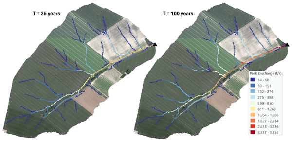
High-resolution mapping of pluvial flooding in ungauged agricultural catchments

Accurate pluvial flood mapping in ungauged agricultural catchments is often constrained by a lack of calibration data. This study evaluates a parsimonious, high-resolution (1 m) distributed framework assessing peak discharge along concentrated flow paths, validated against 39 events recorded at two nested outlets (84 and 111 ha) of a single experimental catchment. The framework decouples the rainfall-runoff process to systematically compare adjusted Soil Conservation Service Curve Number (SCS-CN) formulations against two spatially explicit routing algorithms (SCS velocity method vs. Simulator for Water Resources in Rural Basins, SWRRB). Within this specific local context, findings demonstrate that the Jain initial abstraction method significantly reduces volumetric bias, with the distributed approach statistically outperforming lumped modelling. However, performance remains strictly regime-dependent, driven by rainfall intensity rather than total depth. This exposes the structural limits of static Curve Number (CN) parameterizations in capturing rapid Hortonian dynamics, causing the model to dampen minor events while amplifying high-intensity storms. Regarding hydraulic transfer, both routing strategies yield statistically equivalent performance (median Kling-Gupta Efficiency (KGE) values of 0.35 vs. 0.34). Crucially, while the routing phase acts as a mechanical propagator of volumetric uncertainty, it effectively synchronizes the overall runoff window. Applied to 25- and 100-year design storms, this framework illustrates hydrodynamic attenuation and kinematic synchronization at confluences. While primarily validated on a single well-monitored catchment, these findings illustrate the approach's potential to pinpoint hydraulic hotspots, with initial benchmarks indicating promising scalability to larger agricultural landscapes.

1 Introduction

Recognized as a major hydrological hazard, pluvial flooding occurs when intense rainfall generates excessive surface runoff and rapid, localized water accumulation, distinguishing it from traditional riverine flooding. Pluvial flood exposure across Europe is immense; in England alone, roughly one million properties are at high risk of surface water flooding, triple the number exposed to traditional riverine and coastal hazards (Environment Agency, 2025). Intensified by climate change, these rapid pluvial floods constitute a growing natural threat. The devastating July 2021 floods in Western Europe starkly illustrate this amplification of extreme meteorological events. Within just three days (14–16 July), parts of the Belgian Vesdre basin received up to 290 mm of rain (Journée et al., 2023), representing nearly one-fifth of the regional annual average (Erpicum et al., 2018). Predicting such localized hazards remains a fundamental hydrological challenge, a difficulty further compounded by a lack of reliable monitoring in small or agricultural catchments, where gauge data are typically absent (Blöschl et al., 2019). Furthermore, while remote sensing (e.g., Copernicus EMS) provides useful a posteriori validation of flooded areas (Munawar et al., 2022), proactive risk management requires comprehensive a priori hazard mapping across all potentially vulnerable sites, regardless of past events. While the European Floods Directive (2007/60/EC) mandates a precise quantification of these risks, meeting this requirement remains a critical challenge in ungauged catchments, where discharge data are non-existent. Consequently, there is an urgent need to develop robust, parsimonious modelling tools capable of spatially estimating and quantifying pluvial flood risks in unmonitored agricultural landscapes.

To address the complexities of pluvial flood risk mapping, the scientific community has developed a spectrum of methodological approaches specifically tailored to surface runoff. In data-scarce agricultural catchments, alternative index-based approaches have gained prominence; for instance, Kazakis et al. (2015), Kourgialas and Karatzas (2011), and Vojtek et al. (2019) developed multi-criteria susceptibility indices integrating static factors such as topography, land use, and geology. While operationally efficient for identifying potential hazard zones (Mudashiru et al., 2021), these heuristic methods remain essentially qualitative, ranking susceptibility without quantifying dynamic flow magnitudes. Consequently, they overlook the non-linear temporal dynamics of intense rainfall events and the specific connectivity of hillslope rills (Papaioannou et al., 2018). To overcome these limitations, recent literature increasingly advocates rain-on-grid approaches (e.g., Ennouini et al., 2024; Macchione et al., 2026; Michailidi et al., 2018). Unlike static indices, these approaches simulate spatially resolved runoff responses, enabling the generation of hazard maps founded on quantitative values rather than qualitative proxies.

However, operationalizing these distributed models to address the specific challenge of Prediction in Ungauged Basins (PUB) requires tools that strike a balance between physical representativeness and parsimony (Hrachowitz et al., 2013). In this context, the Hidropixel model has emerged as a promising tool (Costa et al., 2019; Veeck et al., 2020). In contrast to lumped models that average parameters over an entire basin, Hidropixel utilizes a fully distributed architecture where each grid cell functions as an independent micro-catchment. The model operates in a two-step process. First, it calculates the effective rainfall volume locally for every pixel using the Soil Conservation Service Curve Number (SCS-CN) method, based on soil type, land use, and antecedent moisture conditions (Mishra et al., 2004; Mishra and Singh, 2003; Sahu et al., 2012). This local excess is then transformed into a pixel-specific hydrograph and routed to the catchment outlet (Sect. 2.3). Most recently, Lima et al. (2024) upgraded the framework to the TUH+ version (Triangular Unit Hydrograph with lag parameter). This formulation refines the standard convolution process by integrating a time-lag parameter (T_v), which explicitly accounts for the translation and storage effects inherent in runoff routing. By spatially varying the unit hydrograph (UH) parameters for every pixel, the TUH+ approach significantly enhances the simulation of hydrograph shape, specifically peak magnitude and timing (Lima et al., 2024).

Despite the model's structural strengths, its internal components require optimization for ungauged applications. Regarding runoff generation, the SCS-CN method remains the standard due to its computational simplicity, stability, and reliance on accessible catchment data. While widely adopted (e.g., Neitsch et al., 2011; Scharffenberg and Fleming, 2013), its conventional application is still challenged by recent studies (Panigrahi and Ramadas, 2025; Soulis, 2021). One of the main criticisms concerns the initial abstraction ratio (λ), traditionally fixed at 0.2. This value is often excessive for agricultural catchments, leading to a systematic underestimation of runoff volumes for small-to-moderate rainfall events. Consequently, modern adaptations – such as those proposed by Jain et al. (2006), Verma et al. (2017), and Woodward et al. (2003) – advocate for alternative parameterizations (Sect. 2.3.1). Moreover, the method's inherent inability to explicitly account for rainfall intensity dynamics limits its physical realism during short, high-intensity storms (Grimaldi et al., 2013; Ponce and Hawkins, 1996). Therefore, implementing Hidropixel effectively requires moving beyond standard parameters to systematically test these alternative CN formulations.

A further, related source of error stems from the common practice of representing an entire heterogeneous catchment with a single, area-weighted composite CN. Because the SCS-CN equation is strictly non-linear, runoff computed from a composite CN can differ substantially – and often underestimates the total volume – compared to applying the method separately to each heterogeneous sub-area and summing the results (Grove et al., 1998). This fundamental spatial-aggregation error, and approaches to mitigate it by explicitly representing the spatial distribution of runoff-producing areas, have been extensively documented, notably in recent empirical and synthetic-data studies (Palli-Gravani et al., 2026; Soulis and Valiantzas, 2012). The distributed, pixel-scale approach adopted in this study therefore aligns with and reinforces this well-established consensus on watershed heterogeneity.

Equally critical to the flood response is the routing of this effective runoff, a process governed by the estimation of flow velocity. Traditionally, this translation is parameterized via the time of concentration (T_c), a metric fraught with epistemic uncertainty (Grimaldi et al., 2012; Michailidi et al., 2018). Empirical formulas can yield results differing by nearly one order of magnitude for the same catchment, drastically altering the resulting peak discharge (Q_p) and time to peak (T_p). To address the limitations of lumped T_c equations, there is a specific need to integrate spatially explicit routing methods that derive velocity directly from local topography and roughness, such as the SCS velocity method (USDA-NRCS, 2010) or the Simulator for Water Resources in Rural Basins (SWRRB) formulation (Williams et al., 1985). The adoption of these methods is justified by their suitability for data-scarce environments and their compatibility with high-resolution geographic information system (GIS) datasets. Coarser grid resolutions smooth topographic gradients and artificially accelerate flow concentration, compromising routing accuracy (Grimaldi et al., 2012; Veeck et al., 2020). However, these kinematic approximations are not without limitations. First, they remain sensitive to roughness parameterization (Manning's n), which is difficult to validate in ungauged channels (Arcement and Schneider, 1989). Second, and arguably more critical, is the issue of non-linearity. Standard velocity methods typically impose a stationary travel time field determined exclusively by topography and roughness. This approach disregards the hydrodynamic dependence of velocity on flow depth (Gericke and Smithers, 2014; Grimaldi et al., 2012; Walega et al., 2020), which can lead to substantial inaccuracies in hydrograph representation and an underestimation of peak discharge timing during extreme events (Michailidi et al., 2018).

In light of this context, the primary goal of this study is to develop a robust methodology for high-resolution mapping of runoff flood hazard by quantifying peak discharge distributions across ungauged catchments. To evaluate this framework, the methodology is applied to an experimental agricultural catchment, providing a high-quality dataset to validate the model's performance against observed rainfall-runoff events. Specifically, the research objectives are threefold:

• i.

  Identify the most effective runoff calculation method by comparing several SCS-CN formulations (Standard, Jain, Woodward, and Hawkins) under both lumped and fully distributed modelling approaches.

• ii.

  Determine the most accurate approach for calculating travel times by contrasting the SCS Velocity and SWRRB methods, leveraging high-resolution (1 m) topographic and land-use data.

• iii.

  Spatialize runoff flood hazard by using the optimized model to generate fine-scale spatially distributed maps of Q_p along concentrated flow paths for specific return periods.

2 Methodology

2.1 Study area

The study area is a headwater catchment located in Chastre, representative of the loess belt region of central Belgium (50°36^′23.02^′′ N, 4°35^′42.33^′′ E; Fig. 1). The Belgian loess belt is historically characterized by high rates of water-induced soil erosion and frequent pluvial, often muddy, flood events. The watershed has been extensively described and monitored in previous studies, notably by Cantreul et al. (2020) and Pineux et al. (2017), providing a robust dataset for validation, including continuous hydrological observations since 2012. The catchment exhibits a gently undulating topography typical of the region, with elevations ranging from 132 to 161 m and gentle to moderate slopes varying between 0.25 % and 17 %, with a mean slope of 3.8 %. The total catchment area (outlet = Point 3 in Fig. 1) covers 111 ha and contains a nested sub-catchment (outlet = Point 2) of 84 ha. Morphologically, the basin is elongated, with the longest hydraulic path (LHP) extending over 2036 m from the main outlet (Point 3). Hydrologically, it functions as a “dry” valley, lacking a permanent river network and governed entirely by episodic runoff dynamics.

The catchment is characterized by a temperate oceanic climate (Köppen–Geiger Cfb), with a long-term mean annual temperature of 10.3 °C and precipitation of 820 mm over the 1991–2020 reference period (IRM, 2023). Geologically, the catchment is underlain by thick Quaternary loess deposits that support Cambisols and Luvisols. These soils feature a clay-enriched B horizon which, although conducive to natural drainage, has been progressively truncated by diffuse erosion on the hillslopes. Anthropogenic pressure is significant, with 98 % of the area dedicated to arable land and negligible forest cover (0.11 %). The landscape is emblematic of intensive open-field cropping systems, dominated by large parcels (on average 14.5 ha) where semi-natural features such as hedgerows are sparse. This specific configuration – intensive cultivation combined with the high susceptibility of loess soils to structural degradation (crusting) – renders the catchment highly prone to surface sealing and the rapid concentration of runoff along concentrated flow paths.

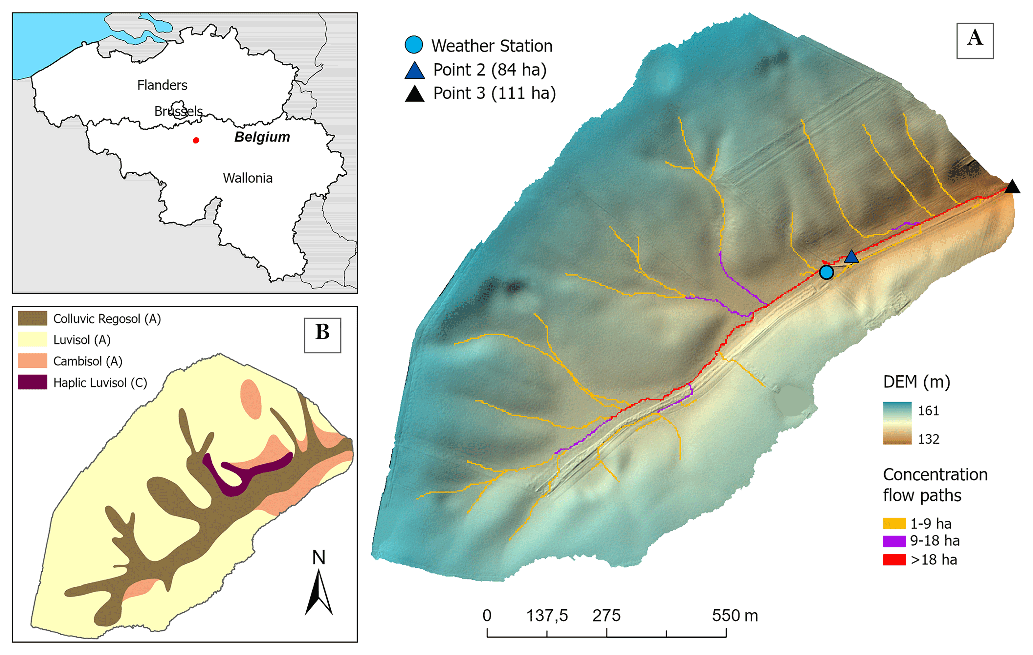
Figure 1 (A) Location of the study catchment and its two nested discharge monitoring points in Belgium. (B) Soil map classified according to the WRB reference groups. Superimposed letters denote the SCS Hydrologic Soil Groups used to parameterize runoff potential. Map data: DEM and soil map © Service public de Wallonie (https://geoportail.wallonie.be, last access: 19 October 2026).

The nested configuration of the catchment facilitates a multi-site validation strategy. This setup allows Q_p estimates to be verified at two distinct scales within the drainage network, thereby assessing the model's spatial consistency.

2.2 Methodological approach

To explore the potential of a robust framework for ungauged catchments, this study moves beyond site-specific calibration to focus on the spatial distribution of Q_p along concentrated flow paths. The proposed methodological workflow (Fig. 2) utilizes the Hidropixel model (Lima et al., 2024) at a 1 m resolution, structured around a systematic evaluation of (i) runoff generation and (ii) hydraulic transfer. This framework is tested against a dataset of 39 rainfall-runoff events from an experimental agricultural catchment. The validation follows a stepwise process: first assessing runoff volume accuracy under various initial abstraction hypotheses, then evaluating routing performance regarding peak timing and magnitude, before finally synthesizing these components into an operational tool for flood hazard mapping.

The runoff generation mechanism (Phase 1) – the conversion of raw rainfall into effective runoff volume – is evaluated by comparing alternative formulations of the SCS-CN method. To identify the most consistent approach for ungauged conditions in the study area, four distinct CN configurations (Sect. 2.3.1) are implemented, testing both lumped and distributed grid approaches. These configurations are assessed based on their ability to accurately reproduce observed runoff volumes across a diverse range of events (Sect. 2.5.4).

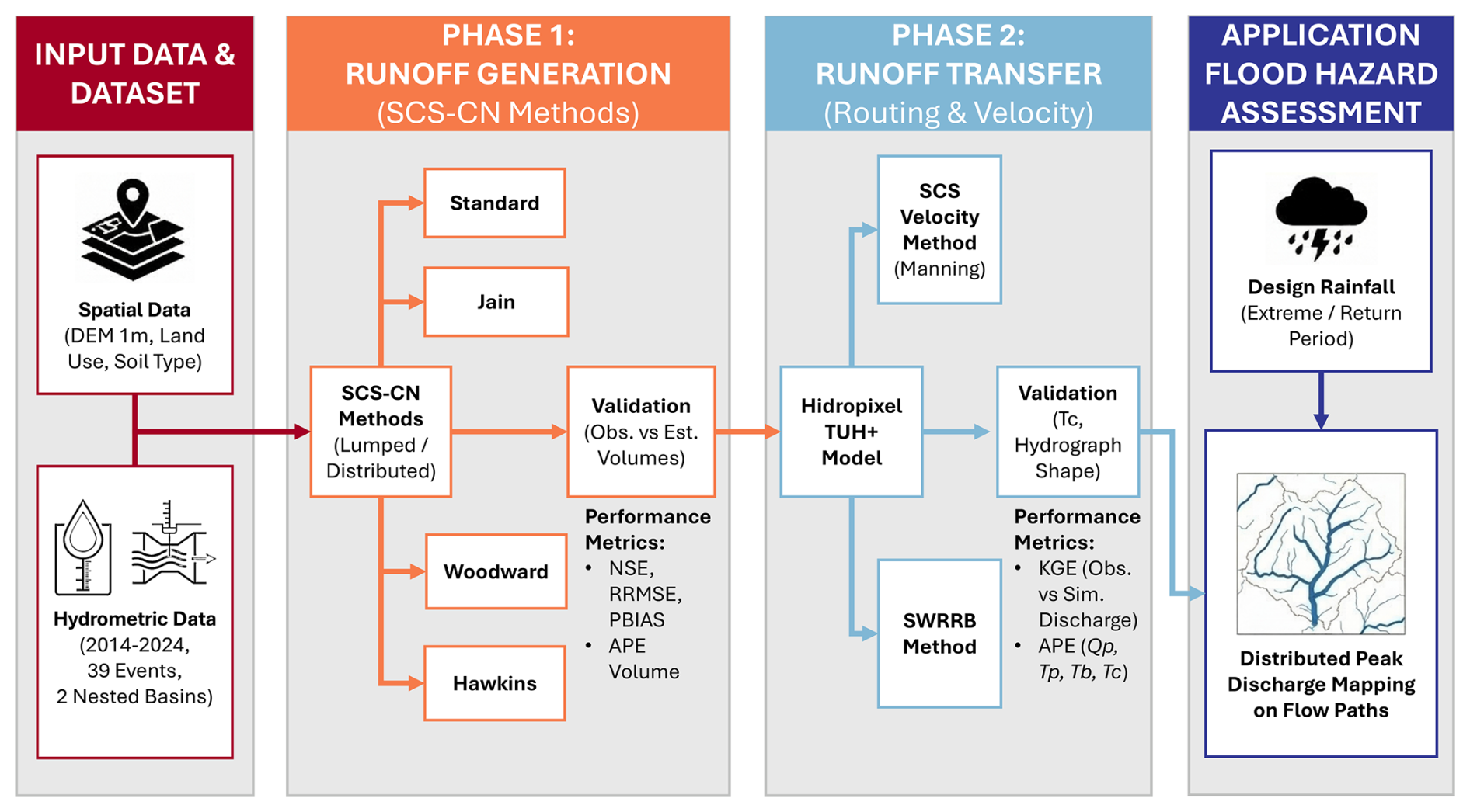
Figure 2 Schematic overview of the methodological framework implemented in this study.

Runoff transfer (Phase 2) is analysed by routing the excess rainfall generated with the best-performing SCS-CN formulation. This phase focuses on the temporal dynamics of the flow. Two distinct hydraulic strategies for estimating flow velocity and travel time are contrasted: the SCS velocity method and the SWRRB method. The validity of these routing schemes is determined by their capacity to predict T_c, T_p, and ultimately Q_p at the outlet.

Finally, the framework integrates these validated components to operationalize runoff flood hazard assessment. Using the optimal combination of production and transfer functions, the method generates a distributed map of Q_p along concentrated flow paths. To achieve this, the Hidropixel model is computationally optimized to be applied iteratively to every pixel along the defined concentrated flow paths, treating each as an independent outlet. This allows for a precise, localized quantification of flood hazard at a high spatial resolution.

2.3 The Hidropixel modelling framework

Fundamentally, Hidropixel (Lima et al., 2024) discretizes the catchment into a regular grid, treating each pixel as an independent micro-basin. The operational structure of the model follows four sequential steps (Fig. 3): (1) the estimation of excess runoff per pixel, (2) the calculation of hydraulic travel time, (3) the routing of runoff using the TUH+ approach, and (4) the superposition of individual pixel hydrographs at the outlet. The specific mathematical formulations compared in this study for the generation (step 1) and transfer (steps 2 and 3) phases are detailed in the following subsections.

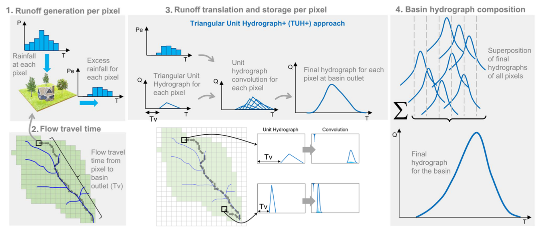
Figure 3 Schematic illustration of the Hidropixel model (based on Lima et al., 2024).

2.3.1 Runoff generation per pixel: SCS-CN method and variants

Consistent with standard event-based SCS-CN applications (e.g., Costa et al., 2019; Lima et al., 2024), the framework restricts routing to surface pathways, omitting a subsurface component to maintain model parsimony. In the specific context of compacted or crusted agricultural soils, rapid pluvial flood peaks are overwhelmingly dominated by surface runoff, making subsurface contributions to the extreme peak negligible (Beven, 2012; Cerdan et al., 2004; Evrard et al., 2008). The model's initial module calculates effective rainfall volume at the pixel scale using the SCS-CN method. The CN is derived from the available data: land use, hydrologic soil group, and antecedent moisture conditions. A normal state (CNII) is assumed for all simulations, rather than applying a dynamic adjustment based on the traditional 5 d antecedent precipitation (P5) index. This fixed approach aligns with updated guidance and recent evidence demonstrating that the discrete P5 correction is a poor surrogate for the actual catchment conditions controlling runoff response (Hawkins et al., 2008; Palli-Gravani et al., 2026; Soulis, 2018; Soulis and Valiantzas, 2012; USDA-NRCS, 2010).

The SCS-CN equations estimate surface runoff (Q) as a function of total precipitation (P) and the potential maximum retention (S), as defined by Eqs. (1)–(3):

$$\begin{array}{}\text{(1)}& {\displaystyle }Q=\left\{\begin{array}{ll}\frac{{\left(P-I_{\mathrm{a}}\right)}^{\mathrm{2}}}{P-I_{\mathrm{a}}+S}& \text{when}P>I_{\mathrm{a}}\\ \mathrm{0}& \text{when}P\le I_{\mathrm{a}}\end{array}\right.\text{(2)}& {\displaystyle }{I}_{\mathrm{a}}=\mathit{\lambda }S\text{(3)}& {\displaystyle }S={\displaystyle \frac{\mathrm{25}\mathrm{400}}{\mathrm{CN}}}-\mathrm{254}\end{array}$$

where P, Q, I_a (initial abstraction), and S are expressed in mm. In the standard method, I_a is conceptually linked to storage by a fixed ratio, λ.

Modifying λ requires adjusting S, as standard CN tables were originally calibrated for λ=0.2. To identify the most accurate approach for ungauged conditions, this study evaluates four distinct SCS-CN formulations:

1. Standard Method (λ=0.2): The classical approach using the original unadjusted S derived from standard CN tables.

2. Hawkins Method (λ=0.05): This approach adopts a reduced λ and adjusts the relationship between S_0.05 and the standard S_0.2 using the linear conversion proposed by Hawkins et al. (2008):

   $$\begin{array}{}\text{(4)}& S_{\mathrm{0.05}}=\mathrm{1.42}{S}_{\mathrm{0.2}}\end{array}$$

3. Woodward Method (λ=0.05): This method employs a non-linear conversion derived by Woodward et al. (2003) from a large dataset of 28 301 events across 307 US catchments (with S expressed in mm):

   $$\begin{array}{}\text{(5)}& S_{\mathrm{0.05}}=\mathrm{0.8187}(S_{\mathrm{0.2}}{)}^{\mathrm{1.15}}\end{array}$$

4. Jain Method: Unlike the previous methods, which assume a constant $I_{\mathrm{a}}/S$ ratio, Jain et al. (2006) proposed a generalized relation where I_a depends on P relative to S. Calibrated on 22 392 events, this formulation showed superior performance with parameter values of λ=0.3 and α=1.5:

   $$\begin{array}{}\text{(6)}& I_{\mathrm{a}}=\mathit{\lambda }S{\left({\displaystyle \frac{P}{P+S}}\right)}^{\mathit{\alpha }}\end{array}$$

Each of the four SCS-CN derivations is evaluated under two configurations: a classic lumped application, where the CN is area-weighted at the basin scale, yielding a uniform runoff depth, and a distributed application within Hidropixel.

2.3.2 Flow travel time

Once the runoff volume is generated, the model determines the time required for a water particle to travel from each pixel to the catchment outlet (T_v). Addressing the specific recommendation by Veeck et al. (2020) to explore alternative routing formulations in Hidropixel, this study evaluates two indirect hydraulic formulations for estimating travel time: (a) the distributed SCS velocity method, which is the standard Hidropixel approach, and (b) the SWRRB method. In addition, (c) an intensity-dependent adjustment of T_v is applied to extreme events (T>2 years) to account for faster flow velocities during heavy rainfall.

SCS velocity method

The SCS velocity method segments the flow path into three distinct regimes based on hydraulic thresholds: sheet flow, shallow concentrated flow, and open channel flow (USDA-NRCS, 2010). Sheet flow is assumed to occur over the first 30 m of the hillslope, where travel time (T_s) is calculated by Eq. (7) using a kinematic wave approximation sensitive to surface roughness. Within the SCS-TR55 framework (USDA-NRCS, 2010), this 30 m length serves as a standardized empirical upper bound for initial overland flow before water concentrates into rills. Although true physical sheet flow is rare in undisturbed environments like forested catchments, it occurs frequently in the agricultural areas studied here, where soil compaction and crusting significantly reduce infiltration and favour diffuse runoff. Beyond this distance, flow transitions to shallow concentrated flow (e.g., rills and gullies), where velocity is a function of the square root of the slope (Eq. 8). To prevent unrealistic flow velocities in steep terrain, velocities are explicitly bounded between 0.02 and 2.0 m s⁻¹ following Grimaldi et al. (2010). Finally, open channel flow is modelled using Manning's equation within the permanent drainage network (Eq. 9). The total travel time for any given pixel i is calculated by summing the transit times of all successive cells along the hydraulic flow path to the outlet (Eq. 10).

$$\begin{array}{}\text{(7)}& {\displaystyle }{T}_{{\mathrm{s}}_i}={\displaystyle \frac{\mathrm{5.474}(L_i{n}_i{)}^{\mathrm{0.8}}}{P_{\mathrm{24}}^{\mathrm{0.5}}{I}_i^{\mathrm{0.4}}}}\text{(8)}& {\displaystyle }{T}_{{\mathrm{sc}}_i}={\displaystyle \frac{L_i}{V_i}},\text{where}{V}_i=k_i{I}_i^{\mathrm{0.5}}\text{(9)}& {\displaystyle }{T}_{{\mathrm{cc}}_i}={\displaystyle \frac{L_i}{V_i}},\text{where}{V}_i={\displaystyle \frac{{\mathrm{Rh}}_i^{\mathrm{2}/\mathrm{3}}{I}_i^{\mathrm{1}/\mathrm{2}}}{n_i}}\text{(10)}& {\displaystyle }{T}_{{\mathrm{v}}_i}={\sum }_{i=\mathrm{1}}^{N_s}{T}_{{\mathrm{s}}_i}+{\sum }_{i=\mathrm{1}}^{N_{\mathrm{sc}}}{T}_{{\mathrm{sc}}_i}+{\sum }_{i=\mathrm{1}}^{N_{\mathrm{cc}}}{T}_{{\mathrm{cc}}_i}\end{array}$$

where $T_{{\mathrm{v}}_i}$ is the total travel time of the ith pixel (min), representing the sum of travel times across the operative flow regimes: sheet flow ($T_{{\mathrm{s}}_i}$), shallow concentrated flow ($T_{{\mathrm{sc}}_i}$), and open channel flow ($T_{{\mathrm{cc}}_i}$). L_i is the flow length across the pixel (m), corresponding to the pixel side length for orthogonal flow, or $\sqrt{\mathrm{2}}$ times the side length for diagonal flow directions; V_i is the pixel velocity (m s⁻¹); I_i is the pixel slope (m m⁻¹); P₂₄ is the rainfall depth for the 24 h duration and 2-year return period (mm); n_i is the pixel-specific Manning's roughness coefficient; k_i is a local routing coefficient derived from the simplification of Eq. (9), assuming a constant hydraulic radius and roughness for specific land covers under a wide-channel hypothesis (USDA-NRCS, 2010); Rh_i is the hydraulic radius (m) of the ith pixel, defined as the ratio of the cross-sectional area of flow to its wetted perimeter; and N represents the number of downstream pixels in each respective flow regime. Importantly, P₂₄ does not represent the specific storm being simulated. Following the TR-55 derivation (McCuen, 2004), P₂₄ acts solely as a fixed, localized geographic constant to approximate baseline rainfall intensity for sheet-flow travel time.

In the NRCS formulation, shallow concentrated flow velocity is estimated assuming a constant flow depth of approximately 7.6 cm (0.25 ft), or up to 12.2 cm (0.4 ft) for grassed waterways (USDA-NRCS, 2010). While this assumption is suitable for coarse-resolution digital elevation models (DEMs) (e.g., 30 m) where micro-topography is smoothed, it becomes inconsistent in high-resolution modelling of dry valleys. Indeed, refining DEM resolution (i.e. reducing cell size) inevitably extends flow path lengths (Grimaldi et al., 2012; Moglen and Hartman, 2001). Without a corresponding adjustment in hydraulic parameters, this mechanical increase in path length leads to a systematic overestimation of travel times. Furthermore, in the specific context of Walloon dry valleys, the shallow flow regime often extends over significant distances. Treating these zones with a fixed, shallow depth fails to account for the progressive concentration of flow and the associated increase in hydraulic radius.

Field observations from the Chastre experimental catchment confirmed that flow depths progressively increase as runoff concentrates, reaching 14 cm at a 4 ha sub-catchment outlet and exceeding 70 cm within the main terminal channel of the 111 ha basin. To accurately represent this geomorphological continuum from hillslope runoff to channelized flow, the constant 7.6 cm shallow depth assumption was empirically adjusted. A site-specific, stepwise area-to-depth relationship was calibrated based on the contributing area (Ac):

• Ac < 5 ha: 7.6 cm (Standard shallow concentrated flow)

• 5 ≤ Ac < 50 ha: 12.2 cm (Deepening concentrated flow)

• 50 ≤ Ac < 100 ha: 20.0 cm (Transition to open channel flow)

• Ac ≥ 100 ha: 30.0 cm (Established open channel flow)

This local reclassification represents the transition from shallow to channel flow. It overcomes the limitations of the fixed shallow routing coefficient (k) in high-accumulation thalwegs, ensuring a more realistic routing process consistent with local observations.

SWRRB method

As an alternative to the distributed NRCS approach, the SWRRB method (Williams et al., 1985) offers a semi-empirical formulation commonly used in basin-scale models. SWRRB estimates the total time for each pixel as the aggregate of a hillslope component ($T_{{\mathrm{s}}_i}$), dependent on sheet flow characteristics, and a channel component ($T_{{\mathrm{cc}}_i}$), which is a function of the basin's morphometry. This method is tested here to evaluate whether a simplified routing scheme can perform adequately within a high-resolution modelling framework. The hillslope travel time (Eq. 11) and channel travel time (Eq. 12) are calculated as follows:

$$\begin{array}{}\text{(11)}& {\displaystyle }{T}_{{\mathrm{s}}_i}={\displaystyle \frac{(L_i{n}_i{)}^{\mathrm{0.6}}}{\mathrm{18}{I_i}^{\mathrm{0.3}}}}\text{(12)}& {\displaystyle }{T}_{{\mathrm{cc}}_i}={\displaystyle \frac{\mathrm{0.62}{L}_{{\mathrm{c}}_i}{n_i}^{\mathrm{0.75}}}{{A_i}^{\mathrm{0.125}}{I_i}^{\mathrm{0.375}}}}\text{(13)}& {\displaystyle }{T}_{{\mathrm{v}}_i}=T_{{\mathrm{s}}_i}+T_{{\mathrm{cc}}_i}\end{array}$$

The method is applied using averaged parameters for each flow type. The variables are defined as follows: $T_{{\mathrm{s}}_i}$ and $T_{{\mathrm{cc}}_i}$ represent the travel times (h) across the ith pixel for sheet flow and open channel flow, respectively; L_i is the flow length (m); $L_{{\mathrm{c}}_i}$ is the channel length (km); n_i represents the Manning's roughness coefficient averaged along the flow path L; I_i is the average slope of the flow path L (m m⁻¹), calculated as the total elevation difference divided by the flow length L; A_i corresponds to the drainage area of the outlet considered (km²).

As in the SCS velocity method, a flow length threshold of 30 m separates sheet flow from concentrated flow, since sheet flow rapidly concentrates into rills owing to micro-topographic irregularities (McCuen and Spiess, 1995; USDA-NRCS, 2010).

Finally, to mitigate numerical artifacts associated with flat areas – which are more prevalent in high-resolution DEMs – a minimum slope of 0.005 m m⁻¹ is imposed for travel time calculations (Appendix A).

Adjustment of flow travel time

A critical physical limitation in static routing models is the assumption of constant flow velocity regardless of storm magnitude. However, for extreme events, flow velocities increase significantly due to greater flow depths. As demonstrated by Grimaldi et al. (2012) and Michailidi et al. (2018), flow velocities increase – and consequently, T_c decreases – as the return period (T) and rainfall intensity increase. Using a fixed T_v derived from frequent events (e.g., 2-year rainfall) would therefore underestimate Q_p for extreme storms (e.g., 100-year events).

To account for this non-linearity, this study adopts the kinematic wave scaling approach proposed by Meyersohn (2016). This method adjusts the reference travel time based on the ratio of effective rainfall intensities:

$$\begin{array}{}\text{(14)}& T_{\mathrm{v}}=T_{\mathrm{v},\mathrm{R}}{\left({\displaystyle \frac{E}{E_{\mathrm{R}}}}\right)}^m\end{array}$$

where T_v is the adjusted travel time for the specific T; T_v,R is the reference travel time calculated in the standard Hidropixel run (based on 2-year rainfall parameters); E is the effective rainfall intensity of the extreme event; E_R is the effective rainfall intensity of the reference event; m is a dimensionless kinematic wave parameter dependent on flow geometry.

Following Meyersohn (2016), the exponent m is set to −0.4 for sheet flow and wide rectangular paths (representing overland flow), and −0.3 for channel flow, assuming a trapezoidal channel geometry typical of the concentrated flow paths in the study area. Preliminary sensitivity tests conducted on extreme rainfall events within this specific catchment confirmed that incorporating this adjustment yields superior T_v restitution compared to static methods (data not shown).

2.3.3 Triangular unit hydrograph (TUH)

The final stage of the modelling framework converts the excess rainfall volume and travel time calculated for each pixel into a specific discharge response at the catchment outlet.

In this distributed framework, a specific TUH is generated for every pixel i. Central to the TUH+ enhancements (Lima et al., 2024), the travel time determined in the previous step drives the entire shape of the hydrograph. It influences not only the temporal delay (translation) but also the attenuation of the signal (storage). Pixels located further from the outlet, having larger T_v values, generate TUHs with longer time-to-peak and lower Q_p. This mechanism allows the model to physically represent the increased storage and diffusion effects associated with longer flow paths.

$$\begin{array}{}\text{(15)}& {\displaystyle }{T}_{{\mathrm{p}}_i}={\displaystyle \frac{d}{\mathrm{2}}}+\mathrm{0.6}{T}_{{\mathrm{v}}_i}\text{(16)}& {\displaystyle }{T}_{{\mathrm{b}}_i}=\mathrm{2.67}{T}_{{\mathrm{p}}_i}\text{(17)}& {\displaystyle }{Q}_{{\mathrm{p}}_i}=\mathrm{0.208}\left({\displaystyle \frac{A_i}{T_{{\mathrm{p}}_i}}}\right)\end{array}$$

In these expressions, the subscript i denotes the specific pixel index. The temporal parameters $T_{{\mathrm{p}}_i}$ (time-to-peak) and $T_{{\mathrm{b}}_i}$ (base time), along with the excess rainfall duration d, are expressed in hours (h). The peak discharge $Q_{{\mathrm{p}}_i}$ is expressed in m³ s⁻¹ per mm of excess rainfall and is proportional to the pixel area A_i (km²).

2.3.4 Final hydrograph for the catchment

The final hydrograph at the outlet is generated by convolving the excess rainfall volume (step 1) with the generated UH for each pixel (step 3). This step sums the individual contributions of every grid cell (N_p active pixels) across the catchment. By doing so, the flow is explicitly lagged by the travel time (step 2) and dispersed by the shape of the TUH transfer function, resulting in a spatially integrated runoff response.

$$\begin{array}{}\text{(18)}& Q_{\mathrm{tot}}\left(t\right)={\sum }_{i=\mathrm{1}}^{N_p}Q(t{)}_i\end{array}$$

2.3.5 Computational optimization for high-resolution modelling

Applying the distributed TUH+ approach at a 1 m resolution entails a substantial computational load, as the 111 ha study catchment is discretized into over a million active cells. A cell-by-cell convolution would be computationally prohibitive. To address this, a grouped convolution strategy is implemented. The algorithm identifies unique combinations of CN and T_v across the catchment. Instead of computing the convolution integral for every individual pixel, pixels sharing identical hydraulic properties (CN) and routing delays (T_v) are aggregated into a single computational unit. The UH is generated once for each unique (CN, T_v) pair and subsequently scaled by the total contributing area of the associated cluster. This approach reduces the number of required operations by several orders of magnitude, making the 1 m resolution modelling feasible without compromising the fully distributed nature of the results.

To maximize the efficiency of the grouping algorithm, the continuous variables are discretized: CN and T_v values are rounded to the nearest integer, thereby reducing the number of unique computational pairs.

This rounding step was validated on a subset of 29 events (Point 2) and found to introduce negligible error (mean ΔQ_p=0.50 ± 0.81 L s⁻¹; Nash-Sutcliffe Efficiency (NSE) = 0.999 between rounded and unrounded hydrographs) while substantially reducing computation time.

Simulations were run in Python 3.11 on a standard workstation (32 GB RAM). The 39 events at the two outlets take under 5 min in total, and the full spatialized application along the concentrated flow paths (Sect. 2.4.2; 1.11 million active cells, 8689 temporary outlets) takes ∼ 2 min per storm via the grouping procedure. Benchmarks on four larger Walloon catchments (1500 to 4000 ha) and a stress test on the catchment at Flobecq (198 min for a single storm; Appendix B) indicate the approach remains computationally tractable beyond the experimental catchment, though it highlights the importance of adapting the spatial resolution to the target area (Appendix B).

2.4 Calculation of pluvial flood hazard: spatialization of peak flows

2.4.1 Rainfall

To drive the rainfall scenario simulations, the meteorological forcing is represented by a double-triangle design storm hyetograph, a standard methodological approach developed in France (Chocat et al., 1981). The temporal distribution of this synthetic storm relies on site-specific Montana coefficients, which are officially available at the municipal scale for the entire territory (https://www.meteo.be/fr/climat/climat-de-la-belgique/climat-dans-votre-commune, last access: 19 October 2026), to specifically calculate and construct the dual-intensity peaks, providing a standardized critical rainfall profile for unmonitored areas.

2.4.2 Pluvial flood susceptibility map

Unlike traditional lumped approaches that provide hydrographs solely at the basin outlet, this framework extends the modelling scope to map peak discharge, used here as a hydrological indicator of pluvial hazard, across the entire catchment. The model computes Q_p for every pixel located along the identified concentrated flow paths, which were delineated using a minimum flow accumulation threshold of 0.5 ha. In this procedure, the routing algorithm iterates through the drainage network, treating each pixel as a temporary outlet that aggregates the runoff from its specific upstream contributing area. This allows for the identification of critical discharge points often missed by standard outlet-focused simulations.

Technically, this is implemented by dynamically offsetting the global travel time map relative to the target location. For every target pixel considered as a temporary outlet, the global travel time map is adjusted by subtracting $T_{{\mathrm{v}}_i}$ of that specific target pixel from the total travel time values of all upstream contributing pixels. This operation effectively resets the downstream boundary condition (T_v=0) to the location of the target pixel, simulating it as the new unique outlet for the convolution process.

While fully resolved hydraulic hazard mapping requires variables such as water depth and velocity, relying on spatially distributed Q_p provides a robust susceptibility indicator for rapid pluvial flooding. This choice directly aligns with current Walloon regulatory practice, which officially evaluates pluvial flood hazard through the combination of Q_p and rainfall return periods. Furthermore, because the proposed framework computes the full hydrograph, not merely the peak, at every active pixel, it preserves the temporal dynamics and flow duration necessary to derive alternative hazard indices if required. Applying this susceptibility mapping at the scale of small headwater catchments (e.g., 111 ha) addresses a critical operational need: in the Belgian loess belt, rapid surface runoff and muddy flows originating from these agricultural areas constitute the predominant regional flood risk, frequently surpassing traditional fluvial flooding in both frequency and impact (Evrard et al., 2008).

2.5 Application of the model

2.5.1 DEM pre-processing

The primary topographical input for this study is the high-resolution LiDAR DEM covering the Walloon region of Belgium (2021–2022, available on https://geoportail.wallonie.be, last access: 19 October 2026). Originally acquired at a 0.5 m resolution, the data were aggregated to 1 m. A critical aspect of distributed modelling is the sensitivity to DEM resolution. While the Hidropixel framework has demonstrated robustness at coarser scales (10 to 30 m), the increasing availability of high-resolution LiDAR data offers the opportunity to model flow paths with metre-scale precision. However, this increase in resolution presents a trade-off: as noted by Tarolli (2014), ultra-high resolutions can introduce excessive noise from micro-topographic artifacts without necessarily yielding proportional hydrological gains. In the specific context of Hidropixel, Veeck et al. (2020) analysed scale dependencies. They confirmed that, while coarser resolutions smooth out Q_p, finer grids are essential for capturing realistic travel times and flow connectivity. These observations align with findings by Thomas et al. (2017) and Cantreul et al. (2018), who identify the 1 m threshold as an optimum for delineating hydrologically sensitive zones while avoiding over-sensitivity to micro-topographic variations. Furthermore, Alexopoulos et al. (2024) recently demonstrated a sharp degradation in hydraulic accuracy when coarsening grids from 1 to 5 m. Consequently, this study adopts a 1 m resolution to best represent flow path variability while maintaining computational feasibility (Murphy et al., 2008; Vaze et al., 2010).

While the computational grid operates at 1 m to capture topographic routing and connectivity with maximum fidelity, inputs like land use (2 m) and soil (10 m) are intrinsically coarser. The 1 m grid acts as a high-resolution topographic framework rather than implying metre-scale knowledge of all parameters. A resolution-sensitivity analysis (1, 2, 5, 10 m; Appendix A) confirms its necessity: 5 to 10 m grids artificially smooth topography, overestimating Q_p by 25 % to 28 %. However, a 2 m grid provides a viable operational compromise for wider regional applications.

To simulate surface runoff, the raw DEM must be pre-processed to ensure hydrological continuity (i.e., removal of sinks and digital dams) (Jenson and Domingue, 1988; O'Callaghan and Mark, 1984). However, applying standard “sink filling” algorithms to high-resolution topography is known to introduce significant artifacts. As noted by Lidberg et al. (2017), pure filling tends to create artificial flat surfaces and linear flow paths that deviate from natural drainage patterns.

To mitigate these artifacts, a composite hydro-conditioning workflow was implemented using the WhiteboxTools geospatial library (Lindsay, 2016). Instead of relying solely on filling, this approach prioritizes breaching (lowering channel obstructions) to preserve the natural nuances of the landscape.

2.5.2 Land use and soil properties

To accurately characterize surface roughness and runoff potential, a composite land use map was generated by merging two complementary high-resolution datasets.

• The primary source for arable land is the Land Parcel Identification System (SIGEC). This vector dataset provides an annual inventory of declared agricultural parcels, distinguishing between specific crop types, productive arable land, and non-productive features such as permanent grasslands, fallows, and grass buffer strips (https://geoportail.wallonie.be, last access: 19 October 2026).

• For non-agricultural areas, the LifeWatch Wallonia land cover map (Radoux et al., 2022) is used at a 2 m spatial resolution to capture the remaining topographic features (forests, urban areas, water bodies).

Hydrological parameters (CN, Manning's n) associated with general land cover classes are detailed in Table 1, derived from standard literature (Chow et al., 1988; Schneider and McCuen, 2005; SCS, 1972; USDA-NRCS, 2010). Given the high granularity of the SIGEC dataset, which contains more than 150 distinct crop classes, the full lookup table is not presented here. However, specific values for these crops were assigned using USDA-NRCS (2010), supplemented by CN values from the EPICgrid model (Sohier et al., 2009).

Table 1 Summary of model parameters. The table presents Curve Number (CN) values cross-referenced by land use and Hydrologic Soil Group (A–D), alongside Manning's roughness coefficients (n) categorized by flow type.

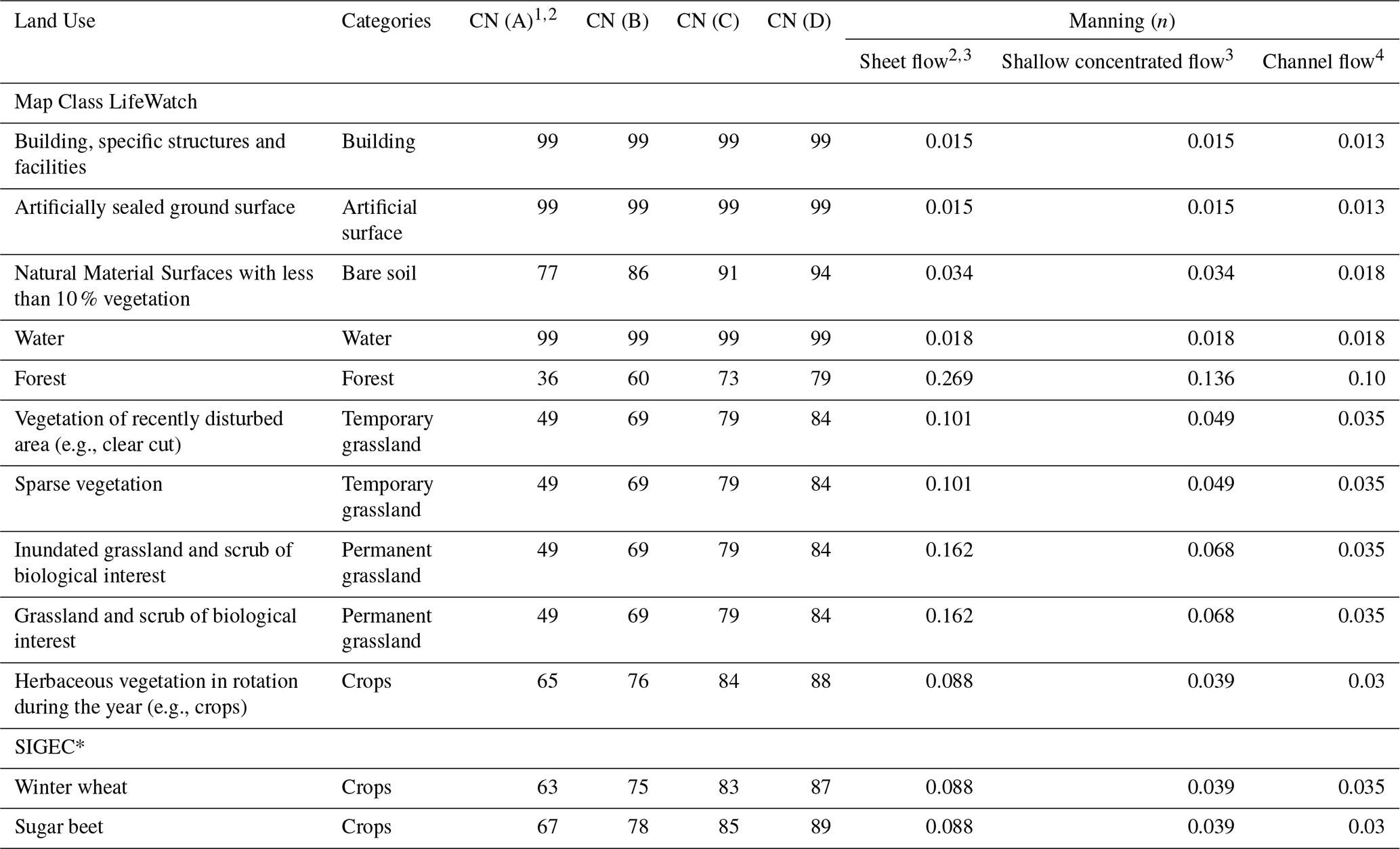
¹ Sohier and Degré (2011); ² USDA-NRCS (2010); ³ McCuen et al. (1996); ⁴ Chow (1959). * Non-exhaustive list.

The Hydrologic Soil Groups required for the CN method are derived from the Walloon soil infiltrability map (Demarcin et al., 2011). This dataset classifies soils into four standard groups (A, B, C, and D) based on their minimum infiltration rate, which is determined by pedological characteristics including soil texture, depth to bedrock, stratification, and natural drainage capacity.

2.5.3 Hydrometeorological data and event selection

To evaluate the models, a monitoring dataset was compiled from the experimental watershed at Chastre (encompassing sub-catchments Point 2 and Point 3; see Sect. 2.1). The precipitation data were recorded using a high-precision weighing rain gauge (OTT Pluvio² L) located near the outlet of the 84 ha sub-catchment (Point 2). This device provides data at a 5 min temporal resolution, ensuring accurate capture of peak intensities.

Coincident streamflow series were derived from a continuous monitoring network adapted to local channel morphologies. Runoff at controlled outlets was monitored using gauging flumes (e.g., San Dimas type), where water levels were converted to discharge using site-specific stage-discharge relationships. For simple channel sections without structural controls, discharge was continuously computed by coupling water level measurements with acoustic Doppler velocity sensors. All discharge datasets were recorded and synchronized with rainfall data at a 5 min time step to ensure precise lag-time analysis.

The study utilizes a total of 39 rainfall-runoff events recorded between 2014 and 2024 (Table C1), comprising 29 events at the 84 ha outlet and 10 at the 111 ha outlet. To ensure hydrological relevance, events were included only if they met a minimum total rainfall depth of 2.5 mm and generated measurable discharge at either gauging station. Although regional studies (Laurant and Bollinne, 1976) indicate that runoff can initiate at depths as low as 1.27 mm under optimal conditions (wet soils, bare land), a conservative 2.5 mm threshold, roughly twice this baseline, was adopted to guarantee consistent and significant runoff generation regardless of initial moisture or vegetation states. In addition, the analysis was restricted to short-duration rainfalls (<24 h) to align with the fundamental assumption of the standard SCS-CN method, which is designed for single-event simulations and inherently neglects continuous inter-storm drainage and evapotranspiration processes (Mishra and Singh, 2003; Ponce and Hawkins, 1996).

The return period of each storm was determined based on the total amount and duration of the rainfall events using the official Intensity-Duration-Frequency (IDF) curves for the catchment location (Royal Meteorological Institute of Belgium, RMI). Out of the 39 events, 35 events are hereafter considered as normal events (T<2 years) whereas 4 events with T≥2 years will be referred to as extreme events.

To evaluate the indirect routing configurations (SCS and SWRRB, see Sect. 2.3.2), a reference T_c, defined as the travel time from the hydraulically most distant pixel to the catchment outlet, is derived directly from the observed rainfall-runoff events. This study employs the inflection point method to define T_c as the time interval between the cessation of effective rainfall and the inflection point on the hydrograph's recession limb (Gericke and Smithers, 2014; McCuen, 2009).

Identifying this point is critical in the specific context of the studied dry valleys. Since the hydrological regime is ephemeral (Q_base≈0), baseflow separation is not required. However, determining the exact cessation of direct runoff remains challenging due to the asymptotic nature of the recession curve, which reflects slow channel depletion. To resolve this, the inflection point is identified by analysing the second derivative of the smoothed discharge time series (${\mathrm{d}}^{\mathrm{2}}Q/\mathrm{d}{t}^{\mathrm{2}}=\mathrm{0}$). This provides a physically based indicator that marks the transition from active surface runoff contributions to the passive draining of channel storage (Nejadhashemi et al., 2007).

In practice, the raw discharge time series is smoothed prior to differentiation using a Savitzky-Golay filter (second-order polynomial, 15 min window), and the second derivative is evaluated on the smoothed series to identify the sign change marking the inflection point. While this algorithmic procedure removes the subjectivity of manual graphical extraction, the resulting T_c estimate remains sensitive to the choice of smoothing window: sensitivity tests varying the window from 10 to 25 min indicate a typical T_c variation of about ±10 %, which can be regarded as an approximate uncertainty bound on the reported concentration times.

2.5.4 Model performance evaluation criteria

As recommended in the literature (e.g., Fentie et al., 2002; Moriasi et al., 2015), a multi-criteria approach was adopted to ensure a comprehensive evaluation of the hydrological model performance. The Kling-Gupta Efficiency (KGE; Kling et al., 2012) serves as the primary goodness-of-fit statistic, providing a balanced assessment of correlation, variability, and bias. This is complemented by the NSE to evaluate overall hydrograph agreement, the Relative Root Mean Square Error (RRMSE) to quantify the residual variance, and the Percent Bias (PBIAS) to identify any systematic over- or underestimation tendencies.

Although these 39 events are evaluated as a single comprehensive dataset to assess overall model performance, records from these nested stations are not strictly independent. Accordingly, all statistical comparisons between methods are based on paired, non-parametric tests (e.g., Wilcoxon signed-rank) rather than assuming independent observations.

Furthermore, to evaluate the overall accuracy of the hydrograph reproduction, four event-based metrics are computed. While the relative volume error (δV) assesses the total runoff generation, the quality of the routing process is specifically measured by the relative time-to-peak error (δT_p) and base time error (δT_b), which reflect temporal synchronization and flow attenuation. The relative peak discharge error (δQ_p) evaluates the resulting flood magnitude. All four metrics are expressed as the normalized difference between simulated and observed values.

Taken together, the parameters underlying this framework differ in how directly they depend on the present dataset. CN values by land use and hydrologic soil group, the Jain initial abstraction ratio (λ=0.3, α=1.5), and the Manning's roughness coefficients were taken unchanged from published sources (Jain et al., 2006; USDA-NRCS, 2010). The minimum slope threshold (0.005 m m⁻¹; Sect. 2.3.2) was inferred from local field observations of thalweg slopes. The area-to-depth relationship for shallow concentrated flow (Sect. 2.3.2) and the extreme-event travel-time adjustment (Eq. 14) were tuned against locally observed hydrographs. The generic sheet-flow/shallow-concentrated/channel-flow hydraulic thresholds (USDA-NRCS, 2010) were, by contrast, applied without further local evaluation. Consequently, the framework relies on a hybrid parameterization strategy that combines robust literature defaults with targeted local constraints to ensure physical realism.

3 Results and discussion

3.1 Runoff generation

The evaluation of runoff volume generation, summarized in Table 2 and illustrated by the error distributions in Fig. 4, reveals significant disparities depending on the chosen volumetric method and, to a lesser extent, the spatial modelling approach.

The analysis of efficiency criteria highlights the inadequacy of the Standard (SCS-CN) method for this catchment. With an average negative NSE of −0.32 and a bias of −91 %, this method leads to a severe systematic underestimation of flow volumes. Figure 4 corroborates this by showing an error distribution collapsed towards −100 %, with a high density of crosses. These markers indicate that the precipitation depth did not exceed the initial abstraction (P < I_a), resulting in zero simulated runoff despite observed flow. This aligns with findings by Baltas et al. (2007) and Woodward et al. (2003), who demonstrated that the standard ratio (λ=0.2) tends to overestimate I_a in agricultural catchments, thereby preventing runoff initiation for low magnitude rainfall events.

Table 2 Performance metrics for runoff volume estimation across 39 events. Comparison of four volumetric methods (Standard, Hawkins, Woodward, Jain) applied to both distributed (Hidropixel) and lumped modelling frameworks. Bold values indicate the best performance for each metric.

Methods incorporating an adjusted λ – Woodward and Hawkins – improve upon the standard approach but still struggle with substantial volume deficits. While Woodward reduces the negative bias to approximately −71 %, Hawkins further mitigates the underestimation (bias near −60 %) and manages to produce slightly positive NSE values (up to 0.10). Although these approaches confirm the necessity of calibrating the I_a–S relationship rather than relying on default handbook values (Baltas et al., 2007; Baert et al., 2026), they remain insufficient for accurate volume restitution in this specific basin.

Conversely, the Jain method emerges as the best-performing approach for volume estimation among those tested. It achieves the highest overall performance, yielding the best NSE (0.17) and the lowest relative error (RRMSE of 133 %). Unlike the other methods that systematically underestimate runoff, the Jain method provides a much more balanced volume generation, displaying the smallest absolute bias (PBIAS = 16 %).

Furthermore, across all tested volumetric methods, the distributed Hidropixel model statistically outperforms the lumped approach (p<0.05, Wilcoxon signed-rank test), although the magnitude of this improvement is modest in absolute terms: for the best-performing (Jain) configuration, NSE rises from 0.14 to 0.17, RRMSE falls from 135 % to 133 %, and PBIAS improves from 19 % to 16 %. Quantitatively, the distributed framework yields higher NSE, lower RRMSE, and reduced bias, alongside error medians closer to zero and narrower interquartile ranges (Table 2; Fig. 4). While statistically detectable, this difference is better read as evidence of a modest but consistent benefit from spatially resolving the runoff process, rather than a substantial gain in predictive accuracy: explicitly accounting for the spatial heterogeneity of the CN allows for a more realistic identification of active contributing areas, whereas the lumped approach artificially dampens these localized responses through basin-wide averaging.

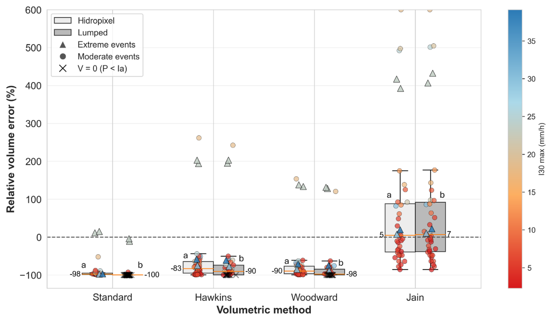
Figure 4 Comparative boxplots of signed relative volume error (%) for runoff events (n=39) at the Chastre watershed using the Hidropixel model (light grey) and a lumped model approach (grey). Marker shapes distinguish event categories (circles for normal events, triangles for extreme events), while the colour gradient indicates the I30 max (the maximum intensity of rainfall recorded over a period of 30 min), and the black crosses highlight zero-runoff simulations (P < I_a). Numeric median values are displayed. Different lowercase letters (a, b) indicate statistically significant differences between the distributed and lumped models (Wilcoxon signed-rank test).

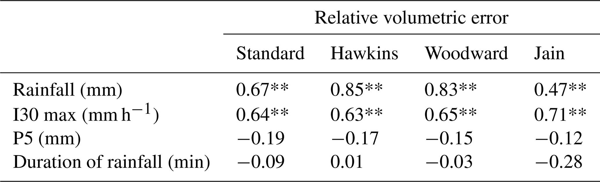
A deeper analysis using Spearman rank correlation dissects the drivers behind these performance disparities between methods (Table 3). For the Standard, Hawkins, and Woodward methods, the volumetric error exhibits a very strong, highly significant positive correlation with total rainfall depth (ρ=0.67 to 0.85). This indicates a structural bias where the error scales directly with storm size. The Jain method mitigates this issue, substantially reducing this dependency on total rainfall (ρ=0.47 vs. 0.67–0.85). This superiority stems from Jain's specific formulation, which explicitly incorporates the precipitation depth into the determination of the initial abstraction (Eq. 6). By making the abstraction dynamically dependent on the storm size rather than relying on a static linear ratio, the Jain method adapts much better to varying rainfall magnitudes. Interestingly, rainfall duration showed no significant correlation with volumetric error, further isolating intensity and volume as the primary meteorological drivers.

Table 3 Spearman rank correlation coefficients (ρ) between the relative volumetric error of the four SCS-CN configurations and key hydro-meteorological drivers. I30 max refers to the maximum intensity of rainfall recorded over a period of 30 min and P5 is the 5 d antecedent rainfall.

* p<0.05; ** p<0.01.

Spearman analysis reveals a persistent structural limitation across all methods: the error remains strongly correlated with the maximum 30 min rainfall intensity (I30max), peaking with Jain (ρ=0.71). This dependency exposes a well-known flaw in the classical SCS-CN framework, which relies solely on cumulative rainfall volume and ignores temporal intensity (Grimaldi et al., 2013; Ponce and Hawkins, 1996). Consequently, the model cannot distinguish between prolonged low-intensity rain and violent storms, structurally failing to capture Hortonian (infiltration-excess) runoff.

Beyond rainfall characteristics, the mixed performance is also plausibly driven by the model's structural inability to dynamically account for initial catchment conditions. In this study, all simulations were parameterized using a normal moisture state (CNII), deliberately excluding the traditional P5 adjustment. The Spearman analysis supports this decision, as P5 exhibited no significant correlation with the relative volume error. In line with updated guidelines, which discourage P5-based adjustments owing to their lack of statistical correlation with observed CN variations (Hawkins et al., 2008; USDA-NRCS, 2010), this result argues against P5-based CN adjustments. It is also consistent with a growing body of evidence showing that antecedent rainfall indices are poor surrogates for runoff generation. Instead, watershed heterogeneity and complex catchment conditions exert a far greater influence on runoff than simple antecedent-moisture classifications (Palli-Gravani et al., 2026; Soulis, 2018; Soulis and Valiantzas, 2012), indicating that P5 is an inappropriate basis for CN adjustment in event-based modelling. Consequently, the model operates entirely independently of the real pre-storm saturation level. As highlighted by Brocca et al. (2012) and Michel et al. (2005), without a continuous soil moisture accounting module to track the actual saturation deficit, the CN framework remains overly rigid. It introduces severe systematic biases whenever the assumed static CNII state misaligns with the true initial moisture conditions of the catchment.

This lack of temporal flexibility extends beyond short-term moisture to the seasonal scale. By utilizing a fixed annual CN, the model treats the catchment surface identically in winter (bare soil) and summer (fully developed canopy), entirely neglecting the evolution of crop cover and soil crusting. However, observed CNs exhibit distinct seasonal patterns, typically decreasing during the growing season as canopy interception and evapotranspiration increase (Hjelmfelt, 1991). While specific formulations exist to dynamically adjust the CN based on vegetation cover and crusting stages (e.g., Van Oost, 2003), they require highly localized and temporally continuous field data that are rarely available. Furthermore, as demonstrated in Appendix D (Fig. D1), applying these data-intensive dynamic adjustments to the present dataset did not yield superior performance compared to the Jain method.

In summary, the mixed performance of the model has a clear physical explanation: the static CN equation inherently struggles to reproduce runoff whenever the generation mechanism is dominated by highly dynamic factors – specifically rainfall intensity, variable antecedent moisture (which P5 captures poorly), and crop cover – that the conceptual framework does not explicitly resolve. While these structural limitations could invite a fundamental recalibration of the method (e.g., through context-specific adjustments of λ, as shown in Appendix D), such a pursuit would conflict with the objective of maintaining a parsimonious tool for ungauged basins, where the data required for more complex formulations are non-existent. Nonetheless, this framework offers a functional, low-parameterization alternative for poorly gauged or ungauged agricultural basins, where the calibrated approaches described above are not applicable. It should be noted that substantially higher predictive performance remains achievable on this same catchment when a more complex, locally calibrated production module is used: Baert et al. (2026) applied a threshold-controlled approach, optimizing event-specific initial abstraction ratios against observed rainfall-runoff responses and subsequently generalizing them via a regime-based clustering strategy, achieving a runoff-volume NSE of 0.94 over 154 events on the same 84 ha sub-catchment in diagnostic mode, whereas fixed and literature-based λ formulations reached a best NSE of only 0.13. This confirms that the modest performance reported here reflects the deliberate choice of a parsimonious production scheme using literature-based, non-locally-calibrated parameters, rather than an inherent ceiling on what this catchment's hydrological behaviour can support.

3.2 Runoff transfer

3.2.1 Comparison of time of concentration methods

As illustrated in Fig. 5, the response times for the two nested sub-catchments are remarkably similar, with median values of 50 and 55 min for Point 2 (84 ha) and Point 3 (111 ha), respectively. Given the 400 m channel distance separating these two outlets, this 5 min median delay translates to an average flow velocity of approximately 1.3 m s⁻¹, a realistic value for channel routing. However, T_c exhibits substantial inter-event fluctuation, ranging from roughly 15 to 85 min. Point 2 displays a wider dispersion, likely because its dataset encompasses a broader variety of seasonal configurations and rainfall intensities, whereas the usable events for Point 3 are characterized by greater meteorological and seasonal homogeneity.

The high standard deviation observed across events reflects the strong sensitivity of the catchment to dynamic variables, including rainfall intensity, spatial distribution of rainfall, and antecedent soil moisture. Statistically, the 5 d antecedent precipitation is the only factor showing a significant correlation with observed response times ($\mathit{\rho }=-{\mathrm{0.33}}^{*}$). This negative correlation indicates that wetter initial conditions tend to shorten T_c. This variability aligns with the findings of Langridge et al. (2020) based on an analysis of 1400 flood events in the UK. They demonstrated that high-intensity rainfall on saturated soils triggers a rapid hydrological response, whereas moderate rainfall on dry soils significantly elongates T_c. These observations suggest that characterizing the basin's response with a single, constant T_c parameter is physically limiting, highlighting the need for dynamic estimation methods.

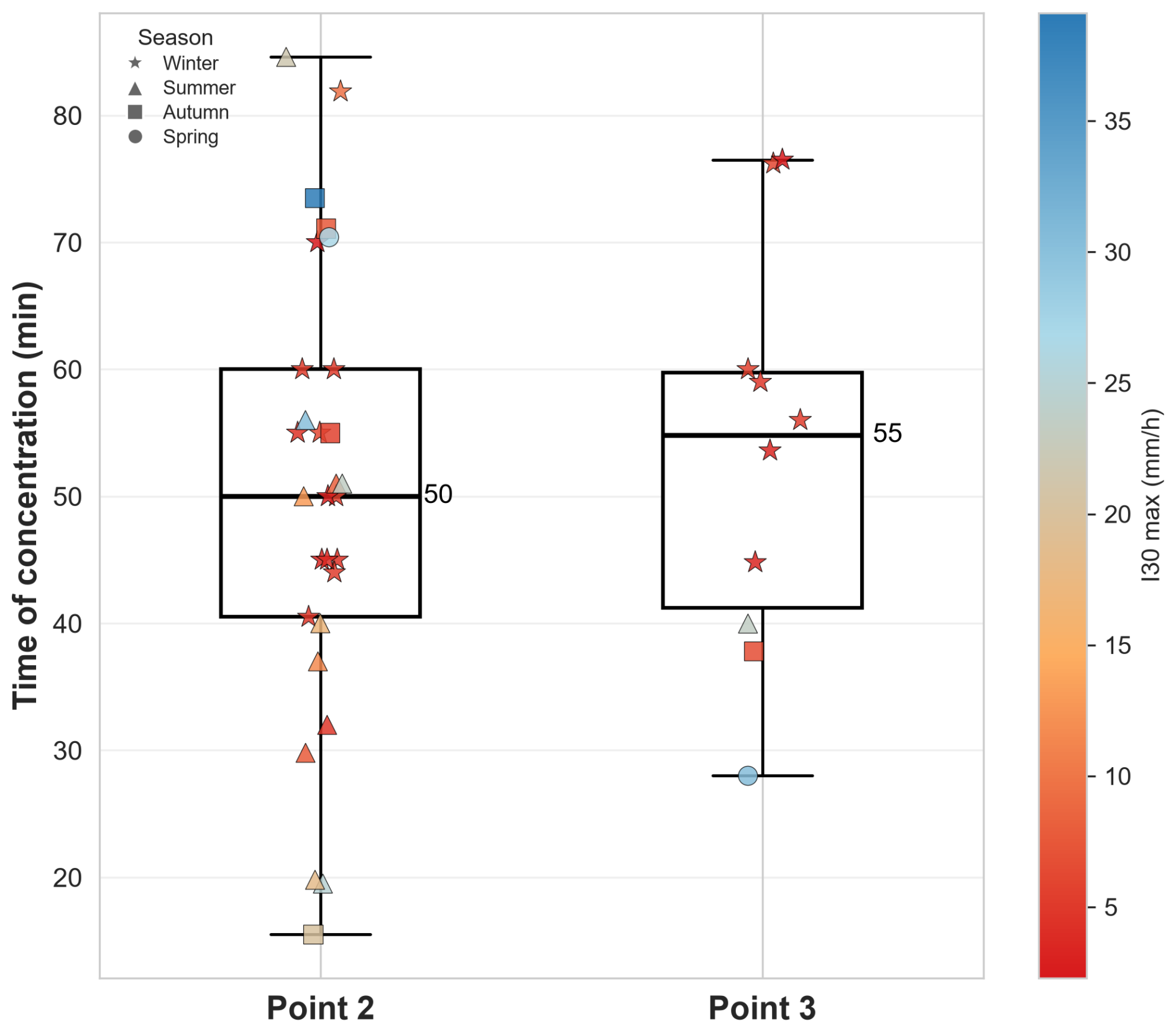
Figure 5 Comparative boxplots of observed concentration times at Point 2 (84 ha) and Point 3 (111 ha). Individual events are shown as markers, distinguished by season (symbol shape) and maximum 30 min rainfall intensity (I30max; colour gradient). Numerical median values are indicated.

Contrasting with this observed dynamism, the simulated travel time along the longest hydraulic path exhibits minimal variation across the 2014–2024 period. For both empirical methods (SCS velocity and SWRRB), inter-annual standard deviations remain below 1 min. Despite annual updates to the agricultural land use maps (SIGEC), the modelled hydraulic response remains static, which is likely explained by the limited discretization of roughness parameters. Assigning Manning's coefficients to broad categories like ”arable land” fails to distinguish between specific crop types, or the seasonal evolution of the canopy, thereby masking the actual hydraulic impact of the changing vegetation cover.

Temporal dynamics are poorly reproduced by both methods, which exhibit a persistent bias toward overestimating travel times. While median errors remain at 27 % for SWRRB and 38 % for SCS, maximum relative errors escalate to 300 % and 350 %, respectively (Fig. 6). These severe overestimations corroborate the observations of Grimaldi et al. (2012), who highlighted that static empirical formulas inherently produce very large uncertainties, often exceeding hundreds of percent, when applied to dynamic catchments. Although the SWRRB approach is significantly less biased than the SCS velocity method, both remain fundamentally limited. This is evidenced by a significant positive correlation between the relative T_c error and antecedent moisture ($\mathit{\rho }={\mathrm{0.34}}^{*}$). Because static models fail to capture the fact that larger runoff volumes – generated under wetter antecedent conditions – produce deeper and faster flows, their overestimation of travel times is systematically exacerbated as soil saturation increases. Consequently, accurate flow routing in agricultural catchments demands dynamic parameterization rather than rigid topographic equations.

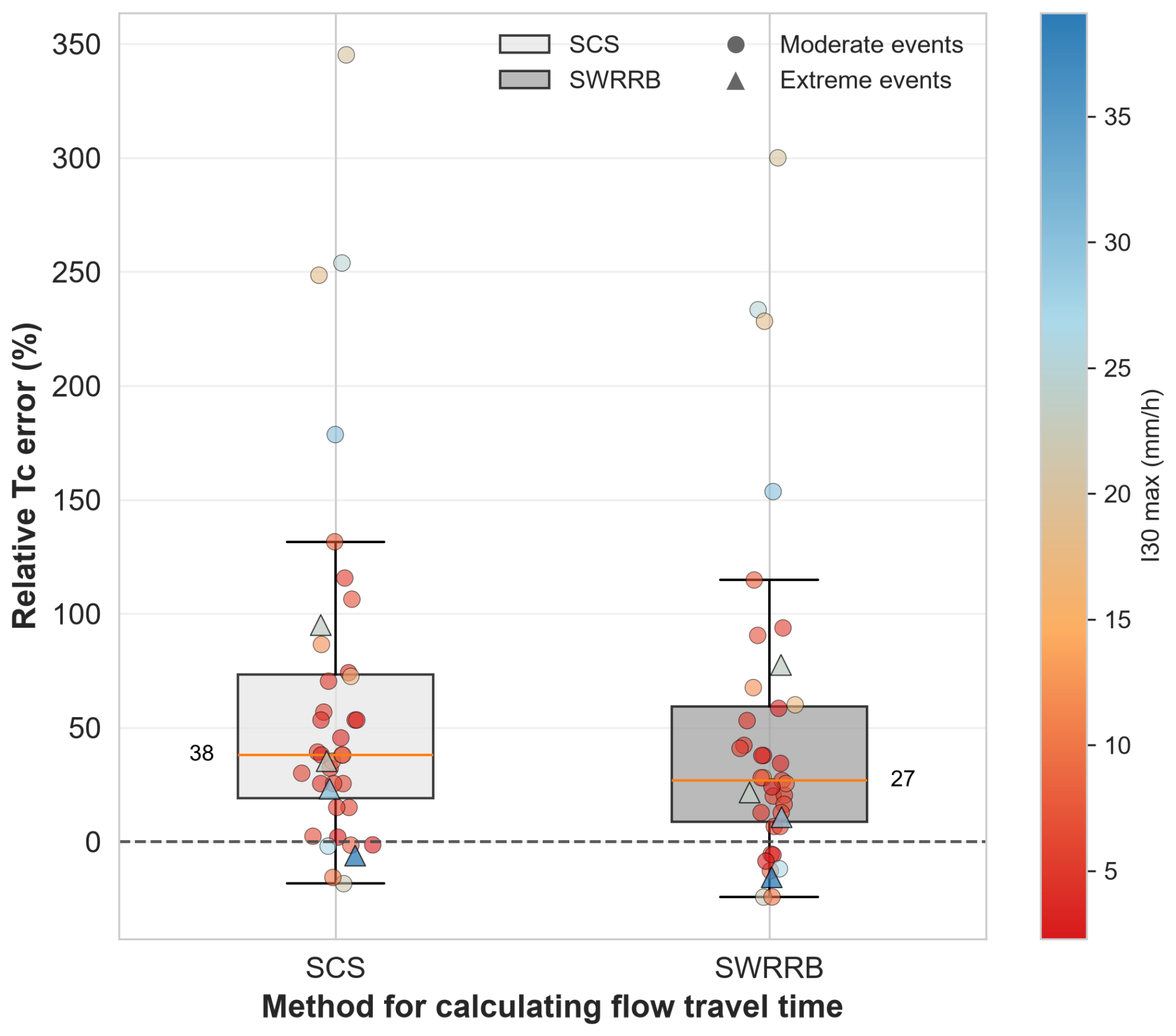
Figure 6 Distribution of relative errors (%) in time of concentration (T_c) estimation comparing the SCS velocity and SWRRB methods. Data points represent individual rainfall-runoff events (n=39), with the colour gradient indicating the maximum 30 min rainfall intensity. Numeric median values are displayed.

3.2.2 Spatial travel time patterns

Visually, the two methods generate different spatial patterns (Fig. 7). The SCS method yields a diffuse travel time map with smooth gradients and a less sharply defined dendritic network. This smooth spatial gradient stems directly from the method's distributed architecture, which relies on a cumulative, pixel-by-pixel summation. However, while this cumulative approach captures landscape heterogeneity, it introduces a high sensitivity to DEM micro-topography. A single pixel with a near-zero slope or high roughness acts as a hydraulic bottleneck, disproportionately inflating the accumulated travel time for the entire upstream contributing area. This structural sensitivity likely contributes to the systematic overestimation of T_c by the SCS method (Median error = 38 %; Fig. 6).

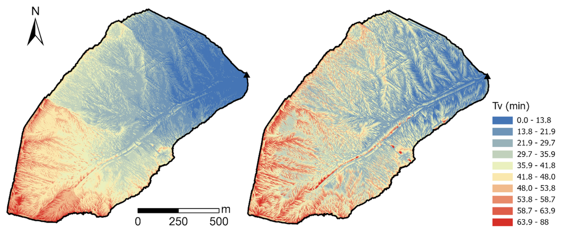
Figure 7 Spatial patterns of flow travel time (T_v) to the outlet calculated using the SCS velocity method (left) and the SWRRB method (right) for the year 2021 in the 111 ha basin (Point 3).

Conversely, the SWRRB method clearly delineates the network's dendritic structure with highly contrasted boundaries (Fig. 7, right). Unlike the cumulative SCS approach, SWRRB calculates the travel time for each cell based on path-averaged hydraulic parameters (slope, Manning's n) computed over distinct routing phases. Consequently, the sharp spatial gradients observed on the map do not reflect sensitivity to micro-topography, but rather mark the abrupt transitions between different flow regimes. Within a given flow type, the path-averaging technique acts as a spatial low-pass filter. Although this inherent smoothing may overlook small-scale hillslope retention features, it provides critical robustness against single-pixel DEM noise. The resulting map reveals structured preferential flow paths extending further upstream, ultimately producing a lower global T_c that better approximates the observed catchment dynamics (median error = 27 %; Fig. 6).

3.2.3 Limitations and sensitivity to scale

The SCS velocity method relies on empirical contributing area thresholds to proxy open channel initiation. While specifically calibrated for the Chastre catchment, relying solely on fixed drainage areas limits the method's transferability, as the transition to channelized flow is governed by complex geomorphological processes. To overcome this site-specificity, future frameworks could integrate more advanced channel initiation criteria. These include foundational slope-area thresholds (Montgomery and Dietrich, 1988), probabilistic approaches (Istanbulluoglu et al., 2002), and topographic metrics for gully development (Torri and Poesen, 2014; Wang et al., 2022). Incorporating such physically based criteria would refine automated flow regime classification and enhance spatial transferability.

While the comparison of methods highlights the relative robustness of the SWRRB method against micro-topographic noise, the interpretation of these results requires caution regarding the definition of T_c itself. Theoretically restricted to the longest hydraulic path, T_c reduces a distributed two-dimensional process to a one-dimensional metric. By ignoring the spatial variance of contributing areas, it characterizes a maximum potential travel time rather than the effective mean response of the basin.

Furthermore, the observed T_c is subject to methodological interpretation. Determining the cessation of surface runoff via the inflection point on the recession limb remains sensitive to hydrograph noise and to the smoothing window (about ±10 %; Sect. 2.5.3) (Grimaldi et al., 2010; McCuen, 2009). This confirms that the calculated error margins (Fig. 6) inevitably include both modelling bias and observational uncertainty.

Finally, the systematic overestimation of T_c is, at least in part, a consequence of using a high-resolution (1 m) DEM. While such precision is highly desirable for accurately delineating realistic spatial flow networks, it explicitly captures micro-topographic sinuosity, which structurally elongates the flow paths (Murphy et al., 2008; Veeck et al., 2020). This geometric tortuosity inherently inflates calculated travel times, particularly along the catchment's longest flow path (Grimaldi et al., 2012; Moglen and Hartman, 2001). However, this localized delay at the catchment's most remote boundaries does not necessarily reflect poor global routing efficiency. Because T_c relies on an extreme boundary value, it is insufficient as a standalone metric to validate the model's overall flow propagation. A robust evaluation must therefore cross-reference T_c with the integrated catchment response.

3.2.4 Hydrograph estimation and routing performance

Following the assessment of runoff generation, this section extends the validation to the full hydrograph analysis. To isolate the specific performance of the routing algorithms (SCS vs. SWRRB), the excess rainfall was generated using the Jain method, identified as the best-performing volumetric approach in Sect. 3.1.

The comparative analysis of hydrograph simulations reveals a remarkable convergence between the two routing strategies (Fig. 8). Despite structural differences in T_c estimations, global performance metrics are statistically equivalent, with median KGE values of 0.35 (SCS) and 0.34 (SWRRB). This suggests that hydrograph morphology is governed primarily by the temporal distribution of rainfall intensity rather than the sensitivity of routing parameters. The mean difference in calculated T_c between the two methods (∼ 7 min) is negligible relative to the typical duration of the rainfall events observed in this dataset. Furthermore, this deviation corresponds to barely more than a single computation time-step (Δt=5 min). Therefore, the specific damping effect of the routing algorithm is insufficient to significantly alter the signal imposed by the hyetograph. This dominance of rainfall temporal variability over catchment routing is characteristic of small headwater basins where the flow travel time is short compared to the storm duration (Merz and Blöschl, 2003; Viglione et al., 2010). It should be noted that this apparent equivalence between routing schemes may itself be partly a function of catchment scale: in a larger or morphologically more complex basin, where travel times approach or exceed storm duration, the choice of routing method could plausibly have a much greater influence on simulated hydrograph shape than observed here.

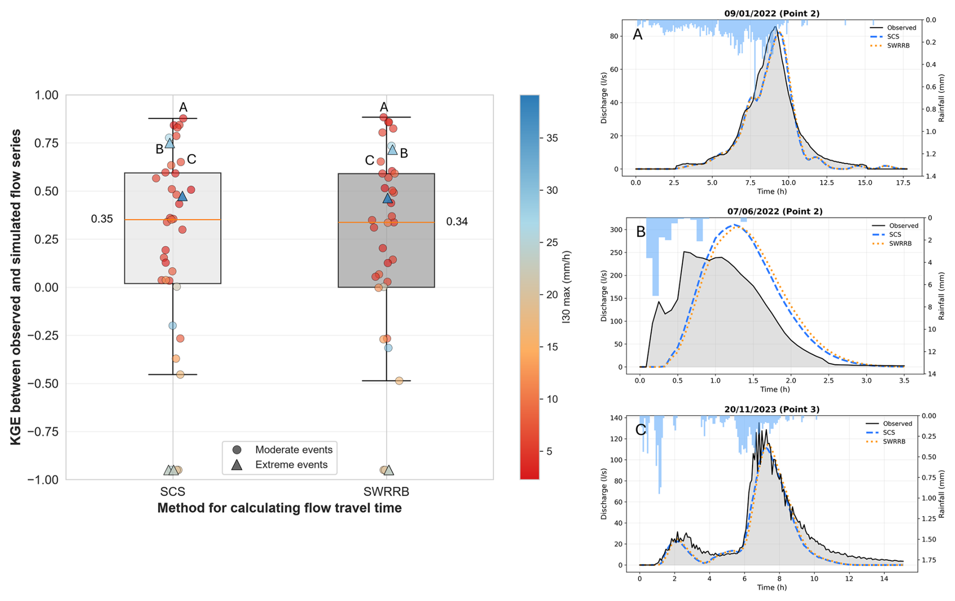
Figure 8 Distribution of KGE between observed and simulated flows by Hidropixel for the SCS and SWRRB methods (left-hand panel). Each dot represents a single rainfall-runoff event (n=39). Marker shapes distinguish event categories (circles for normal events, triangles for extreme events), while the colour gradient indicates the maximum 30 min rainfall intensity. The lower bound of the y-axis is fixed at −1 to avoid displaying extreme negative values. The right-hand panels present representative hydrographs illustrating the model's performance at Point 2 under (A) moderate rainfall conditions (KGE = 0.88) and (B) extreme rainfall conditions (KGE = 0.73), as well as its performance at Point 3 (KGE = 0.65).

A Spearman rank correlation analysis between the efficiency metric (KGE) and key hydro-meteorological descriptors reveals distinctly regime-dependent performance. Model skill exhibits a significant positive correlation with rainfall duration ($\mathit{\rho }={\mathrm{0.40}}^{*}$), but a highly significant negative correlation with maximum rainfall intensity (I30 max, $\mathit{\rho }=-{\mathrm{0.46}}^{**}$). Total rainfall depth shows no significant influence. Consequently, acceptable hydrograph restitution (positive KGE) is primarily achieved during prolonged, lower-intensity rainfall events, whereas severe model failures coincide with short-duration, high-intensity storms. These results again highlight that the static SCS-CN framework, formulated as an event-total runoff equation without an explicit representation of within-storm rainfall intensity, lacks the temporal resolution to capture rapid Hortonian runoff processes.

To further dissect the model's routing behaviour, the relative errors for Q_p, T_p and T_b were analysed for both routing methods. The results confirm the statistical similarity between the SCS and SWRRB methods, with both exhibiting identical error patterns and median values (Fig. 9).

Regarding Q_p, the analysis shows no systematic bias (median relative errors of −7 % to −9 %), but reveals pronounced dispersion (Fig. 9). Extreme events display very large positive deviations, frequently exceeding 100 %, confirming that Q_p errors are heavily dominated by high-intensity storms. However, discharge observations during such high-magnitude floods are inherently subject to substantial uncertainty due to extreme flows reaching the hydraulic and operational limits of the in situ measurement infrastructure. Beyond these observational limits, this volatility is consistent with the mechanical propagation of the volumetric uncertainties discussed in Sect. 3.1, where the production module's threshold behaviour triggers disproportionate peak responses once the abstraction is exceeded (Walega et al., 2020).

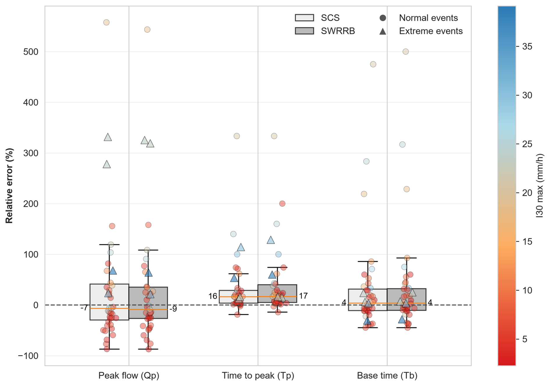
Figure 9 Relative errors (%) of hydrological flood indicators for events (based on Jain's method to estimate runoff volume). The boxes compare Hidropixel SCS and SWRRB for peak discharge (Q_p), time to peak (T_p), and base time (T_b). Marker shapes distinguish event categories (circles for normal events, triangles for extreme events), while the colour gradient indicates the maximum 30 min rainfall intensity. Median values are indicated on each boxplot.

The overwhelming sensitivity of Q_p to CN parameterization compared to routing variables (e.g., T_c) is well-documented (Banasik et al., 2016; Mishra and Singh, 2003; Moghadasi et al., 2018; Ponce and Hawkins, 1996; Vojtek et al., 2019). Rather than undermining the value of distributed routing, this structural sensitivity highlights critical pathways for future research. To fully leverage high-resolution frameworks like Hidropixel, there is a clear need to transition from static CN tables toward dynamic, continuous soil moisture accounting. Integrating satellite-derived antecedent moisture or radar-based infiltration modelling would allow the precision of the 1 m hydraulic routing to be matched by a similarly refined production module, finally overcoming the ”all-or-nothing” threshold behaviour of the classical framework.

A notable finding of this temporal analysis lies in the synchronization of the runoff window. While the model exhibits a consistent delay in time to peak – with median overestimations of +16 % (SCS) and +17 % (SWRRB) plausibly linked to flow-path tortuosity in the 1 m DEM – the base time errors remain centred near zero (4 %). This indicates that, despite the timing offset, the observed and simulated runoff windows coincide reasonably well, suggesting the routing architecture behaves consistently across the tested events rather than erratically. Any observed narrowing or widening of the hydrograph is more likely a secondary consequence of volumetric deviations (Sect. 3.1) than a structural deficiency in transfer timing.

Consequently, the selection between the SCS and SWRRB methods should be guided primarily by the specific modelling objective rather than raw predictive efficiency. The SCS velocity method offers superior spatial discretization, explicitly representing landscape heterogeneity; this makes it particularly effective for assessing the impact of localized land-use features (e.g., specific crop allocations or buffer strips). However, this high resolution renders it inherently susceptible to local DEM artifacts and grid-size dependencies, potentially necessitating targeted spatial calibration. Conversely, the SWRRB approach relies on a simpler, averaged classification of flow regimes. This averaging acts as a spatial low-pass filter, making the method significantly more robust against topographic noise and easier to implement a priori, but at the inevitable cost of smoothing out fine-scale spatial heterogeneity along the flow paths. In essence, the structural strengths of one method mirror the inherent weaknesses of the other.

While this study deliberately focuses on a single, intensively monitored 111 ha catchment to evaluate internal routing mechanics at high resolution, the specific performance metrics derived from its two nested outlets cannot be directly generalized. As demonstrated by Soulis (2018), who observed marked shifts in SCS-CN behaviour following environmental changes, runoff response is highly sensitive to local watershed conditions. Consequently, the relative performance of the routing methods may vary in larger or morphologically contrasting landscapes. Nevertheless, this limitation applies to the empirical validation rather than the model structure itself. As evidenced by the computational stress-tests on larger Walloon catchments (Appendix B), the distributed framework is architecturally scalable, providing a computationally viable foundation for broader regional applications.

3.3 Flood hazard assessment

Building upon the comparative analyses, this final section operationalizes a spatially distributed flood hazard assessment. Based on the efficiency criteria established in Sect. 3.1 and 3.2, the optimal configuration combines the Jain-adjusted CN method with the Hidropixel distributed SCS routing to explicitly account for landscape heterogeneity. By iteratively computing the Q_p for every pixel along the concentrated flow paths, this framework directly translates the hydrological model into a continuous, high-resolution pluvial flood susceptibility map of the drainage network.

Because the main added value claimed for this framework is the spatial identification of critical discharge locations, and not only outlet-scale agreement, the mapped concentrated flow paths were further assessed against independent field and imagery evidence, particularly in the heavily managed northern cultivated part of the catchment (Appendix F). This spatial validation indicates that the main flow paths are topographically robust, while minor pathways in the northern sector show greater inter-annual mobility linked to tillage practices.

3.3.1 Application to an observed rainfall event

To illustrate the spatial consistency and operational potential of the proposed framework, the model is applied to a multi-modal rainfall event (2 January 2024; duration: 18 h, total depth: 28 mm). Figure 10 demonstrates the model's capacity to propagate runoff dynamically throughout the catchment using high-resolution topographic data. An accompanying animation of discharge rates (Supplement, Video S1) further emphasizes the framework's capability for operational risk management. Complementary analyses and further validation examples across diverse rainfall profiles are available in the appendices (Figs. E1 and E2).

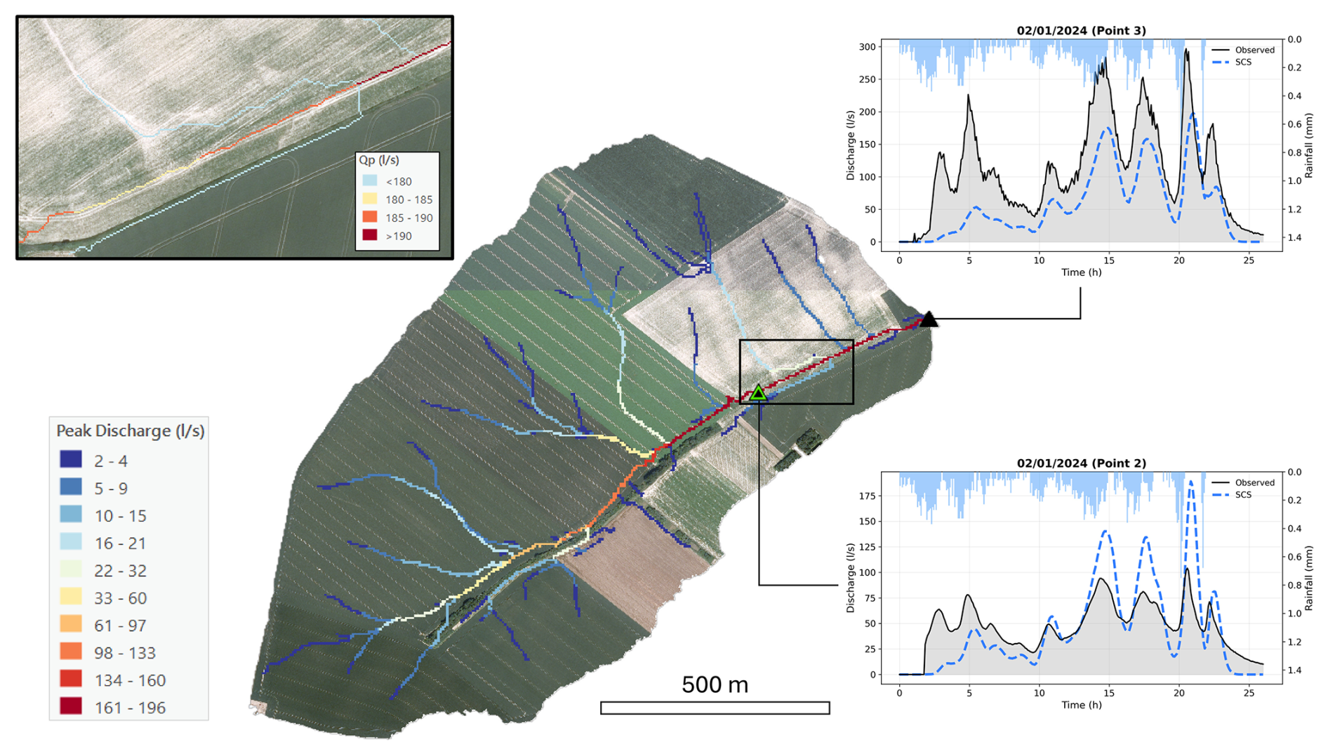
Figure 10 Spatial distribution of simulated Q_p using the SCS velocity method along the concentrated flow paths of the catchment during the 2 January 2024 rainfall event (duration: 18 h, total depth: 28 mm). The right panels display the corresponding hydrographs at the upstream (Point 2) and downstream (Point 3) monitoring stations, comparing observed discharge with the model outputs using both the SCS and SWRRB routing configurations. The zoomed area highlights the spatial variability of Q_p. Maps data: © Service public de Wallonie, 2018.

As highlighted in the magnified inset, the model reproduces two hydrodynamic behaviours that dictate the spatial variability of Q_p. First, on gentle slopes where the contributing area increases slowly, the hydrograph tends to broaden and its peak attenuates. Because low gradients significantly reduce flow velocity, runoff generated across the landscape converges locally over an extended period (Paiva and Lima, 2024; Woltemade and Potter, 1994).

Conversely, where landscape morphology forces flow paths to rapidly converge, local peak amplification occurs. In these areas, lateral runoff inputs arrive simultaneously (in-phase). Because discharge scales non-linearly with the contributing area (power law), this rapid, in-phase superposition of tributary flows yields disproportionately large flood peaks (Ayalew et al., 2014; Bracken and Croke, 2007; Ogden and Dawdy, 2003). This spatial heterogeneity in routing behaviour explains why hydrograph peaks do not always scale monotonically downstream: attenuation dominates over gentle, unconnected reaches, whereas amplification appears where connectivity and drainage area increase.

The accompanying hydrographs at Point 2 and Point 3 confirm the method's ability to reproduce complex, multi-peak catchment responses (Fig. 10). Both the SCS and SWRRB models successfully capture the timing and magnitude of the primary peaks generated by the rainfall bursts later in the event. However, a noticeable discrepancy occurs during the initial hours (3 to 6 h), where the model completely misses the first observed runoff peak. This physically illustrates the structural limitation of the static initial abstraction threshold discussed previously.

Ultimately, this application illustrates the potential of coupling a distributed volumetric approach (adjusted SCS-CN) with high-resolution topographic routing (Hidropixel) in ungauged agricultural areas. The framework provides a spatially explicit, first-order quantification of pluvial flood susceptibility without requiring extensive parameter calibration, though its predictive skill for individual events remains constrained by the runoff-generation module rather than by the routing scheme itself. To further bridge this predictive gap, future evolutions of the tool should address the rigid threshold behaviour of the runoff generation module. Furthermore, coupling these conceptual estimates with machine learning or regionalization in hybrid frameworks offers a promising avenue for transferring hydrological behaviour from gauged to ungauged catchments (Prakash et al., 2025).

3.3.2 Application to extreme design rainfall scenarios

In the absence of observational data for such rare magnitudes, the application to extreme meteorological forcing (25-year and 100-year return period design storms) must be interpreted as an exploratory scenario analysis rather than a validated prediction. Within the limits of a model-structure-driven scenario, it illustrates how the framework could be used to delineate flood-prone corridors and to explore how flow propagation might accelerate under exceptional rainfall in ungauged agricultural catchments.

By applying Meyersohn's equation (Eq. 14) to adjust pixel-level travel times according to extreme rainfall intensities, the model produces a drastic shift in the spatial distribution of travel times (Fig. 11). During a standard 2-year event, the maximum travel time reaches 78 min, whereas it decreases to 46 and 37 min under the 25-year and 100-year scenarios, respectively. This simulated reduction is conceptually consistent with the expected physical hydrological behaviour of extreme events, where greater runoff volumes generate deeper flows that significantly increase hydraulic efficiency and flow velocities.

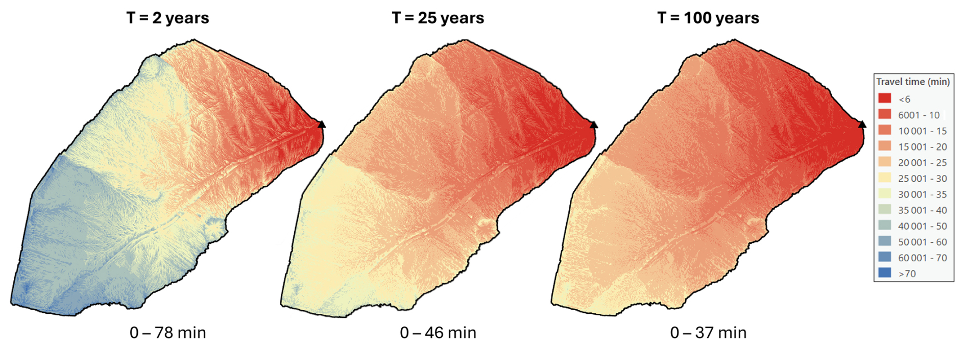
Figure 11 Spatial distribution of runoff travel times across the catchment under varying design storm magnitudes (2-year, 25-year, and 100-year return periods) adjusted according to Meyersohn's formula.

A spatial comparison of simulated Q_p between the 25-year and 100-year design storms reveals a pronounced amplification of flow magnitude along the main concentrated flow path (Fig. 12). While Q_p increases substantially – nearly doubling at the main outlet from approximately 1826 L s⁻¹ (T=25 years) to 3514  L s⁻¹ (T=100 years) – this relative amplification is highly spatially heterogeneous. The percentage increase in Q_p systematically escalates as flow paths converge, rising from moderate values in the headwaters (30 % to 50 %) to a maximum exceeding 90 % in the main thalweg. Within this modelled scenario, this localized intensification suggests that flood severity under extreme forcing would be primarily driven by enhanced routing efficiency and the rapid, non-linear synchronization of upstream contributions, a pattern generated by the assumed model structure and travel-time adjustment.

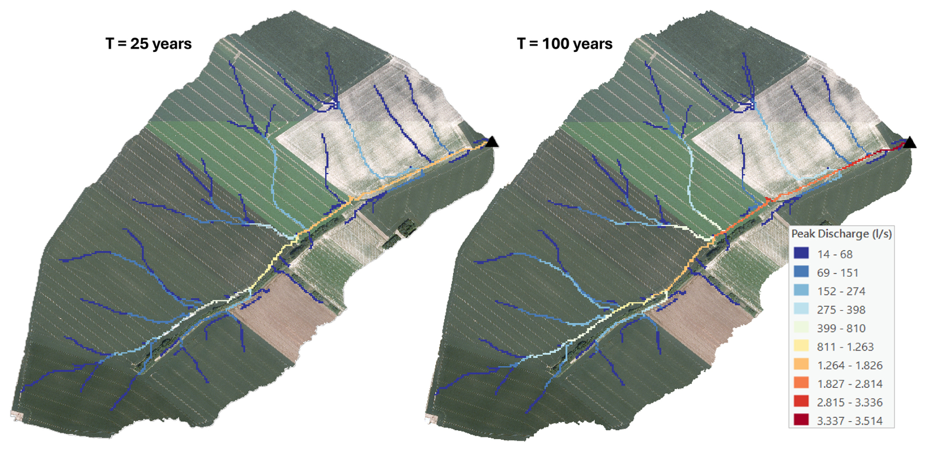
Figure 12 Spatial distribution of simulated Q_p along concentrated flow paths for the 25-year and 100-year design storms. Maps data: © Service public de Wallonie, 2018.

Characterizing flood hazard solely through the spatial distribution of Q_p presents inherent limitations, as it omits the explicit temporal dynamics of the flood wave (e.g., rate of rise, duration of inundation). However, Q_p remains a highly pertinent primary indicator for ungauged catchments (Blöschl, 2013; Prakash et al., 2025). Because Q_p mathematically integrates both the total volume of excess runoff and the geomorphological convergence of flow paths, it effectively captures the maximum hydraulic stress exerted on the landscape and infrastructure.

4 Summary and conclusions

This study evaluated a high-resolution, spatially distributed hydrological framework designed to assess pluvial flood hazards in ungauged agricultural catchments. By systematically decoupling the runoff generation and routing phases, the analysis clarified both the capabilities and the structural limits of parsimonious conceptual modelling in ungauged environments, providing a transparent basis for targeted future improvement.

The foundation of this framework rests on an accurate estimation of effective runoff. Adopting the Jain method for initial abstraction markedly reduced volumetric bias relative to the traditional SCS-CN approach, but this did not remove a deeper structural issue: because the static CN framework has no mechanism for representing within-storm intensity, its skill degrades specifically for short, high-intensity events, where infiltration-excess (Hortonian) runoff dominates the response. Moving past this ceiling will likely require future conceptual frameworks to shift from static, event-based thresholds toward continuous soil-moisture accounting.

Regarding hydraulic transfer, the model reproduced the duration of the observed runoff window, with base-time errors centred near zero despite a systematic delay in time to peak (+16 % to +17 %) and the sensitivity of peak magnitude to upstream inputs. The comparative analysis further showed only marginal differences in overall restitution between the velocity-based (SCS) and path-averaged (SWRRB) routing schemes, indicating that the routing behaviour is consistent regardless of the specific method chosen, rather than that the routing stage actively corrects volumetric errors. Extending the analysis from the single outlet to the full drainage network at 1 m resolution further showed the model reproducing the interplay between hydrodynamic attenuation along low-gradient reaches and the non-linear convergence of flows at tributary junctions, an internally coherent, though not independently validated, spatial behaviour that supports the framework's suitability for spatially distributed applications.

These spatially distributed results illustrate one valuable use of the framework for proactive risk evaluation: complementing single-outlet predictions with a spatially continuous, fine-scale characterization of peak discharge across the whole drainage network, a capability that lumped models cannot offer. Applied to 25-year and 100-year design storms, the framework shows the active flow network implied by the model structure expanding markedly, with modelled peak discharges escalating by over 90 % along the main thalweg under the assumed travel-time adjustment for extreme events. As this scenario is generated by the model structure rather than independently observed, it should be regarded as an illustrative, exploratory outcome; even so, it demonstrates the kind of spatial differentiation this framework can offer to help identify locations most susceptible to extreme flows.

The primary limitation of this work is that it has so far been evaluated on a single, though intensively monitored, hydrological system: the two nested outlets (84 and 111 ha) are dependent evaluation points rather than genuinely independent, contrasting catchments, so the relative performance of the tested methods cannot yet be generalized to different climates, soils, topographies, or catchment sizes. This is a limitation of the available validation data rather than of the model structure itself: the framework's parsimony, together with the computational scalability already demonstrated on larger Walloon catchments, points to strong potential for broader deployment, pending confirmation of its predictive performance and, where warranted, local calibration across contrasting environments. Extending this evaluation to additional catchments is accordingly a natural next step toward establishing this framework as an operational tool for pluvial flood risk evaluation in ungauged agricultural landscapes, alongside a continued commitment to expanded field monitoring and open data sharing.

Appendix A: Travel time and resolution sensitivity

Figure A1 illustrates the sensitivity of spatially distributed local flow velocities to DEM resolution. At high resolutions, a larger proportion of the catchment is characterized by sheet flow, resulting in lower local velocities. Conversely, coarser resolutions tend to artificially accelerate flow concentration, significantly reducing the frequency of sheet flow pixels. This highlights the necessity of implementing a minimum slope threshold to prevent local travel times from reaching physically unrealistic values in nearly flat terrain. The 0.5 % threshold retained for this study yields T_c estimates consistent in order of magnitude with both the Mockus (1961) lag equation and direct hydrograph observations (Sect. 2.5.3); its physical basis (observed thalweg slopes) is detailed below.

Table A1 extends this analysis to the full modelling chain, comparing hydrological performance across four grid resolutions (1, 2, 5, and 10 m) for the 39 observed events using the SCS transfer method. Coarsening the grid smooths the topography and artificially accelerates flow routing, producing a severe overestimation of Q_p at 5 and 10 m; a 2 m grid moderately degrades hydrograph shape performance relative to 1 m but reduces computational cost, and may be a reasonable operational compromise for wider regional applications.

Figures A2 and A3 further show the joint sensitivity of T_c to the imposed minimum slope threshold and grid resolution for the 111 ha and 84 ha catchments, respectively. Across both catchments, a minimum slope of 0.3 to 5 % yields T_c values consistent with field observations and the Mockus (1961) lag-time relationship; the 0.005 m m⁻¹ threshold retained in Sect. 2.3.2 was selected to remain consistent with observed thalweg slopes rather than to optimize timing metrics.

Table A1 Hydrological performance metrics across spatial resolutions for the SCS transfer method (39 events; T_c: time of concentration, T_p: time to peak, Q_p: peak discharge, V: runoff volume).

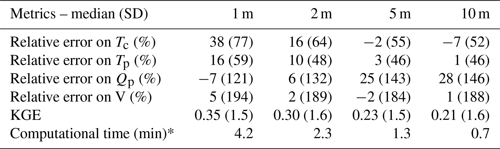
* Workstation with 32 GB RAM and a 4-core CPU.

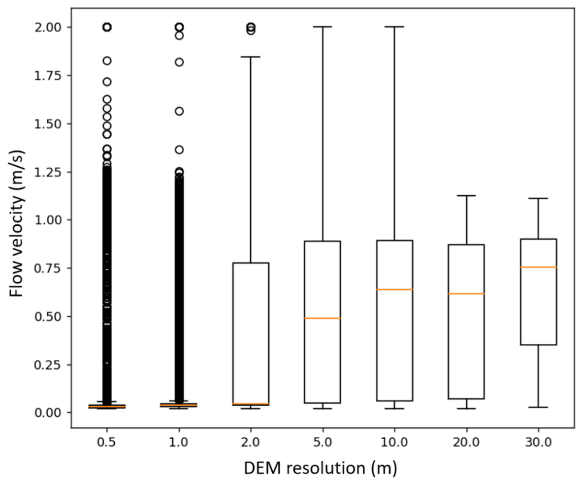
Figure A1 Impact of spatial resolution on local water velocity estimates calculated via the SCS velocity method in the 84 ha catchment. Orange lines represent median values for each resolution.

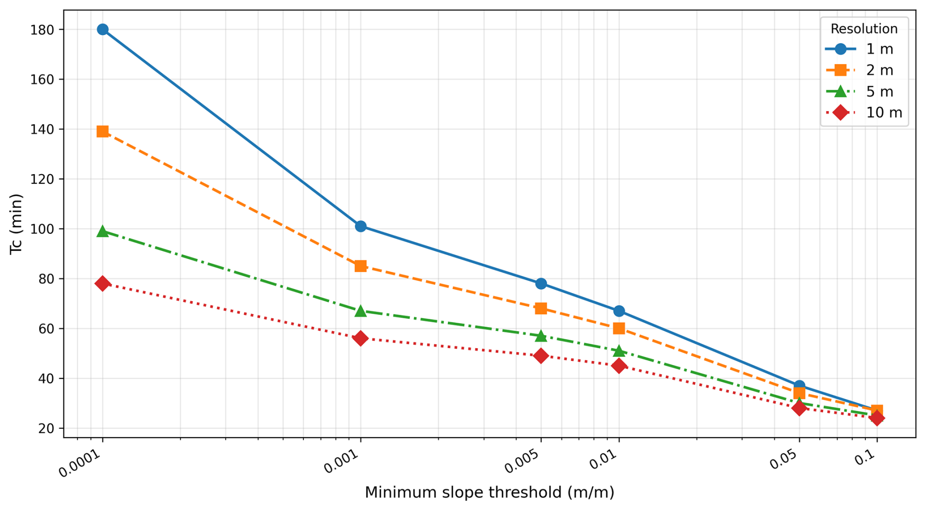
Figure A2 Sensitivity of time of concentration to minimum slope threshold and resolution in the 111 ha catchment.

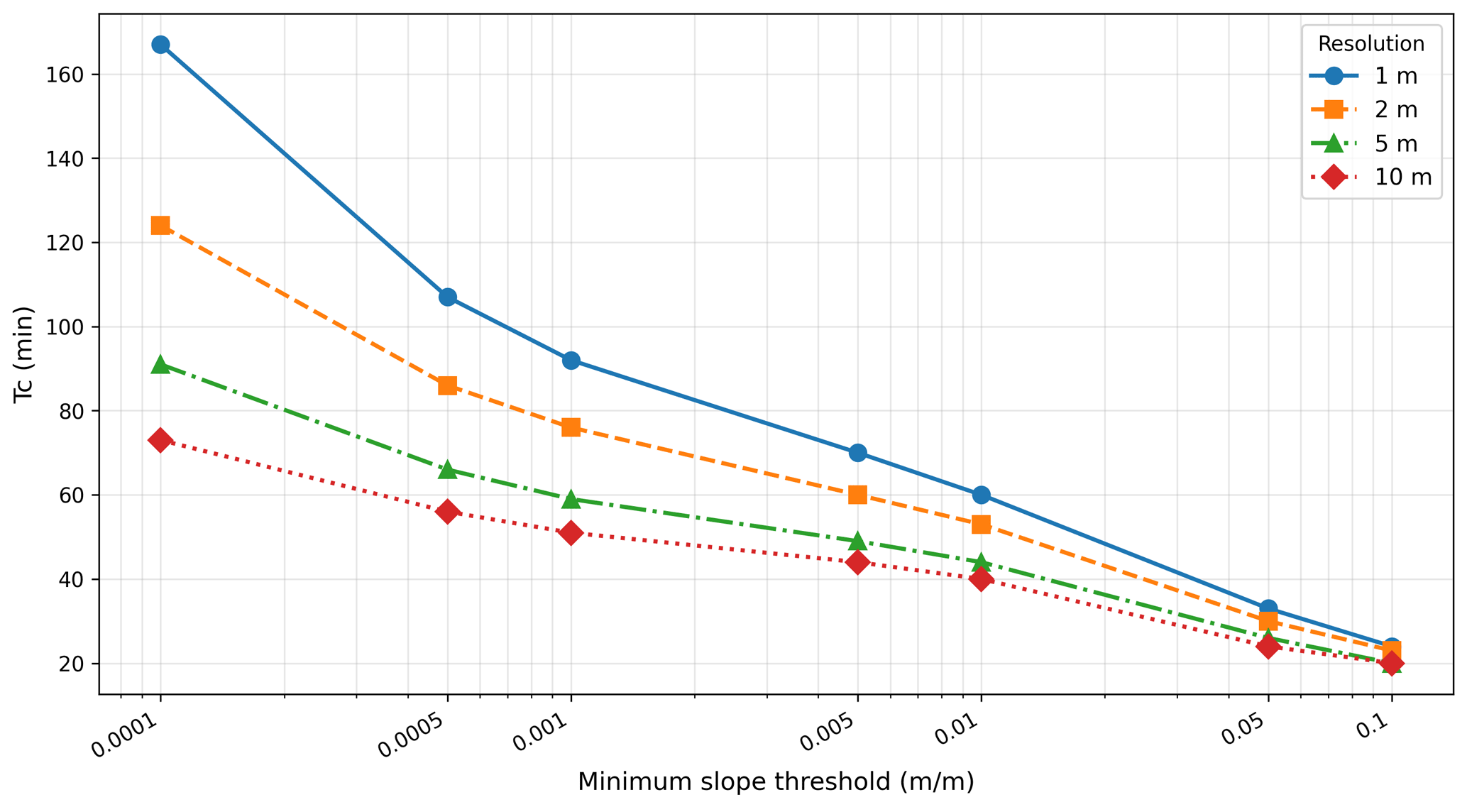
Figure A3 Sensitivity of time of concentration to minimum slope threshold and resolution in the 84 ha catchment.

Appendix B: Computational optimization

This appendix provides the detailed benchmarks supporting the computational-optimization results summarized in Sect. 2.3.5. At the Chastre catchment, the 1.4 min of preprocessing and 2.8 min of processing reported for the 39 events at the two outlets break down into raster/grid setup and per-event convolution, respectively; for the spatialized application, the grouping procedure compresses ∼ 1 065 000 pixel-level (CN, T_v) pairs into ∼ 550 pairs. Table B1 details the calculation times for the four larger AQUALIM catchments introduced in Sect. 2.3.5, and Fig. B1 maps their location. The most demanding test concerned the distributed application along concentrated flow paths in the catchment at Flobecq, with a fine drainage threshold of 0.5 ha: the 115 650 temporary outlets (about 13 times more than at Chastre, on a grid with about 13.5 times more active cells) required 198 min for a single storm.

Table B1 Characteristics of catchments within the AQUALIM network and calculation times for applying Hidropixel to the outlet. LHP = Longest Hydraulic Path; RHW length = total length of the Walloon hydrographic network within the catchment.

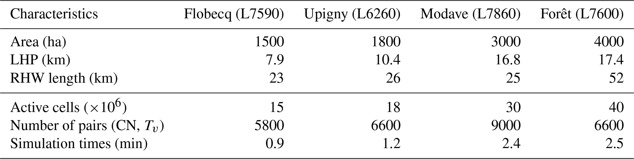
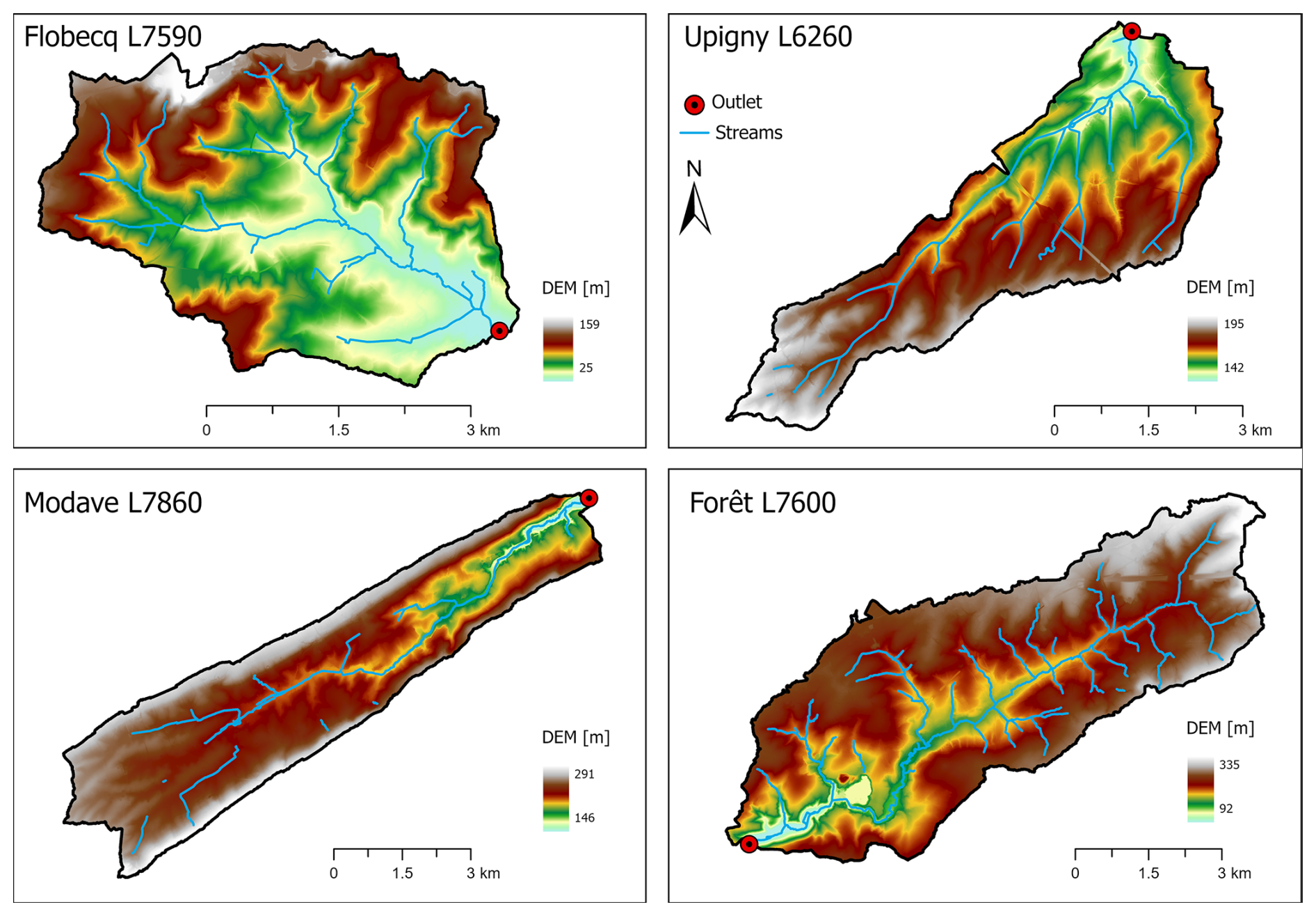
Figure B1 Location of the AQUALIM catchments used for the computational benchmark, including watercourses, topography and outlets.

Appendix C: Hydrological data

Table C1 Characteristics of selected rainfall-runoff events for the Chastre catchment (Points 2 and 3).

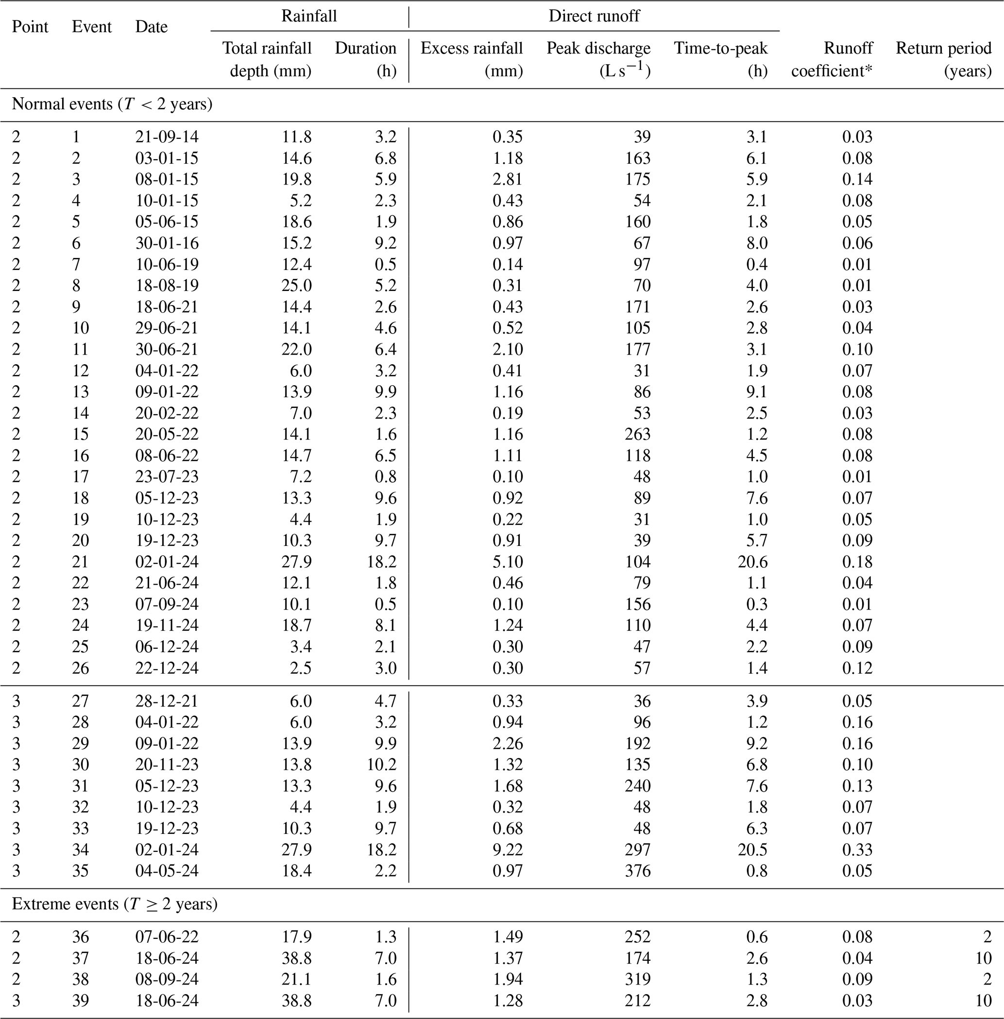
* runoff coefficient = excess rainfall/rainfall.

Appendix D: Runoff estimation

Van Oost (2003) proposes an adjusted Curve Number (CN) of each grid cell of the drainage area, computing it as a function of crop development and soil crusting stages:

$$\begin{array}{}\text{(D1)}& {\mathrm{CN}}_{\mathrm{adj}}={\mathrm{CN}}_{\max }-\left({\displaystyle \frac{C_{\mathrm{c}}}{\mathrm{100}}}\times c_{\mathrm{1}}\right)+\left({\displaystyle \frac{C_{\mathrm{r}}}{\mathrm{4}}}\times c_{\mathrm{2}}\right)\end{array}$$

where CN_max represents the maximum theoretical CN derived from the USDA-SCS handbook for specific combinations of cover types and hydrological soil groups typical of Walloon agricultural practices; C_c is the fractional crop cover (%); C_r denotes the soil crusting stage and c₁ and c₂ are coefficients.

Subsequently, Maugnard (2015) established an empirical relationship via linear regression, demonstrating a significant correlation between the optimal initial abstraction ratio (λ), total rainfall depth (P), and the CN (R²=0.76, NSE = 0.77, RMSE = 0.025, n=17):

$$\begin{array}{}\text{(D2)}& \mathit{\lambda }=-\mathrm{0.01527}-\mathrm{0.04806}\times P+\mathrm{0.0007609}\times P\times \mathrm{CN}\end{array}$$

To evaluate these dynamic approaches, the Van Oost method for dynamic CN adjustment was coupled with the Jain method for I_a estimation. As illustrated in Fig. D1, the Van Oost approach does not improve the estimation of runoff volumes. It introduces a systematic overestimation (median relative errors of +33 % and +36 %). Conversely, the Maugnard method – which relies on a locally calibrated linear regression to adjust λ – demonstrates an improvement, yielding predictions much closer to the observed volumes. These results underscore that refining the parameter λ through context-specific empirical regressions is a more robust and effective strategy for capturing runoff generation than modifying the core CN parameter itself.

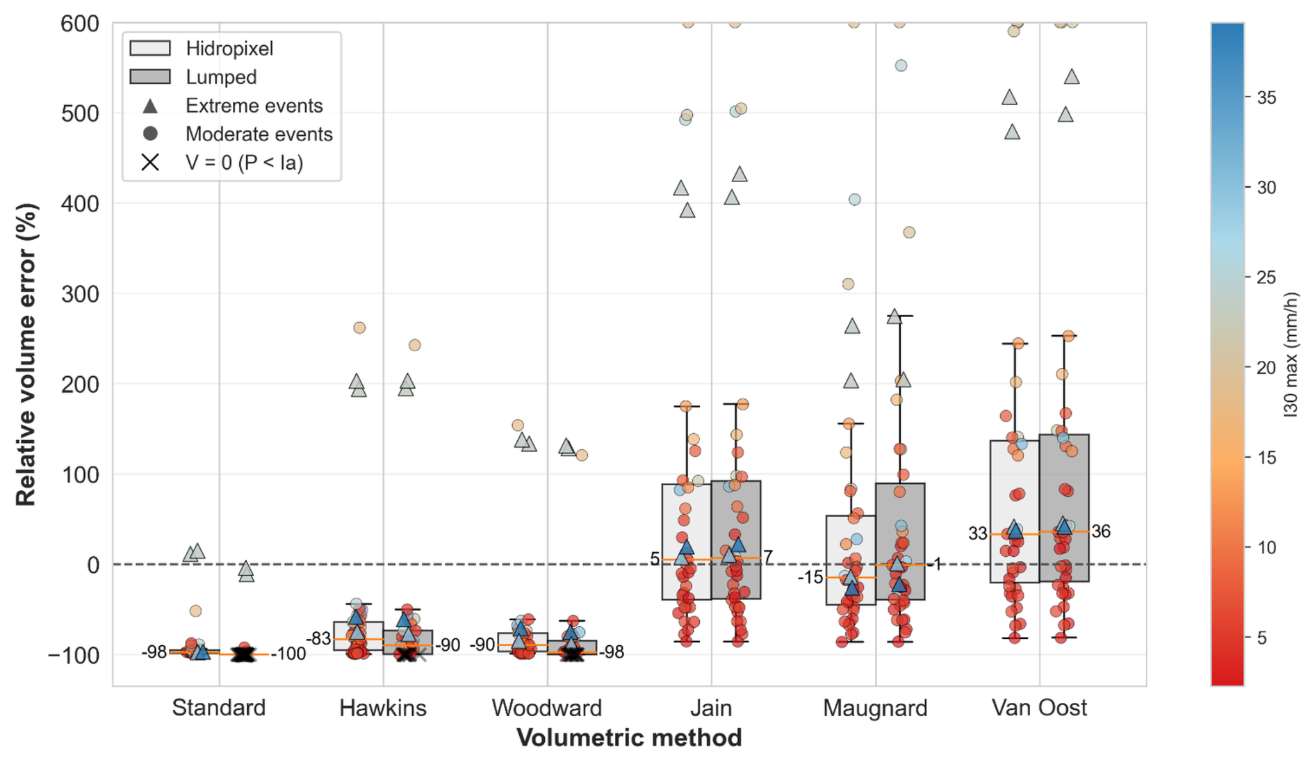
Figure D1 Comparative boxplots of signed relative volume error (%) for runoff events (n=39) at the Chastre watershed for the four SCS-CN formulations of Fig. 4 and the two locally adjusted approaches described in this appendix (Maugnard: event-dependent λ, Eq. D2; Van Oost: dynamic CN, Eq. D1, combined with the Jain initial abstraction), using the Hidropixel model (light grey) and a lumped model approach (grey). Marker shapes distinguish event categories (circles for normal events, triangles for extreme events), while the colour gradient indicates the I30 max (the maximum intensity of rainfall recorded over a period of 30 min), and the black crosses highlight zero-runoff simulations (P < I_a). Numeric median values are displayed.

Appendix E: Hydrograph estimation

Figure E1 Comparison of observed and simulated hydrographs for a selection of distinct rainfall-runoff events recorded between 2014 and 2024.

Figure E2 Simultaneous hydrograph restitution at the upstream (Point 2) and downstream (Point 3) monitoring stations for two rainfall events.

Appendix F: Pluvial flood susceptibility map

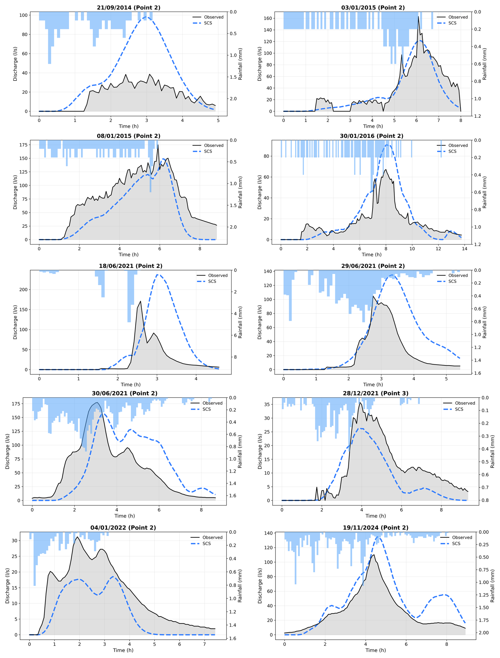
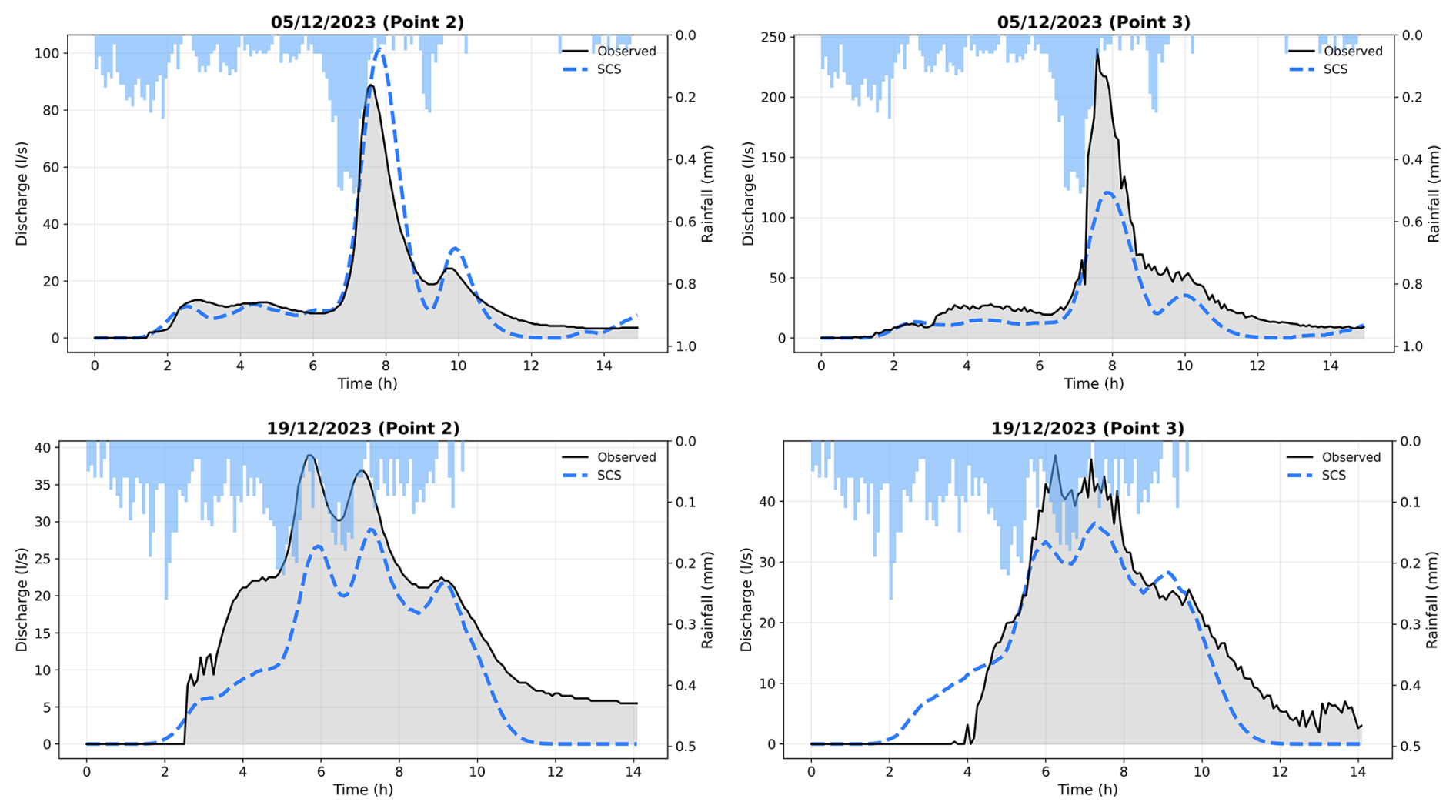
Because the main added value claimed for the pluvial flood susceptibility map is the spatial identification of critical discharge locations, and not only outlet-scale agreement, the reliability of the mapped concentrated flow paths was further assessed against field and imagery evidence, particularly in the heavily managed northern cultivated part of the catchment (Fig. F2). Figure  F3 maps the spatial dispersion of simulated flow paths as an uncertainty layer, highlighting greater variability of minor pathways in this northern sector, consistent with the mobility of secondary routes linked to tillage practices. Figure F4 compares simulated concentrated flow networks at four resolutions against 12 ephemeral gullies observed after an intense storm on 29 May 2026: the 1 m and 2 m resolutions align more closely with the observed gullies than the 5 m and 10 m resolutions, providing independent support for the retained grid size in addition to the analysis in Appendix A.

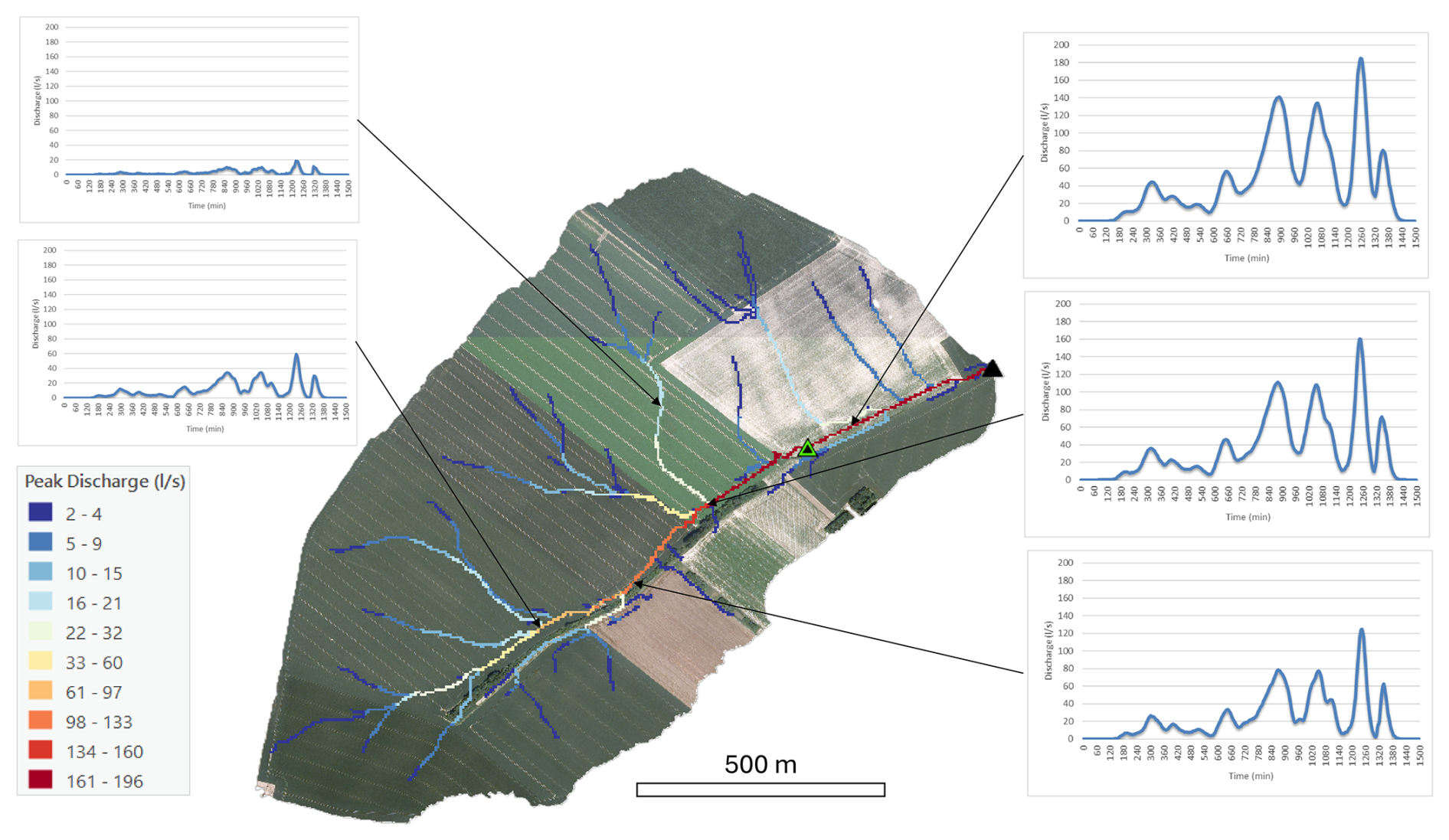
Figure F1 Spatio-temporal simulation of the 2 January 2024 runoff event using the Hidropixel SCS model. The central map displays peak discharges (L s⁻¹) along concentrated flow paths, while the surrounding panels show simulated hydrographs at specific locations. The black triangle denotes the main outlet, and the green triangle indicates an upstream gauging station. Maps data: © Service public de Wallonie, 2018.

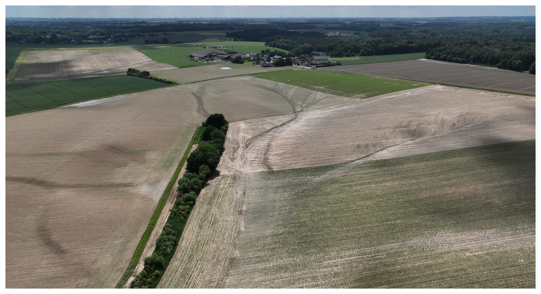
Figure F2 Aerial view of the Chastre headwater catchment following an intense storm on 29 May 2026. Photograph: Gilles Swerts.

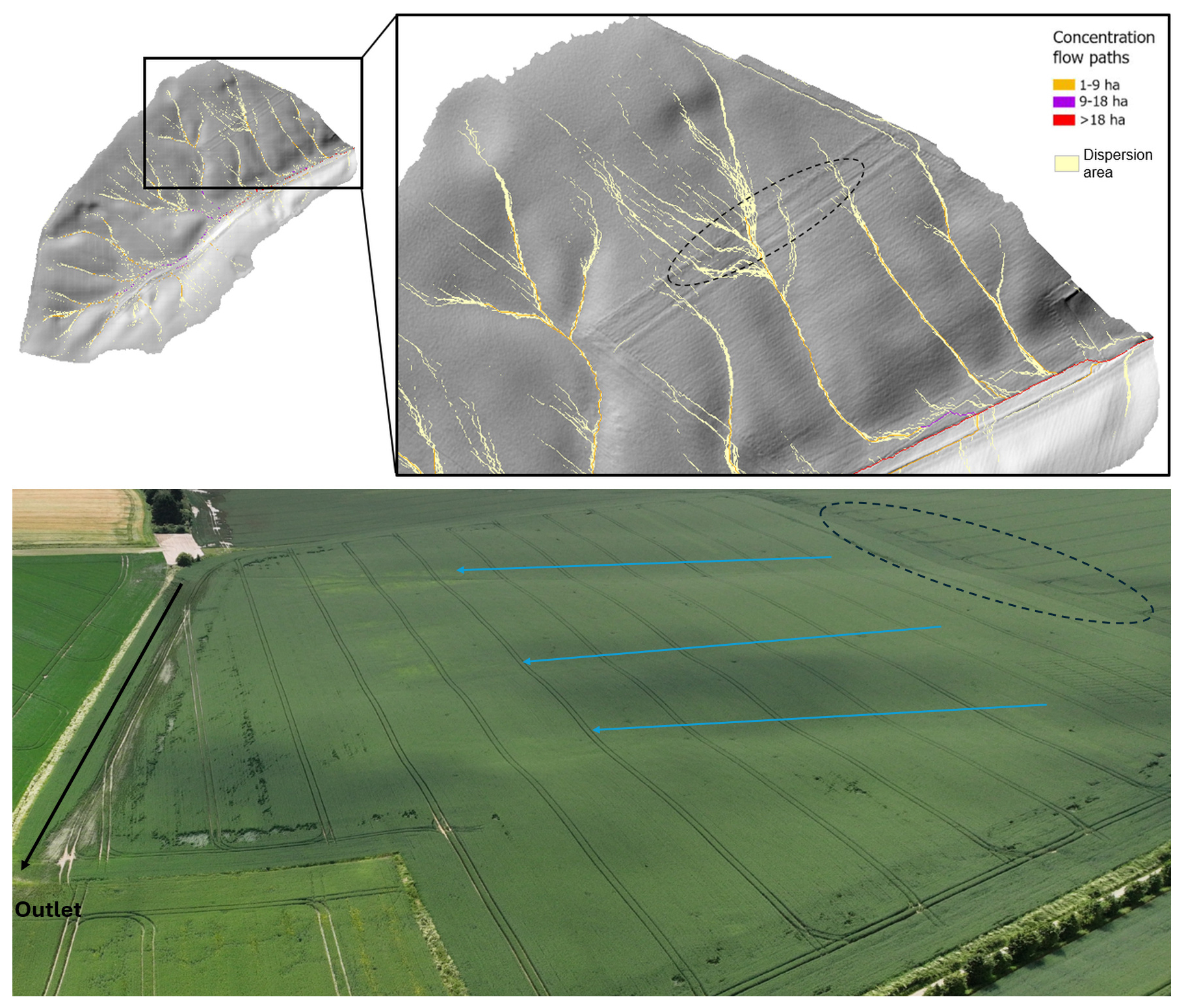
Figure F3 Top: spatial dispersion and mapped location of simulated flow paths. Bottom: aerial view of the northern hillslope of the Chastre catchment following the 29 May 2026 storm, highlighting the three main concentrated flow axes (blue) converging into the primary thalweg (black); flow paths within the dotted area exhibit a diffuse and mobile pattern. Aerial photograph: Gilles Swerts.

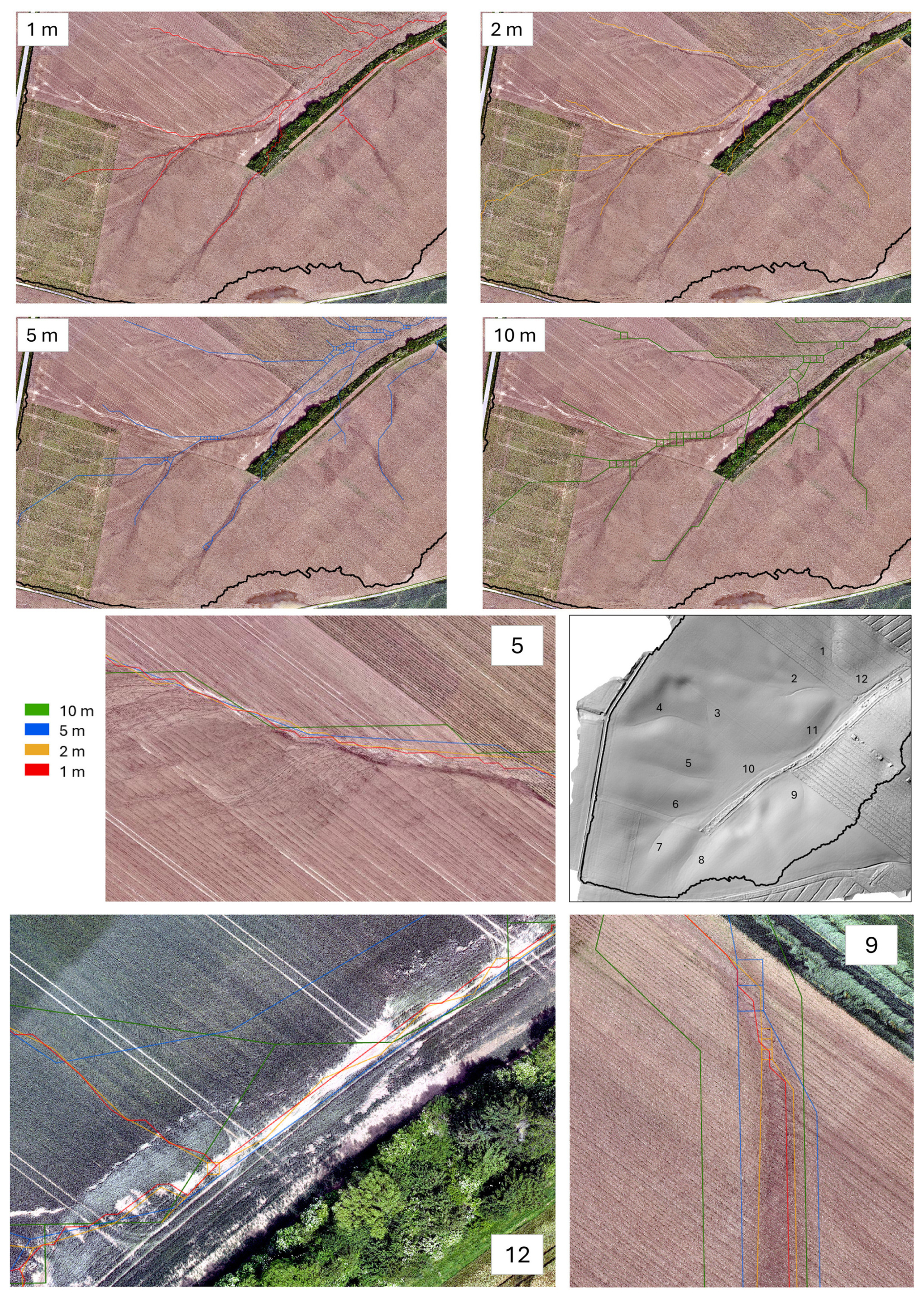
Figure F4 Simulated concentrated flow networks extracted at four spatial resolutions (1, 2, 5, and 10 m) based on the 2021–2022 DEM, with the location of 12 ephemeral gullies observed after the 29 May 2026 storm, mapped on the post-event DEM (captured 30 May 2026).