Enhancing hydrological representation of the Brahmaputra basin through terrestrial water storage and surface soil moisture Data Assimilation

Understanding the dynamics of terrestrial water storage (TWS), and its components such as surface soil moisture (SSM) and groundwater, is important for the Brahmaputra River basin, where water resources are expected to experience increasing demand and are highly vulnerable to extreme hydrological events and climate change. However, water storage dynamics are complex and difficult to capture by state-of-the-art large-scale hydrological models. In this study, we implement a multi-variate daily TWS and daily SSM sequential Data Assimilation (DA) to integrate the satellite observations in the World Wide Water Resources Assessment model (W3RA) with the aim of improving model-derived water storage dynamics. In our methodology, we propose a model space covariance localization approach that is compared with three other approaches used in the previous literature. The results show that this new approach is the only one to effectively reduce cross-variable influences along the vertical water storage profile, which have been reported as one of the main challenges of multi-variate land DA. A validation of the multi-variate DA estimates (for the period 2004–2015) indicates that more realistic decadal trend and inter-annual variability are introduced into the TWS and groundwater estimates, increasing the correlation coefficients with the Standardized Precipitation Evapotranspiration Index and observed groundwater levels by +0.24 to +0.54 correlation points. With respect to SSM, DA induces a general phase shift, especially around mountain areas. Improved land water storage estimates reveal a land water decline of 70.9 GT per decade for the period 2004–2015 in the Brahmaputra River basin, which constitutes approximately half of the TWS decline in that period, with the other half caused by glacier retreat (67.5 GT per decade).

1 Introduction

Due to population growth and urban and industrial development, as well as climate change, water availability and security in the Brahmaputra River basin are becoming more uncertain (Das and Kumar, 2019). On the one hand, demographic and economic growth, accompanied by consequent changes in land use, can lead to a higher water demand, potentially resulting in regional water scarcity (Gain and Wada, 2014; Kirby and Mainuddin, 2022). Groundwater depletion has already been detected related to agricultural and urban water use (for example, in northwestern Bangladesh, a region adjacent to the Brahmaputra basin, or around the city of Dhaka in the southern part of the Brahmaputra basin) (Shamsudduha et al., 2012, computed over period 1985–2007). On the other hand, the IPCC report (IPCC, 2023) states that climate change, through changes in precipitation patterns (Gogoi et al., 2023), glacier melting and snow melting (Lutz et al., 2014; Nie et al., 2021), is likely to cause increased extreme river flows in the Brahmaputra River, further enhancing flooding events (Gain et al., 2011; Masood et al., 2015; Dutta et al., 2021; Alam et al., 2021). In addition, sea-level rise also poses higher flood risks for coastal areas (Brown et al., 2018; Rahman et al., 2019). These events can cause enormous human and economic damage and threaten the water security of the region (Das and Kumar, 2019; Kirby and Mainuddin, 2022).

Effective management of water resources and mitigation of risks posed by extreme events require a clear understanding of spatial and temporal changes in the variability of land water storage (that is, groundwater and soil water). This knowledge is essential to plan and implement water conservation measures, especially in the face of climate change (Sammonds et al., 2021). Hydrological models are the main tool to simulate and predict water variability; however, their performance is limited due to many factors such as the complexity of hydrological processes, limited in situ data for performing calibrations, and the uncertainty of input climate forcing fields (Kauffeldt et al., 2016; Mehrnegar et al., 2020).

Satellite Earth Observations (EO) can be used to monitor various aspects of the global water cycle (Dube et al., 2023) and are especially useful in poorly gauged or ungauged basins. Measurements provided by the Gravity Recovery and Climate Experiment (GRACE, Tapley et al., 2004) and its Follow-On mission (GRACE-FO, Flechtner et al., 2014) can be used to detect time-variable changes in terrestrial water storage (TWS), which represent the total amount of water on Earth's land surface and in the subsurface, encompassing components such as groundwater, soil moisture, lakes, rivers, snowpack, and glaciers. Changes in TWS reflect the net effect of natural processes and anthropogenic modifications on the available water budget (Eicker et al., 2016; Kusche et al., 2016). Remotely sensed surface soil moisture (SSM) is an important EO product, which represents the water stored in the first few centimeters of the Earth's surface (Kerr et al., 2010; Entekhabi et al., 2010). Satellite missions such as SMOS, SMAP, Sentinel-1, and MetOp have been used in the past to retrieve SSM products globally.

Although satellite-based observations provide very useful information, their performance is limited to low spatial-temporal resolutions: for example, GRACE-FO is resolved monthly with ∼ 300 km resolution or daily with ∼ 450 km resolution, while SSM can be few-daily with 1–25 km spatial resolution. Additionally, temporal gaps can be found in the data series due to sensor or orbital instability (mainly in TWS), as well as difficult retrieval conditions (in SSM), and uncertainties in retrieval algorithms may cause biases (Gruber et al., 2020; Yang et al., 2024). Furthermore, each EO product only provides information on a particular variable of the water cycle while, in contrast, models simulate various water storage and flux components, as well as their interactions. Hence, a logical step is to integrate EOs into models to combine their advantages, which can be pursued through data-model fusion frameworks.

The ensemble-based sequential Data Assimilation (DA) is a popular approach to perform data-model fusion in hydrological applications (Reichle, 2008). These DA frameworks allow us to integrate various observations, when they are available, within the model while accounting for the uncertainty of both the model and the observations. The assimilation of monthly GRACE TWS in hydrological models has been applied globally (Li et al., 2019; Gerdener et al., 2023; Yang et al., 2025) and within various river basins. The TWS DA has been found to improve the TWS and groundwater dynamics of models, by correcting trend, seasonal, and inter-annual variability (Zaitchik et al., 2008; van Dijk et al., 2014; Girotto et al., 2016, 2017; Schumacher et al., 2018; Getirana et al., 2020; Schumacher et al., 2025). Generally speaking, the product of TWS DA presents the realism of GRACE(-FO) TWS observations while preserving the finer spatial resolution and individual water storage and flux estimates of hydrological models (Yang et al., 2025) and allows to compute the water storage variability of individual water storage components with a better accuracy than simpler component reduction methods (Getirana et al., 2025). However, one of the main challenges reported in the TWS DA is the vertical disaggregation of storage updates, which can degrade SSM estimates (Girotto et al., 2016, 2019; Tangdamrongsub et al., 2020; Retegui-Schiettekatte et al., 2025a).

Various studies have also assimilated SSM retrievals into different hydrological models (e.g., Reichle and Koster, 2005; Crow and Ryu, 2009; Brocca et al., 2010; Renzullo et al., 2014; Ridler et al., 2014; Massari et al., 2015; Blyverket et al., 2019; De Lannoy et al., 2024). Some of them reported notable improvements in near-surface soil moisture and root-zone water storage estimations, as well as a better representation of hydrological fluxes such as runoff (Brocca et al., 2010; Massari et al., 2015; De Lannoy et al., 2024). Nevertheless, SSM DA has also been found to (partially) degrade deeper soil water, groundwater and TWS estimates (Ridler et al., 2014; Tian et al., 2017; Girotto et al., 2019) and have a neutral or negative impact on river runoff estimates (Chen et al., 2011; Matgen et al., 2012; Ridler et al., 2014).

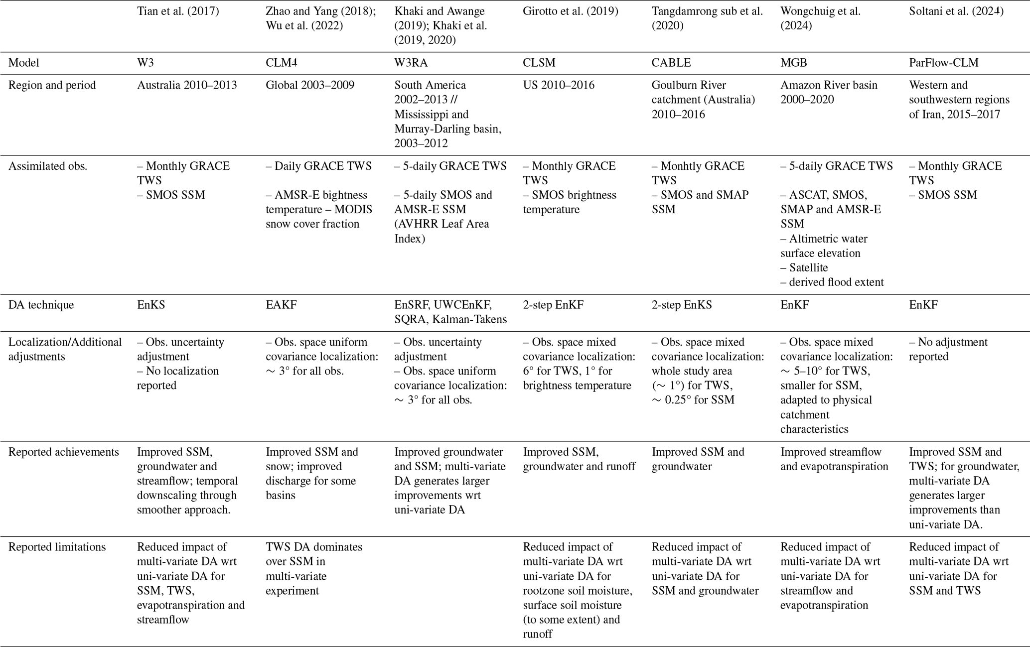
A strategy to address the complementary issues of TWS DA and SSM DA can be realized by simultaneously assimilating both observations (multi-variate DA). Table 1 provides an overview of the existing literature on multi-variate TWS and SSM DA and their DA techniques, as well as their main findings. These multi-variate experiments were found to improve both SSM and groundwater components (Tian et al., 2017; Girotto et al., 2019; Khaki et al., 2019; Khaki and Awange, 2019; Khaki et al., 2020; Tangdamrongsub et al., 2020; Soltani et al., 2024) and indirectly modify other water balance components such as snow, streamflow, and evapotranspiration (Zhao and Yang, 2018; Wu et al., 2022; Wongchuig et al., 2024).

Nevertheless, the multi-variate DA still presents challenges that remain unsolved. Namely, previous studies reported conflicts between TWS and SSM observations that, to different extents, diminish the improvement of model estimates in the multi-variate implementation compared to a uni-variate implementation (Tian et al., 2017; Zhao and Yang, 2018; Girotto et al., 2019; Tangdamrongsub et al., 2020; Wongchuig et al., 2024; Soltani et al., 2024). This cross-variable interference is not necessarily a problem and has been found to lead to enhanced estimates in some cases (Khaki et al., 2019; Khaki and Awange, 2019; Khaki et al., 2020; Soltani et al., 2024). However, conflicts between datasets can appear in regions with the presence of irrigation, as is the case of the Brahmaputra River basin, where negative TWS and groundwater trends caused by water pumping can be strongly anti-correlated with increasing SSM values caused by expanding irrigation practices (Goswami et al., 2024). If the influence of TWS DA in the SSM component is not adequately constrained, this can result in the introduction of long term trends in SSM and evapotranspiration, degrading the representation of these variables within the model (Girotto et al., 2017). In multi-variate DA scenarios, Girotto et al. (2019) showed that when the updates introduced by the different observations are anti-correlated, they can end up canceling each other. Furthermore, in some of these studies, the success of the DA experiment is found to be conditioned by an appropriate adjustment of observation uncertainties, which should be estimated heuristically (Tian et al., 2017).

Discrepancies in previous results likely stem from differences in experimental settings such as the study area, observation sampling rate or methodology. One of the methodological aspects in which previous studies diverge is the implementation of covariance localization. Covariance localization is widely used in hydrological DA, as well as in other geoscientific disciplines, to mitigate spurious ensemble correlations or sampling errors arising from limited ensemble sizes and inherent constraints in ensemble perturbation methods. Especially, distance-based localization helps to confine the influence of observations to relevant spatial domains, thereby increasing their impact on the relevant model variables (Houtekamer and Mitchell, 1998; Hamill et al., 2001). Various ways exist to implement such localization and, so far, there have been no studies assessing the impact of localization choices on multi-variate TWS and SSM DA experiments.

In this study, satellite-derived TWS and SSM are assimilated into the World Wide Water Resources Assessment model (W3RA) in the Brahmaputra River basin. The study pursues two main objectives: (i) to explore how different multi-variate TWS and SSM DA settings can generate or avoid some of the issues reported in previous literature, and (ii) to produce improved land water storage estimates for the Brahmaputra River basin. Especially, we aim to improve model water storage estimates in the sub-seasonal to decadal timescale, with the aim of supporting future investigations concerning the water storage variability and availability (in the inter-annual to decadal timescale) as well as the role of land water in flood generation mechanisms (in sub-seasonal to inter-annual timescale). To reach the first objective, we test and compare different covariance localization settings used in previous literature and propose a novel approach, here called “model space mixed localization”, to maximize the performance of the multi-variate DA. Regarding the second objective, we first validate the multi-variate DA estimates against independent in situ streamflow and groundwater data, as well as the Standardized Precipitation Evapotranspiration Index (SPEI) and SSM estimates from an independent model. Finally, we analyze the decadal, inter-annual and seasonal variability of land water storage in the region.

The paper is organized as follows: first, the study area, data and model, method and experimental setting are introduced; second, evaluation and and interpretation of the results are presented and discussed; finally, concluding remarks close the paper.

Table 1 Summary of experimental setting and main result of previous multi-variate land DA experiments involving TWS and SSM data. “wrt” = with respect to; “obs” = observation(s). The abbreviations in “DA techniques” (row 4) refer to the Ensemble Kalman Filter (EnKF), Ensemble Kalman Smoother (EnKS), Ensemble Adjustment Kalman Filter (EAKF), Ensemble Square Root Filter (EnSRF), Unsupervised Weak Constrained Ensemble Kalman Filter (UWCEnKF) and Square Root Analysis (SQRA). More details on localization and DA adjustment approaches (row 5) is provided in Sect. 2.3.3.

2 Study area, data and method

2.1 Study area

The Brahmaputra River basin, one of the largest river basins in the world, has a drainage area of about 530 000 km² (which covers China, India, Bangladesh, and Bhutan). The hydrology of the basin is characterized by a strong seasonality caused by monsoonal precipitation, with a wet season from June to September accounting for 60 % to 70 % of its annual rainfall (Immerzeel, 2008). This results in a rapid saturation of the soil around June, which is typically sustained during the wet period. Groundwater also presents a strong seasonality as it is largely recharged through rainfall and river flow infiltration processes in the monsoon season (Medhi et al., 2024; Shamsudduha et al., 2022).

The Brahmaputra River produces an average discharge of approximately 20 000 m³ s⁻¹. In the upper stage of the river, glacier and snow melt are estimated to contribute approximately 20 %–25 % of river discharge, while rainfall runoff dominates with 59 % of contribution (Lutz et al., 2014; Chen et al., 2017). Floods are common during the wet season in southern agricultural floodplains and often cause huge socio-economical impacts, including large fatalities, the displacement of thousands of people, and damage to crops resulting in famine (Brammer, 1990; Mirza, 2003). The river flow regime is expected to change with climate change: glaciers in the area have been reported to retreat by approximately −0.5 m of water equivalent per year for the period 2000–2018/2019 (Shean et al., 2020; Hugonnet et al., 2021; Vishwakarma et al., 2022), and are likely to further retreat in the next few decades (Lutz et al., 2014; Nie et al., 2021). This is expected to generate higher flows during the monsoon period, increasing the risk of flooding and posing a threat to the livelihoods and food and water security of the area (IPCC, 2023; Uhe et al., 2019; Dutta et al., 2021; Alam et al., 2021).

The communities along the Brahmaputra River basin depend on these water resources for agriculture and domestic use. Approximately 25 % of the Brahmaputra River Basin is classified as agricultural land (Commission, 2014), with a particularly high presence of irrigation in Bangladesh (Siebert et al., 2013). Although surface water is abundant during the monsoon season, it can become scarce during the dry season, increasing the need for groundwater abstraction for agricultural irrigation (Shamsudduha and Panda, 2019). Estimates for October 2013 suggest that the groundwater-fed irrigation exceeds surface water-fed irrigation in many parts of the basin (Siebert et al., 2013). Groundwater storage declines of −2 to −5 cm per year due to agricultural abstraction have been reported in the northwest of Bangladesh (region adjacent to the Brahmaputra River basin). In addition, similar-sized declines in groundwater have also been reported around the capital city of Bangladesh, Dhaka (Shamsudduha et al., 2012). In the rest of the basin (that is, the East and West sub-basins of this study), the anthropogenic impact on land water resources is considered limited (Khandu et al., 2016; Maina et al., 2024).

The Brahmaputra River basin was selected as a study area for two reasons: (i) we sought to evaluate multi-variate data assimilation techniques in a hydrological environment that differs substantially from those examined in previous studies (e.g., Australia or the US, see Table 1); and (ii) the basin exhibits a pronounced hydrological variability which is difficult to track precisely due to the lack of abundant in situ observations, leading to significant challenges for water resources management and hydrological risk mitigation. As such, this region stands to benefit from refined and more accurate hydrological water storage estimates. Despite the limited availability of ground-based hydrological observations in the region, we were able to collect in situ groundwater and river water level measurements for portions of the basin. These datasets provide a foundation for validating a subset of our model outputs.

In addition to the Brahmaputra River basin, the DA area in this study also includes the Meghna River basin (drainage area of approximately 82 000 km²) as well as the confluence of the Brahmaputra, Ganges, and Meghna Rivers. As the two latter only contribute in the South sub-basin (Fig. 1), and for the sake of conciseness, in this study the whole area is generically referred to as the Brahmaputra River basin. For the assimilation of TWS and interpretation of the results, the basin was divided into the East, West and South sub-basins (Fig. 1), with areas of 100 000–250 000 km² chosen to be consistent with the approximate daily GRACE TWS resolution. Therefore, the reduced resolution of daily observations is not expected to be an issue at sub-basin scale.

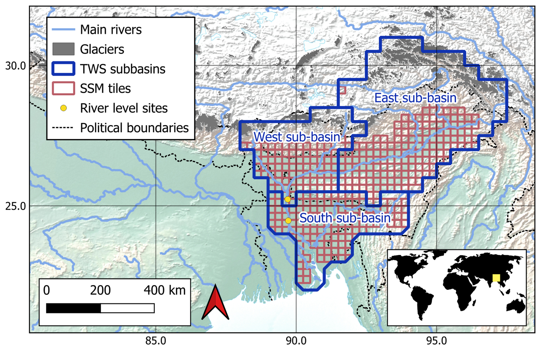
Figure 1 An overview of the Brahmaputra River basin with the three sub-basins, in which TWS is assimilated (blue boundaries, areas of 253 000, 105 000, and 107 000 km²). The red grid boxes (0.25°×0.25°) represent the locations where the ESA CCI SSM product is assimilated.

2.2 Data and model

2.2.1 Model

This study uses the World Wide Water Resources Assessment model (W3RA, van Dijk, 2010; van Dijk et al., 2013). Previous studies suggest that W3RA offers a good performance at representing water storage variability when compared to other state-of-the-art models (Schellekens et al., 2017; Mehrnegar et al., 2020). The evaluations performed in this study also suggest a reasonable agreement between the model and satellite observations prior to DA in terms of water storage (see Sect. 4.1), suggesting that W3RA provides a reasonable representation of the large-scale water storage variability in the Brahmaputra River basin and constitutes an appropriate baseline for the DA experiments. In addition, as a parsimonious model, W3RA presents low computational requirements and is therefore well suited to reduce the computational expense of the experiments.

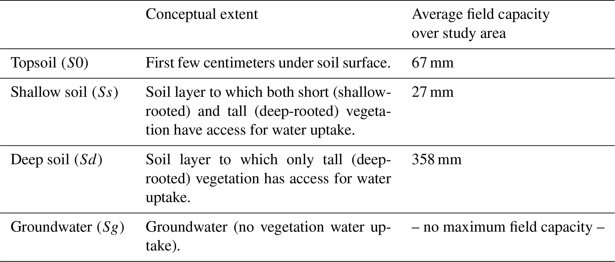
The W3RA model represents natural land water and energy exchange processes. The soil profile is divided into four layers: topsoil, shallow soil, deep soil, and groundwater (Table 2). In this study, topsoil and shallow soil are treated jointly as “SSM”, and deep soil and groundwater are treated jointly as “groundwater” (a detailed explanation of the reason behind this aggregation is provided in Sect. 3.1). Water exchange processes within the soil are described through the representation of infiltration, drainage, root water uptake, and capillary rise. Soil and surface water evaporation is computed as a linear function of available energy, and groundwater discharge is estimated through a linear reservoir model (van Dijk, 2010; van Dijk et al., 2013). Heterogeneities in soil composition are not considered, and anthropogenic water use activities, such as groundwater pumping or agricultural irrigation, are not modeled.

Vegetation is modeled in two categories, shallow-rooted short vegetation (grass and shrubs) and deep-rooted tall vegetation (trees), which are represented as two different Hydrological Response Units (HRUs). The proportion of vegetation belonging to each category for each grid cell is determined through the satellite-based tree cover fraction map by Hansen et al. (2003). Vegetation transpiration is computed as the minimum of maximum root water uptake and optimum transpiration rate, where the latter is estimated using the Penman-Monteith equation. Root water uptake is modeled through a linear ramp function (as a function of soil water content) (van Dijk, 2010; van Dijk et al., 2013). Differences in crop types or seasonal variations of vegetation are not considered. More details on the explicit formulation of all these processes can be found in van Dijk (2010); van Dijk et al. (2013).

W3RA also has a snow module that represents snow accumulation and melt based on a degree day approach (van Dijk et al., 2013). Glaciers are not represented within the snow module. To compute surface water routing, a grid-based model was coupled with W3RA where each grid cell is represented as a linear reservoir (Mizukami et al., 2016). Lakes, reservoirs and floodplanes are not represented within the routing model, and evaporation of water routed in streams and rivers is not represented either.

The model parameterization for the Brahmaputra River basin was performed through a regionalization approach (van Dijk et al., 2013). No further calibration or correction of forcing data was implemented since possible errors resulting from these limitations are expected to be addressed through the DA process. A prior calibration of the model against streamflow would be unlikely to modify the main conclusions of this study due to the little sensitivity of streamflow estimates to water storage dynamics (later analyzed in Sect. 4.3.4).

The model was run with a spatial resolution of 0.1°×0.1° (approximately 10 km×10 km) and a daily temporal resolution, and was forced with precipitation, maximum and minimum temperature, and downward surface solar radiation data derived from ERA5 (Hersbach and Dee, 2016) and ERA5-Land (Munoz Sabater, 2019) (see more details in Sect. 3.1).

Table 2 Overview of W3RA land water storage components and their respective field capacities in the study area.

2.2.2 Assimilated data

The daily TWS was derived from the daily GRACE products of ITSG-2018 (Mayer-Gürr et al., 2018; Kvas et al., 2019). The daily product was chosen over traditional monthly GRACE products for two reasons: (i) to avoid the temporal mismatch between TWS and SSM observations, as well as with the model; and (ii) to improve the model TWS estimates on the sub-seasonal and sub-monthly timescales (Retegui-Schiettekatte et al., 2025a). In this study, we only considered data for the period 2003–2015 to limit the temporal extent of each experiment (and hence their computational cost) and to avoid having to deal with the gap between GRACE and GRACE-FO missions (2017–2018). The post-processing applied to the data included recommended spherical harmonic corrections, geophysical inversion, and leakage error correction (see more details in Retegui-Schiettekatte et al., 2025a; Mehrnegar and Forootan, 2025). The time-dependent error variance of the spherical harmonics was post-processed accordingly and rescaled at the end of the process to fit the values reported in Boergens et al. (2022). It should be mentioned that the Kalman Smoother approach used to generate the daily TWS product can be expected to introduce temporal autocorrelations in the daily to weekly timescale. In the present study, these temporal correlations were not accounted for because (i) the temporal autocorrelation is expected to be weaker in the seasonal to inter-annual timescale considered in this study; and (ii) the magnitude or temporal structure of these autocorrelations have not been quantified yet, and computing them would require a whole dedicated study. Accounting for temporal autocorrelations could be relevant for future studies exploring water storage estimates in weekly to sub-weekly timescales.

The daily SSM estimates originate from the European Space Agency Climate Change Initiative (ESA CCI) Combined SSM product (v08.1) (Gruber et al., 2019; Dorigo et al., 2017; Preimesberger et al., 2021). This dataset was chosen because of its daily sampling, avoiding a temporal mismatch with the model. The combined product merges SSM retrievals derived from various active and passive satellite sensors and is provided on 0.25°×0.25° tiles (Fig. 1), with uncertainties computed using a triple-collocation technique. The merging process includes rescaling the retrievals to a common baseline (modeled soil moisture of GLDAS Noah, Gruber et al., 2019). To avoid mismatches with our model, before performing DA, we re-rescaled the ESA CCI SSM estimates to the range of W3RA SSM estimates (see more details in Sect. 3.1).

2.2.3 Validation data

In situ groundwater level observations and river water level observations of the Bangladesh Water Development Board (BWDB) (see Shamsudduha et al., 2012, 2022), available in the area of Bangladesh, have been used for validation. 263 groundwater observation sites were available for the study area, located mainly in the South sub-basin and covering the entire study period (Fig. 8). The groundwater level data have been quality controlled by the BWDB and curated by Shamsudduha et al. (2022). Specific yield information was originally obtained from around 200 pumping tests and interpolated using ground lithology maps by Shamsudduha et al. (2011).

Regarding river level observation sites, a selection was carried out according to the following criteria: (i) the sites should be located on the main branch of the Brahmaputra River; and (ii) they should be as close as possible to the sub-basin outlets, to reflect the impact of sub-basin averaged TWS assimilation on river water levels. Two sites were selected for the West and South sub-basins (Fig. 1), which provide data for the entire study period with few temporal gaps (Fig. 10). No river observation site was available for the East sub-basin.

The Standardized Precipitation Evapotranspiration Index (SPEI, Vicente-Serrano et al., 2010) is an indicator of hydrological dryness-wetness conditions, and in this study it was used to perform a consistency-check with TWS estimates. Although the SPEI reflects variability of net water fluxes rather than water storage, previous literature suggests that the aggregation of SPEI over time windows of 12 months or longer effectively works as a temporal integration, leading to higher correlations with TWS (Zhang et al., 2018; Cammalleri et al., 2019; Satish Kumar et al., 2021). Based on this literature, the SPEI-12 was chosen for comparisons in this study. The SPEI-12 time series for each sub-basin were derived from the Global Drought Monitor (Beguería et al., 2014) and are used to validate the inter-annual groundwater dynamics.

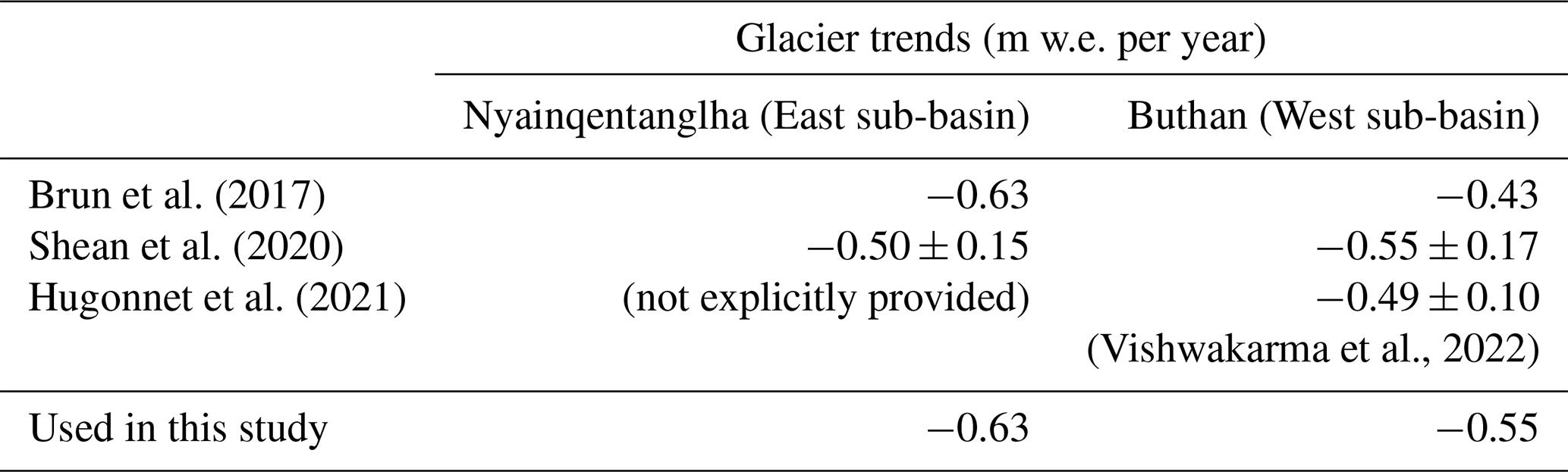
TWS in the East and West sub-basins is affected by trends caused by glacier retreat (Wouters et al., 2019; Li et al., 2023; Sherpa and Werth, 2025). These glacier trends have been quantified in previous literature using satellite stereo imagery (Brun et al., 2017; Shean et al., 2020; Hugonnet et al., 2021). In this study, previously computed glacier trends were used to reduce the glacier impact from TWS in Sect. 4.4, allowing to compare the mass loss caused by glacier retreat with that caused by other hydrological processes. The Randolph Glacier Inventory 7.0 dataset (RGI Consortium, 2023) was used to compute the total area covered by glaciers in each sub-basin, resulting in 7719 and 3406 km² for the East and West sub-basins, respectively.

An independent validation of SSM is not straightforward because (i) there is no in situ SSM observation openly available in the study region; and (ii) various active and passive satellite SSM retrievals are included in the assimilated ESA CCI Combined SSM, and therefore a comparison against any of these SSM products cannot be considered independent. Due to these limitations, SSM estimates are evaluated against soil water storage estimates from the WaterGAP global hydrology and water use model (Döll et al., 2003; Müller Schmied et al., 2024; Nyenah et al., 2025), which are resolved with daily and 0.5°×0.5° resolution. A 10 km resolution topographic slope dataset was used to support the interpretation of spatial SSM difference patterns (Amatulli et al., 2018).

2.3 Method

2.3.1 Data Assimilation

Following previous literature on land DA (Girotto et al., 2019; Tangdamrongsub et al., 2022; Wongchuig et al., 2024), DA was performed using an Ensemble Kalman Filter (EnKF) approach (Evensen, 1994; Houtekamer and Mitchell, 1998; Evensen, 2003). The EnKF is a Monte-Carlo approach in which the uncertainty of the model is computed through an ensemble run of N_e perturbed model realization (more details on the perturbation method can be found in Sect. 3.1). The objective here is to update the ensemble of model states $({\mathbf{X}}_k=[{\mathit{x}}_k^{\left(\mathrm{1}\right)},{\mathit{x}}_k^{\left(\mathrm{2}\right)},\mathrm{\dots },{\mathit{x}}_k^{\left(N_{\mathrm{e}}\right)}\left]\right)$ for every timestep k, where the model state ${\mathit{x}}_k^{\left(i\right)}$ represents the water storage values predicted by the model for each grid cell and each water storage component in that timestep (see a list of these components in Sect. 3.1). The updated model state for the timestep k is computed as

$$\begin{array}{}\text{(1)}& {\mathbf{X}}_k^{+}={\mathbf{X}}_k^{-}+{\mathbf{K}}_k({\mathbf{Y}}_k^{\mathrm{o}}-{\mathbf{HX}}_k^{-}),\end{array}$$

where ${\mathbf{X}}_k^{-}$ is the predicted model state ensemble matrix for the timestep k, which contains, in its column i, the model state of the ith ensemble member, and ${\mathbf{X}}_k^{+}$ is the updated model state ensemble matrix for the same timestep, with a similar structure. The observation matrix ${\mathbf{Y}}_k^{\mathrm{o}}$ contains each ith perturbed set of observation (here TWS, SSM or both) in its ith column. These observations are perturbed according to their uncertainty, in order to guaranty a realistic ensemble spread in the updated model states (Burgers et al., 1998, see more information on the perturbation method in Sect. 3.1). The matrix H is the forward observation operator that, when applied to the model state, generates the observation prediction. K_k is the Kalman gain matrix, which is defined as

$$\begin{array}{}\text{(2)}& {\mathbf{K}}_k=\mathbf{C}\left({\mathbf{X}}_k^{-}\right){\mathbf{H}}^{\top }\left(\mathbf{HC}\right({\mathbf{X}}_k^{-}){\mathbf{H}}^{\top }+{\mathbf{\Sigma }}_{{\mathit{y}}^{\mathrm{o},k}}{)}^{-\mathrm{1}}.\end{array}$$

${\mathbf{\Sigma }}_{{\mathit{y}}^{\mathrm{o}},k}$ refers to the error covariance matrix of the observations. $\mathbf{C}\left({\mathbf{X}}_k^{-}\right)$ is the ensemble-based error covariance matrix of the model state and is computed as $\mathbf{C}\left({\mathbf{X}}_k\right)=\frac{\mathrm{1}}{N_{\mathrm{e}}-\mathrm{1}}\mathrm{\Delta }{\mathbf{X}}_k\mathrm{\Delta }{\mathbf{X}}_k^{\top }$, where the matrix ΔX_k contains, in its ith column, the deviation of the ensemble member i from the ensemble-average of the model state, ${\mathit{x}}_k^{\left(i\right)}-\frac{\mathrm{1}}{N_{\mathrm{e}}}{\sum }_{i=\mathrm{1}}^{N_{\mathrm{e}}}{\mathit{x}}_k^{\left(i\right)}$.

2.3.2 Uni-variate and multi-variate DA

In the uni-variate (i.e., single-observation) TWS DA experiment ${\mathbf{Y}}_{k,\mathrm{TWS}}^{\mathrm{0}}$ and ${\mathbf{\Sigma }}_{{\mathit{y}}_{\mathrm{TWS}}^{\mathrm{o}},k}$ are used within the EnKF equations, which represent the perturbed TWS observations and their uncertainty, respectively. The forward TWS computation operator, H_TWS, vertically aggregates all water storage components and horizontally averages gridded model estimates on three sub-basins (Fig. 1). For the uni-variate SSM DA experiment, ${\mathbf{Y}}_{k,\mathrm{SSM}}^{\mathrm{0}}$ and ${\mathbf{\Sigma }}_{{\mathit{y}}_{\mathrm{SSM}}^{\mathrm{o}},k}$ represent the perturbed SSM observations and their uncertainty, respectively. The forward SSM computation operator (H_SSM) aggregates the water storage components corresponding to SSM and averages gridded model estimates on the 0.25° × 0.25° ESA CCI tiles (Fig. 1).

Multi-variate DA can be implemented in a similar way to uni-variate DA by extending the observation matrix to include all observations in the following way (Wongchuig et al., 2024)

$$\begin{array}{}\text{(3)}& {\mathbf{Y}}_{k,\text{multi-variate}}^{\mathrm{o}}=\left(\begin{array}{l}{\mathbf{Y}}_{k,\mathrm{TWS}}^{\mathrm{o}}\\ {\mathbf{Y}}_{k,\mathrm{SSM}}^{\mathrm{o}}\end{array}\right).\end{array}$$

The observation error covariance matrix and the forward operator matrix also need to be updated accordingly, that is, ${\mathbf{\Sigma }}_{{\mathit{y}}_{\text{multi-variate}}^{\mathrm{o}},k}=\left(\begin{array}{cc}{\mathbf{\Sigma }}_{{\mathit{y}}_{\mathrm{TWS}}^{\mathrm{o}},k}& \mathrm{0}\\ \mathrm{0}& {\mathbf{\Sigma }}_{{\mathit{y}}_{\mathrm{SSM}}^{\mathrm{o}},k}\end{array}\right)$ and ${\mathbf{H}}_{\text{multi-variate}}=\left(\begin{array}{c}{\mathbf{H}}_{\mathrm{TWS}}\\ {\mathbf{H}}_{\mathrm{SSM}}\end{array}\right)$. Note that the matrix ${\mathbf{\Sigma }}_{{\mathit{y}}_{\mathrm{multi}-\mathrm{variate}}^{\mathrm{o}},k}$ represents the empirical observation errors of the GRACE TWS observations and satellite-derived SSM observations. Such empirical errors arise from factors including, but not limited to, instrumental noise, GRACE orbit determination uncertainties, and post-processing errors. Given the fundamentally different measurement principles and processing chains underlying TWS and SSM products, it is theoretically unlikely that correlated empirical observation errors would exist between the two, and it is therefore realistic to set the extra-block-diagonal elements in ${\mathbf{\Sigma }}_{{\mathit{y}}_{\mathrm{multi}-\mathrm{variate}}^{\mathrm{o}},k}$ to zero.

Previous studies by Tian et al. (2017), Girotto et al. (2019), Tangdamrongsub et al. (2020) include two-step update schemes or temporal smoothers to address the temporal mismatch issue between the model and observations. These approaches are not necessary in this study, as both observations are assimilated in the same daily timescale as the model. This implies that the forward observation operator matrices ${\mathbf{H}}_{\mathrm{TWS}/\mathrm{SSM}/\mathrm{multi}-\mathrm{variate}}$ here perform a vertical aggregation and horizontal averaging, but do not apply any temporal averaging.

2.3.3 DA tuning approaches

Most of the previous TWS and SSM DA experiments share a similar EnKF update framework, but tune the DA implementation differently (see Table 1). In this paper, we study the impact of two of these tuning approaches: uncertainty adjustment and covariance localization.

2.3.4 Uncertainty adjustment

The uncertainty adjustment (see, e.g., Tian et al., 2017) is implemented to achieve a better balance between the TWS and SSM observations, and to avoid that one observation type dominates over the other. It consists of multiplying the TWS and SSM observation uncertainties with scaling factors (α_TWS and α_SSM, respectively), which must be set heuristically (see more details in Sect. 3.1),

$$\begin{array}{}\text{(4)}& {\mathbf{\Sigma }}_{{\mathit{y}}_{\text{multi-variate}}^{\mathrm{o}},k}^{\mathrm{adjusted}}=\left(\begin{array}{ll}({\mathit{\alpha }}_{\mathrm{TWS}}{)}^{\mathrm{2}}\cdot {\mathbf{\Sigma }}_{\mathrm{TWS},k}& \mathrm{0}\\ \mathrm{0}& ({\mathit{\alpha }}_{\mathrm{SSM}}{)}^{\mathrm{2}}\cdot {\mathbf{\Sigma }}_{\mathrm{SSM},k}\end{array}\right).\end{array}$$

The optimal value of the factors might differ depending on the value of the uncertainties and the amount of each type of observation that is assimilated (Tian et al., 2017).

2.3.5 Observation space covariance localization

The covariance localization approach is typically used in the field of DA to mitigate the impact of spurious long-range correlations in model ensemble statistics, which can negatively affect the DA update, especially when small ensemble sizes are used (Houtekamer and Mitchell, 1998; Hamill et al., 2001). In short, the approach consists of damping correlations that are above a defined radius that represents the expected correlation range.

Previous studies by Zhao and Yang (2018); Khaki and Awange (2019); Girotto et al. (2019); Tangdamrongsub et al. (2022); Wongchuig et al. (2024) implement observation space covariance localization, where correlations between model variables and observations are damped based on the distance between them. This type of localization ensures that each model variable is influenced only by nearby observations that could realistically affect them (Fig. 2b).

The localization can be discrete (i.e., all observations further than a cutoff radius should be ignored, Houtekamer and Mitchell, 1998) or smooth (i.e., the observations are weighted depending on their distance to each model grid cell, Houtekamer and Mitchell, 2001). Domain localization or local analysis (Mitchell and Houtekamer, 2000; Evensen, 2003) can also be seen as a type of discrete observation space covariance localization. Smooth observation space localization matrices are typically built based on compactly supported distant-dependent functions, such as Gaspari-Cohn functions (Gaspari and Cohn, 1999). The localization matrix $\left({\mathit{\rho }}_{\mathrm{1}/\mathrm{2}}\right)$ is then applied to the predicted model-observation covariance matrix $\left(\mathbf{C}\right({\mathbf{X}}_k^{-}\left){\mathbf{H}}^{\top }\right)$ through a Schur (elementwise) multiplication, resulting in the following Kalman gain (Houtekamer and Mitchell, 2001)

$$\begin{array}{}\text{(5)}& {\mathbf{K}}_k={\mathit{\rho }}_{\mathrm{1}}\circ \left(\mathbf{C}\right({\mathbf{X}}_k^{-}\left){\mathbf{H}}^{\top }\right)({\mathit{\rho }}_{\mathrm{2}}\circ (\mathbf{HC}\left({\mathbf{X}}_k^{-}\right){\mathbf{H}}^{\top })+{\mathbf{\Sigma }}_{{\mathit{y}}^{\mathrm{o}},k}{)}^{-\mathrm{1}}.\end{array}$$

The localization radius typically reflects the expected radius of influence of each observation, and thus larger localization radii are typically assigned to TWS observations (3–10° in previous studies) and smaller radii to SSM observations (0.25–3° in previous studies, Table 1, Fig. 2b). In this study, we call this “observation space mixed localization”.

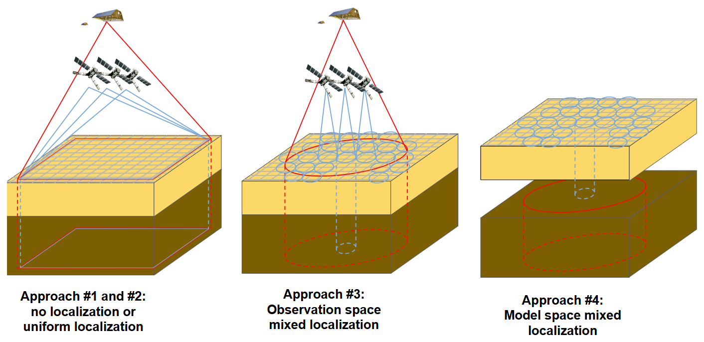
Figure 2 Diagram of different covariance localization approaches considered in this study. In the first two diagrams, the red and blue lines represent the area of influence of TWS and SSM observations, respectively. In the diagram on left (Approach #1 and #2), each SSM and TWS observations can influence a broad area, where spatial update distribution patterns will be constrained by ensemble statistics. In the middle diagram (Approach #3), the influence of SSM observations is concentrated on smaller regions (blue circles), while TWS observations update model estimates in a broader area (red circle) (Eq. 5). In the diagram on right (Approach #4), the blue cylinders represent the model space localization of SSM as well as SSM - groundwater correlations, and the red circle represents the broader model space localization of the groundwater (Eq. 6). The dark brown cube represents the groundwater component of the model, and the yellow cube represents the SSM component of the model.

2.3.6 Model space covariance localization

In addition to observation space covariance localization, it is also possible to implement a model space covariance localization (Campbell et al., 2010) (Fig. 2c). In this approach, localization is applied to the matrix $\mathbf{C}\left({\mathbf{X}}_k^{-}\right)$, which represents the ensemble-based error correlation between the model state variables. In other words, correlations between model grid cells with other model grid cells are damped depending on their distance, no matter the kind of assimilated observation or location of the observations.

The localization is typically performed through smooth distance-dependent functions such as the Gaspari-Cohn function, and applied to the covariance matrix through a Schur multiplication, that is, $\mathit{\rho }\circ \mathbf{C}\left({\mathbf{X}}_k^{-}\right)$ (Campbell et al., 2010), so that the Kalman gain is expressed as

$$\begin{array}{}\text{(6)}& {\mathbf{K}}_k=(\mathit{\rho }\circ \mathbf{C}({\mathbf{X}}_k^{-}\left)\right){\mathbf{H}}^{\top }\left(\mathbf{H}\right(\mathit{\rho }\circ \mathbf{C}\left({\mathbf{X}}_k^{-}\right)){\mathbf{H}}^{\top }+{\mathbf{\Sigma }}_{{\mathit{y}}^o,k}{)}^{-\mathrm{1}}.\end{array}$$

Here, the localization radius should reflect the expected spatial variability of water storage. Although it is possible to define a unique localization radius for all water storage components (see, e.g., Retegui-Schiettekatte et al., 2025b, working with TWS DA), it might be more realistic to consider different localization radii for different vertical water storage components (e.g., a sharper localization might be applied to SSM compared to groundwater, Fig. 2c). This second approach is the one we propose in this study and is from now on called “model space mixed localization”. In a previous work performing daily TWS DA, it was found that the groundwater localization half-radius should be larger than 3° to avoid too sharp groundwater storage updates during DA (Retegui-Schiettekatte et al., 2025a).

Model space covariance localization is especially useful when working with non-local observations (Campbell et al., 2010; Lei et al., 2018), where computing a distance between observations and model variables is not straightforward (e.g., when TWS is assimilated as a sub-basin average, it is not clear which is the “position” of the observation, and taking the geometrical center of the sub-basin as a reference might decrease the influence of the observations around the sub-basin edges). One of its main drawbacks is the need to explicitly calculate the matrix $\mathbf{C}\left({\mathbf{X}}_k^{-}\right)$ (of dimension $\sim \mathrm{34}\mathrm{000}\times \mathrm{34}\mathrm{000}$ in our experiment) and its Schur multiplication with the matrix ρ, of the same dimension, which can be very memory intensive (Campbell et al., 2010).

In this study, four different tuning approaches are compared: Approach #1 is a plain multi-variate DA without tuning; Approach #2 applies observation uncertainty adjustment; Approach #3 applies observation space mixed localization; and Approach #4 applies model space mixed localization (see more details of the implementations in Sect. 3.1). It is worth noting that the Approaches #3 and #4 do not include any observation uncertainty adjustment (Approach #2), and Approach #4 does not require any additional observation space localization such as that in the Approach #3.

2.3.7 Kalman Gain matrix and simplified representation

One of the interesting aspects of this work is the evaluation of the Kalman gain (K) structure in different DA settings (Sect. 4.2). In this section, we delve deeper into the meaning of the Kalman gain and the simplified view displayed in the manuscript.

K (or K_k, where k indicates a specific timestep) is the element in the EnKF equations that determines the extent to which each observation will impact each model variable (see the EnKF equations in Sect. 2.3.1). The structure of K exclusively depends on the model error structure and observation error structure (Eq. 2), and can be modified through DA tuning approaches such as observation uncertainty adjustment and localization (see Eqs. 4, 5 and 6). Note that the final impact of each observation on the model will also depend on the difference between observations and model predictions $({\mathbf{Y}}_k^{\mathrm{o}}-{\mathbf{HX}}_k^{-})$, see Eq. (1), but for the sake of simplicity this factor is omitted from our investigations.

Each column of K corresponds to one observation (i.e., in this study, 3 columns for sub-basin averaged TWS observations, and up to 368 columns for SSM observations). Each row of K corresponds to one model variable (that is, a water storage component in a model grid cell, with 8 water storage components and 4226 model grid cells, resulting in $\mathrm{8}\times \mathrm{4226}=\mathrm{33}\mathrm{808}$ model variables). The matrix element in the row i and column j represents the impact that the observation number j will have on the model variable number i.

Analyzing the structure of K allows us to investigate the impact of each observation on each of the model variables. However, K typically has very large dimensions (33 808×371 in this study), making it difficult to visualize and analyze. To ease this task, in Sect. 4.2 we represent a “simplified view” of K by selecting some representative observations and model variables. In this simplified view, columns 1–3 represent the three sub-basin averaged TWS observations, and columns 4–12 represent 9 selected SSM observations. Likewise, rows 1–3 represent the model sub-basin averaged TWS; rows 4–8 represent model SSM in grid cells for which SSM observations are available and rows 9–12 represent model SSM in grid cells for which no SSM observations are available. The value of each of the matrix elements is represented by a color scale, and the matrix is separated into blocks to facilitate its interpretation. Additional details on the computations of the simplified K displayed in the manuscript are available in Sect. 3.2.

3 Experimental setting

3.1 Model run and DA

3.1.1 Model run

The W3RA model was used to perform the experiments. The model run was carried out for the Ganges-Brahmaputra-Meghna river system area, in a daily and 10 km resolution, with forcing data derived from ERA5 and ERA5-Land (see Sect. 2.2.1). An ensemble size of N_e=30 members was chosen to perform the experiments, following previous TWS and SSM DA experiments (De Lannoy et al., 2022; Springer et al., 2026), together with covariance localization techniques to avoid possible spurious correlations between distant grid cells. The 30 model realizations were generated by perturbing the forcing fields and the parameters of the model according to their own uncertainties, following the approach of Renzullo et al. (2014). The model was warmed up for the period 2000–2003 to reach an appropriate ensemble spread in the water storage estimates. The run was extended from 2003–2015 to generate the Open Loop (OL) solution.

3.1.2 Observation pre-processing

An observation pre-processing was performed before DA. As the modeled and satellite-retrieved SSM typically refer to different soil depths, SSM observations were rescaled so that their statistics match those of the model via cdf-matching (Reichle and Koster, 2005), and the SSM uncertainties provided by ESA CCI were also rescaled accordingly. The ESA CCI tiles for which less than 50 % observations were available were excluded from the DA process (the remaining tiles are colored red in Fig. 1). In the case of TWS, the temporal mean of the sub-basin averaged TWS time series was adjusted to that of the model, but the time series were not rescaled to avoid modifying the amplitude of seasonal, inter-annual and decadal variability, which might be overestimated or underestimated within the model. Both observations were perturbed using a Cholesky decomposition approach and according to their respective uncertainties (Koch, 2007; Schumacher, 2016).

The trends of GRACE TWS in the East and West sub-basins include, among others, ice water loss due to glacier retreat in the Himalayan mountains (Wouters et al., 2019; Li et al., 2023; Sherpa and Werth, 2025), but W3RA does not model glaciers. Glacier retreat rates are available from previous work based on satellite stereo imagery (see Sect. 2.2.1), and therefore a possibility is to exclude these glacier declines from TWS before DA. In the main experiments presented in this study, we do not apply this reduction to equate the experimental conditions to regions where no robust glacier retreat estimates are available. As part of the evaluation, we assess how the W3RA accommodates these trends. Additionally, a side-experiment involving an a-priori glacier trend removal is described and evaluated in Appendix D.

3.1.3 Data Assimilation

All DA experiments were performed for the period September 2003 to December 2015, in the three sub-basins in Fig. 1. The DA update occurs at the end of each daily timestep following the method described in Sects. 2.3.1 and 2.3.2. In addition to the multi-variate DA, uni-variate (i.e., single-observation) TWS DA and SSM DA experiments were also run for comparison.

The TWS observations were assimilated as a summation of all the W3RA land water storage components. SSM was assimilated into the SSM component (that is, in this study, the summation of topsoil and shallow soil components, see Table 2). Although the ESA CCI SSM corresponds to the first few centimeters of the soil, and therefore could be equated to the model topsoil, due to the small field capacity of shallow soil we decided to update these two components jointly. The motivation behind this decision was to simplify the design of the mixed localization for the different localization implementations, as well as the evaluation of the results. Equating a deeper model soil layer with satellite-derived soil moisture could lead to a systematic phase difference between them, where satellite soil moisture variations precede model variations. However, this was not the case in this study, with satellite soil moisture peaking and decaying later in the season compared to model SSM estimates (Sect. 4.3.3). Note that, to further simplify localization and validation, deep soil water and groundwater are also treated jointly (the summation of both is here referred to as groundwater).

In all DA experiments, river water and snow components were excluded from the DA update step as it was found that including them led to degradations in these components (see Appendix D), and the vegetation water storage component was also excluded due to its marginal contribution to the variability of TWS in the basin. The water storage estimates of the river, snow and vegetation of the model were subtracted from the TWS observations prior to assimilation. As a result, only SSM, surface runoff and groundwater components were updated during the DA process.

Spatially, TWS was assimilated as a sub-basin averaged field, and SSM was assimilated as an average over the 0.25°×0.25° ESA CCI tiles (Fig. 1). The observations were downscaled to the model resolution within the DA process through ensemble statistics.

3.1.4 DA tuning approaches

The novel approach suggested and analyzed in this study (Approach #4) implements a model space mixed covariance localization. To the best of our knowledge, this is the first time such an approach has been implemented in a multi-variate land DA experiment. The localization was defined through a Gaspari-Cohn function (see Sect. 2.3.3).

Localization radii in a model-space localization approach should in principle follow the spatial wavelength of water storage variability represented by the model for each component. When analyzing the spatial SSM variability in W3RA, a very smooth variability was found (variations correlated within distances of a few hundreds kilometers), probably due to the coarse parameterization of the model. Since satellite-based SSM observations are likely capable to reflect spatial heterogeneities that are not represented in the model parameters, a localization half-radius 0.5° was applied to SSM (as well as to the covariance between SSM and groundwater) based on the spatial variability that can be expected from SSM observations (see, e.g., Girotto et al., 2019), to allow introducing the observed spatial patterns. Regarding groundwater, the model displayed a decorrelation length of around 300 km, so a localization half-radius of 3° was initially deemed appropriate (based on Retegui-Schiettekatte et al., 2025a). However, this was found to produce very sharp anomalies in groundwater estimates, and finally, a half-radius of 10° was adopted to enhance smoother groundwater variability patterns. In both cases, the values are in the range of TWS localization degrees reported in the literature (see Table 1).

For comparison, three other approaches were implemented based on the previous literature. Approach #1 was a plain multi-variate DA run without any tuning. In Approach #2, (uncertainty adjustment), SSM uncertainty multiplier factors of ${\mathit{\alpha }}_{\mathrm{SM}}=\mathrm{1},\mathrm{2},\mathrm{5},\mathrm{10},\mathrm{15},\mathrm{30},\mathrm{60},\mathrm{240}$ were considered, while α_TWS was kept to 1. Approach #3 (observation space mixed localization) was implemented by applying a smooth localization based on a Gaspari-Cohn function. For consistency with the model space localization, an influence half-radius of 10° was used for the TWS observations and 0.5° for the SSM observations. For the implementation of observation space localization, the TWS observations were assumed to correspond to the center of each sub-basin, and the SSM observations were assumed to be located in the center of each 0.25°×0.25° tile.

3.2 Assessment of the DA performance

For the evaluation and validation stage, all model estimates were averaged over the 30-member ensemble. Standard metrics such as standard deviation (STD), root mean square difference (RMSD), Nash-Sutcliffe efficiency (NSE), Pearson correlation coefficient (here generically referred to as correlation coefficient) and its corresponding p value were used. All validations were performed over the whole study period (2004–2015). A Theil-Sen trend estimate with a Mann-Kendall significance test was used to compute the declines in land water storage in Sect. 4.4.

3.2.1 Kalman gain

The Kalman gain here displayed was computed based on the model covariance structure of the 1st of July of 2004. This date was chosen because of the high correlation between SSM and TWS that appear on this date, which leads to notable cross-variable influences and therefore helps to explain the results observed in the DA experiments. Regarding the observation covariance structure, average errors of 3.31 and 13.38 mm were taken for all SSM and TWS observations, respectively.

3.2.2 Groundwater validation

Groundwater level changes (Δh) were converted to groundwater storage changes (ΔS_GW) using specific yield data (S_y), through the relation $\mathrm{\Delta }{S}_{\mathrm{GW}}=\mathrm{\Delta }h\times S_y$. The groundwater validation is performed on an inter-annual timescale, which is derived by averaging the time series on a sliding window of 12 months. The in situ groundwater time series presented many small gaps that, if left unaddressed, generated larger 12-month gaps after the smoothing process. Therefore, a gap-filling algorithm was applied before smoothing (see more details in Appendix A). For spatial validation of groundwater variability, a clustering based on Principal Component Analysis (PCA) was performed on the observed groundwater level time series (more details on PCA can be found in Forootan and Kusche, 2012; Retegui-Schiettekatte et al., 2025b). Groundwater sites for which the first principal component contributed to more than 65 % of the variability were included in cluster 1, and all other sites were included in cluster 2.

3.2.3 River water level validation

The river water storage validation was performed against in situ water level time series. Comparing river level to river storage requires assumptions on the river cross-section. Due to the absence of this information, we here perform a simple transformation by rescaling the modeled water storage estimates to match the variance of the observed river level data. This is equivalent to assuming a rectangular cross-section and we set the width of the rectangle to obtain a maximum agreement between observed and modeled water levels. Although this approach has many limitations, it does not affect the final conclusion regarding little sensitivity of the model estimates to water storage updates in the seasonal to sub-seasonal timescale (Sect. 4.3.4). The agreement between model estimates and observations was computed in terms of Nash-Sutcliffe efficiency.

3.2.4 Glacier impact computation

For the interpretation of the results in Sect. 4.4, the impact of glacier retreat was reduced from the sub-basin averaged TWS time series. Hugonnet et al. (2021) suggest that glacier retreat does not show strong inter-annual changes between 2004 and 2016 in this region, and therefore we approximated the impact as a linear trend. The trend was calculated as $\mathrm{\Delta }{S}_{\mathrm{subb}}=\mathrm{\Delta }{S}_{\mathrm{glac}}\cdot \frac{A_{\mathrm{glac}}}{A_{\mathrm{subb}}}$, where A_subb and A_glac are the area of each sub-basin and of the glaciers of each sub-basin, respectively, and ΔS_glac is the decrease in water storage produced by the glacier retreat. Glacier trend estimates of previous studies present slight discrepancies, and therefore in this study the largest trend estimate was considered (Table 3).

Brun et al. (2017)Shean et al. (2020)Hugonnet et al. (2021)(Vishwakarma et al., 2022)

Table 3 Glacier trends within the Brahmaputra River basin, as reported in previous literature based on stereo satellite imagery. “w.e.” = water equivalent.

4 Results and Discussion

4.1 Evaluation against assimilated data

In this section, we assess the skill of the new approach proposed in this study, the model space mixed localization (Approach #4), against the assimilated data to verify whether the satellite-derived dynamics were correctly transferred to the target model variables. In addition, we qualitatively evaluate the performance of the assimilation technique in disaggregating its updates into individual storage components based on the model ensemble statistics.

Starting with the original model (Open Loop, OL) estimates, the result suggest a reasonable agreement between the model and satellite observations. GRACE and modeled TWS present a similar seasonality and interannual variability in terms of timing and magnitude (Fig. 3a), and mainly differ in the decadal variability and trend, which is a feature that many hydrological models fail to represent accurately (Scanlon et al., 2018). Model SSM estimates and satellite observations also show similar dynamics from the sub-seasonal to the inter-annual timescale, when averaged over the basin (Fig. 3e).

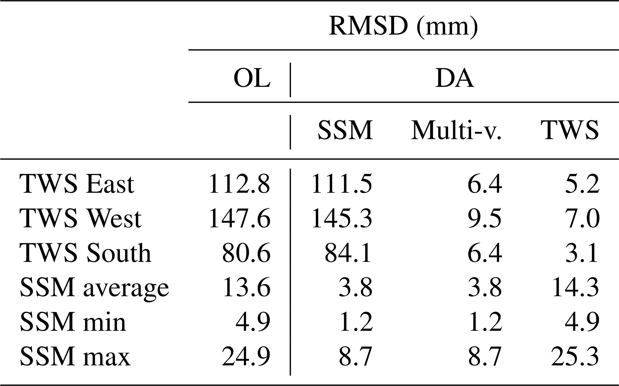
Starting with the uni-variate experiments, evaluating the DA results against the assimilated observations indicates that the observed SSM and TWS dynamics were successfully transferred into the model (Table 4, Fig. 3a–h). The uni-variate SSM DA reduces the RMSD of the modeled and observed SSM from 13.6 to 3.8 mm on average in all 0.25° tiles in which the DA was performed (Fig. 3b). The SSM is found to be predominantly modified during the unsaturated period, changing the timing of the recharge period (April–May) and its decay period (October–March) (Fig. 3a, see also a zoom in a shorter period in Fig. B1 of Appendix B). The uni-variate TWS DA leads to TWS RMSDs below 7 mm for the three sub-basins with respect to GRACE, reflecting a notable improvement with respect to OL TWS which has initial discrepancies of 80–113 mm in terms of RMSD (Fig. 3h). Note that river, snow, and vegetation water storage were excluded from the assessment as these components were not modified in the DA process. The TWS estimates are modified in the seasonal to inter-annual timescale (Fig. 3e), as well as in the sub-seasonal timescale (for example, see June and September 2004 in Fig. B1 of the Appendix B).

Comparing the uni-variate TWS DA results with SSM observations and vice versa can be considered as an independent validation, as only one kind of observation was involved in each uni-variate experiment. The uni-variate TWS DA has a small impact on the SSM estimates (average degradation with respect to OL is less than 10 % of the RMSD value, see Fig. 3d), and the uni-variate SSM DA also shows a very light impact on the TWS estimates (RMSD modified by less than 10 %, see Fig. 3f).

By applying the multi-variate DA, improvements similar to the uni-variate experiments are reached for both SSM and TWS variables, with only minimal differences (RMSD reduced to below 10 mm for sub-basin averaged TWS and an average of 3.8 mm for the 0.25° tile SSM; see Fig. 3c and g). This shows that the setting of the multi-variate DA has correctly constrained the SSM and the summation of all the vertical components.

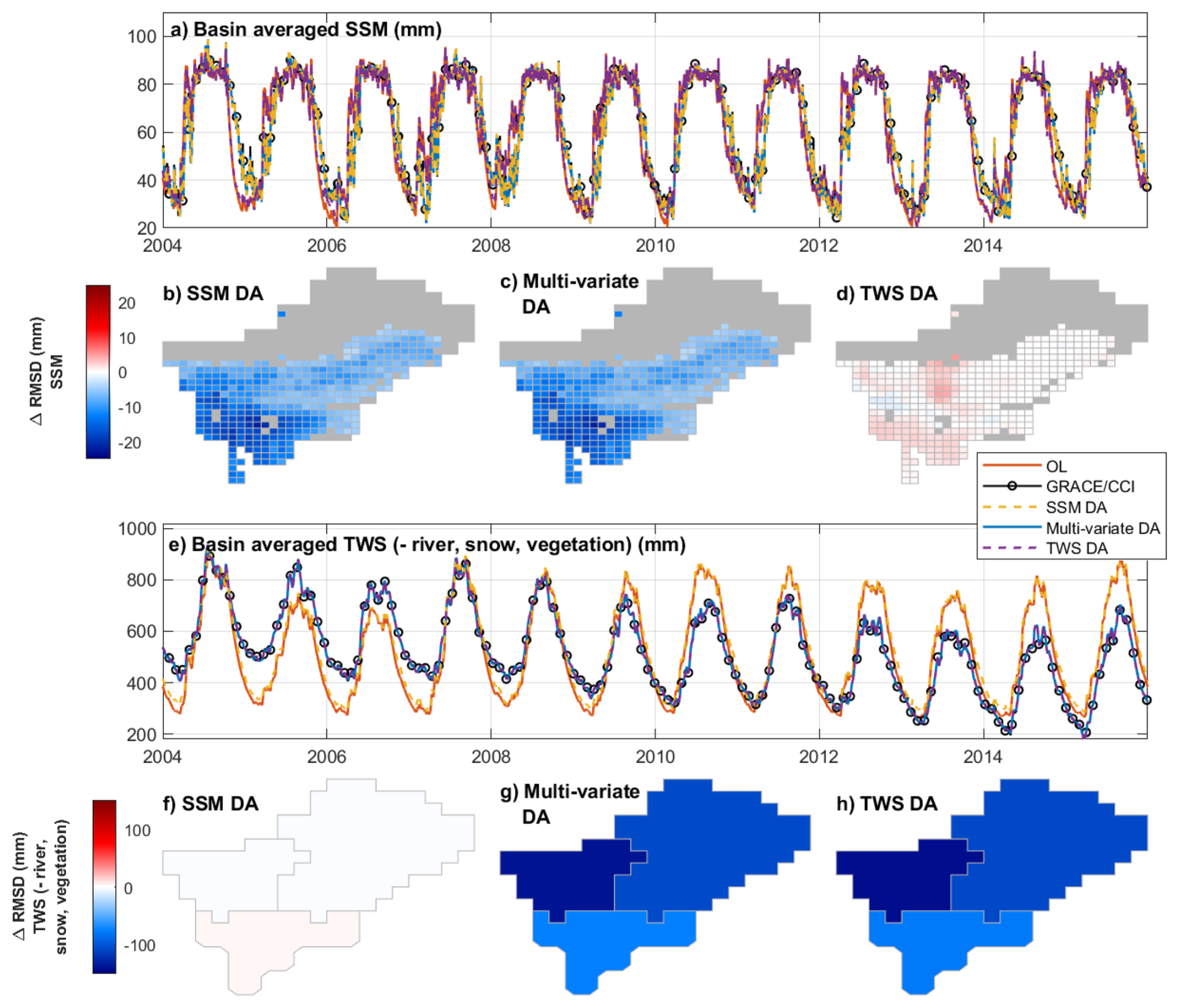
Figure 3 Basin averaged time series of SSM and TWS (a, e) and improvement in the RMSD of tile-averaged SSM (b–d) and sub-basin averaged TWS (f–h) of the model, after different DA experiments. ΔRMSD is defined as the RSMD of the DA product minus the RMSD of the OL, where the RMSD is computed by taking the assimilated data as a reference. (b, f) show the impact of the uni-variate SSM DA, (c, g) show the impact of multi-variate SSM and TWS DA and (d, h) shows the impact of the uni-variate TWS DA. For (b–d), ESA CCI tiles where no observation was assimilated have been shaded (gray area).

Table 4 RMSD of model estimates (OL, SSM DA, multi-variate DA and TWS DA) with respect to assimilated data. SSM min and SSM max refer to the minimum and maximum RMSD values across the 0.25°×0.25° tiles.

A successful modification of horizontally and vertically aggregated variables (e.g. sub-basin averaged TWS or tile-averaged SSM) does not guaranty a realistic update of the underlying distributed estimates (0.1°×0.1° grid) and individual water storage components (Retegui-Schiettekatte et al., 2025a, b). In Fig. 4, the impact of the DA experiments in disaggregated model estimates is represented (in terms of STD with respect to OL estimates).

Regarding SSM, all DA experiments result in a smooth spatial distribution of updates (Fig. 4e-h). It should be noted that regions in which SSM observations were not assimilated (e.g., Himalayan Mountains) are also updated in the multi-variate and TWS DA process (more details in Sect. 4.2).

The negative trends introduced in groundwater show sharp spatial patterns (Fig. 4j-k), leading to notably high RMSD values (up to 3000 mm in some areas of the Himalayan mountains, for multi-variate DA). Different patterns arise in the uni-variate TWS DA and the multi-variate DA; in the latter, areas where SSM is assimilated display smoother groundwater patterns, and sharp patterns are constrained to areas where no SSM was assimilated. This could suggest that constraining soil moisture fields through SSM observations helps regulate the spatial distribution of updates in groundwater. Note that groundwater is the only land water storage component that exhibits negative trends, and therefore this component is likely absorbing the negative trends induced by glacier decline in the East and West sub-basins.

The disaggregation reveals that the uni-variate TWS DA and the multi-variate DA introduce a negative trend to the river water storage estimates (Fig. 4b–d). As the river water component was not included in the DA process, this trend can be fully attributed to decreasing groundwater values, which has a direct impact on streamflow through baseflow generation.

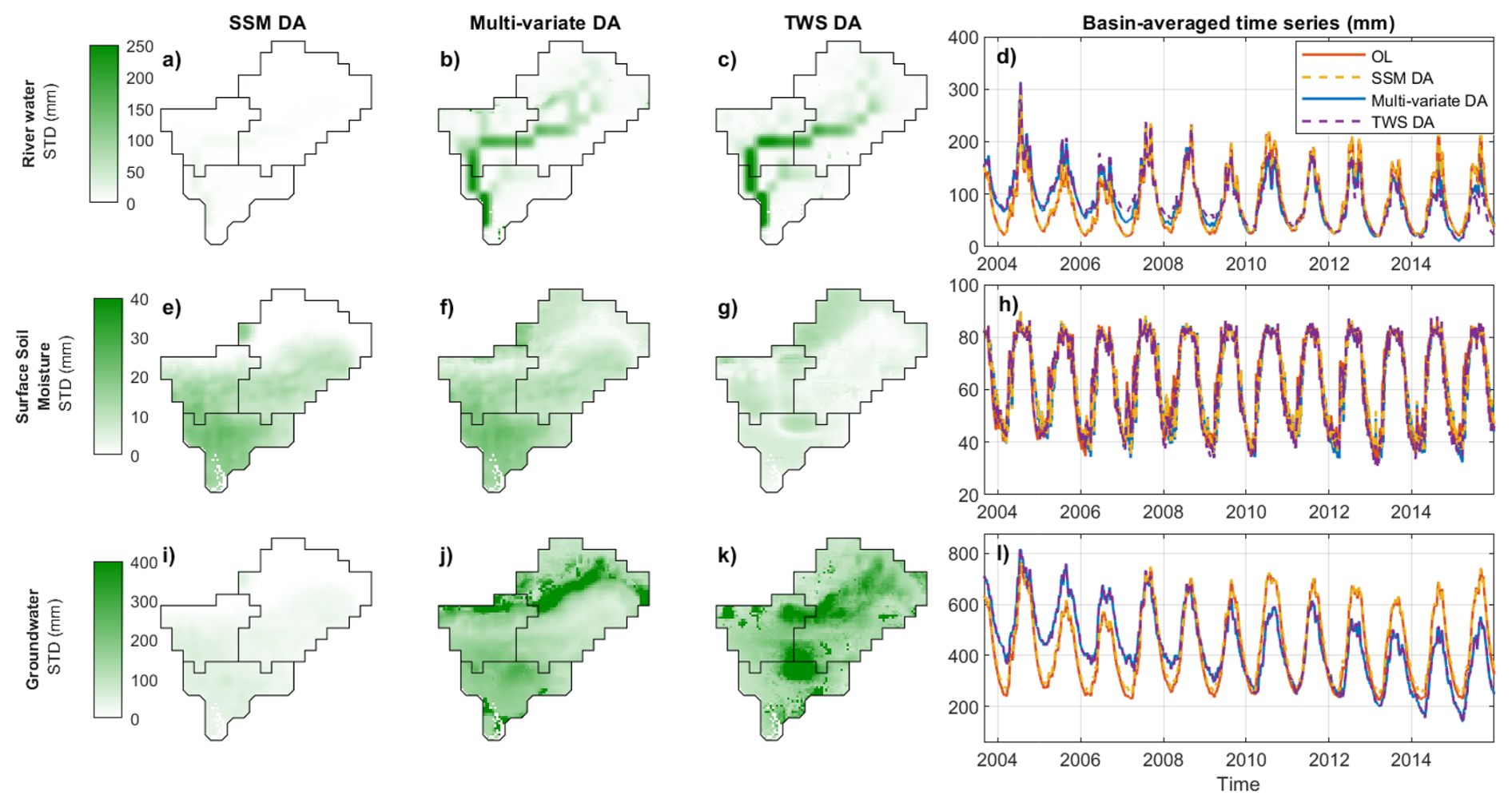
Figure 4 Standard deviation of DA minus OL on spatially distributed (0.1°×0.1° grid) model estimates for river water (a–c), SSM (e–g) and groundwater (i–k). The standard deviation is expressed in mm. The column in the right (d, h, l) shows basin-averaged time series for the same variables.

4.2 Comparing different DA approaches

This section compares the Approach #4 with the results obtained by using other multi-variate DA approaches suggested in the previous literature (Approaches #1–#3). The objective of this comparison is to understand the impact of the different approaches on the DA process and to study the benefits of Approach #4 proposed in this study (see Sect. 2.3.3 for more details of the approaches). In this paper, the descriptions are mostly qualitative, but numerical values can be found in Appendix C.

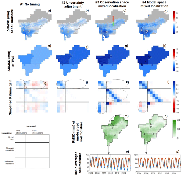
Approach #1 consists of a plain (non-localized and non-adjusted) multi-variate DA. The evaluation shows notable improvements in the SSM component (Fig. 5a), but limited improvements in the TWS estimates (Fig. 5e). More particularly, strong peaks caused by SSM updates in the TWS time series limit the agreement between modeled and observed TWS (Fig. C1 of Appendix C).

This effect is very well reflected in the structure of the Kalman gain matrix (K) for the 1 July 2004. Figure 5i shows a simplified representation of K (see more details on the meaning of K and the simplified representation in Sect. 2.3.7). The impact of the observations on model sub-basin averaged TWS is represented by the intensity of the colors in the upper blocks. We see that SSM observations have an impact that is similar in intensity to TWS observations (upper right and upper left blocks, respectively), reflecting the high influence of SSM observations on modeled TWS.

A similar effect was reported by Tian et al. (2017) where the SSM observations were found to dominate over the TWS observations. They attributed the effect to two factors: (i) the lower uncertainty of the SSM observations (e.g., 3.31 mm on average in our study) compared to the TWS observations (e.g., 13.38 mm on average in our study); and (ii) the higher number of SSM observations (up to 368 per day in this study, due to the 0.25° resolution) compared to the TWS observations (3 sub-basin averaged values per day). Note that Zhao and Yang (2018) reported the opposite effect, with TWS dominating the SSM modifications. In that case, TWS was assimilated at daily, 1°×1° resolution, and the brightness temperature was assimilated at daily, 0.9°×1.25° resolution, that is, both with a similar spatial-temporal sampling. A stationary error of 2 K was used for the brightness temperature and a spatially variable error of unspecified magnitude for TWS. It is therefore possible that, under similar sampling conditions, a too low error for TWS might have favored these observations over the brightness temperature, which would be consistent with the explanation of Tian et al. (2017).

Approach #2: To remedy this issue, Tian et al. (2017) suggested increasing the uncertainty of the SSM observations and reducing that of the TWS observations, to enhance the impact of TWS observations. One of the challenges of this approach is that the appropriate adjustment factor must be found heuristically. In our case, a multiplying factor of α_SSM=10 was found to lead to notable improvements in TWS, but reduce the improvement in SSM (Fig. 5b and f; higher factors lead to degradations in SSM).

The structure of K in this approach shows that the impact of SSM observations on model TWS estimates is considerably reduced compared to Approach #1 (upper right part, Fig. 5j, has lighter colors) but so is their impact on model SSM (central right part). This confirms that the uncertainty adjustment approach offers a compromise between improvements in SSM and TWS, but can be limited due to a significant cross-influence of TWS observations on model SSM and vice versa.

A similar effect was also reported by Tian et al. (2017) explaining that adjusting the uncertainty allows us to reach a compromise between improvements in TWS and SSM, but might not lead to optimal results for these two variables compared to uni-variate DA. The effect was attributed to conflicting constraints introduced by the TWS and SSM observations, which could end up canceling each other. In contrast, Khaki and Awange (2019); Khaki et al. (2019, 2020); Soltani et al. (2024) report an improved performance of some variables in the multi-variate DA experiment with respect to uni-variate DA, suggesting that in those study cases the constraints introduced by TWS and SSM DA in their study region might enhance each other instead of canceling each other.

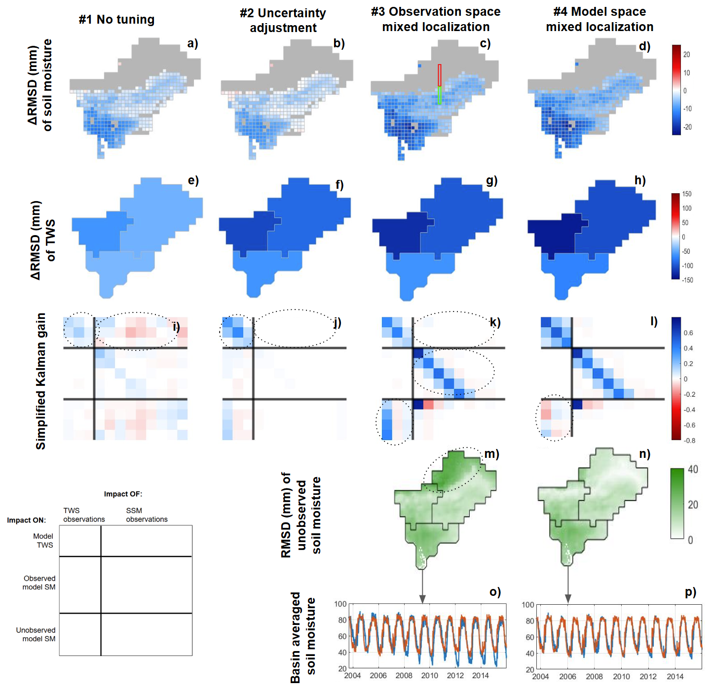
Figure 5 Result evaluation (a–h) and simplified K matrix (i–l) for multi-variate DA with different localization and uncertainty adjustment approaches. The result evaluation includes evaluation of modeled SSM against ESA CCI (a–d), evaluation of sub-basin averaged TWS against GRACE TWS (e–h) and evaluation of unobserved model SSM estimates (m, n), as well as comparison of sub-basin averaged SSM time series of OL (red) and multi-variate DA (blue) (o, p). A guide to interpret the simplified K matrix is provided in the lower left corner (see Sect. 2.3.7 for more details). In (a)–(d), the gray area represents regions where no SSM observation was assimilated due to major gaps in the observations (i.e., Himalayan mountains). The red and green box in (c) show the observed and unobserved model SSM grid cells for which the simplified K is shown.

The approach #3 consists in implementing a mixed observation space covariance localization, similar to that presented by Girotto et al. (2019); Tangdamrongsub et al. (2020) and Wongchuig et al. (2024) (this approach does not include any observation uncertainty adjustment like in Approach #2). The approach is found to lead to notable improvements in both the SSM and the TWS estimates (Fig. 5c and g). Especially, larger improvements are found for SSM when compared to Approach #1 and #2. However, TWS observations are found to have a strong impact on model SSM estimates in areas where no SSM observations are available, such as the Himalayan Mountains (Fig. 5m and the lower left block of K in Fig. 5k). This results in a general negative SSM trend for the entire basin, which is likely unrealistic (Fig. 5o).

Looking at the matrix K provides insight to explain these results (Fig. 5k). First, the localization approach allows to concentrate the impact of each SSM satellite observation in a local region instead of the whole basin (see Fig. 2). This means that each SSM observation can strongly update model estimates in their region of influence, therefore, better modifying the SSM compared to Approaches #1 and #2. Additionally, it means that each SSM observation will have a limited impact at the basin scale (central right block of K in Fig. 5k). As a consequence, the impact of SSM on the sub-basin averaged TWS is kept low without the need of an uncertainty adjustment (upper right block). Second, the impact of TWS observations on SSM estimates is very low for regions where SSM observations are available (left central block), likely because these SSM estimates are already strongly constrained by the SSM observations. The impact is larger for regions where no SSM observations are available (left bottom block). These facts support two conclusions: (i) localization approaches can be used to regulate the relative impact of different observations in a multi-variate DA framework; and (ii) localization can reduce the cross-influence of TWS observations on SSM and vice versa in areas that are constrained by both observations. Note that the key to these two achievements lies in mixed localization, that is, applying different localization degrees for TWS and SSM observations; studies that implement a uniform localization do not report the same results (e.g., Zhao and Yang, 2018)

The results here obtained partly contrast with those reported by Girotto et al. (2019); Tangdamrongsub et al. (2020); Wongchuig et al. (2024), who report a reduced effectiveness of multi-variate DA compared to uni-variate approaches. A likely reason could be the difference on the temporal sampling of the assimilated observations. The daily DA approach used in this study might be more successful at constraining the model, when compared to sequential or asynchronous assimilation approaches that do not assimilate both observations simultaneously. The fact that either TWS or SSM is unconstrained during the DA update could have enhanced the cross-influence between them, leading to problems when the observations introduce conflicting or anti-correlated updates. Although this explanation is plausible, further investigation is needed to confirm it and better understand how the cross-variable influence works in asynchronous DA.

Finally, Approach #4 (model space mixed localization) displays similar benefits as Approach #3 (Fig. 5d and h) and additionally reduces the impact of TWS observations on SSM in areas where no SSM observations are available (Fig. 5n), effectively preventing spurious trends in the SSM component (Fig. 5p). The key here is that localization is performed on the model space instead of the observation space (see Fig. 2), allowing to localize the impact of observations on the model SSM estimates over the whole basin, regardless of the availability of SSM observations.

In the K matrix (Fig. 5l), this can be seen in the left bottom block, showing a less intense impact of TWS observations on unobserved SSM estimates compared to Approach #3. It should be mentioned that these results are sensitive to the chosen groundwater localization radius; more details on the extent of this sensitivity is provided in Appendix D.

In summary, among the four strategies tested, Approach #4 is found to be the only one capable of reducing the influence of TWS on SSM, thus marking a first in addressing the cross-variable interference reported in previous studies. It is worth mentioning that model space localization is particularly suited for the integration of sub-basin averaged (i.e., non-local) observations, where defining an observation space localization can be challenging (Campbell et al., 2010). This approach was also found to avoid cross-variable influences in uni-variate TWS DA (see Sect. 4.1).

One of the main limitation of this approach lies in the computational demand, as it requires the computation of the full model covariance matrix and a Schur operation in the model domain (Houtekamer and Mitchell, 1998; Campbell et al., 2010). This highlights the need for optimized implementations.

Another approach that could possibly help avoid cross-variable influences is the application of a vertical observation space localization, aiming at concentrating the TWS update in the groundwater and the SSM update in the soil moisture. This approach was not considered in this study because the implementation of such localization is not straightforward, especially in the land hydrology system where water propagates vertically, and therefore water storage dynamics can be highly correlated across vertical storage components. Future studies could focus on proposing an adequate implementation of this approach and evaluating its potential benefits and limitations.

4.3 Evaluation against independent data

In this section, we compare the DA results with independent data to test if the assimilation of TWS and SSM succeeds in bringing the model closer to reality. In light of the assessment of Sect. 4.2, we expect Approach #4 (model space mixed localization) to lead to the best results and therefore here we only present the validation of the multi-variate DA using Approach #4.

4.3.1 Terrestrial Water Storage

We evaluate the realism of the assimilated TWS dynamics using the independent SPEI-12 drought index. Because SPEI is derived from climatic water balance rather than direct observations of storage, the comparison is interpreted as a consistency check rather than a strict validation.

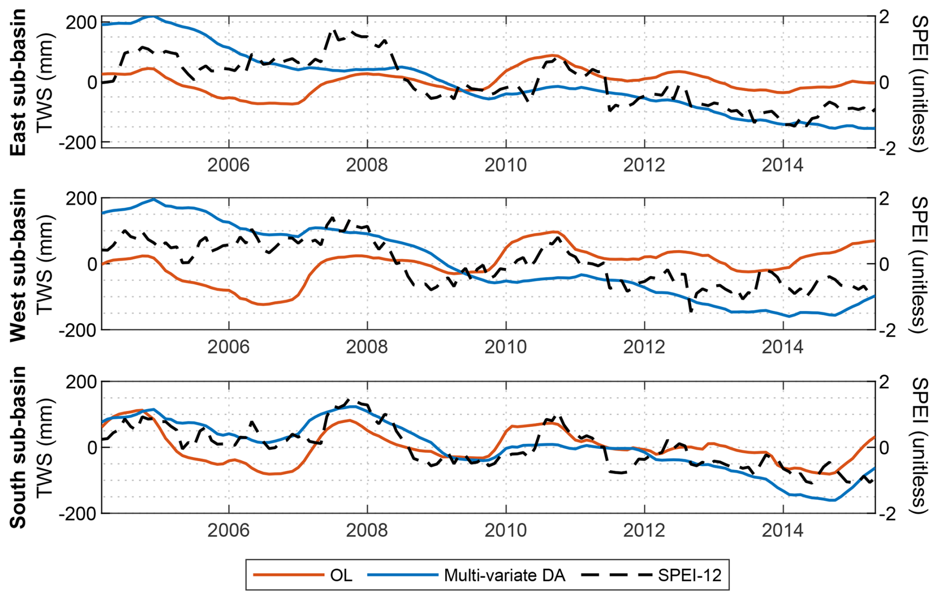
Figure 6 Inter-annual TWS variability of OL and multi-variate DA for the three sub-basins; SPEI time series are plotted in the right axis.

Although SPEI is standardized and is not suitable for validating the magnitude of TWS variability, it reveals clear negative trends for the three sub-basins in the period 2004–2014 (Fig. 6). These trends are absent in the OL simulations. The disagreement could partly originate from model limitations, such as a limited representation of evaporation in surface water bodies, or vegetation and transpiration. However, it likely also reflects a more general difficulty of hydrological models to represent decadal TWS variability and trend related to climate variations and human water use, as reported in a multi-model experiment by Scanlon et al. (2018).

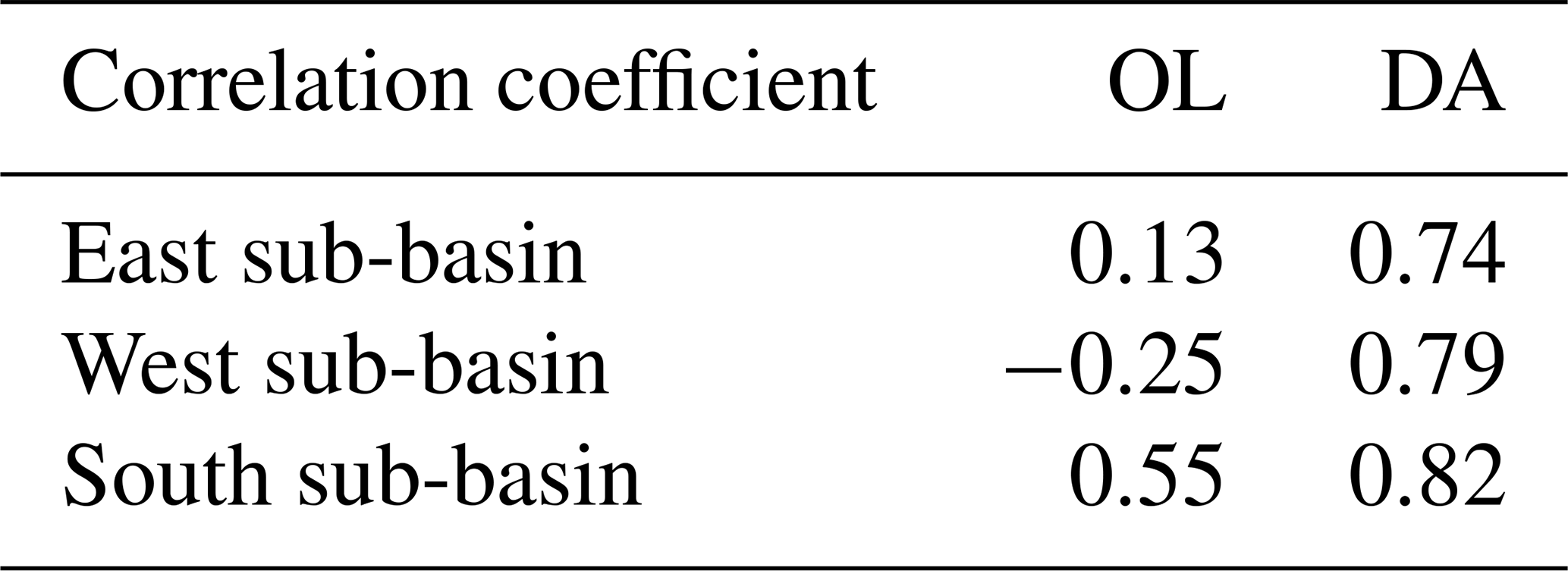
The decadal trends emerge distinctly through the multi-variate DA. Regarding the sub-decadal variability, multi-variate DA preserves the inter-annual variability of OL, although it also excessively smooths certain anomalies (e.g., 2007 and 2010), possibly due to GRACE TWS resolution or interference with the decadal trends. In general, the correlation with SPEI is significantly improved through DA from 0.13/−0.25/0.55 (OL) to 0.74/0.79/0.82 (DA) for the East, West, and South sub-basins, respectively (Table 5). An especially large improvement is observed in the West sub-basin, where the OL estimates suggest a positive TWS trend as opposed to the DA TWS and SPEI data.

Table 5 Correlation coefficient between modeled TWS and SPEI. All correlations are significant with p value < 0.01.

4.3.2 Groundwater

We compare groundwater estimates in the South sub-basin against monthly groundwater storage changes derived from in situ observations, to assess the realism of their temporal and spatial patterns.

To convert groundwater level observations to groundwater storage data, spatially distributed specific yield data from Shamsudduha et al. (2011) was first used (see Sect. 2.2.1 for more information). The results show a significant scale difference between the modeled and observed groundwater variability, both in the seasonal timescale (STD of 182 and 140 mm for OL and DA respectively, and 65 mm for observations, Fig. 7a) and the inter-annual timescale (STD of 35/50/14 mm for OL, DA and observations respectively, Fig. 7c).

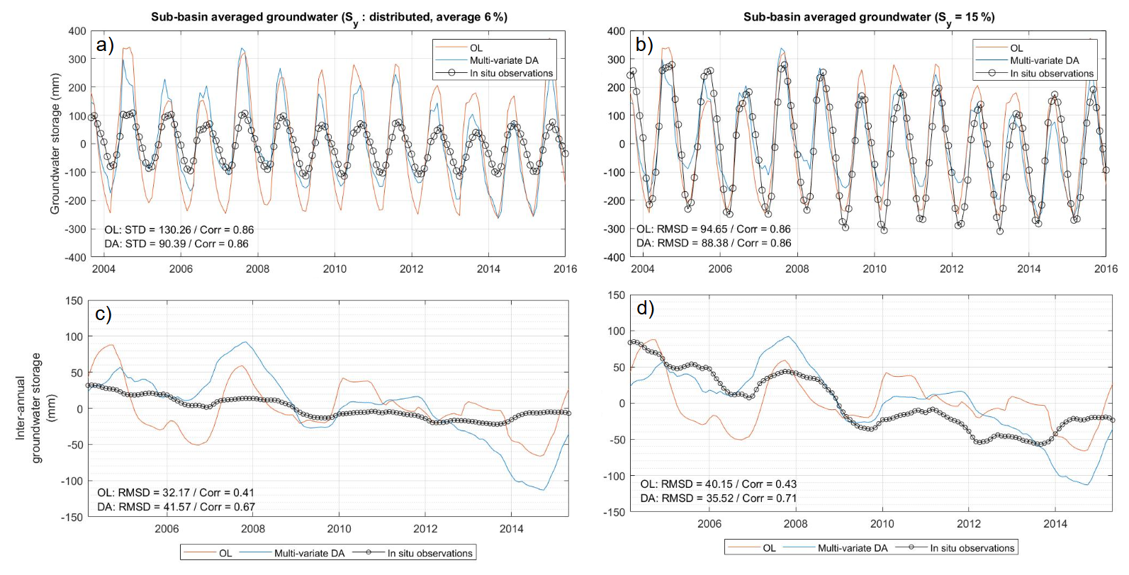
Figure 7 Inter-annual groundwater storage variability derived from OL, multi-variate DA and in situ groundwater level observations. a and b represent the time series, and (c) and (b) represent their inter-annual variability component. In (a) and (c), the observed groundwater storage was computed using distributed yield values computed by Shamsudduha et al. (2011). In (b) and (d), a uniform specific yield value of 15 % was used.

Various reasons could be behind this discrepancy in magnitude, which concern both the groundwater level observations and the model. On the observation side, the groundwater wells used for validation in this study measure water levels in shallow aquifers with a mean depth of 30 m (Shamsudduha et al., 2012), while the model and GRACE water storage changes reflect water mass variations at all ground levels including deep aquifers, and can therefore be expected to present a larger variability (see, e.g., Qu et al., 2024). The specific yield values used to convert observed groundwater levels to groundwater storage values can also be affected by biases and uncertainties (Rodell et al., 2007): factors in its measurement, such as an insufficient duration of the pumping test or the assumption of partial penetration, can lead to an underestimation of the specific yield, consequently leading to an underestimation of groundwater storage variability. The spatial interpolation of specific yield data, which was performed based on ground lithology maps (Shamsudduha et al., 2011), can additionally contribute to their uncertainty.

On the model side, an inadequate partitioning of the soil profile in its different layers could result in attributing part of the soil water storage variability to the groundwater component (Sun et al., 2010; Shamsudduha et al., 2012). In theory, general model limitations to represent water storage variability could also contribute to this discrepancy, although this possibility is here considered less likely due to the good agreement found between W3RA and GRACE TWS variability (Sect. 4.1).

To avoid the impact of possible uncertainties in the specific yield data, a second comparison was performed by considering a uniform specific yield of 15 % for all the groundwater wells, which is close to values of 10 % used by Shamsudduha et al. (2012) for Bangladesh or average values of 14 % reported by Rodell et al. (2007) for the US in previous studies. This significantly increases the magnitude of the observed groundwater variability (STD of 171 mm in the seasonal timescale and 40 mm in the inter-annual timescale, Fig. 7b and d). The new comparison suggests that the agreement between modeled and observed groundwater is increased, and RMSD is reduced from 95 to 88 mm after DA. Especially, the DA results display a high agreement with observed data during the wet periods, as also reported by Shamsudduha et al. (2012), although the DA results seem to slightly underestimate the seasonal amplitude when compared to the OL. In the inter-annual timescale, DA reduces the RMSD from 40 to 36 mm (Fig. 7d).

To ensure that the results obtained are not an artifact of the chosen specific yield, the comparison is repeated in terms of Peason correlation coefficient, a metric that is scale invariant. Improvements are especially observed in the inter-annual timescale (Fig. 7d), in which the correlation with observed groundwater storage is increased from 0.43 to 0.71 after DA. Especially, the groundwater storage derived from DA presents a negative trend for the period 2004–2014, with higher levels in 2005–2008 than in 2013–2014, which is clearly featured in the observed data and not reflected in the OL model estimates. DA also displays realistic sub-decadal variability, capturing key anomalies such as the 2007 peak and the wet period of 2010–2011, which remain distinguishable despite the overarching negative trend.

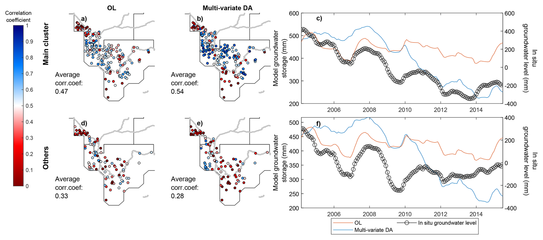
Figure 8 (a, b, d, e) Correlation coefficient between modeled groundwater storage and observed groundwater level for individual sites. The centerline of the main rivers of the region are added in the background as a reference. (c, f) Average groundwater storage and groundwater level time series for sites belonging to the main cluster (c) and remaining sites (f).

To evaluate the realism of spatial groundwater patterns of the DA results, a comparison against distributed groundwater time series provided by individual wells is shown in Fig. 8. Biases in the specific yield estimates are likely to be more severe when the assessment is performed for specific wells, and therefore this comparison is exclusively performed in terms of correlation coefficient.

The results show that DA improved groundwater estimates in many parts of the basins, but also suggest degradations for some specific sites and regions (Fig. 8). To better interpret the results, a PCA-based clustering of in situ data is applied (see details in Sect. 3.2). For the sites belonging to the main cluster (Fig. 8a, b, and c), overall improvements are observed as a consequence of the negative trends introduced by the multi-variate DA process, increasing the average correlation coefficient from 0.47 (OL) to 0.54 (multi-variate DA). Certain short-term anomalies, such as the positive anomaly in 2010–2012, may appear better represented in the OL solution, posing a need for further investigation in future studies, particularly to assess potential links to sub-decadal glacier- or snow-related anomalies (Li et al., 2025). Conversely, other anomalies, such as the 2007–2009 event, are more accurately reproduced by the multi-variate DA.

For the remaining sites (Figs. 8d and e), of which most are located close to the main rivers branches, notable degradations can be observed. Multi-variate DA introduces a negative trend in these regions too, but the observed groundwater level of this cluster is characterized by a less strong trend, which reduces the average correlation from 0.33 (OL) to 0.28 (multi-variate DA). The absence of trend in the observations might be explained by the fact that large river branches in these regions allows greater groundwater recharge, either through natural percolation processes or enhanced by anthropogenic actions (Shamsudduha et al., 2022). W3RA does not account for the feedback from the surface to the sub-surface components and therefore the DA is not informed about this mechanism.

In conclusion, the multi-variate DA appears to improve the overall groundwater storage dynamics in the South sub-basin, especially through the modification of inter-annual groundwater variability and the introduction of a negative trend for the period 2004–2014 that is also reflected in groundwater level observations. It is important to note that the comparisons performed here validate the groundwater dynamics but not magnitude of the trend, due to uncertainties in the scale between the modeled and observed groundwater data. Namely, the magnitude of the DA trend and inter-annual variability could be overestimated due to the over-allocation of surface water or shallow soil variability to the groundwater component in the DA process.

4.3.3 Surface soil moisture

Here we compare the OL and DA outputs with the soil simulations of the WaterGAP global hydrology and water use model (Döll et al., 2003; Müller Schmied et al., 2024; Nyenah et al., 2025). Although model outputs might be affected by limitations such as errors in forcing data, process simplification, or missing representation of certain processes, they can provide an additional perspective to perform a consistency check and assess the realism of the DA results.

The basin averaged time series show that, after multi-variate DA, SSM becomes saturated later in the season, and the decay of water at the end of the monsoon season is also slower (Fig. 9a). In other words, DA results mainly in a light phase shift in the SSM time series. The phase shift brings the estimates closer to those of the WaterGAP estimates.

Regarding the spatially distributed estimates, original W3RA (OL) estimates present an especially strong discrepancy with WaterGAP in areas with a sharp topography (slope > 1 %, correlation coefficients mostly between 0.4–0.7, see triangles in Fig. 9b). After DA, notable increases in the correlation with WaterGAP arise in these mountain regions, reaching increases of up to +0.3 correlation points in areas where SSM observations are available (Fig. 9c).

There could be various reasons why the two models disagree in mountainous areas. WaterGAP is calibrated for the Brahmaputra River basin and is able to reflect a broader range of land cover conditions and soil compositions (Müller Schmied et al., 2021) when compared to the W3RA model (van Dijk et al., 2013). This could make the WaterGAP model more suited to represent land surface hydrological processes in areas with a sharp topography such as the Himalayan Mountains. Taking this into account, the results could indicate that the assimilation of ESA CCI SSM helps to better account for SSM variations in topographically complex areas. However, these results should be interpreted with caution, as the WaterGAP model might also be affected by its own limitations in other aspects.

The observed differences could also be related to the depth considered for the SSM components, which is larger in WaterGAP when compared to W3RA. To exclude this possible cause, we have repeated a comparison equating WaterGAP SSM with the summation of all soil water storage components of W3RA (that is, topsoil, shallow soil, and deep soil, see Table 2). The results, reported in Appendix F, lead to conclusions similar to those presented here, thus excluding the depth difference as the origin of the disagreement.

An important consequence of these results is that the assimilation of SSM could be accounting for the limited performance of the W3RA model at estimating SSM variability in mountain areas, but it is not clear if improvements could be expected from the assimilation of SSM products if a better adapted base model was used (e.g., WaterGAP itself). Evaluating the added value of the satellite-based SSM product with respect to different hydrological models is not within the scope of this study, but should be considered in future satellite SSM DA experiments, especially regarding its operational implementation.

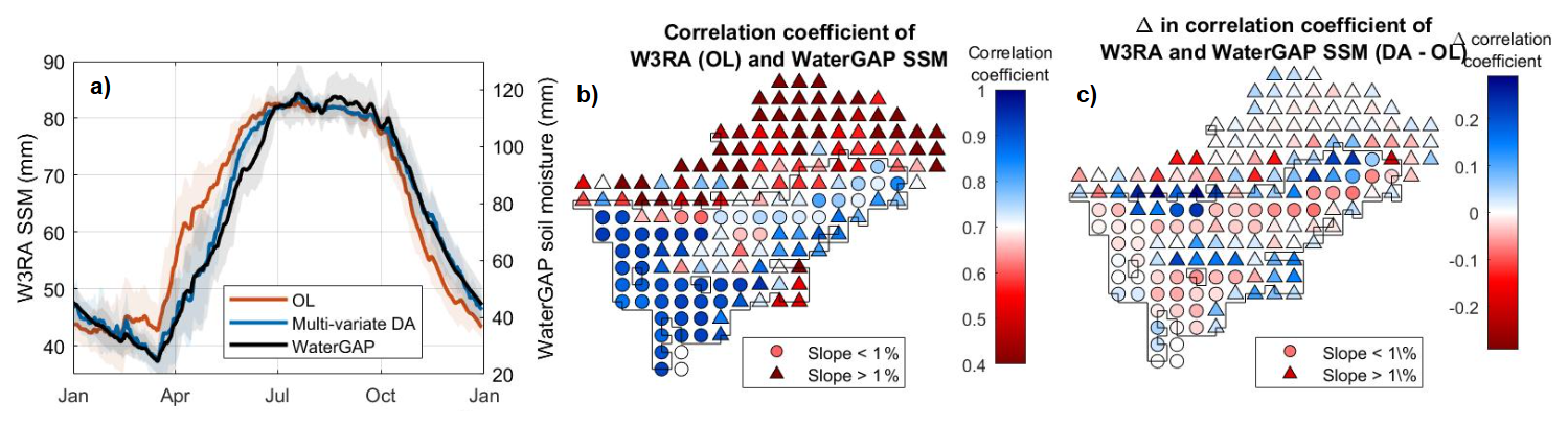
Figure 9 (a) SSM seasonality of W3RA OL, multi-variate DA and WaterGAP. (b) Distributed map of correlation coefficient of W3RA (OL) and WaterGAP, shown for the WaterGAP 0.5°×0.5° tiles. (c) Distributed map of change in correlation coefficient between W3RA and WaterGAP after DA. The black outline in (b) and (c) indicates the area where SSM observations were assimilated.

In the more flat regions located along the Brahmaputra River (slope < 1 %, circles in Figs. 9b and c), for which the W3RA OL and WaterGAP estimates are more similar (correlation coefficients between 0.7–1.0), DA is found to slightly reduce the agreement between the two models by up to 0.1 correlation points. For the Himalayan Mountain area, where no SSM observation was assimilated, the impact of DA is driven by the TWS observations and leads to slight improvements and degradations.

4.3.4 River water

River water storage estimates are here validated against in situ river water level observations. We select the two sites that are closest to the outlet of the West and South sub-basins (water level data is not available for the East sub-basin, see site locations in Fig. 1). Comparing river level to river storage requires assumptions on the river cross-section. Due to the absence of this information, the modeled water storage estimates were rescaled to match the variance of the observed river level data before validation (Sect. 2.2.1). Although this approach has important limitations, it does not affect the main conclusions described in what follows.

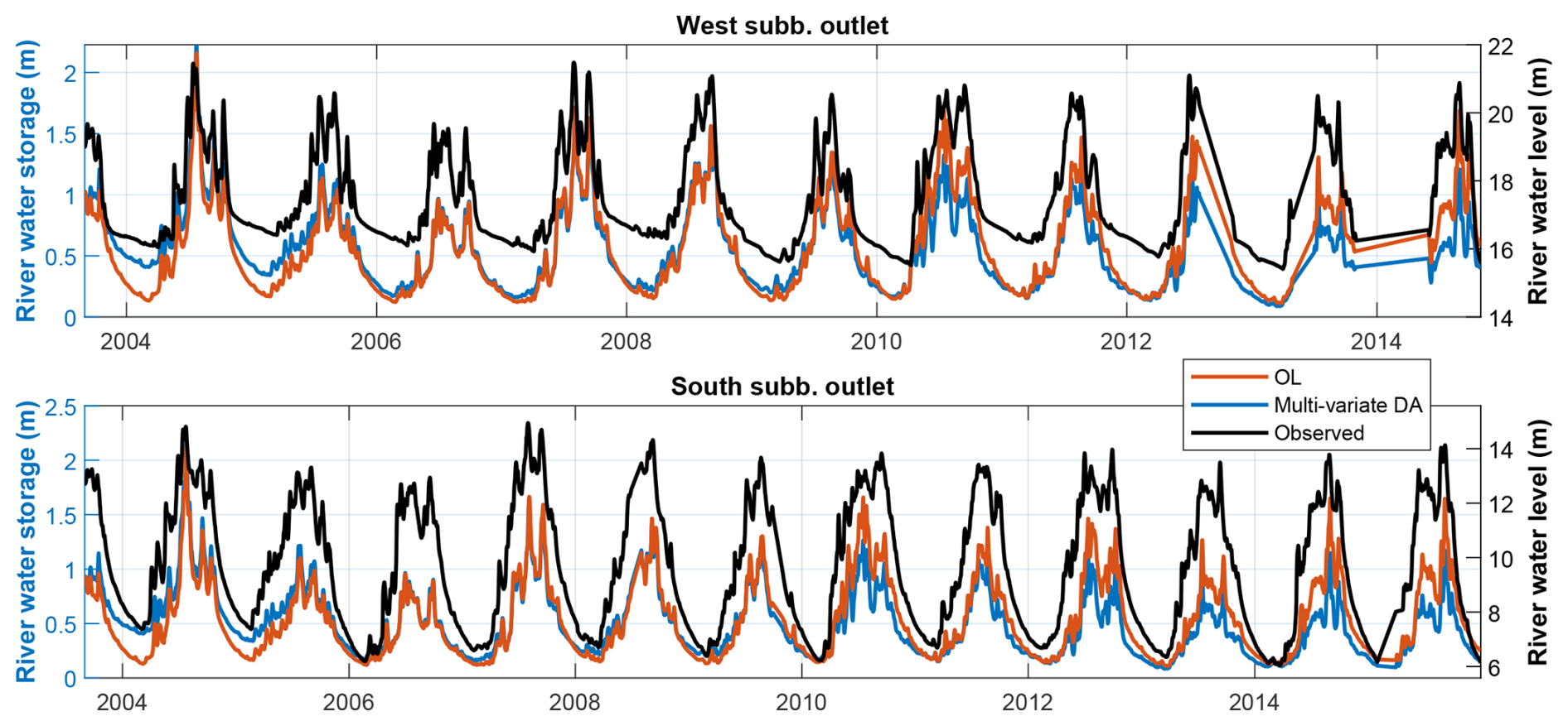
Figure 10 River water storage time series derived from OL (red) and multi-variate DA (blue), as well as in situ water level observations (black, with y axis on the right). The time series correspond to the two sites shown in Fig. 1.

The OL time series show dynamics similar to the observed water levels (Fig. 10), with a high Nash-Sutcliffe efficiency (NSE) of 0.84 and 0.83 for the West and South sub-basins, respectively. The multi-variate DA introduces a decadal negative trend and inter-annual variability in both sub-basins, as can be noted by the higher river water storage values in 2004–2005 and notably lower values after 2010. As a consequence, the NSE is reduced to 0.75 and 0.74 for the West and South sub-basin, respectively, after DA.

Although river water storage was not directly updated during our DA experiments, the observed changes in river water storage likely stem from trends and inter-annual variability introduced in groundwater by multi-variate DA, which then have an impact in streamflow through baseflow generation. Re-visiting runoff parameterization or applying joint Calibration/Data Assimilation (CDA; Eicker et al., 2014; Schumacher et al., 2018) could help refine this process. In addition, groundwater also includes negative trends related to glacier retreat (see Sect. 4.1), which likely increases negative trends in river storage. Incorporating a glacier component into the model representation and guaranteeing an accurate TWS trend partitioning between glacier and groundwater could help mitigate this issue.

Validation using detrended time series yields NSE values of 0.84/0.84 (OL) and 0.86/0.82 (DA) for the West and South sub-basins, respectively, suggesting that multi-variate DA has limited influence on sub-annual river storage dynamics. This aligns with the findings of Ahmad et al. (2024), where SMAP SSM assimilation into Noah-MP showed minimal impact on streamflow in high-flow tributaries such as the Brahmaputra River. The broader literature also points to methodological choices, catchment characteristics, and land–river coupling limitations as key factors that restrict the impact of DA on river discharge (Massari et al., 2015; Brocca et al., 2017). As a consequence, this comparison cannot be further utilized to validate the hydrological estimates obtained through the DA experiment.

It is worth mentioning that we also attempted a multi-variate DA experiment in which we updated the river water storage component together with the land water storage states. The results are reported in detail in Appendix D, which show significant degradations in the sub-seasonal timescale. This suggests that to improve the surface water component in the Brahmaputra River basin, a direct DA of water level measurements, such as lake and river altimetry, might be more beneficial than a SSM and TWS DA (see, e.g., Wongchuig et al., 2024).

4.4 Land water storage variability in Brahmaputra River Basin

The DA outputs show a higher realism than the initial model estimates (as shown in Sect. 4.3) while keeping the spatial and temporal resolution and continuity of the model. This leads to improved land water storage estimates that can be used to better monitor and understand the land hydrological variability of the Brahmaputra River basin. Here we perform a characterization of land water variability for the basin.

The basin averaged land (+ river) water storage time series is shown in Fig. 11. Since the glacier mass loss has been quantified in previous studies based on satellite stereo imagery, the glacier trends have here been reduced from the TWS estimates to explore the variability related to land water (see more details in Sect. 3.2).

The time series show a strong seasonal variability marked by the monsoonal climate regime. The middle line shows the inter-annual variability, which displays similar temporal patterns to those found for groundwater in Sect. 4.3.2. A Theil-Sen trend estimate reveals a significant decrease in land water storage of −15.2 mm per year for the period 2004–2015 (p value < 0.01 in the Mann-Kendall test), which translates to a loss of 70.9 GT (gigatones) of water per decade. This suggests that, according to current estimates of glacier trends, the Brahmaputra River basin lost approximately as much land water as glacier water during the study period (with 67.5 GT lost due to glacier retreat). These numbers should be interpreted with an uncertainty at least as high as that of glacier retreat, estimated at up to ±0.17 m water equivalent per year by Shean et al. (2020) (Table 3), equivalent to ±18.9 GT per decade. The drivers of these land water storage trends could be both natural climate variability and anthropogenic activities, and will be further explored in a future study. No significant storage trend is detected in the SSM component, although dryness and wetness conditions could affect the SSM in the duration of the saturation period (to be assessed in a future study).

The TWS also displays a considerable inter-annual variability (std of 22 mm on detrended time series). For example, during the years 2007 and 2010, the basin gained 15.9 and 13.5 GT of water, respectively. In fact, these two periods have been reported as wet years in which extended flooding events occurred in the basin (Rao et al., 2020; Brakenridge, 2024). The impact of the wetness-dryness periods is found to have a stronger expression in the annual maximum values (SD of 70 mm in detrended time series, upper pointy line in Fig. 11) than the minimum values (std of 26 mm in detrended time series, lower pointy line in Fig. 11), likely due to the contribution of the river water mass during high river flow events.

The DA process provides uncertainty values for model estimates, which are computed based on ensemble statistics. The statistics suggest an average standard deviation value of 15 mm for TWS, with a maximum value of 36 mm in periods with a high water storage variability, which is rather low compared to the large seasonal variability of TWS. However, these values are likely underestimated, since the uncertainty of daily GRACE TWS used in this study was approximate due to the absence of exact estimates, and possible temporal autocorrelation in observations were not accounted for (Sect. 2.2.1). Future studies quantifying the magnitude and structure of sub-monthly TWS errors will enable more robust DA frameworks that are able to represent model variable uncertainties with increased realism.

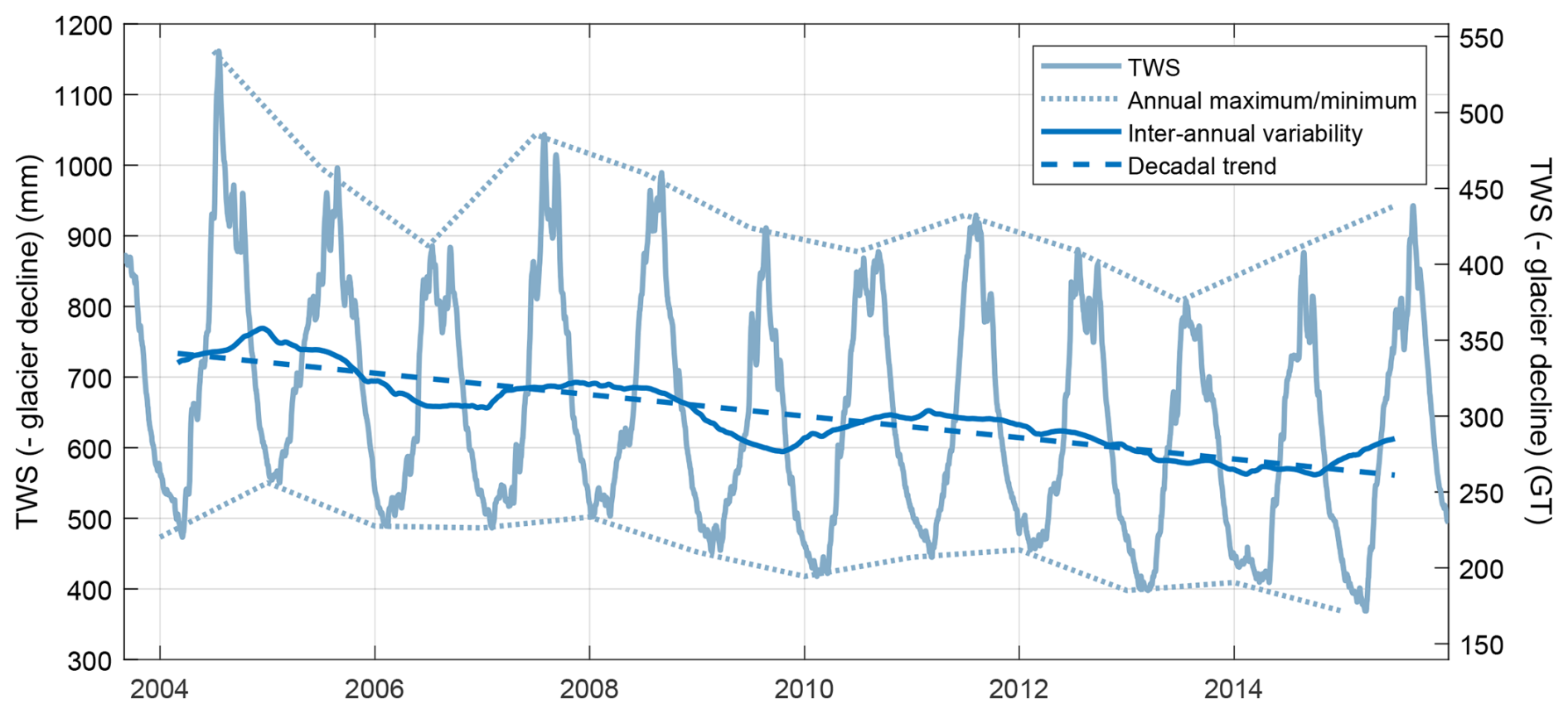
Figure 11 Basin averaged TWS (− glacier decline) for the Brahmaputra River basin from Approach #4. The left axis shows the TWS in mm, while the right axis shows the TWS in GT (gigatones).

5 Conclusions

This study presents a daily-scale multi-variate Data Assimilation (DA) experiment for the Brahmaputra River basin, integrating TWS and SSM observations. In contrast to previous studies that assimilate GRACE TWS in a monthly timescale, the daily DA in this study enabled the assimilation of hydrological dynamics across multiple temporal scales, ranging from sub-monthly variability to decadal trends. The daily implementation also avoided model-observation temporal mismatch that typically requires complex smoothers or multi-step DA frameworks (Tian et al., 2017; Girotto et al., 2019; Tangdamrongsub et al., 2020), and thus allowed us to explore other aspects of the DA mechanism. The study pursued two main objectives: (i) investigating how different multi-variate DA approaches influence the DA mechanism and address limitations reported in the prior literature, and (ii) generating improved land water storage estimates for the basin, allowing a refined analysis of its hydrological variability.

For the first objective, we considered three existing and one new multi-variate DA approaches and analyzed their impact on the Kalman gain matrix and assimilation outcomes. Conventional uncertainty adjustment approaches (Tian et al., 2017) and observation space localization approaches (Girotto et al., 2019; Tangdamrongsub et al., 2020; Wongchuig et al., 2024) are useful to balance the influence of the different observations, but are affected by significant cross-variable interference, that is, TWS can strongly impact model SSM estimates, especially in regions where SSM is unconstrained. This is not necessarily a harmful effect and can be desirable in some circumstances to help address errors in observational datasets or in cases where TWS and SSM DA updates might enhance each other (see, e.g., Khaki and Awange, 2019; Khaki et al., 2019, 2020; Soltani et al., 2024). However, previous studies in multi-variate land DA report that this cross-variable interference can lead to a diminished performance in multi-variate DA due to conflicting constraints or anti-correlated updates induced by the two observation sets (Tian et al., 2017; Girotto et al., 2019). As an example, in our study spurious decadal negative trends were introduced in the unconstrained SSM estimates when observation space localization was implemented.

To overcome this issue, we introduce a model space mixed covariance localization approach, which applies localization directly to the model covariance matrix. This method successfully regulates cross-variable influence for the first time, both in the uni-variate as well as the multi-variate DA, offering a way to address one of the most important challenges reported in multi-variate land DA literature so far. An additional interesting property of model space localization is its adequacy for assimilating spatially averaged (i.e., non-local) observations such as TWS (Campbell et al., 2010). It should be noted that, although the W3RA model was taken as a baseline for these experiments, the methods explored in this paper could be applied to any hydrological model. The main drawback of this approach is that it requires explicit computation of the model covariance matrix and a Schur multiplication with the localization matrix, posing significant computational memory demands and motivating future work on its optimization. The results were also found to be sensitive to the localization radius, which should be chosen with caution.

For the second objective, validation against SPEI and in situ groundwater data shows that multi-variate DA substantially improves TWS and groundwater estimates, capturing both decadal trends and inter-annual variability and thus bringing the model closer to reality. A limitation of this study is the absence of independent SSM observations to validate the model dynamics. To overcome this, a consistency-check was performed by comparing the estimates to those obtained by the WaterGAP model, which is in principle better adapted to represent high-mountain environments. Based on this comparison, SSM estimates show notable improvements near mountainous regions, aligning more with WaterGAP estimates.

The enhanced DA time series enabled a robust characterization of hydrological variability in the Brahmaputra River basin, revealing a net water loss of 70.9 GT in 2005–2015 and pronounced inter-annual fluctuations. These refined estimates pave the way for further research into the drivers of land water variability and its expression in different hydrological components. Future work will explore the role of land water storage in flood generation and extend the analysis to the entire GRACE/GRACE-FO period (2002–2025), allowing for identification of bidecadal trends and an improved understanding of the dynamics of extreme events in the region.

Appendix A: Gap-filling algorithm

The monthly in situ groundwater level observations presented some minor gaps that needed to be filled. The following algorithm was found to perform satisfactorily for the study region. (This algorithm was applied to each in situ site independently).

1. Perform a Least-Squares regression to compute the mean and seasonality of the signal.

2. Fill the gaps with the values predicted by the Least-Squares fit.

3. Compute inter-annual variability of the signal, save it in auxiliary variable and deduce it from the signal.

4. Repeat step 1 and 2 over the signal with reduced inter-annual variability.

5. Add the inter-annual variability back to the signal.

This algorithm allows to fill the gaps in time series for which the seasonality can be approximately parameterized through a simple model, but the inter-annual variability is more difficult to parameterize due to its non-stationary nature. A PCA-based algorithm was also attempted, but did not work so well, likely due to the very heterogeneous groundwater dynamics in this region.

Appendix B: Detail of evaluation of DA experiments

Figure B1 shows the impact of the different DA experiments on the sub-seasonal and sub-monthly variability of basin-averaged SSM and TWS, for years 2004 and 2005.

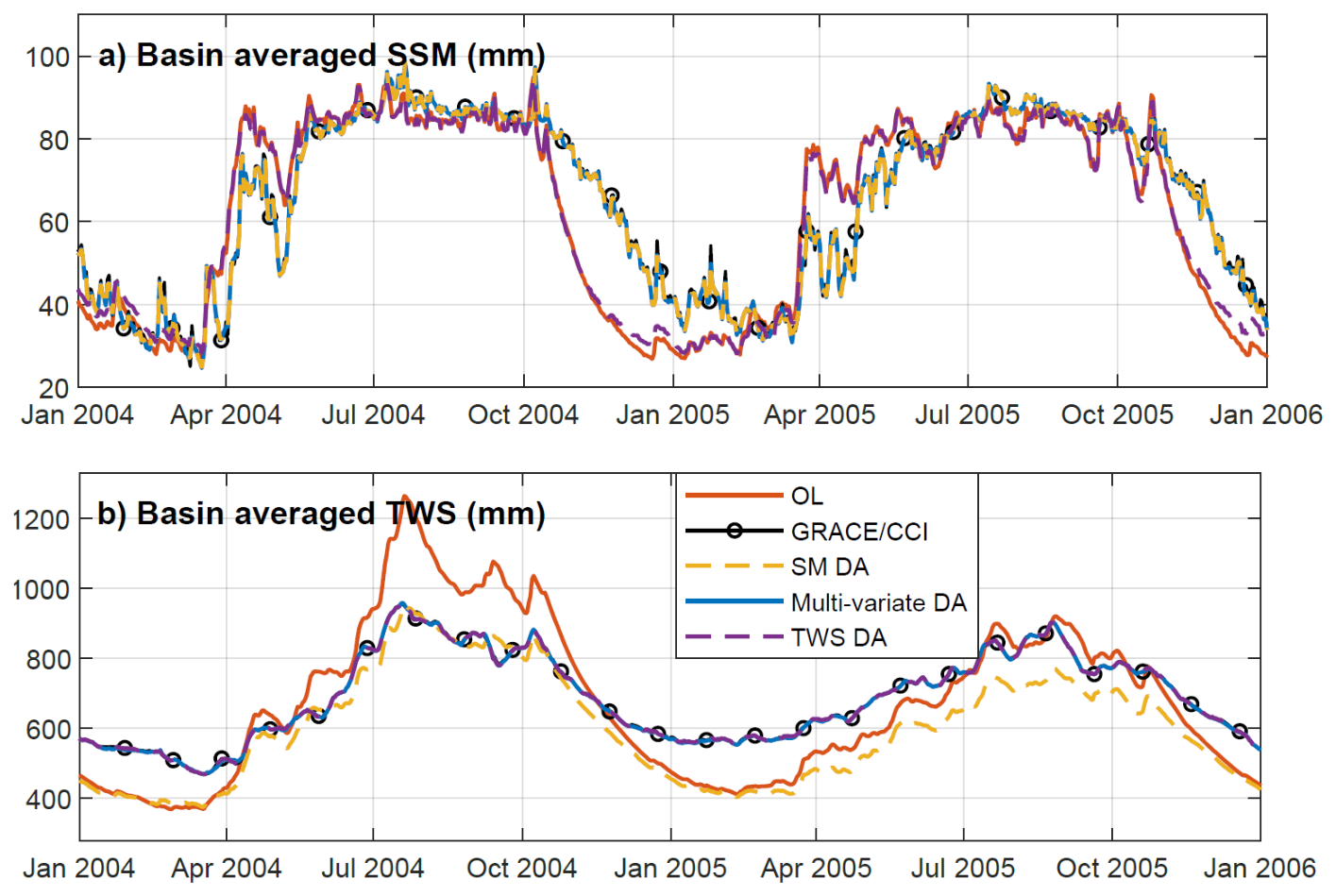
Figure B1 Impact of the different DA experiments on the sub-seasonal and sub-monthly variability of basin-averaged SSM (a) and TWS (b), for years 2004 and 2005.

Appendix C: Quantitative assessment of impact of DA settings on model estimates

Statistics of RMSD against assimilated data have been computed for the four DA tuning approaches considered in the main manuscript.

Additionally, the following plot shows the TWS times series of multi-variate DA with no DA tuning (approach #1). The time series reveal sharp spikes introduced by the SSM DA that are not observed in the GRACE TWS. The spikes are especially strong in the dryer periods (i.e., 2013–2015).

Table C1 RMSD of model estimates (OL, SSM DA, multi-variate DA and TWS DA) with respect to assimilated data. SSM min and SSM max refer to the minimum and maximum RMSD values across the 0.25°×0.25° tiles.

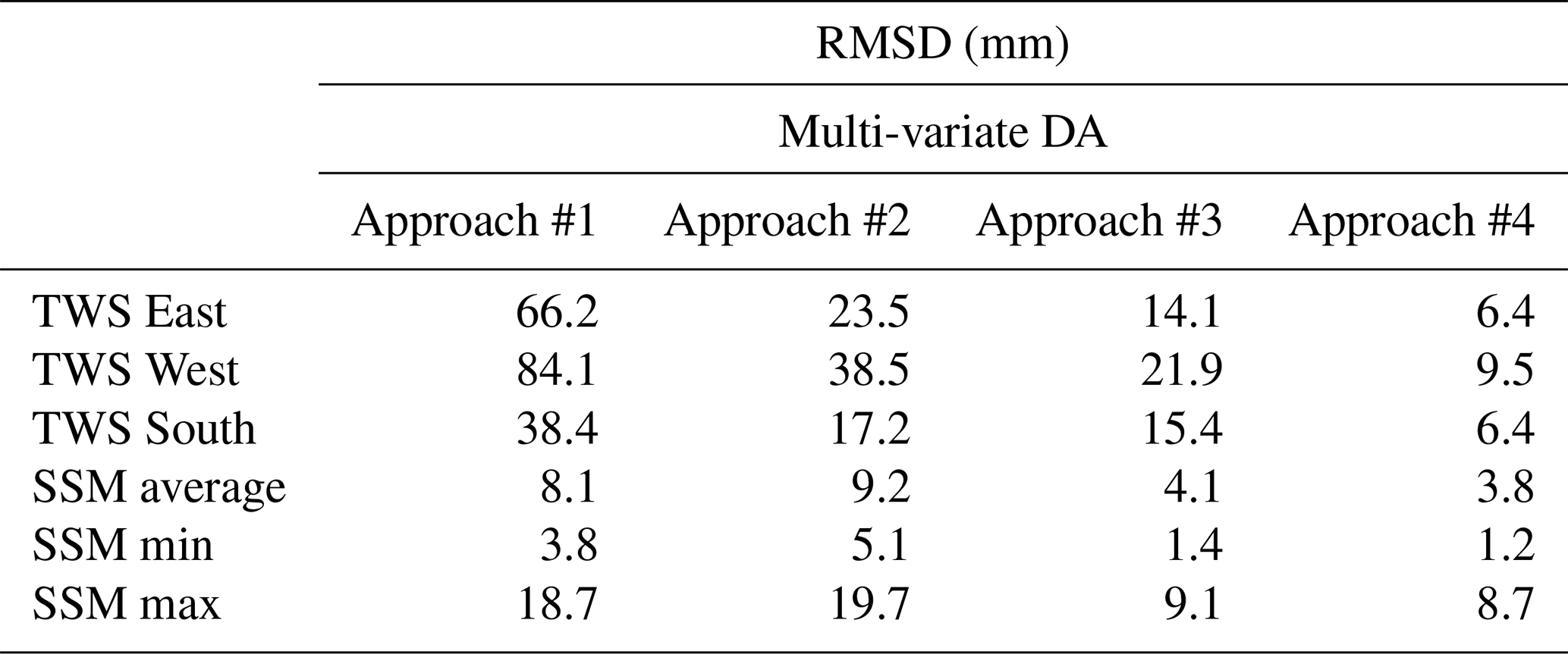
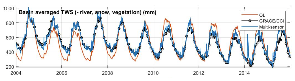
Figure C1 TWS time series for OL and multi-variate DA with no DA tuning approach. GRACE TWS is shown in black as a reference.

Appendix D: Evaluating the impact of additional DA setting parameters

In the main manuscript we evaluate the impact of localization and uncertainty adjustment settings on the multi-variate DA results. Here we present some additional results showing the sensitivity of the results to experimental settings such as groundwater localization degree, assimilation of detrended TWS and including river storage in the DA update process.

D1 Sensitivity of results to localization radius

Four additional multi-variate DA experiments were carried out to test the sensitivity of the results to different groundwater localization degrees. Half-radii of 0.5°, 4°, 20°, and no localization were considered, in addition to the 10° half-radius used for the experiments presented in the main manuscript. The SSM localization radii was kept fixed to 0.5° because it reflects the approximate resolution of the satellite observations (Sect. 3.1). The experiment was performed for the period 2003–2006.

The different localization settings reach a similar performance at assimilating the observations (not shown), but differ in the vertical and horizontal distribution of the DA updates (Fig. D1). Smaller groundwater localization radii (4° or 0.5°) produce sharp spatial patterns in the groundwater update which are likely not realistic. In contrast, when very broad groundwater localization radii are used (200° and no localization), we find an increased influence of TWS observations on the SSM component in the northern mountain areas (that is, areas where no SSM observations are available). The results are consistent with those reported in Retegui-Schiettekatte et al. (2025a), who suggest that the implementation of model space localization for TWS DA requires a compromise between excessively sharp spatial groundwater patterns and SSM degradation. The radius used in the main manuscript (100°) seems to offer a good compromise for this experiment.

It should be mentioned that the impact of the experiment with no groundwater localization on the SSM component is much lower than that found for the observation space localization setting in Sect. 4.2, as it does not modify the dynamics and decadal trends in the basin-scale. This confirms that model space localization can reduce the influence of TWS observations on SSM for areas where no SSM observations are available, but also suggest that it might not completely suppress this influence depending on the experimental setting.

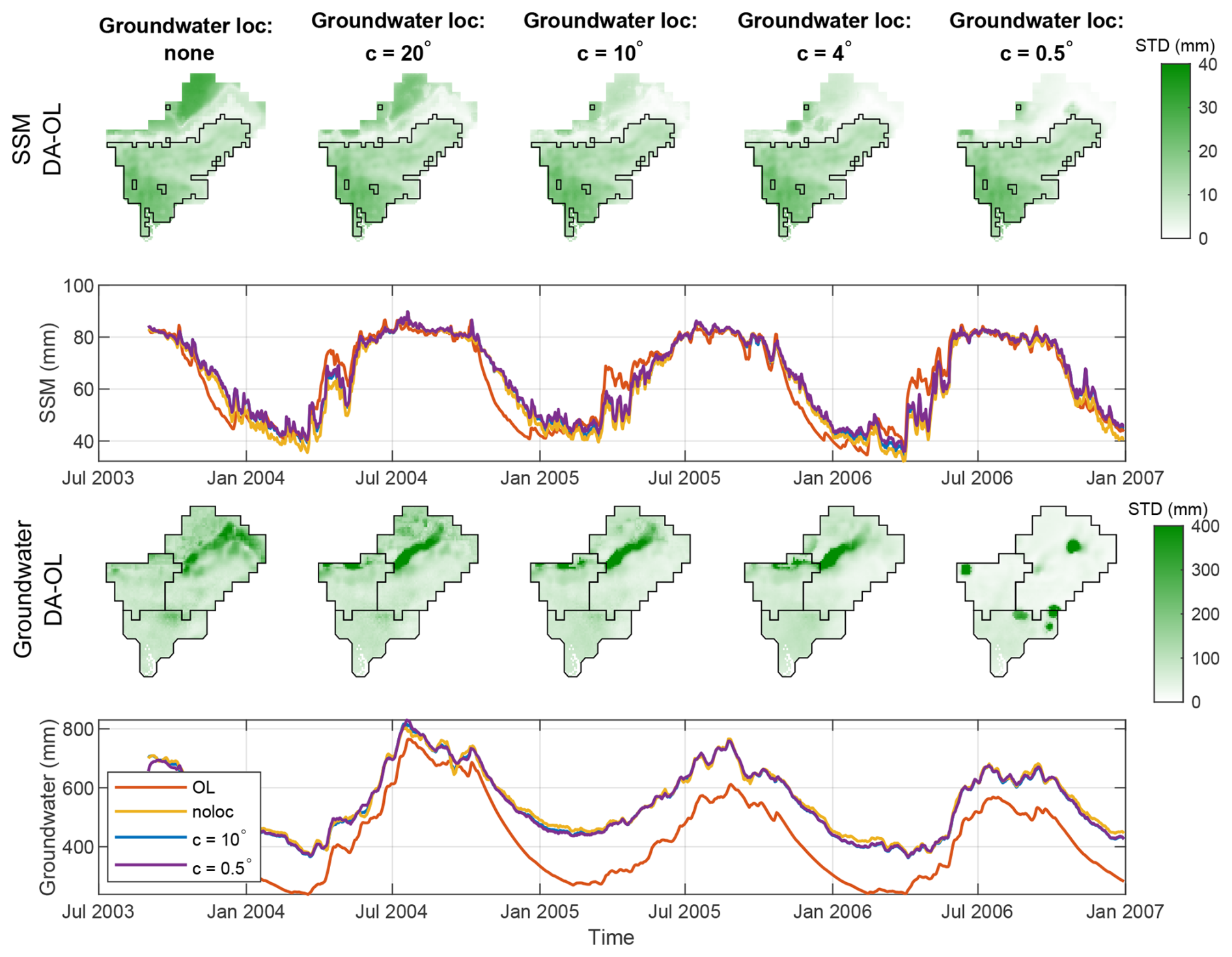
Figure D1 Standard deviation of DA minus OL on spatially distributed (0.1°×0.1° grid) model estimates for SSM (first row) and groundwater (third row) for different groundwater localization degrees. The standard deviation is expressed in mm. The plots in the second and fourth rows show time series for the same variables.

D2 Assimilating detrended TWS observations

Removal of glacier trends from TWS time series prior to the DA process was also implemented in a side-experiment. In general lines, the conclusions of the study do not vary when the trend is removed prior to DA. The results of the evaluation are summarized in what follows.

After multi-variate DA with prior trend removal, the RMSD difference between the modeled and assimilated observations is reduced below 10 mm, reaching values very similar to the experiments reported in the main manuscript with a maximum difference of 2.2 mm in RMSD between the two experiments. The vertical and horizontal disaggregation obtained when removing the glacier trends a priori are slightly different to those obtained when glacier trends were included, with stronger SSM updates in mountain areas where no SSM observations are available (similar to the results obtained with c=20° in Fig. D1). This could be suggesting that the “optimal” localization radius, that is, the one that limits impact on SSM while keeping realistic groundwater distribution patterns, might depend on the initial systematic differences between model and observations. Therefore, this “optimal” radius should likely be reconsidered when detrended TWS time series are assimilated, or when transferring this experimental setting to other regions.

The comparison of TWS estimates with SPEI leads to similar results as those presented in the main manuscript. The time series are very similar, and the statistics are identical for the West and South sub-basin and leads to a slight change of 0.04 correlation points in the East sub-basin. The improvement and degradation patterns in distributed groundwater estimates in the South sub-basin, where no glaciers impact is expected, were also found to be qualitatively similar. Some small differences were be found could due to the influence of in situ sites located close to the East sub-basin, where the prior removal of glacier trends in the assimilated data is likely to have an influence in groundwater updates.

The impact of the experiment in the SSM estimates is shown in Fig. F1, in terms of improvement in correlation coefficient with respect to WaterGAP SSM estimates. The improvements present a similar spatial distribution and intensity with respect to those represented in Fig. 9c of the main manuscript. Small differences can be observed along the northern edge of the area were SSM observations were assimilated (black outline in Fig. D2): the present experiment seems to slightly degrade SSM in this region, due to the increased influence of TWS on SSM estimates for this area. However, the degradation is not strong enough to significantly deteriorate sub-basin averaged SSM estimates, unlike the observation space localization results analyzed in Fig. 5c, g, k, m and o of the main manuscript, which lead to significant SSM degradations. Therefore, the degradations observed in Fig. D2 can be considered minor and do not seem to have a major impact on sub-basin averaged water storage dynamics.

Finally, the evaluation of river storage variability in the West and South sub-basin outlet indicates that a negative trend is introduced in the river storage time series, although the trend is less pronounced than that observed in the main manuscript (Fig. 10 of main manuscript) likely because the introduction of glacier trends in the groundwater component was avoided in this setting. As a summary, except for slight differences in some aspects including horizontal SSM update distribution and river water storage trends, the estimates obtained by removing the glacier trends prior to DA and after DA are overall very similar.

D3 Including river storage component in DA update process

Another alternative experiment was also performed by including the river storage component in the DA update process. For this experiment, the decadal trends were removed from the GRACE TWS time series to avoid transferring these into the river storage estimates. The validation was performed in terms of seasonal and sub-seasonal dynamics, and revealed that DA did not significantly improve river discharge time series (NSE of 0.84 and 0.84 for OL, and 0.86 and 0.88 for multi-variate DA, for the two sites represented in Fig. 1), but introduced notable noise in the sub-weekly timescale, which is especially visible in low flow periods in Fig. D3. Due to this reason, the river water storage component was excluded from the DA update process for the experiments presented in the main manuscript.

Additionally, it was already reported by Retegui-Schiettekatte et al. (2025a) (Fig. S8) that including the snow component in the update process can also introduce unrealistic anomalies in the snow estimates. Because of this, the two components were excluded from the DA update process in the experiments presented in the main manuscript.

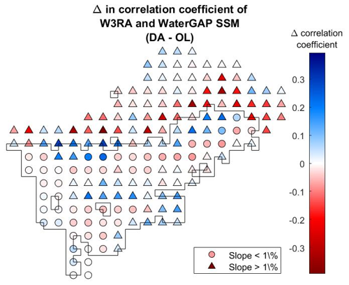
Figure D2 Distributed map of change in correlation coefficient between W3RA and WaterGAP after multi-variate DA when assimilating TWS observations without glacier trends. The black outline indicates the area where SSM observations were assimilated. This figure is analogous to Fig. 9c of the main manuscript.

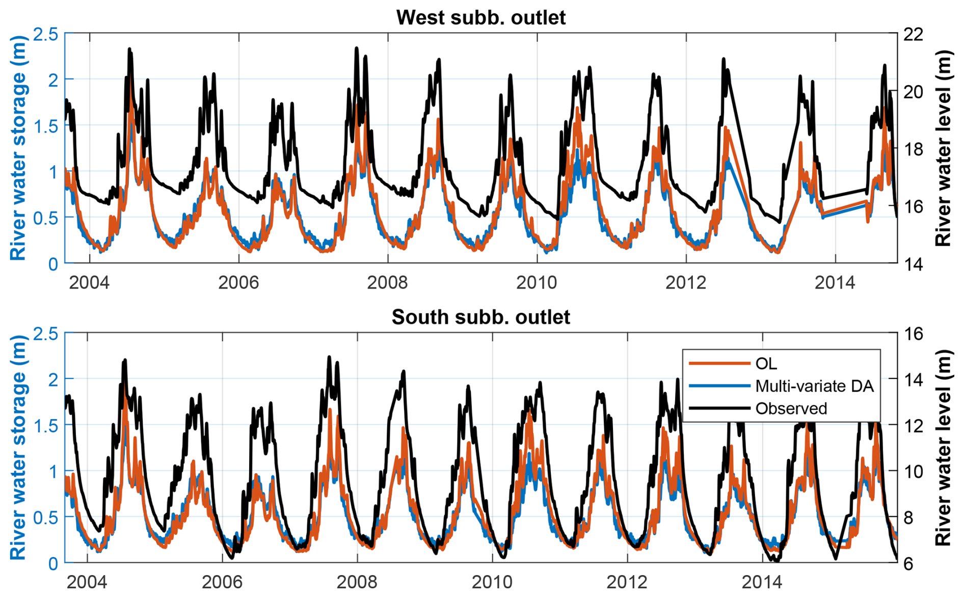
Figure D3 River water storage time series derived from OL (red) and multi-variate DA when river water storage is included in the state vector to be updated (blue), as well as in situ water level observations (black, with y axis on the right). The time series correspond to the two sites shown in Fig. 1.

Appendix E: Additional groundwater evaluation

Figure E1 reproduces the sub-basin averaged groundwater evaluation of the main manuscript while including the SSM DA and TWS DA experiment outputs. The results support the conclusions of Sect. 4.3.1 of the main manuscript that multi-variate DA fully captures the benefits of TWS DA on groundwater dynamics.

Figure E1 Inter-annual groundwater time series from OL, SSM DA, multi-variate DA and TWS DA experiments. In situ groundwater storage observations are shown for comparison (obtained with uniform specific yield, S_y=15, see Sect. 4.3.2).

Appendix F: Additional SSM evaluation

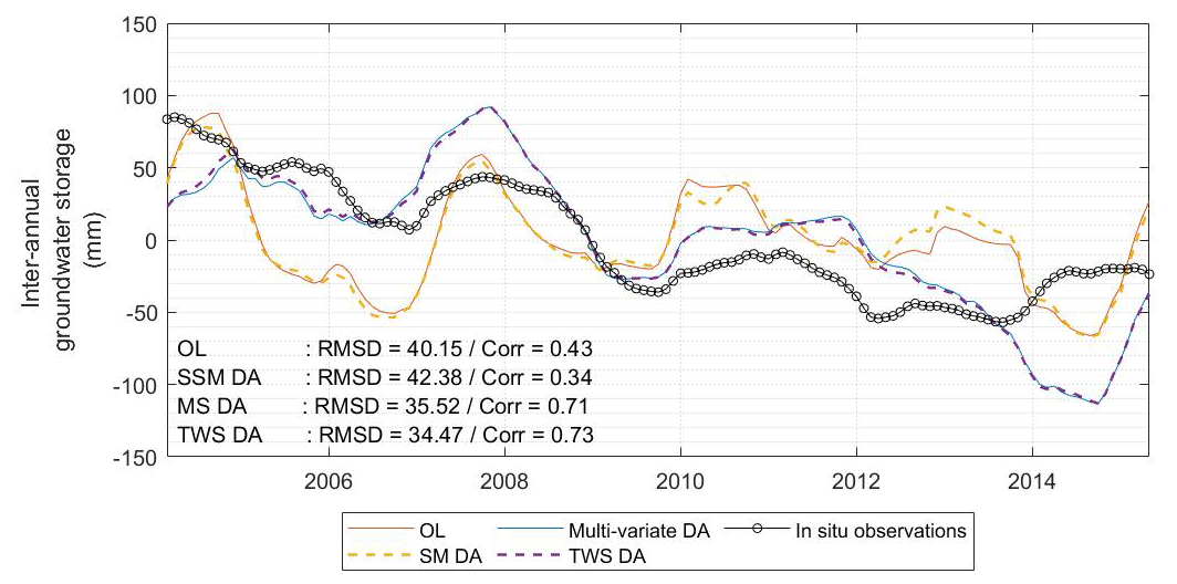
Differences between W3RA and WaterGAP SSM could originate from the difference in SSM layer depths. Indeed, the W3RA SSM average field capacity over the region is around 94 mm, while the WaterGAP average field capacity seems to be around 120 mm (see Fig. F1a). To exclude this possibility, we have repeated the comparison by considering all the soil water storage components of W3RA, that is, topsoil, shallow soil and deep soil, with an average field capacity of 452 mm over the region (see Table 2). The results still show that the W3RA SSM tends to saturate and decay earlier than the WaterGAP SSM (Fig. F1a) and present especially high discrepancies with WaterGAP in mountain areas (see Fig. F1b). This confirms that the differences might originate from the model structure rather than the SSM layer depth.

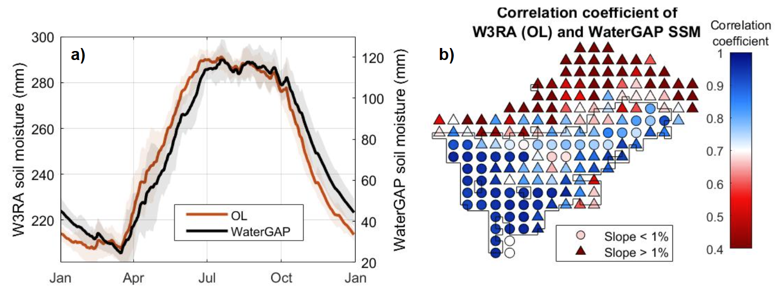
Figure F1 (a) SSM seasonality of W3RA OL (including deep soil) and WaterGAP. (b) Distributed map of correlation coefficient of W3RA (OL, including deep soil) and WaterGAP, shown for the WaterGAP 0.5°×0.5° tiles. The black outline in (b) indicates the area where SSM observations were assimilated.