Evaluation of SWOT HR PIXC version D water level time series of small lakes

The Surface Water and Ocean Topography (SWOT) satellite mission introduces unprecedented 2-D radar interferometry to inland hydrology, aiming to evaluate water bodies down to 0.0625 km². Standard operational products, such as LakeSP, are designed for global applicability but may exhibit suboptimal design choices for particular hydrological regimes. To address this, a customized processing workflow utilizing low-level SWOT L2 HR PIXC vD data was evaluated using 37 small Danish lakes (0.25 to 40 km²) against daily in-situ gauge data from July 2023 to May 2026. The workflow achieves a median root-mean-square error (RMSE) of 5.57 cm and a Pearson correlation coefficient (PCC) of 0.91, similar to LakeSP. Crucially, this approach retains a median of 125 valid timestamps per lake compared to 60 timestamps preserved by the filtered LakeSP product, effectively doubling the temporal resolution and enabling the capture of higher-frequency hydrological variations. Additionally, we find indications that SWOT's PIXC data contains time-varying residual roll-errors over Danish lakes that affect ca 18 % of all passes with more than 10 observed lakes covering Denmark.

1 Introduction

Continental water resources are affected by climate and, therefore, are important markers of climate change. In addition, human activities continue to impact rivers and lakes, potentially devastating biodiversity and human existence (Best, 2019). Therefore, it is crucial to continuously monitor the relative change in water surface elevation (WSE) of lakes and reservoirs worldwide to understand the underlying dynamics.

Traditionally, WSE is precisely measured by in-situ gauges, which can be expensive to install and maintain, and their data may not be public. In addition, the gauges are not evenly distributed across the Earth. Many lakes and rivers in remote areas and economically poor countries remain unobserved (Biancamaria et al., 2016). During the past 30 years, satellite altimetry has become an important, low-cost, freely available supplement in WSE monitoring (Abdalla et al., 2021). Globally distributed WSE time series are available from: Copernicus Land Monitoring Service (Copernicus, 2024), Hydroweb (Crétaux et al., 2011), “Database for Hydrological Time Series of Inland Waters (DAHITI)” (Schwatke et al., 2015), “USDA Lake Database” (Birkett et al., 2011), and “ESA CCI Lake ECV” (Carrea et al., 2024; ESA, 2024).

The launch of the Surface Water and Ocean Topography (SWOT) satellite mission in December 2022, led by the Centre National d'Études Spatiales (CNES) and National Aeronautics and Space Administration (NASA), represents a new era in satellite altimetry (Fu et al., 2024). It carries a dual-sided cross-track Ka-band Radar Interferometer (KaRIn) (JPL, 2024b), operating at 35.75 GHz (Biancamaria et al., 2016), with near nadir incidence angles (Fjørtoft et al., 2014). The KaRIn instrument enables SWOT to sense WSE within two 50 km wide swaths left and right of the satellite, separated by a 20 km wide nadir gap (Biancamaria et al., 2016; JPL, 2024b). The highest available resolution data product, the High Rate (HR) PIXel Cloud (PIXC), retains measurements outside the defined swaths (JPL, 2023b). This makes SWOT the first altimetry satellite to observe 2-D images of WSE. SWOT fundamentally transforms surface water hydrology by providing dense spatial sampling and temporally coherent observations of water surface slopes (WSS). SWOT operates in a 21 d repeat science orbit (cycle) (JPL, 2024b) with an average global revisit time of 11 d (JPL, 2024a). The majority of all lakes are located above 50° N (Lehner and Döll, 2004) which on average, will have at least 2–3 SWOT acquisitions per cycle (JPL/NASA, 2019; Biancamaria et al., 2016).

The unprecedented detail of SWOT data is expected to vastly improve our understanding of the dynamics of continental water bodies (Biancamaria et al., 2016) and, by extension, also of the Carbon (Cole et al., 1994) and Methane (Walter et al., 2007) budget. The dense spatial coverage enables studies of change at a regional scale, such as lake water storage, which is highly variable (Woolway et al., 2020). Importantly, with SWOT, the science objective is to monitor small lakes with an area down to 0.0625 km² (JPL, 2024b) – which represent a significant fraction of global lakes (Taburet et al., 2020) – that previously were too small to be observed by nadir satellite altimetry missions effectively. SWOT provides a more complete picture, enabling a better understanding and thus providing the basis for better decision-making.

Franze et al. (2025) investigate how SWOT can facilitate observations of the highly dynamic braided Brahmaputra river. Buzzanga et al. (2025) perform a case study on Death Valley, finding SWOT to measure water with unprecedented detail that will improve our understanding of freshwater availability and management in the future. Yu et al. (2024) compares SWOT RiverSP and LakeSP water surface elevations against Hydroweb and G-REALM product data, finding a good agreement, and Wigneron et al. (2024) validates the 1 d (calibration/validation) orbit RiverSP data against other satellite altimeters for river WSE, confirming good preliminary results, and highlighting the unprecedented spatial resolution SWOT provides. Jacobs et al. (2025) show that residual systematic errors in the SWOT data are detectable relative to nadir satellite altimeters over the ocean, anticipated by Peral and Esteban-Fernandez (2018).

This study investigates the feasibility of tracking lake-level anomalies in Denmark by constructing relative WSE time series from SWOT HR PIXC (version D) data. Using the SWOT LakeSP product as a baseline, we evaluate our workflow against in-situ gauge measurements from 37 lakes spanning a wide size gradient (0.25 to 40 km²). Through this evaluation, we aim to resolve two primary questions: first, how the utilization of lower-level data alters and potentially improves local lake-level monitoring relative to the standard LakeSP product; and second, whether residual roll errors remain identifiable in inland SWOT observations. Following this introduction, Sect. 2 details the data and study area, Sect. 3 describes the methodology, Sects. 4 and 5 present and discuss the findings, and Sect. 6 concludes the paper.

Initial investigations were done with the LakeSP product, but we found some issues for the small Danish lakes, where the WSE assignment to the PLD geometry resulted in assigning water to areas where no water is present. We have no reason to doubt the quality of the LakeSP product in other areas and expect it to improve over time.

2 Data and Study Area

2.1 SWOT

The joint CNES and NASA satellite SWOT was launched successfully on 16 December 2022 (used throughout this manuscript). It carries a Ka-band radar interferometer as the main scientific instrument. The SWOT mission aims to enhance our understanding of the global water cycle through measurements of ocean and inland surface water topography. It completed the initial calibration and test phase and has, since July 2023, been operating in its nominal 21 d science orbit (JPL, 2024b).

Inland water SWOT data is available in various products with different processing granularity. The most detailed information is available in the KaRIn water mask point cloud L2 HR PIXC data set (JPL, 2023b; SWOT, 2025b). In contrast, the L2 HR LakeSP product (JPL, 2023a; SWOT, 2025a) assigns and aggregates the PIXC data to lakes from the “prior lake database” (PLD) (Wang et al., 2023). River data is analogously available in the L2 HR RiverSP product (SWOT, 2025c). Here, we use the L2 HR PIXC data product version D as it provides the highest degree of freedom. From now on, we will refer to this dataset exclusively as PIXC.

SWOT sampling geometry is not uniform. The change of incidence angle across track is large, in relative terms, causing effective pixel spacings of ca. 60 to 10 m from close to far range (Fjørtoft et al., 2014). However, as noise levels increase toward the far-range, near-range observations provide higher data reliability. The along track resolution is fixed at 22 m (JPL, 2023b).

We use all PIXC data within 54.7–57.2° N and 8.1–12.6° E. File duplicates are identified by the Composite Release Identifier (CRID) and product counter. Since the lakes included in the study have a sufficient number of “open water” observations, we only use class 4 PIXC data, and not “water near land” (class 3). SWOT PIXC vD data up to cycle 50, pass 180 (16 May 2026) was used. We present prior LakeSP data from Hydrocron (Greguska et al., 2025) for comparison with our approach.

The LakeSP is filtered on the summary quality indicator “quality_f” =0 (zero is best), the flag determining the cross-over calibration quality “xovr_cal_q” =0 or 1 (meaning good and suspect), and the fraction of the lake's total area covered by dark water “dark_frac” ≤0.1 (JPL, 2023a). Where dark water is water with low backscatter typically representing lower quality measurements.

2.2 In-situ Gauges

In-situ stations measuring lake WSE are available through Vandportalen (WSP, 2024), combining multiple operator institutions. Most gauges cover the timeframe from the first SWOT 21 d science orbit cycle over Denmark (26 July 2023) up to date. The used gauge data has a daily resolution, and the water level is referenced to the Danish height system DVR90. To assess SWOT's ability to measure relative WSE change, we remove the median offset between SWOT and the gauge on a per-lake-basis, before reporting any metric. The offset for each gauge is listed in Table B1. The gauge uncertainty depends on the sensor. The water level is mainly measured with pressure and ultrasound sensors, where the uncertainty is listed as 15 and 5–30 mm (DMI, 2018).

2.3 Lake Geometries/Masks

The investigated lakes are exclusively located in Denmark and are selected from the lake (danish: “sø”) vector layer product of GeoDanmark (@geodanmark, 2024), documented in GeoDanmark (2018). The data set is updated cyclically every 5 years (KDS, 2024) and contains permanent lakes above 100 m² in surface area. Additionally, the set of lakes used in this study is truncated below a surface area of 0.25 km², leaving the 228 lakes, presented in Fig. 1. The lake geometries are used to extract the relevant PIXC data. The available lake information from GeoDanmark is manually expanded by: annotating lake names, indicating whether a lake possesses a gauge, the gauge's IDs, location, and vertical reference. In total, 37 gauged lakes are used in the comparison. Their surface area distribution is shown in Fig. A1D in the Appendix.

Figure 1 Map of Denmark with lakes larger than 0.25 km². Detailed list of all gauged lakes is provided in Table B1. Danish shapefiles from Klimadatastyrelsen (2026); @geodanmark (2024) and background borders from Sevdari and Marmullaku (2023).

3 Methods

3.1 Point Cloud Tile-Management and Masking

Lakes within one cycle and pass can be covered by multiple tiles. We, therefore, concatenate all tiles within one unique cycle and pass before further analysis. If a given SWOT pass partially covers lakes, we do not discard the affected lake from our analysis, as long as it fulfills the selection criteria described in the following subsections. The PIXC data product contains many targets that can have vastly different WSEs at proximity. To minimize their influence, we extract the PIXC observations via the lake mask.

3.2 Water Surface Elevation

The SWOT WSE with respect to the EGM2008 geoid used in this work (H_swot) is based on points with the “open water” class (JPL, 2023b) through the following expression

$$\begin{array}{}\text{(1)}& \begin{array}{rl}{H}_{\mathrm{swot}}\left(P\right)& =h\left(P\right)-\left(T_{\mathrm{solid}}+T_{\mathrm{load}}+T_{\mathrm{pole}}\right)\left(P\right)\\ & -N_{\mathrm{geoid}}\left(P\right),\end{array}\end{array}$$

for one point (P) with the natively reported height (h) given with respect to the WGS84 reference ellipsoid (JPL, 2024b), corrected for instrument and crossover calibrations, signal propagation delays due to iono- and troposphere (dry & wet) (JPL, 2023b), all three earth tides (T) as provided in the PIXC product, and the geoid height above the reference ellipsoid (N_geoid). Here we apply the EGM2008 geoid model (Pavlis et al., 2012) provided in the SWOT product. Danish lakes are rarely ice covered in the winter. We therefore chose not to account for potential ice cover.

3.3 Water Level Time Series: Data Selection Criteria

To account for outliers that persist after the spatial masking process, we utilise that SWOT surface elevations within one lake (on local spatial scales) are approximately normal-distributed. Therefore, an observation P (one point) is excluded if it is outside the 99.7 % confidence interval

$$\begin{array}{}\text{(2)}& H_{\mathrm{swot}}\left(P\right)\notin \left[\mathit{\mu }-\mathrm{3}\mathit{\sigma },\mathit{\mu }+\mathrm{3}\mathit{\sigma }\right]\left(H_{\mathrm{swot}}\right),\end{array}$$

with mean (μ) and standard deviation (σ) of the lake surface elevations H_swot for the respective acquisition. From this stage, we defined and tested six data selection criteria to understand which observation points should be used to summarize the WSE for the given timestamp. The criteria are presented in Table 1. We chose the median over the mean as the summary measure of the water level since it is more robust to outliers that might be missed by previous filtering. The median is applied to all points as filtered by the respective individual selection criterion (either all available points or points without a geo-flag). Where geo-flag refers to the point-wise 32 bit geolocation quality flag. In case of detected or suspected degradation the respective bits are turned to 1 according to Table 15 in the SWOT documentation (JPL, 2023b). It indicates the quality of variables such as elevation h, latitude, and longitude. We use the geolocation quality flag over the other available quality flags, as it is the designated quality flag for e.g. height in the SWOT documentation (JPL, 2023b).

The median WSE for a given timestamp and lake can be discarded based on WSE standard deviation, the number of points used for the median, or if too many points are geo-flagged. We found that acquisitions with fewer than 200 points produced outliers in the time series. We chose the threshold of 200 as an empirical threshold to balance retaining timestamps and removing outliers. Refer to Sect. 5 for further discussion. Generally, no lake is completely discarded based on the data selection criteria; it is strictly applied to the individual timestamps in the time series. Hence, if one lake's acquisition is discarded based on having fewer than 200 points, only that particular timestamp will be missing in the final time series. With this threshold, we deliberately accept less retained timestamps to trade off for “no” outliers in our timeseries. We do not perform weighting or spatial screening beyond the lake mask extraction. A flowchart of the method is shown in Fig. A1A in the Appendix.

Table 1 Data selection criteria describing how to aggregate one WSE measure for a given lake and timestamp, and when to discard it. With std: standard deviation.

3.4 Offset and Errors

The SWOT and gauge-based WSE time series have a constant offset, given the different vertical references. In addition, the SWOT KaRIn measurements are sensitive to errors in the roll angle and interferometric phase (JPL, 2024b), which are addressed in the satellite crossover calibration. Hence, potential errors in the crossover correction might introduce additional, time – varying errors between the gauge and SWOT – based water level time series, similarly to what has been shown for the ocean (Jacobs et al., 2025). Hence, if present, a remaining roll error at a given time stamp would result in a larger error, between the gauge and SWOT WSE in one side of the swath and a smaller one in the other side. Danish lakes typically have seasonal WSE variations of less than 1 m, thus, even minor remaining crossover correction errors would influence the time series. We see the possibility for a time-varying residual roll error (ϵ_roll) that is a function of the lake's position relative to the ground track of a SWOT pass – similarly to a “slope”. It could vary from pass to pass. SWOT error sources, in particular the roll error, are discussed in detail by Peral and Esteban-Fernandez (2018); Peral et al. (2024).

To report sensible metrics for relative WSE change, the constant offset per lake must be removed. The difference in WSE (ΔH) between the gauge (H_gauge) and SWOT is given by

$$\begin{array}{}\text{(3)}& \mathrm{\Delta }H(\mathrm{id},c,p)=H_{\mathrm{gauge}}(\mathrm{id},c,p)-H_{\mathrm{swot}}(\mathrm{id},c,p),\end{array}$$

with data for all cycles (c) and passes (p) for the respective lake (id), if gauge data is available and valid surface elevations H_swot following the selection criteria of Sect. 3.3 exist. The constant offset per lake (b₋) is then computed as

$$\begin{array}{}\text{(4)}& \begin{array}{rl}{b}_{-}\left(\mathrm{id}\right)& =\mathrm{median}\left(\mathrm{\Delta }H(\mathrm{id},c,p)\right),\\ & \Rightarrow \mathrm{\Delta }{H}^{\prime }=H_{\mathrm{gauge}}-b_{-}-H_{\mathrm{swot}}.\end{array}\end{array}$$

The roll error depends on the lake's distance to SWOT's ground track ($d\in [-\mathrm{60},\mathrm{60}]$ km). We use the lake's centroid and define negative distances to the left of SWOT's ground track. If roll errors are present, we expect a correlation between the gauge–SWOT difference ΔH^′ and the perpendicular ground track distance (d). We classify the acquisition to have a roll error if the correlation's p-value is ≤0.05 and if the ∣PCC$\mid \ge \mathrm{0.7}$. The error budget is superimposed with random noise ϵ_random for each lake. The total error is hence conceptually described as

$$\begin{array}{}\text{(5)}& \mathrm{\Delta }H(\mathrm{id},c,p)=b_{-}\left(\mathrm{id}\right)+d\cdot {\mathit{ϵ}}_{\mathrm{roll}}(c,p)+{\mathit{ϵ}}_{\mathrm{random}}(\mathrm{id},c,p).\end{array}$$

We expect the residual roll error to occur only in some of SWOT's acquisitions and to be small. We investigate indications of the error over Danish lakes, while the main focus remains on evaluating SWOT’s capability to detect relative WSE changes in small Danish lakes.

3.5 Statistical Evaluation with Gauges

The water level time series are evaluated per lake against gauge data. We are using the Root Mean Square Error (RMSE) and Pearson Correlation Coefficient (PCC) as performance metics. They are defined as:

$$\begin{array}{}\text{(6)}& \begin{array}{rl}& \mathrm{RMSE}=\sqrt{{\displaystyle \frac{\mathrm{1}}{N}}\sum {\left(x_i-y_i\right)}^{\mathrm{2}}},\\ & \mathrm{PCC}={\displaystyle \frac{\sum \left(x_i-\stackrel{\mathrm{‾}}{x}\right)\left(y_i-\stackrel{\mathrm{‾}}{y}\right)}{\sqrt{\sum {\left(x_i-\stackrel{\mathrm{‾}}{x}\right)}^{\mathrm{2}}\sum {\left(y_i-\stackrel{\mathrm{‾}}{y}\right)}^{\mathrm{2}}}}}\in \left[-\mathrm{1},\mathrm{1}\right],\end{array}\end{array}$$

with SWOT estimated water level (x), target offset removed gauge water level (y), and $\stackrel{\mathrm{‾}}{x}/\stackrel{\mathrm{‾}}{y}$ represent the mean. x is formed from H_swot, potentially with added corrections. Danish lakes typically have small seasonal signals (<1 m in 2023/24), deteriorating the expressiveness of the RMSE. Hence, it is important to consider both RMSE and correlation simultaneously.

4 Results

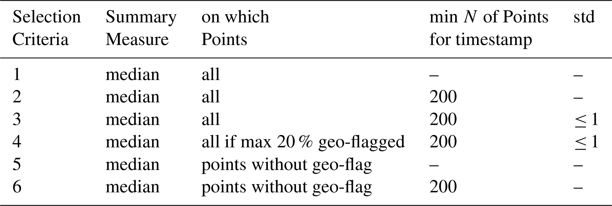
Figure 2 displays the time series for the six data selection criteria (Table 1) using Valsølille Sø, a representative Danish lake regarding surface area and seasonal signal. The figure includes the offset-removed gauge time series for criterion 6 as an example. Table 2 summarizes the performance metrics across all gauged lakes. Implementing a minimum threshold of 200 observations reduces the RMSE and increases the PCC, whereas the standard deviation threshold yields no metric improvement. Restricting geo-flagged points to a maximum of 20 % significantly improves both validation metrics, while completely excluding geo-flagged points yields similar performance. Criterion 6 performs equally to criterion 4 but contains no flagged points. Finally, the LakeSP time series exhibits strong RMSE and PCC values but retains significantly fewer valid timestamps than criterion 6. In the following, we utilized selection criterion 6. We present the development of the metrics over lake surface area from criterion 1 to 6 in the Appendix in Fig. A1B, C.

Figure 2 SWOT WSE time series for all 6 defined data selection criteria, exemplary for Valsølille Sø, with RMSE and Pearson Correlation Coefficient vs. gauge data and the number of timestamps in the respective time series (N). Filtered LakeSP prior data is shown for reference.

Table 2 Median and 2.5 % $/$ 97.5 % quantiles of the root mean square error (cm) and Pearson correlation coefficient [1] of all 37 used gauged lakes for the 6 time series data selection criteria. Summary metrics are described in Table 1, detailed lake specific metrics in Fig. B1.

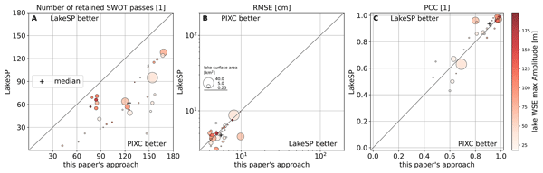
Figure 3 presents three offset-corrected water level time series alongside the corresponding LakeSP time series. Søby Sø (0.709 km² surface area, Fig. 3B) exhibits minimal WSE amplitude and a low correlation. Conversely, Tivolisøen (0.269 km² surface area, Fig. 3A) – the smallest gauged lake in this study – has a WSE amplitude exceeding 150 cm, an RMSE of 6.82 cm, and a PCC of 0.99. Mossø (16.569 km² surface area, Fig. 3C) represents a large lake in the Danish context and shows a low RMSE and a high SWOT-to-gauge correlation. Figure A1E displays a linear relationship in a gauge vs. SWOT scatter plot for Mossø. Our processing approach yields a median RMSE of 5.57 cm and a median PCC of 0.91 across all 37 gauged lakes. For comparison, the filtered LakeSP dataset achieves a median RMSE of 4.92 cm and a median PCC of 0.94. In contrast, filtered LakeSP retains a median of 60 timestamps over the nearly 3 years investigated, while our approach retains a median of 125 timestamps (mean: 62.8 vs. 118.9). Figure 4 shows the metrics and retained timestamps for our approach vs LakeSP against lake surface area and WSE amplitude. Table B1 lists the detailed metrics for all lakes.

Figure 3 Water surface elevation time series for three typical Danish lakes. Offset removed gauge data is shown in blue, our SWOT approach in red, and filtered SWOT LakeSP Prior time series are shown in the background for comparison. (A) shows Tivolisøen, the smallest lake in this study. (B) shows Søby Sø, a lake with minimal variation in water surface elevation. (C) shows Mossø, the third largest Danish lake.

Figure 4 Metrics and retained timestamps for this paper's approach and filtered LakeSP from Hydrocron. The circle size indicates lake surface area and the color indicated the maximum gauge WSE amplitude over the investigated timeframe.

At the latitude of Denmark, SWOT provides higher temporal resolution than most traditional satellite altimeters. Across the 228 Danish lakes exceeding 0.25 km², SWOT covers 54.63 % of the lakes with 4 passes per cycle, 22.47 % with 3, and 22.9 % with 2, yielding an average of 3.3 passes per cycle. After accounting for 42 inaccessible acquisitions out of 417, the effective temporal resolution averages approximately 9.5 d. Downsampling the in-situ gauge WSE time series to this 9 d resolution produces a median correlation coefficient of 0.96 (2.5 % $/$ 97.5 % quantiles: $\mathrm{0.63}/\mathrm{0.99}$) and explains 0.92 (2.5 % $/$ 97.5 % quantiles: $\mathrm{0.40}/\mathrm{0.99}$) of the observed variability.

4.1 Residual Roll Error

To address our second research question, if SWOT inland water data contains residual roll errors, we present Fig. 5A, which shows the height difference (ΔH^′) between the offset-removed gauge data and SWOT observations for lakes across all cycles of pass 152. SWOT observes up to 19 lakes in this pass, though data selection criteria reduce this number in individual cycles. This pass captures lakes in two hydrologically separate regions: blue markers designate lakes in Jutland, and red markers designate lakes outside Jutland. All lakes outside Jutland lie to the left of the SWOT ground track, whereas all but one Jutlandic lake lie to the right. While the ΔH^′ distribution across cycles generally centers around zero, certain cycles exhibit a slight offset. Gray bars highlight cycles with a significant roll component, where the ΔH^′ distributions for lakes in the right and left swaths differ considerably. Figure 5B–D plot ΔH^′ against the distance to the SWOT ground track for three specific cycles containing a significant roll component. The slope varies across cycles and reverses direction. We use the 1σ spread of the ΔH^′ distribution (shown in green) to quantify the roll error amplitude.

Figure 6A displays the SWOT-to-gauge error for all passes covering Denmark. Green and blue elements indicate the median ΔH^′ and 1σ quantile spread (84.15 %–15.85 %) for acquisitions with and without a significant roll error component, respectively. To minimize random effects, the plot only includes the median and quantile spread for acquisitions capturing at least 10 lakes. Out of 160 such acquisitions, 29 (approximately 18 %) exhibit a significant roll error component. Figure A1G and H shows ΔH^′ versus distance (d) for two acquisitions lacking a significant roll error; a slope is nevertheless visible. Figure 6B and D presents the median of the absolute ΔH^′ distribution for acquisitions with and without a significant roll error component; both medians remain close to each other for the investigated lakes. Figure 6C and E shows the distribution of the 1σ quantile ΔH^′ spread for these two categories, demonstrating a wider spread for acquisitions with a significant roll error. Aggregating these distributions yields a median $\mid \text{median}\left(\mathrm{\Delta }{H}^{\prime }\right)\mid$ of 1.79 cm. The spread across all acquisitions has a median of 5.43 cm and reaches 12.60 cm at the 0.95 quantile.

Figure 5 (A): ΔH^′ (SWOT vs. gauges) over time for all lakes in pass 152. (B)–(D): expanded plot of SWOT's error per lake over lake's centroid distance to SWOT's ground track. Negative distances are left and positive to the right of SWOT. Exemplary for the cycles 1, 17, and 36.

Figure 6 (A): ΔH^′ (SWOT vs. gauges) over time for all passes and all lakes in Denmark. For timestamps with ≥10 observed lakes, the median and 1σ quantile spread (0.1585 to 0.8415) are shown. If ΔH^′ significantly correlates with distance to SWOT's ground track (d), it is shown in green, otherwise in blue. The three vertical lines indicate the timestamps with detailed correlation plots in Fig. 5B–D. (B): distribution of the absolute median ΔH^′ for timestamps with significant roll error. (C): distribution of the 1σ quantile spread for timestamps with significant roll error. (D): distribution of the absolute median ΔH^′ for timestamps without significant roll error. (E): distribution of the 1σ quantile spread for timestamps without significant roll error.

5 Discussion

5.1 SWOT Sampling Geometry and Data

The cross-track variation in SWOT’s sampling geometry directly influences the operational performance of our 200 observation threshold. Because near-range pixel spacing is significantly larger (≈ 60 m) than far-range spacing (≈ 10 m), small lakes located in the near-range inherently yield fewer PIXC observations per pass, making the 200-point threshold harder to satisfy. Conversely, near-range observations benefit from lower noise levels and higher individual point reliability. While implementing an adaptive threshold based on a lake's cross-track position could potentially maximize temporal resolution, we chose to favor a uniform threshold to maintain pipeline simplicity and interpretability. Given that our uniform filtering approach already preserves a higher temporal resolution than the standard filtered LakeSP product, we think this choice is justified.

Similarly, our decision to restrict data extraction to the “open water” classification may limit analysis of small or narrow, elongated lakes, which naturally exhibit a higher proportion of “water near land” pixels. However, our results demonstrate that this constraint does not introduce a significant disadvantage at the spatial scales investigated in this study. For instance, Tivolisøen (the smallest gauged lake in this study, Fig. 3A) and Valsølille Sø (an irregularly shaped lake, Fig. 2) display robust performance metrics that align well with the overall median of the 37 investigated lakes, confirming the “open water” restriction to be viable for local lake level monitoring within our study's size and hydrologic domain.

5.2 Performance and Limitations

The aim of this study is to assess SWOT’s capability to capture relative changes in WSE in small Danish lakes, rather than absolute elevations. To derive the relevant metrics, we removed the median offset between SWOT and gauge measurements (b₋). This adjustment is sufficient for evaluating SWOT’s performance in detecting relative WSE changes. Consequently, investigating the origin of the removed offset lies beyond the scope of this study.

Criterion 6 matched the performance of criterion 4 while eliminating flagged data. We chose to adopt it as the more conservative selection strategy for this paper. By doing so, we aim to reflect the importance of producing accurate WSE measurements that are not contaminated by outliers. Our experiment's results highlight the critical trade-off between standard data products and customized lower-level processing. While the operational LakeSP product provides accurate WSE estimates with slightly better metrics, our filtering approach for the HR PIXC data preserves substantially more valid timestamps, thereby maximizing the temporal resolution necessary for robust local lake monitoring and other hydrologic applications. Especially for lakes with highly variable WSE patterns: even in Tivolisøen (Fig. 3A) peaks in WSE (November 2023 to February 2024; March to Mai 2024; January to March 2026) are completely missed by filtered LakeSP, but retained by our approach. This demonstrates that, despite similar metrics, our approach displays a clear advantage over LakeSP, given its higher temporal resolution.

While both our approach and the baseline LakeSP product aggregate WSE values from the SWOT PIXC product, two methodological choices separate the pipelines. First, LakeSP includes “dark water” and “water near land” pixels, whereas we restrict extraction strictly to the “open water” class. Second, LakeSP dynamically adapts the initial Prior Lake Database mask instead of utilizing a static mask. Specifically, “dark water” observations often carry higher noise levels, and the dynamic mask can inadvertently expand over shoreline features – such as wet soil – misclassified as water (Fig. B1F). By relying on a static mask and open-water pixels, our method circumvents these noise and misclassification pathways, reducing non-water artifacts and thus preserving a greater number of valid timestamps.

For global use cases or applications, where the temporal resolution is not of the highest priority, but ease of use and computational resources, we see LakeSP as preferable. Querying LakeSP from Hydrocron takes seconds per lake. Querying commuted lake level values from our approach from a local database is comparable to that. However, computing the PIXC data takes about one to two minutes per SWOT pass over Denmark – this has to be done only once.

In the presented timeseries (Fig. 3), the poor correlation observed at Søby Sø indicates that the lake's small WSE seasonal signal falls within the SWOT error budget. In contrast, the strong performance metrics at Tivolisøen demonstrate SWOT's capability to successfully monitor very small water bodies when they exhibit a high dynamic range. This shows, that a smaller lake surface area does not automatically result in worse mapping performance; the lake's annual hydrological amplitude must be considered concurrently.

The analysis on the temporal coverage of SWOT over Danish lakes highlights SWOT's capability to resolve the majority of WSE variations across the 37 studied lakes. While traditional missions like Sentinel-6 or Jason also achieve 10 d temporal resolution, their reliance on 1D ground tracks inherently limits the number of observable lakes. In contrast, SWOT's groundbreaking 2-D imaging capability allows it to monitor small lakes at high temporal frequencies that were previously unreachable. By successfully capturing these dynamics, SWOT advances our understanding of small lake hydrology and provides essential, high-resolution data to support water resource management for both policymakers and local communities.

5.3 Spatial Masking

A potential limitation of our proposed workflow concerns the reliance on a static water mask, as the resulting time series depend on the initial mask quality and the degree of seasonal variation in a lake's surface area. While Denmark features high-quality baseline masks and relatively stable lake extents, we evaluated this dependency by artificially expanding and shrinking the target lake polygons by 20 m. This buffer adjustment simulates both spatial uncertainties in the base mask and seasonal fluctuations in lake boundaries.

Modifying the polygons shifted the median RMSE from the baseline of 5.57 to 5.18 cm for the +20 m expansion and 5.02 cm for the −20 m contraction. The median PCC adjusted slightly from 0.91 to 0.92 in both scenarios, while the median number of retained timestamps remained nearly constant, moving from 125 to 126 and 125, respectively.

These minor variations suggest that the workflow is relatively insensitive to moderate boundary adjustments, indicating that a static mask may suffice despite spatial uncertainties or typical seasonal variations. This resilience likely demonstrates that SWOT's intrinsic water classification effectively excludes non-water pixels. Nevertheless, we suggest caution when applying a static mask to highly dynamic hydrological regimes, e.g. where lakes regularly dry out completely or double in surface area.

For such highly dynamic environments, users could incorporate a dynamic lake mask into the pipeline without encountering structural conflict. This modification would require a temporal matching routine to pair each SWOT acquisition with the closest available lake mask in time, while keeping a static mask as a fallback option. However, a notable downstream implication involves error propagation, as high spatial uncertainty within a dynamic mask can directly distort the aggregated WSE estimate. Excessively unstable masks, such as the example shown in Fig. A1F, could introduce significant error; therefore, we recommend that users only implement water masks they are confident in to prevent introducing artificial noise into the final time series.

5.4 Roll Error

The distinct geographical distribution of the Danish lakes relative to ground track 152 enables the clear detection of systematic spatial effects within the inland SWOT PIXC data. Lakes outside Jutland lie almost exclusively in the left swath and Jutlandic lakes largely occupy the right swath, a cross-track tilt manifests as a vertical discrepancy between the two regions. Based on the cases examined in Figs. 5 and 6, we observe temporal variations in both the magnitude and direction of this slope. As the sign of the slope varies between passes, we can rule out static reference surface issues, which would otherwise remain constant in time.

We are not trying to correct or quantify the residual roll error but only want to investigate its existence. Our set-up is not capable to robustly quantify it and perform an in-depth quantitative analysis of its amplitude. This is out of scope for our study and necessitates a dedicated research paper. However, our results clearly demonstrate its presence. Approximately 18 % of the acquisitions exhibit a tilting effect, suggesting that residual roll errors regularly affect inland SWOT data products. Crucially, while this roll component does not significantly alter the overall median error of a given pass, it degrades spatial precision by expanding the overall 1σ spread of the data distribution, with noticeable deviations appearing near the far-range edges of the swath.

Consequently, while researchers can likely ignore this effect for water bodies with large WSE variations, the tilt may influence the accuracy of WSE time series for lakes with small seasonal signals. More significantly, measurements of WSS could be superimposed with the residual roll error. Rivers perpendicular to a SWOT ground track would be particularly affected. We think, future SWOT users should maintain awareness of this potential error component. To mitigate this issue, researchers could estimate and correct for the tilt using linear approximations derived from gauge networks or virtual stations distributed across both swath sides. Ultimately, while future SWOT processing baselines will likely improve upon this issue, current applications require a deliberate choice on whether addressing this residual roll error for their respective use case.

5.5 Transferability

We established successfully, that our lower-level data approach can improve local lake level monitoring and that residual roll errors are present. To move beyond the circumstances of Danish lakes, we want to discuss in the following, how we foresee various environmental and geomorphological circumstances affect our processing pipeline.

Geomorphology impacts our approach in two distinct ways: first, tall flanking topography creates radar layover, which the SWOT intrinsic DEM masks, thereby reducing the number of valid observations per timestamp and potentially forcing our filter to reject lake observations that fall below the 200-observation threshold. Second, significant WSE differences along a lake's extent complicate the use of a single aggregated WSE value, introducing a sampling bias depending on where the lake was sampled by the retained SWOT pixels. While this effect remains negligible for small lakes, researchers likely should exclude extremely elongated lakes in mountainous terrain from this lower-level data approach.

Furthermore, seasonal frozen conditions alter surface properties, as ice cover degrades radar coherence, reducing the density of reliable observations and lowering overall data quality compared to open water, though the precise Ka-band scattering mechanisms over ice and snow warrant further investigation (Christoffersen et al., 2026).

Conversely, submerged vegetation and turbid water do not affect the WSE measurements because the Ka-band SAR signal does not penetrate the water surface, while surrounding canopy cover only blocks penetration along the immediate shoreline, functionally mirroring a slightly undersized lake polygon or the “water near land” class which we did not use in this paper.

Meteorological factors also modulate data quality, where wind conditions directly control radar backscatter intensity through an interplay of surface roughness, Ka-band wavelength, and satellite look angles; backscatter typically increases at wind speeds up to approximately 3 m s⁻¹ but decreases beyond this threshold (Fjørtoft et al., 2014), hence, in high wind regime environments, we expect worse data quality.

Changing hydrological regimes may impact SWOT measurements. The static lake mask could cause error by including land. However, we expect the impact to be small as we (i) use SWOT’s intrinsic water classification by using ‘open water’ only and (ii) using the median to aggregate a unified WSE measure per lake and time stamp – dampening the impact of outliers. We confirmed this in the mask expansion experiment. At the same time, if seasonal WSE signal is highly variable, higher temporal resolution increases in importance, which is where our approach retains more time stamps than filtered Lake SP.

Finally, regarding the transferability of our 200-observation threshold, heterogeneous shorelines affect our pipeline similarly to LakeSP but do not cause significant degradation when paired with an accurate lake mask. Using all 10 passes covering Denmark, our Danish lake dataset samples across the entire swath, hence cross-track positioning does not limit transferability; instead, we see steep terrain remaining as the primary operational bottleneck due to topographic observation loss. For applications targeting smaller lakes that intrinsically yield fewer pixels, users can easily adapt this pipeline by relaxing the 200-observation threshold or incorporating the “water near land” data classification.

6 Conclusions

This work demonstrates that lower-level SWOT HR PIXC data can be successfully leveraged to generate highly accurate relative water surface elevation (WSE) time series over small lakes. Based on a comprehensive validation baseline of 37 gauged lakes in Denmark evaluated from July 2023 to May 2026, our customized PIXC processing workflow captures relative WSE variations with a median RMSE of 5.57 cm and a PCC of 0.91. While the operational LakeSP product delivers a marginally lower median RMSE (4.92 cm), our approach offers a distinct advantage by retaining roughly twice as many valid observations (a median of 125 versus 60 timestamps). This significantly increased data retention preserves high-frequency hydrological variations that the standard products misses over Denmark. Consequently, future SWOT users should align their dataset selection with specific application requirements, carefully balancing operational simplicity against the desired temporal frequency of water level observations.

Additionally, we demonstrate the existence of a residual roll error in inland SWOT data, which affects approximately 18 % of the passes over Denmark. Although our experimental setup was not designed to robustly quantify the absolute amplitude of this error – warranting further dedicated research – SWOT users should remain aware of its presence and adapt their workflows accordingly. This artifact is particularly critical to consider when analyzing lakes with low hydrological amplitudes or when monitoring water surface slopes in rivers aligned perpendicular to the SWOT ground track.

The transferability of our approach beyond the specific hydroclimatic conditions of Denmark is feasible. Filtering thresholds can be adjusted and dynamic water masks can be integrated to accommodate more morphologically or hydrologically variable environments. Ultimately, SWOT provides unprecedented data, enabling the construction of high-temporal-resolution and high-accuracy WSE time series that were previously unattainable. This capability is especially impactful for small water bodies, many of which are now observed by a satellite altimeter for the first time due to SWOT's broad spatial coverage, which effectively overcomes the limitations of traditional nadir altimetry.

Appendix A: Supporting Figure

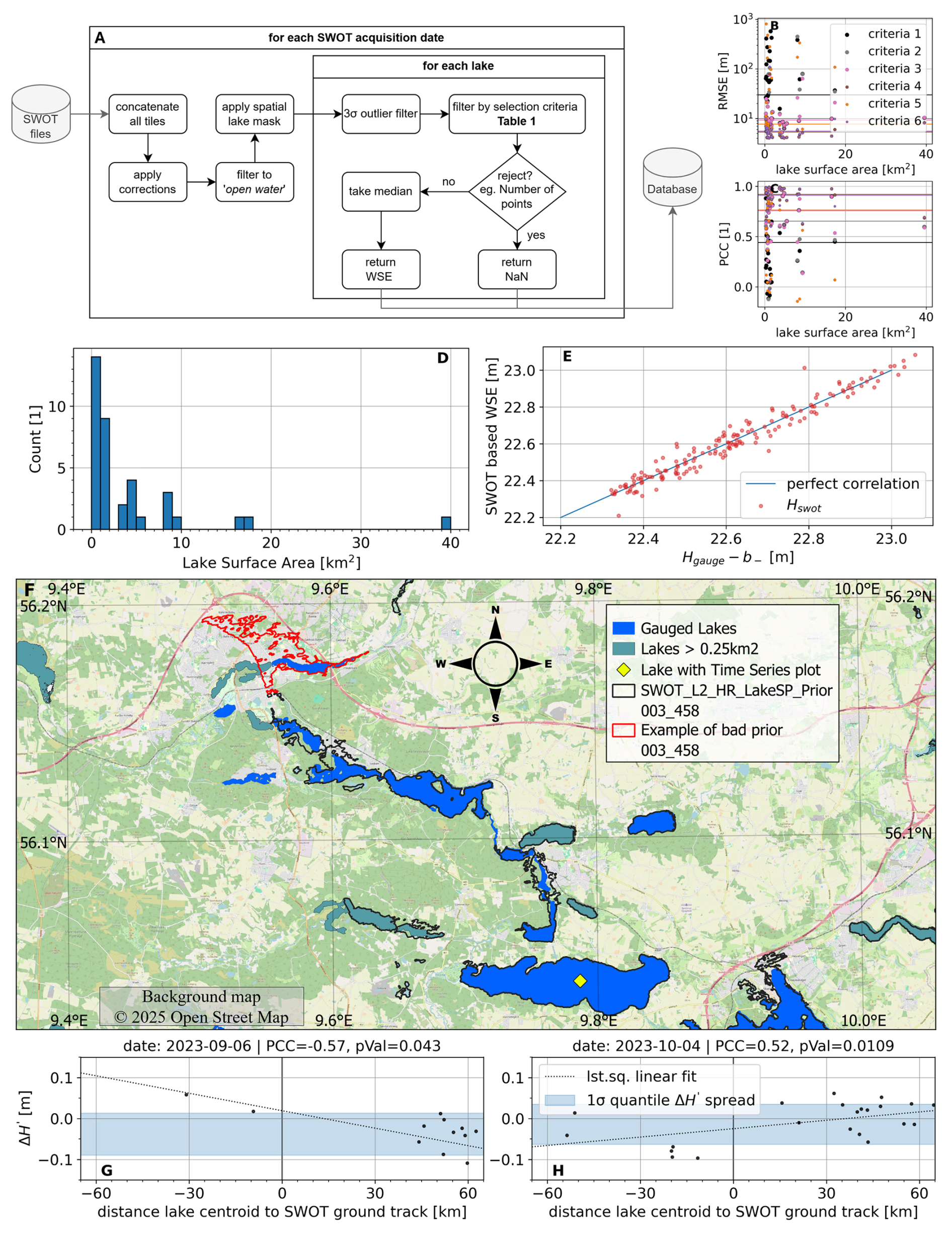
Figure A1 (A): flowchart of method pipeline. (B) and (C): RMSE and PCC for all lakes and all selection criteria over lake surface area. (D): distribution of lake surface area of all 37 lakes in this study. (E): correlation scatter plot for Mossø, shown in Fig. 3C. (F): Example of prior problem in LakeSP for Danish lakes around Viborg. (G) and (H): Example of two acquisition without significant residual roll error: error over distance to SWOT ground track.

Appendix B: Table of Gauged Lakes

Table B1 List of all used gauged Danish lakes (larger than 0.25 km²).

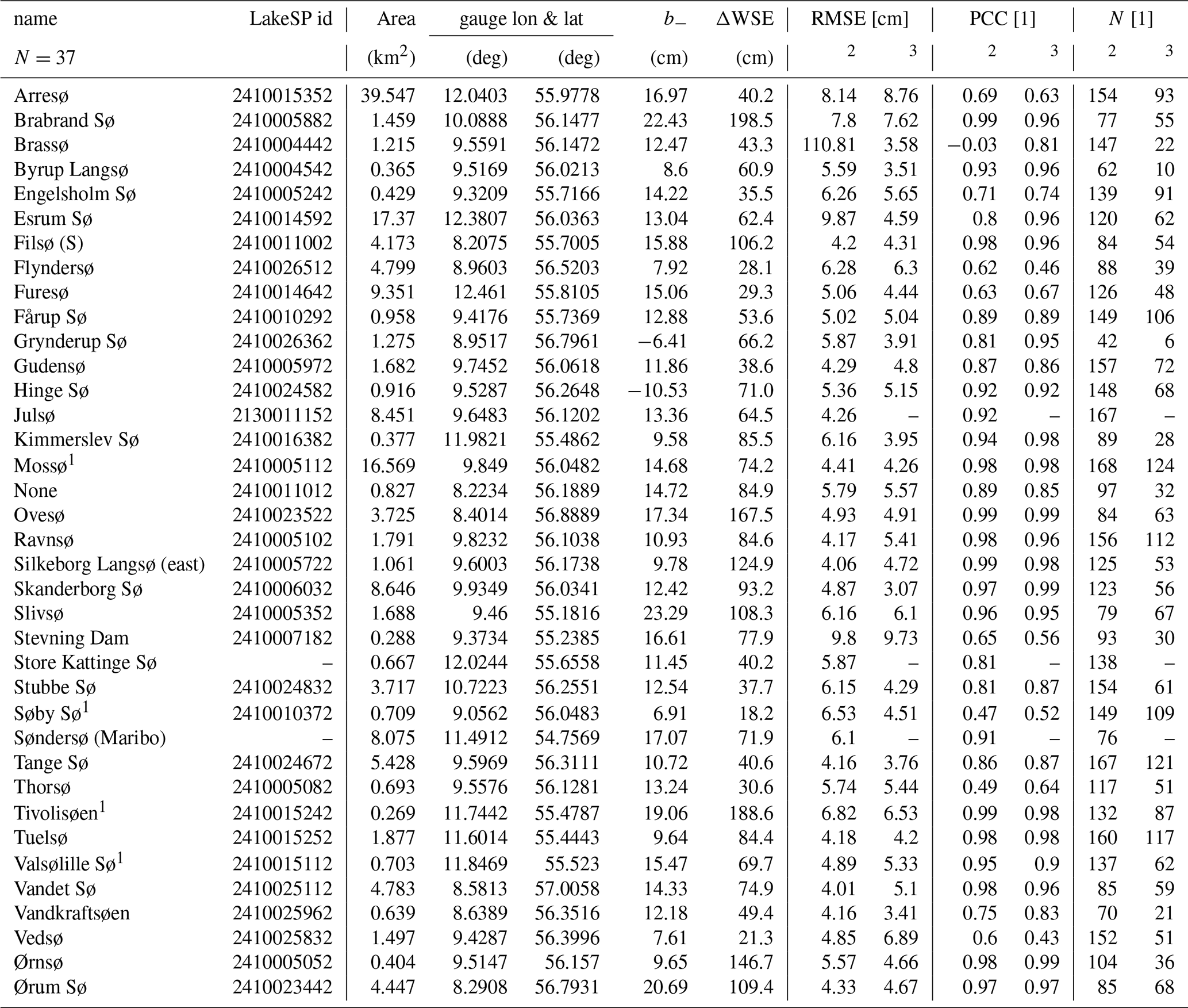
¹ Lake with time series plot. ² Relative metrics for H_swot (this paper's approach). ³ Relative metrics for LakeSP Prior (a dedicated offset is computed). b₋ Gauge offset wrt. H_swot. N: Number of SWOT based time series timestamps; for PIXC and LakeSP until 15 May 2026. ΔWSE: max. amplitude of WSE from gauge data.