Climatology and trends of observed daily and hourly extreme precipitation in the French Alps

The French Alps, characterised by complex topography and diverse climatic influences, are highly vulnerable to extreme precipitation events, which can trigger floods and landslides with significant socio-economic impacts. While local stakeholders report a perceived increase in sub-daily extreme precipitation events, such a trend has not yet been statistically confirmed based on observations. In this study, we apply extreme value theory to long time series of in situ observations of daily and hourly precipitation to provide an updated climatology and trend analysis of precipitation extremes across the region. We focus on 20-year return levels to analyse rare, potentially high-impact events and show that precipitation extremes exhibit distinct spatial patterns with marked differences between daily and hourly timescales. By examining trends at monthly and seasonal levels and making use of an existing weather pattern classification, we gain a deeper understanding of the dynamics underlying these trends. For extremes of daily precipitation intensity, we observe strong positive trends in the southern French Alps and negative trends in the north, primarily driven by a stronger influence of southerly (Mediterranean) flows in autumn. The spatial patterns for hourly extremes show more spatially variable trends, and seem to be primarily influenced by local thermodynamic effects potentially linked to e.g. changing moisture availability or changes in surface albedo due to shorter snow cover persistence. This detailed analysis provides important insights for stakeholders who are working on prevention and protection from precipitation-related hazards, underscoring the need for adaptive strategies in response to changing precipitation patterns. It also highlights the importance of region-specific and timescale-specific approaches in future studies of precipitation extremes.

1 Introduction

A direct consequence of global atmospheric warming is a profound modification of global atmospheric circulation and the entire climate system (IPCC, 2023). One of the main indicators of this change on a global scale is the intensification of the water cycle and an increase in hydrometeorological extremes, such as extreme precipitation and droughts (e.g. Markonis et al., 2019; Trenberth et al., 2003; Trenberth, 2011). Extreme rainfall, especially when it happens on very short timescales (minutes to hours), can lead to flash floods and landslides with important social and economic impacts. In 2024 alone, many such events hit the news, for example in eastern Spain, Nepal, Afghanistan or central Europe (WMO, 2025), which shows the urgency of better knowledge of probability and potential consequences of such events. Even southeastern France has not been spared from such events recently. In June 2024, intense rainfall at high altitude contributed to major flooding in the Ecrins massif (Blanc et al., 2024). In October 2024, locally more than 600 mm of rainfall in 48 h led to widespread flooding in the Ardèche province (Météo-France, 2024). And in May 2025, short but extremely intense thunderstorms (locally exceeding 120 mm h⁻¹ of precipitation) caused widespread damage in the southern Var province (Météo-France, 2025).

The French Alps are characterized by complex topography, which influences precipitation regimes and associated risks in various ways. First, the local relief induces significant spatial variability in orographically triggered precipitation (Kieffer-Weisse and Bois, 2001; Saidi-Bououdina, 1996). Second, steep slopes, especially when combined with unstable soils prone to erosion, are particularly exposed to landslides and flash floods (Creutin et al., 2022; Gaume et al., 2009; Llasat et al., 2016). These events can have catastrophic consequences when they affect homes, roads, or economic and touristic infrastructure. Third, the French Alps are located at the crossroads of Atlantic and Mediterranean climatic influences. A very clear climatic difference can be found between the northern and southern part of this region (e.g. Blanchard, 1921), which is also part of a larger climatic divide of the European Alps between temperate westerly and Mediterranean subtropical climate as found by Auer et al. (2007). While differences in topography, vegetation, and mean climatic influences can sharply define this divide, this may not be the case for extreme precipitation intensities. It should thus be regarded as a useful guide, not as a hard boundary. Indeed, previous studies have shown that for extremes the divide changes location over the seasons and over the years. For example, a study by Blanchet et al. (2021b) showed that the Mediterranean influence on precipitation extremes is weakening in winter and spring (DJF and MAM) in favour of the Atlantic influence, but strengthening in autumn (SON). With this background, both thermodynamic (a warmer atmosphere having a higher moisture holding capacity following the equation of Clausius-Clapeyron) and dynamic processes (changes in the relative influence of weather patterns) are likely to be of importance for assessing changes of precipitation extremes in our study region, thus complicating the big picture and the understanding of physical causes of trends (Jiang et al., 2023; Zeder and Fischer, 2020).

Previous studies, conducted primarily on daily precipitation extremes, have already shown trends in precipitation extremes in southeastern France in recent decades. For example, Ribes et al. (2019) used an approach that involved the analysis of a single time series of daily data, aggregated from several stations in southern France. They found an increase of precipitation with temperature one to three times larger than the increase in maximum moisture content of an air parcel with temperature (equation of Clausius-Clapeyron). They also noted that an increasing trend in annual daily precipitation maxima was non-existent until the 1990s and about 20 % to 40 % since then (until 2015). Blanchet et al. (2021a, 2016) found an increase in daily extreme precipitation in autumn (SON), particularly in the Mediterranean region, and a decrease in the northern Alps in winter (DJF). Studying the onset of statistically significant trends in daily precipitation extremes, Blanchet and Creutin (2022) showed that only in the 2000s did a coherent spatial pattern appear in sign and significance of trends in observations in southern France. In neighbouring Switzerland, Haruna et al. (2025) showed significant positive trends of extreme daily precipitation in the Swiss pre-Alps and the Swiss Plateau in winter, spring and summer (DJF, MAM, JJA) as well as in the southern cantons of Ticino and Grisons in autumn (SON).

Local stakeholders, working on prevention and protection from precipitation-related hazards, report a perceived recent increase in short-duration (< 24 h) but high-intensity precipitation in the French Alps, causing landslides and floods in areas where little or no such activity has been observed before (pers. comm. from stakeholders at RTM, EDF, Météo-France). However, to our knowledge, no studies have been conducted on possible sub-daily precipitation extremes in the French Alps yet. Given that in smaller catchments, changes in severe flooding intensity are closely related to changes in short-duration high-intensity precipitation events (Blöschl, 2022; Haslinger et al., 2025; Llasat et al., 2016) there is an urgent need to address this knowledge gap.

This type of small-scale precipitation events is usually caused by convective processes, typically thunderstorms. Regarding extremes, it is often assumed that in first order these should scale similarly with temperature as the potential increase in the water vapour content, which according to the Clausius-Clapeyron relationship is roughly 7 % K⁻¹ (Trenberth, 2011). As Fowler et al. (2021b) have shown in a literature review on hourly extremes, and John et al. (2022) in a model analysis studying daily extremes, in most cases studied so far this assumption seems to hold true, but locally scaling rates of two to three times higher have also been observed. Furthermore, it is generally observed that the trends in intensity should be higher for subhourly durations (Zheng et al., 2015; Dallan et al., 2022). While this has been found locally (Sydney, Australia: Ayat et al., 2022, Canada: Cannon et al., 2024) it is difficult to show on a global scale due to the very limited availability of long-term observations at such high temporal resolution. Both mechanistic and statistical explanations for such “super-CC” scaling rates at hourly and subhourly timesteps have been put forward (Fowler et al., 2021b, a; Loriaux et al., 2013; Da Silva and Haerter, 2025). Some studies (e.g. Loriaux et al., 2013; Fowler et al., 2021b) suggest that mechanistic reasons, i.e. an intensification of the convective system itself due to a non-linear response to an increase in temperature, are responsible for these “super-CC”-scaling rates. Other studies however, most notably an analysis by Da Silva and Haerter (2025) show that this might be a purely statistical effect, resulting from an increase of the convective fraction especially of mixed stratiform-convective systems. By splitting precipitation events into convective and stratiform they show that each of the two types individually scale very closely to CC-scaling. Yet another possible explanation, especially on local to regional scales, could be a shift in prevailing circulation patterns, i.e. atmospheric dynamics (e.g. Blanchet et al., 2021a).

There is no consensual definition of what characterises an “extreme”. Some authors study what we would term “heavy precipitation”, typically intensities above the 99th percentile or seasonal/annual maxima (thus exceeded between 3–4 times a year and every two years). Others, however, look at “extreme precipitation” as events that are rarely or never encountered in a human's life (e.g. return levels of 20 years or higher). In the present article we are mostly interested in the second class, as these events are likely to produce the strongest impacts. More precisely, we here define extremes as 20-year return levels. While studies of trends in extremes remain rare, a much larger body of literature provides insights into trends of heavy precipitation (e.g. Westra et al., 2013; Donat et al., 2016). Studies conducted in the European Alps (whole region: Menegoz et al., 2020, Switzerland: Bauer and Scherrer, 2024, Austria: Haslinger et al., 2025; Schröer and Kirchengast, 2018, northern Italy: Dallan et al., 2022; Giorgi et al., 2016; Brugnara and Maugeri, 2019) show how the complex interplay of synoptic patterns and local topography influences the spatial differences in trends in daily heavy precipitation (e.g. Bauer and Scherrer, 2024; Haslinger et al., 2025; Schröer and Kirchengast, 2018; Brugnara and Maugeri, 2019; Zeder and Fischer, 2020). Nevertheless, the European Alps as a whole show significantly positive trends in daily heavy precipitation (Menegoz et al., 2020). On sub-daily time scales, trends are generally positive and follow more closely the 7 % K⁻¹ relation expected from the Clausius-Clapeyron relationship (Haslinger et al., 2025; Schröer and Kirchengast, 2018; Dallan et al., 2022; Bauer and Scherrer, 2024). In summary, trends in heavy precipitation on daily timescales seem to be mostly influenced by changes in synoptic patterns, while short-duration high-intensity precipitation seems to be much more closely correlated to air temperature through dependency of moisture holding capacity and energy available for convection on air temperature (see also Giorgi et al., 2016). At this point it should also be mentioned that a study by Barbero et al. (2017) found overall less significant trends and lower temperature sensitivity of annual/seasonal maximum precipitation of hourly compared to daily precipitation over the contiguous United States, which is surprising given the widespread hypothesis of higher intensity trends for shorter durations. The authors attribute this to the more localised nature of high-intensity short-duration events, making them difficult to sample by ground-based rain gauge observations.

Even with the large body of literature on daily precipitation extremes and daily to hourly heavy precipitation in the European Alps summarised in the previous paragraphs, to our knowledge no study has analysed the trends of sub-daily extreme precipitation in the Alps, which is mostly due to the previously limited temporal depth and quality of available data. Many mechanical registrations of precipitation with high temporal resolution from pre-digital periods remain to be digitised, and digitally registered time series are only now becoming long enough to attempt an analysis of extreme precipitation trends on an hourly timescale, which is one of the main objectives of this study focusing on the French Alps. Previous studies of hourly precipitation extremes in the region have mainly focused on characterising spatial patterns and improving predictability. In the 1990s, the digitalisation of continuous observations (notably by Électricité de France, EDF, a French power company, as well as various other institutions) provided access to 30–40 years of data for about sixty stations, allowing the characterisation of extreme precipitation at sub-daily timescales (Garçon, 1993). This possibility was exploited in a series of doctoral theses at the time: Saidi-Bououdina (1996) studied the influence of local relief on precipitation extremes, showing for example that the influence of altitude on precipitation intensities is much smaller for hourly than for daily extremes. Kieffer-Weisse (1998) developed interpolation methods, and Djerboua (2001) worked mostly on the predictability of such extremes. Other methods of return level estimation exist and are applied operationally in e.g., SHYREG: Arnaud et al. (2016), but they are based on gridded datasets and/or stochastic precipitation generators, which are more indirect methods than the one we apply here and come with very different strengths and limitations. Today, with another 30 years of observations for many of the stations analysed in the previous studies by Saidi-Bououdina (1996), Kieffer-Weisse (1998), Djerboua (2001) as well as 25–30 years of hourly observations by the French national weather service Météo-France, we now have access to a much larger dataset of observations. With 163 stations having more than 25 years of observations (28 stations with more than 45 years, the longest with 71 years), we have a sufficiently large dataset to obtain updated estimates of return periods as well as, for the first time, studying trends of hourly extreme precipitation in the French Alps. Additionally, we build on and expand the work of Garavaglia et al. (2010) and Blanchet et al. (2016, 2021a) to get an idea of the weather patterns behind high-intensity precipitation in the region. Together with the estimates of return periods and their trends we thus aim to obtain an updated climatology of daily and hourly precipitation extremes in the French Alps.

The remainder of this article is organised as follows: Sect. 2 introduces the study area, the datasets used and the preprocessing steps applied. In Sect. 3 we outline the methodology. The results, including estimated stationary return levels, weather patterns associated to precipitation maxima, and trends of extremes are shown in Sect. 4. In Sect. 5 we discuss the results and then conclude the paper in Sect. 6.

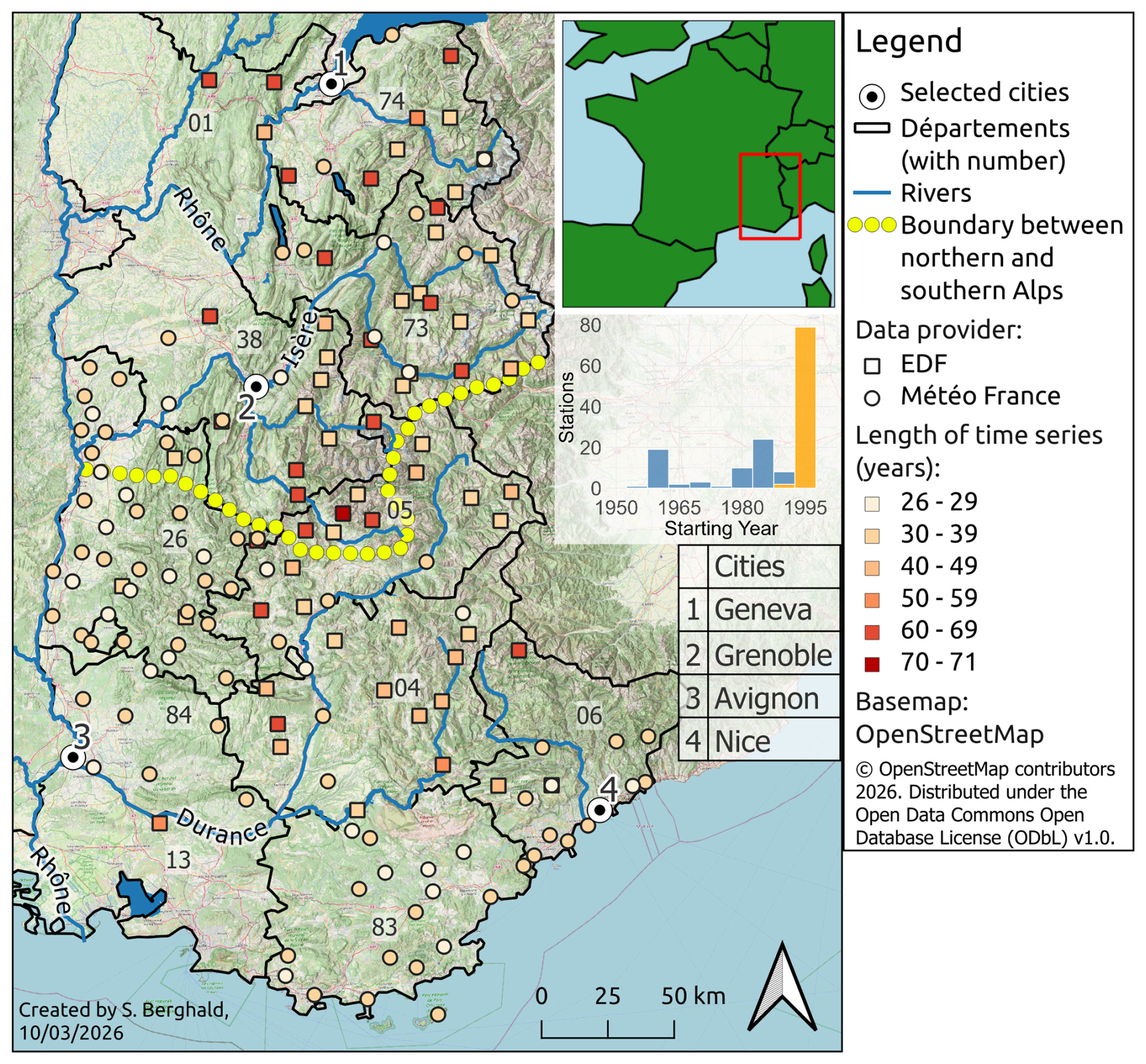
Figure 1 Study area and locations of precipitation observations used in this study. Stations maintained by Météo-France are shown as circles, and are used for stationary analysis only due to the comparatively short period they have been operating for. Stations maintained by EDF are shown as squares, and are used for both the stationary and the trend analysis (see Sect. 2.2.4). The colour of a point indicates the length of the hourly time series in years (including data from the “old” dataset where available). The length of daily time series is not shown, but frequently exceeds the length of hourly data. The boundaries of the administrative regions (départements) are shown in black with their respective codes (see text). Important rivers are indicated in blue, and selected cities as black dots. The yellow line shows the climatological boundary between northern and southern Alps (Blanchard, 1921; Auer et al., 2007). First inlet: Position of the study area within France. Second inlet: Distribution of starting years for all stations (blue: EDF, yellow: Météo-France). Basemap: © OpenStreetMap contributors, (2025), OpenStreetMap, hillshade: Esri (2025).

2 Study area and data

2.1 Study area

Our study area (shown in Fig. 1) covers the nine French départements (provinces) lying (at least partly) in the Alps. These are Savoie (official geographical code 73), Haute-Savoie (74), Isère (38) and Drôme (26) in the Auvergne-Rhône-Alpes region, as well as Hautes-Alpes (05), Alpes-de-Haute-Provence (04), Vaucluse (84), Var (83) and Alpes-Maritimes (06) in Provence-Alpes-Côte d'Azur. Due to their proximity, three stations in Ain (01) and one in Bouches-du-Rhône (13) are also included.

The French Alps are generally divided into two parts, characterized by different climatic influences (Blanchard, 1921; Auer et al., 2007). The division between the Northern Alps and the Southern Alps roughly follows a line passing through the mountain passes of Col de la Croix-Haute, Col Bayard, and Col du Lautaret, with the Écrins massif and its peaks reaching over 4000 m being the main meteorological divide between North and South (Fig. 1). The Northern Alps are generally higher than the Southern Alps and orographically very well structured: from west to east, there are first the pre-Alps (Chablais, Bornes, Bauges, Chartreuse, Vercors), followed by the central massifs (Mont Blanc, Beaufortain, Belledonne, Oisans, Pelvoux). Between the two lies the Alpine Furrow, a major north-south valley including the Grésivaudan and the Combe de Savoie valleys. To the east of the central massifs is the inner-Alpine zone, accessible via the upper Isère valley (Tarentaise), the Arc valley (Maurienne), and the Romanche valley.

The Southern Alps mainly consist of the Durance watershed with its tributaries Ubaye and Verdon. They are orographically less structured and generally lower in the outer areas (from Diois in the west to the Alpes-Maritimes in the south) and higher towards the Italian border in the east (Queyras and Mercantour).

The Northern Alps, under Atlantic influence, are among the rainiest regions in France with a mean precipitation of 1172 mm yr⁻¹ (June–August: 274 mm/3 months; mean values of our full dataset), while the Southern Alps experience a much drier Mediterranean climate (mean 855 mm yr⁻¹, JJA 144 mm/3 months) (Blanchard, 1921; Auer et al., 2007). The Atlantic influence in the north, with predominant westerly flows and the north-south orientation of the main mountain ranges, leads to very distinct climatic differences: the pre-Alps like Chablais or Chartreuse, being the first barrier for westerly flows, are characterized by high total precipitation amounts and comparatively low average temperatures. The Alpine Furrow, at low altitude and sheltered from westerly winds, experiences a mild and much drier climate. The central massifs then form a second barrier for westerly flows. This causes the inner-Alpine regions behind these mountain ranges, the Upper Tarentaise and Upper Maurienne, to experience a very dry, sunny, and continental climate. A particular climatic phenomenon in this region is the “East Return” which can locally bring very high precipitation amounts from the Italian Po valley and the Gulf of Genoa with humidity originating from the Mediterranean Sea (Garavaglia et al., 2010; Metzger, 2023).

The Southern Alps are characterized by a strong Mediterranean influence that decreases from south to north. Near the Mediterranean Sea, a strong seasonality between very dry summers and very rainy autumns can be observed. Precipitation intensities in autumn can locally be very high, with records exceeding 100 mm in one hour (Cannes, October 2015) and even exceeding 500 mm in 24 h (Saint-Martin-Vésubie, October 2020). Similar to the wider region of the north-western Mediterranean, autumn is also the season most prone to flooding in the southern Alps (Llasat et al., 2013), which is coherent with the climatology of extremes we present in this article. Outside the typical season for high-intensity precipitation, exceptionally extreme thunderstorms exceeding 120 mm h⁻¹ hit the coastal Var region in May 2025 (Météo-France, 2025).

2.2 Data

In this study, we use hourly and daily precipitation observations provided by Météo-France and EDF and a weather pattern classification described in Garavaglia et al. (2010). The datasets of EDF and Météo-France combined have time series for a total of 163 stations. In the following we give an overview over the datasets and the applied preprocessing steps.

2.2.1 Observations by Météo-France

The large-scale replacement of manually operated weather stations in France by automatised ones began in the late 1960s (Météo-France, 2020), but registration of precipitation at high temporal resolution (6 min intervals) was first introduced within the Météo-France network in the 1990s (Guillou, 2018). In 1996, Météo France decided to restructure, automate, and standardize its observation network with the launch of the RADOME project (Réseau d'Acquisition de Données et d'Observations Météorologiques Etendues; Tardieu and Leroy, 2003; Guillou, 2018). Quality-controlled data from this network is publicly available at meteo.data.gouv.fr (data.gouv.fr and Météo-France, 2023). We downloaded all available data until December 2023 included and selected all stations located in the study region for which at least 25 years of nearly complete (< 10 % missing data) precipitation observations were available between 1980 and 2023 (89 and 87 stations for hourly and daily observations respectively, circles in Fig. 1).

2.2.2 Observations by EDF

With the post-war onset of economic growth and thus rapidly increasing need for electricity, the French national electric power company EDF started to systematically assess and exploit the potential of hydropower in the French mountain ranges (Perret et al., 2012). As part of this assessment, an extensive monitoring network was established, featuring continuous observations of snow depth, river discharge and precipitation. Precipitation observations are taken since the 1950s using heated large-surface (2000 cm²) rain-gauges, with the precipitation rate registered by mechanic (past) or digital (today) tipping gauge. Current observations are registered hourly, and daily observations as the sum from 06:00 am until 06:00 am on the following day. Unfortunately, we were not able to reconstruct the evolution of the network with respect to the exact timing of modifications in the measurement devices. According to Garçon (1993), a change from mechanical to digital registration of observations took place in the 1980s, which seems plausible given that the datasets we obtained are structured very differently before and after this period. Recent data of 68 weather stations (squares in Fig. 1), covering the time from the 1980s to 2022, were made available by EDF for the purpose of our study. The dataset consists of daily and hourly data (68 stations), of which only the daily data is quality-controlled. For the hourly data, we employ a quality control procedure described in Sect. 2.2.3. One station was removed during this procedure, yielding now a total of 67 stations. For another station, the available hourly observations are too short for nonstationary analysis. We complete this “recent” dataset with an “old” dataset of digitalised observations covering the period from the late 1950s to the early 1980s (Garçon, 1993; Saidi-Bououdina, 1996; Kieffer-Weisse, 1998), and comprising 65 stations. Only weekly maximum precipitation totals for 1, 2, 3, 6, 12 and 24 h (fixed intervals, a day starting at 06:00 am) were archived and could be retrieved for our study. Of this old dataset, we use only observations for the 30 stations which are also included in the “recent” dataset. In summary, we have 30 EDF stations with weekly maxima for 1 h…24 h approximately covering the period 1955–2022 (squares with colours orange to red in Fig. 1) and another 37 stations covering approximately covering the period 1980–2022 (squares with colours yellow to orange).

2.2.3 Quality control of EDF observations

A quality control of the raw hourly data in the “recent” (since 1980) data by EDF was necessary. For this purpose, we used the quality-controlled daily data. The daily precipitation of a given day is the amount of precipitation that has accumulated in the 24 h between 06:00 am and 06:00 am of the following day. Should the sum of the 24 hourly measurements within this time span differ from the daily sum, we scale the hourly values, day by day, i.e. multiply each hourly measurement by a uniform factor, such that their 24 h sum from 06:00 am to 06:00 am on the next day equals the corresponding daily value. The relative distribution of hourly values during the 24 h remains unchanged in the process. Whenever the daily value is missing, or the difference between hourly sum (prior to scaling) and daily observation is too big (more than ±25 % of the daily value), all hourly observations of that day are set to invalid. Additionally, we visually inspected the seasonal distribution of maxima for each season and removed one station due to spuriously high maxima during the winter season (JFM) before 1980, resulting in a total of 67 stations in the dataset. For the old dataset no quality control could be done as only weekly maxima were available. Météo-France already does routine quality controls internally, we thus use their data as provided.

2.2.4 Datasets for stationary and trend analysis

From the datasets described above we use:

• For the stationary analysis: all observations covering at least 25 years in the period 1980 to 2023 for the 89 Météo-France stations (87 for hourly data) and the 67 EDF stations (i.e. 154 time series of both hourly and daily data, and 2 additional time series of daily data only), covering between 25 and 42 years of observations. While there are differences in instrumentation between EDF and Météo-France, we assume each individual time series to be homogeneous in time. Some of the EDF time series are combined from different datasets and thus may contain inhomogeneities between the first few years (early 1980s) and the rest of the period, which we consider negligible.

• For the trend analysis: 67 EDF stations (i.e. 66 time series of both hourly and daily data, and 1 additional time series of daily data only), covering between 34 and 71 years of observations between 1952 and 2022. At 30 of the stations, time series from different data sources are combined and thus contain known inhomogeneities from both changes in instrumentation and different quality control procedures before and after the 1980s.

2.2.5 Definition of seasons

During the initial analysis we found a clear shift in seasonality of extremes in the region: while the traditional way of defining meteorological seasons (winter: December–January–February) still seems most logical given just the stationary results, the monthly trends we find actually motivate a different definition (winter: January–February–March). We therefore decided to use this definition throughout the study.

2.2.6 Calculation of Monthly, Seasonal, and Annual Maxima

From the data obtained from Météo-France and EDF (and after correction of the latter), hourly and daily maximum values were calculated for each station, year, and month/season. According to the criterion proposed by Blanchet et al. (2016) and inspired by Papalexiou and Koutsoyiannis (2013), a maximum is considered missing if, for a given station, month/season, and year, its rank (ascending) is less than p_miss ⋅ N, with p_miss being the proportion of missing data and N the number of years of observations. For example, if a station has 30 years of observation and there are 20 % missing values for a given season/month, the value of that season/month is not taken into account if its rank is less than $\mathrm{0.2}\cdot \mathrm{30}=\mathrm{6}$. Thus, the more missing data points there are for a given season/month, the higher the maximum must be to be retained. For the old dataset just including weekly maxima, monthly maxima were computed by attributing weeks straddling two months to the months including the larger portion of the week.

2.2.7 Weather pattern classification

The weather patterns bringing precipitation to southern France can be classified into eight main classes, covering a range of generating flow condition modes over the Alps, the Massif Central, and the Pyrenees (Garavaglia et al., 2010, directions of flow shown in Fig. 2). These modes include three types of westerly oceanic flows (WP1 Atlantic Wave, WP2 Steady Oceanic, WP3 Southwest Circulation), three types of Mediterranean flows (WP4 South Circulation, WP6 East Return, WP7 Central Depression), Northeast Circulation (WP5), and Anticyclonic conditions (WP8). We here use the daily weather pattern (WP) classification by Garavaglia et al. (2010). In this dataset, which is regularly updated by EDF and thus includes the whole period covered in this study, each day is associated to one of the eight weather patterns, which for this day is thus the same for the whole region. Figure 2 shows qualitatively the evolution of the relative occurrence of each WP over time. Note that in the remainder of our study we group Atlantic (WP1,2,3) and Mediterranean (WP4,6,7) influences and thus obtain four different WPs. Following the method described in Blanchet et al. (2021a, b), we match each monthly maximum with the WP associated to that day. By doing so, we obtain series of binary variables, where $W_{t,m}=\mathrm{1}$ for a given weather pattern if it has generated the maximum of season or month m in year t, and 0 otherwise . In a stationary frame, we can then directly compute the relative contributions of the weather patterns to the total number of values for a given station. We call dominant with respect to a given month (season) the weather pattern that is associated with the largest number of monthly (seasonal) maxima over the complete time series at a given station.

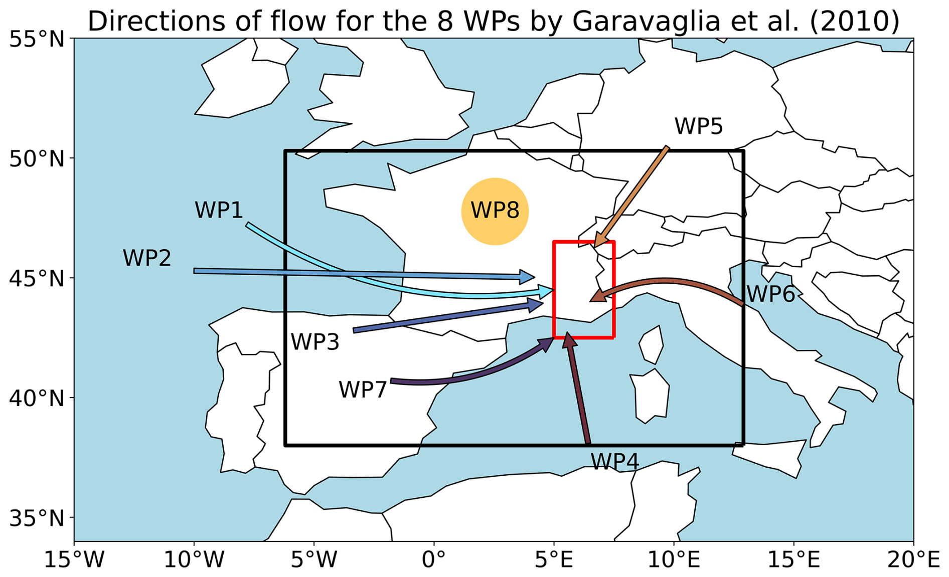
Figure 2 Direction of the large-scale flow directed to the study region for the eight weather patterns by Garavaglia et al. (2010) (WP8 groups anticyclonic conditions). The black box shows the area of interest for which the classification was done, and the red box shows the French Alps, the area of interest of this study. Figure adapted from Garavaglia et al. (2010, Fig. 3 therein).

3 Methods

We apply extreme value theory, based on block maxima (e.g., annual maxima) to characterise the climatology and trends of extreme precipitation in the French Alps. Our methodology is detailed in the following paragraphs.

3.1 Extreme Value Theory

3.1.1 Stationary GEV

For the estimation of return levels, we apply extreme value theory (Coles, 2001; Katz, 2013) based on the Fisher–Tippett–Gnedenko theorem (Coles, 2001; Fisher and Tippett, 1928) which states that for sufficiently large samples (e.g., daily precipitation sums for individual years), the largest or smallest value of each of these samples (e.g., annual maximum precipitation) follows one of three possible limiting distributions, which can all be summarised in the generalised extreme value (GEV) distribution. The GEV distribution is described by location ($\mathrm{-}\mathrm{\infty }<\mathit{\mu }<\mathrm{\infty }$), scale (σ>0), and shape ($\mathrm{-}\mathrm{\infty }<\mathit{\xi }<\mathrm{\infty }$) parameters:

$$\begin{array}{}\text{(1)}& \begin{array}{rl}P(X\le x)=& \exp \left[-{\left(\mathrm{1}+\mathit{\xi }{\displaystyle \frac{x-\mathit{\mu }}{\mathit{\sigma }}}\right)}^{-\frac{\mathrm{1}}{\mathit{\xi }}}\right],\\ & \text{ for }x\text{such that }\mathrm{1}+\mathit{\xi }{\displaystyle \frac{x-\mathit{\mu }}{\mathit{\sigma }}}>\mathrm{0}\end{array}\end{array}$$

A special case is ξ→0, which gives the Gumbel distribution (Coles, 2001):

$$\begin{array}{}\text{(2)}& P(X\le x)=\exp \left\{-\exp \left[-\left({\displaystyle \frac{x-\mathit{\mu }}{\mathit{\sigma }}}\right)\right]\right\}.\end{array}$$

The quantiles of the distribution can now be obtained by transforming Eqs. (1) or (2):

$$\begin{array}{}\text{(3)}& x_p=\left\{\begin{array}{ll}\mathit{\mu }-\frac{\mathit{\sigma }}{\mathit{\xi }}(\mathrm{1}-\mathit{\{}-\log (\mathrm{1}-p){\mathit{\}}}^{-\mathit{\xi }}),& \text{if }\mathit{\xi }\ne \mathrm{0}\\ \mathit{\mu }-\mathit{\sigma }\log (-\log (\mathrm{1}-p\left)\right),& \text{if }\mathit{\xi }\to \mathrm{0}\end{array}\right.\end{array}$$

where x_p is the return level corresponding to the return period p⁻¹ (e.g. $p=\frac{\mathrm{1}}{\mathrm{20}}$ for a return period of 20 years).

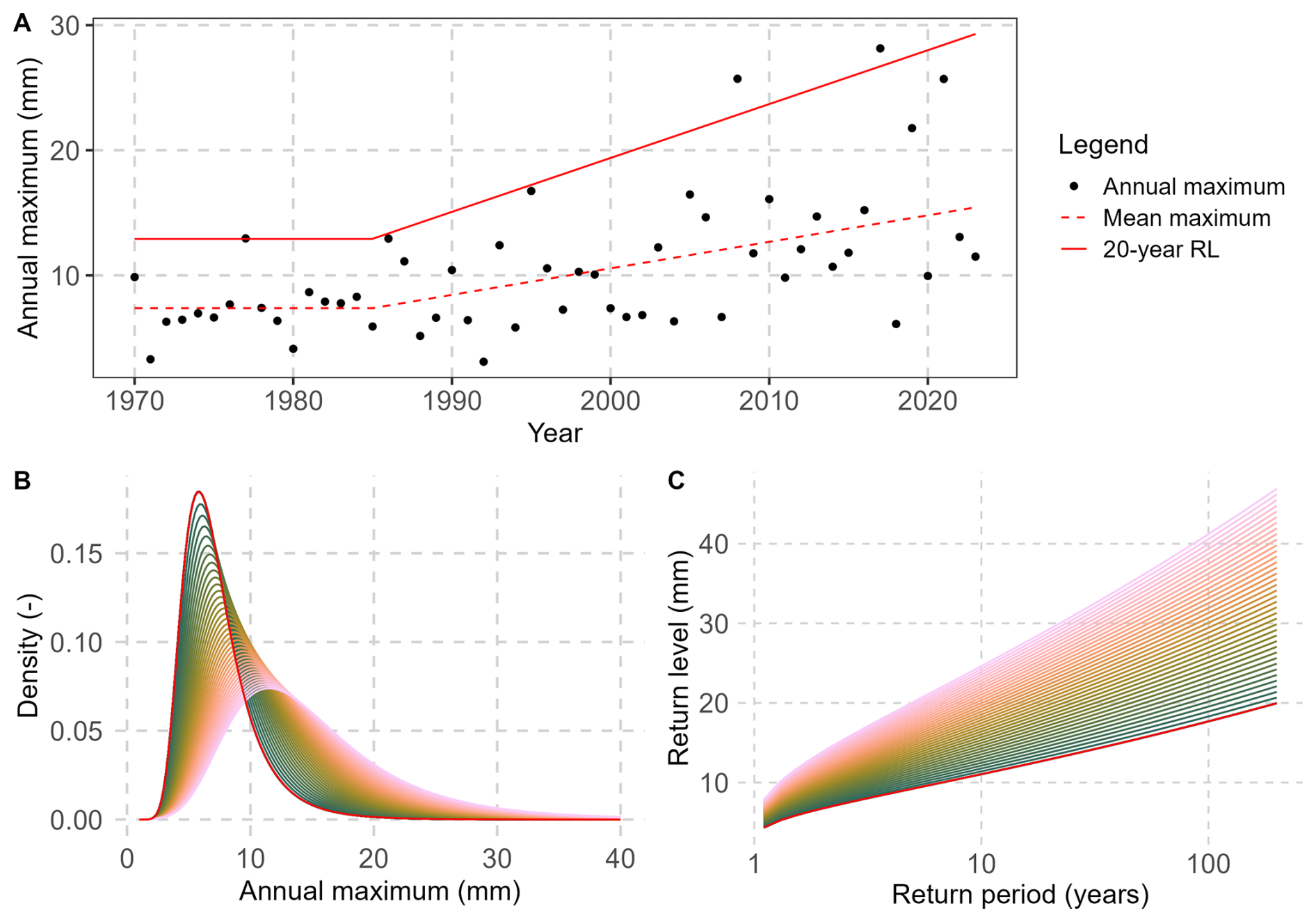
Figure 3 (A) Idealised time series of annual maxima with a linear trend in location (μ) and scale (σ) parameters after the year 1985 including mean maximum (red, dashed) and 20 year return levels (red, solid). (B) Associated GEV density plot for each year between 1970–1985 (stationary, red) and 1986–2023 (green to pink). (C) Associated return level plot.

We consider GEV distributions for three block lengths: monthly, seasonal, and annual maxima. Three potential limitations can be mentioned: first, the values in each sample (e.g. year) must be independent and identically distributed. The latter assumption could be violated if block maxima at a given location were generated by different precipitation processes. As we discuss in Sect. 5.1.3 this is actually not the case in our study region, even for annual maxima. Second, extreme value theory is an asymptotic theory where the block length is assumed to be almost infinite. This is clearly not the case in any application, and even less for monthly maxima. Nevertheless, the obtained GEV distributions fit reasonably well their corresponding series of maxima on return level plots (not shown). Lastly, it could be argued that fitting a GEV to seasonal or annual maxima could be incoherent compared to obtaining seasonal or annual return levels from the monthly GEV distributions (by multiplying them, see e.g. Carter and Challenor, 1981). However, in our experience multiplying GEV distributions entrains, in some cases, strong biases due to error propagation, and is therefore not a good option for our dataset. This is further discussed and illustrated in Sect. 5.1.3.

3.1.2 Non-stationary GEV

Non-stationarity is included in this concept by allowing one or more parameters of the distribution to vary with a covariate (Katz, 2013). Here we use time (in years) as covariate and redefine parameters μ and σ such that they remain constant until a breakpoint year (1985), after which they evolve linearly. This breakpoint is motivated by several considerations: (i) previous studies have shown that statistically significant trends of daily precipitation extremes in southern France start in the 1980s (e.g. Blanchet et al., 2016), (ii) this is also the time where the old dataset including only weekly maxima ends and we start to have the raw hourly observations available, and (iii) most likely, a change in instrumentation took place in the 1980s and/or early 1990s, switching from mechanical to digital registrations. Using a breakpoint, we are able to minimise potential biases stemming from the different lengths of observations while being able to take the additional data previous to 1985 into account to make the estimations more robust. Here it should be recalled that for the non-stationary analysis we use only EDF time series.

Consequently, we define the non-stationary model ℳ_μ,σ such that the linear trend starts in 1985, with stationarity before that year:

$$\begin{array}{}\text{(4)}& \left(M_{\mathit{\mu },\mathit{\sigma }}\right)\left\{\begin{array}{l}\mathit{\mu }\left(t\right)=\left\{\begin{array}{ll}{\mathit{\mu }}_{\mathrm{0}},& \text{if }t\le \mathrm{1985},\\ {\mathit{\mu }}_{\mathrm{0}}+{\mathit{\mu }}_{\mathrm{1}}(t-\mathrm{1985}),& \text{if }t>\mathrm{1985},\end{array}\right.\\ \mathit{\sigma }\left(t\right)=\left\{\begin{array}{ll}{\mathit{\sigma }}_{\mathrm{0}},& \text{if }t\le \mathrm{1985},\\ {\mathit{\sigma }}_{\mathrm{0}}+{\mathit{\sigma }}_{\mathrm{1}}(t-\mathrm{1985}),& \text{if }t>\mathrm{1985},\end{array}\right.\\ \mathit{\xi }\end{array}\right.\end{array}$$

Because of the difficulties associated with estimating the shape parameter ξ, we choose to keep ξ constant, which is common in the literature (Katz, 2013; Jayaweera and al., 2025; Salas and Obeysekera, 2014). Figure 3 shows the influence of a linear trend in μ and σ starting in 1985 on an idealised time series of maxima, on the density of the GEV distribution, and on the corresponding return periods. Submodels M_μ (trend only in μ) and M_σ (trend only in σ) are also considered to account for cases when the whole density curve of maxima shifts in time (M_μ), or when only the variability of maxima changes (M_σ). We then select at each station the best non-stationary model among M_μ, M_σ and M_μ,σ as the one minimizing the Akaike information criterion (AIC, Akaike, 1974). Finally, we derive from the selected model the evolution in 20-year return levels, using Eq. (3) (red solid line in Fig. 3A). The choice to focus in this study on the 20-year return level is arbitrary; it aims at documenting changes in very rare events that are encountered only a few times in a human's lifetime. Spatial patterns associated with 10-year and 50-year return levels are not shown but have similar patterns.

To assess the significance of changes in 20-year return levels, we adopt a bootstrap approach by resampling the series of maxima 500 times with replacement, fitting the best non-stationary model to each resample, and looking if the 5 %–95 % confidence interval of 20-year return level changes includes zero, in which case we consider the change not significant. We prefer this method over the classical likelihood ratio test (Coles, 2001) as it specifically evaluates changes in the extremes (20-year return levels). In contrast, the likelihood ratio test assesses whether the entire distribution has changed, which could also indicate changes in heavy precipitation (e.g. in mean maxima) rather than in the extremes.

3.2 Parameter Estimation

3.2.1 Theory

In the nonstationary case, parameters are estimated using maximum likelihood estimation. For short time series, it is possible that the algorithm does not converge to a realistic result mainly due to the difficulty in estimating the shape parameter. Thus in the stationary case, where down to 25 years are used, we use the generalized maximum likelihood estimation. This method places a penalty on the shape parameter to help ensure a better fit.

3.2.2 Neighbourhood Approach

For stationary analysis we fit the parameters for each time series individually, however, because of the higher number of parameters which need to be estimated in the non-stationary case, trend estimation of extremes is not robust for short time-series of just a few decades like we use here (Lang et al., 2014). One approach to circumvent this problem lies in taking data from neighbouring stations into account for a given station, thus increasing the amount of data which can be used to adjust the statistical distribution. This approach is based on the hypothesis that in an area which is not too big, the distribution of the (normalised) data, and thus the trends of extremes, should be similar for all points. Following the notation used by Blanchet et al. (2021a), we consider R_i,t the random variable of precipitation maxima at a given point i in a year t. We then formulate the hypothesis that for a point j in the neighbourhood of i, denoted 𝒩_i, the distribution of

$$\begin{array}{}\text{(5)}& R_{j,t}^{*}={\displaystyle \frac{R_{j,t}}{{\mathit{\alpha }}_j}},j\in {\mathcal{N}}_i\end{array}$$

is equal to that of $R_{i,t}^{*}=\frac{R_{i,t}}{{\mathit{\alpha }}_i}$, where the αs are normalisation factors. Here, we use the mean of the annual maxima of each time series as normalisation factors (as Blanchet et al., 2021a), from which follows that all the $R_{j,t}^{*}$ have the identical mean (=1). Then we can group the normalised time series of a station i with the normalised data of all surrounding stations j and multiply again by the normalisation factor of i, α_i to obtain a (much) larger time series for i (with by construction the same mean as the raw time series at station i), which allows for a more robust trend estimation. An important choice to make here is about the size of the neighbourhood: there is a bias-variance tradeoff between choosing a small radius, including few observations, and a large radius, including more but potentially non-homogeneous observations. Here we chose a radius of 0.3° which results in an average of 3.9 (min 0, max 8) additional stations in each station's neighbourhood (Fig. S1). We also tested 0.2 and 0.4°, which give overall similar results (not shown). This approach does not take topography into account. While this could be done (see for example Evin et al., 2016), in our experience it does not significantly improve the robustness of results compared to the Euclidean distance we use here. We argue that this could be because the orography has a smaller influence on extreme intensities compared to mean precipitation. During preliminary analysis we also applied the neighbourhood approach to the stationary analysis and found negligeable differences between the two methods in the inner Alps and almost identical results in less complex terrain (overall correlation for annual daily 20-year return levels: 0.99; mean bias: 0.77 mm). Note, however, that stations at the margins of the study area have fewer neighbours compared to more centrally located stations (see Fig. S1). Therefore, estimated trends for stations with few neighbours need to be interpreted with care.

Spatial independence of observed events is occasionally ensured using a declustering technique, keeping for example only one event per day (e.g. Carreau et al., 2013). During preliminary analysis we decided against doing this. As Evin et al. (2016) (Sect. 7.2.3 therein) have shown, this type of declustering techniques reduces the sample size and tends to alter the statistical properties of the distribution. Additionally, as we only have weekly maxima for the old dataset (until the 1980s) any declustering could only be applied to the recent data, which in turn would introduce a potential bias between non-declustered old and declustered recent data.

4 Results

We start the results by showing the estimated 20-year return levels of extreme daily and hourly precipitation as well as the dominant weather patterns for each season. We then turn to the trends in 20-year return levels. We do not try and interpret the results for individual stations as these can be subject to sampling problems, and constrain ourselves to analysing the regional patterns and differences. It should also be noted that 20-year return levels are generally higher for longer aggregation periods (e.g. higher for seasonal than for monthly resolution). This is expected, as annual maxima ≥ seasonal maxima ≥ monthly maxima for any given year.

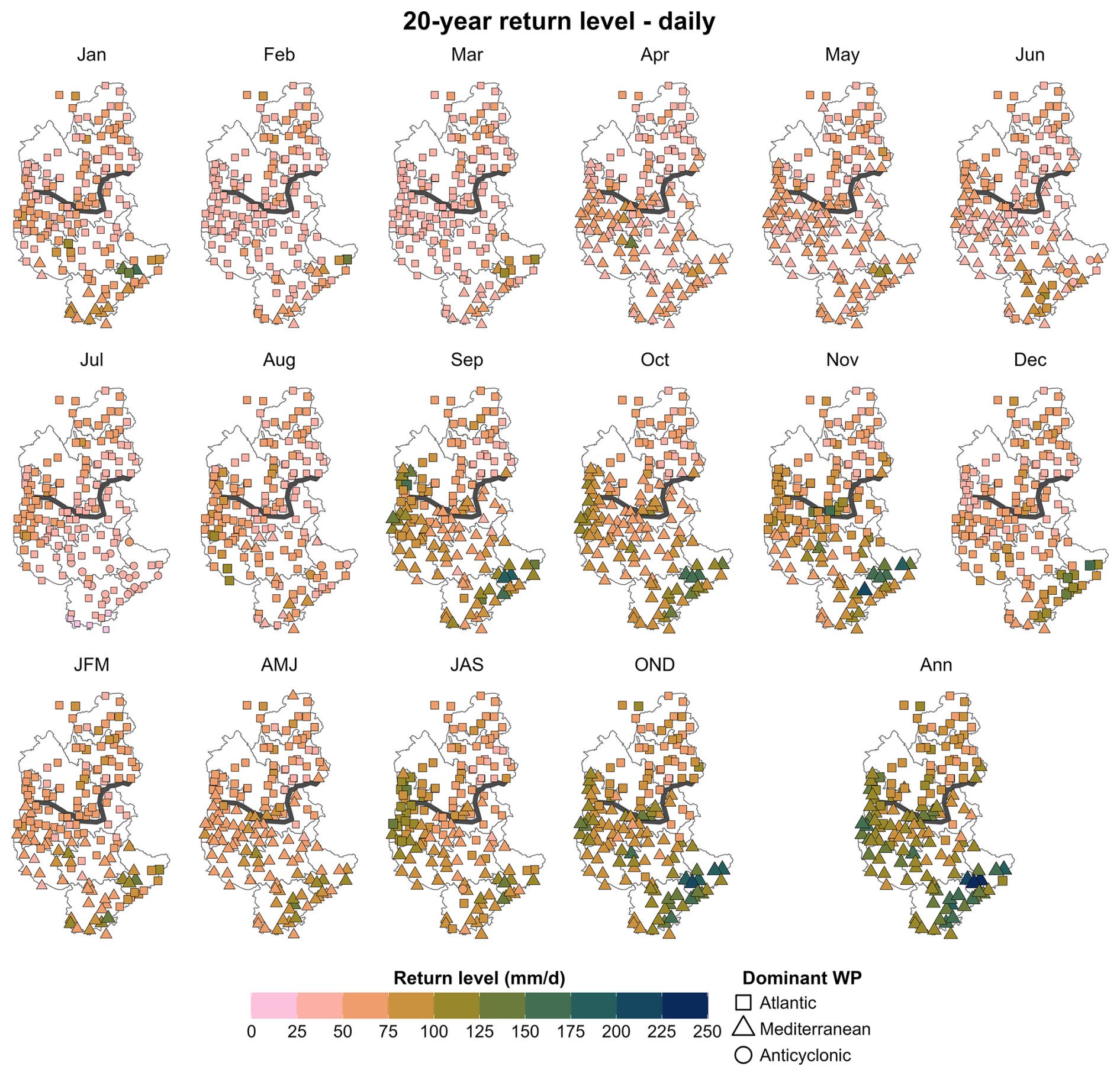
Figure 4 20-year return levels of daily precipitation extremes for EDF and Météo-France stations for the “recent” period (1980–2023). The colourscale and the size of the dots correspond to the amplitude of the 20-year return levels, the symbols to the dominant weather pattern. First and second row: monthly; third row: seasonal and annual.

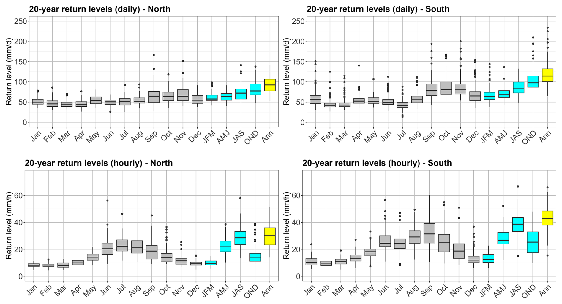
Figure 5 20-year return levels of daily (first row) and hourly (second row) precipitation extremes for EDF and Météo-France stations for the 'recent' period (1980–2023), grouped into stations north (left column) and south (right column) of the climatological divide.

4.1 Climatology of extremes

4.1.1 Daily precipitation extremes

Figures 4 and 5 show stationary 20-year return levels of daily extremes based on the “recent” observations (EDF and Météo-France, 27–42 years, earliest starting 1980). The return levels are lowest from February to August (< 70 mm d⁻¹) and higher between September and January (JAS and OND in the seasonal analysis), with the highest values from September to November. Daily 20-year return levels between September and January are also generally higher in the Rhône valley and along the Mediterranean coast. The highest values (> 200 mm d⁻¹) are found in the département of Alpes-Maritimes, in an area known for heavy autumnal precipitation. The lowest values of all regions and months (< 25 mm d⁻¹) in July in the southernmost areas reflect very dry conditions with almost no precipitation in this region during the summer months. The annual return levels very closely resemble those of the autumn season (OND).

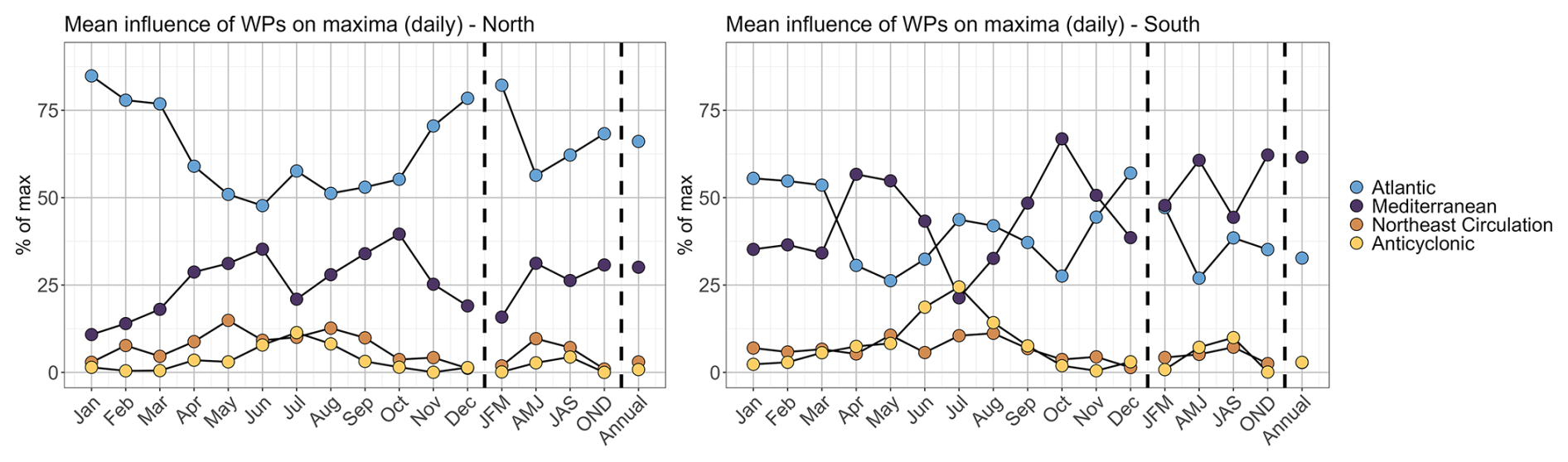
Figure 6 Relative influence of the four weather patterns on monthly/seasonal/annual maxima of daily precipitation intensity in the study region, for the period 1980–2023 grouped by stations north (left) and south (right) of the climatological divide.

In Fig. 6 we show the relative influences of the different weather patterns for monthly and seasonal maxima, averaged over all stations north and south of the climatological divide, respectively. In Fig. 4 just the most important (termed dominant) weather pattern is shown for each station. In general we find again the climatological divide between northern and southern Alps: In the north, the Atlantic influence dominates during the whole year. In the south, the influence of the Atlantic and Mediterranean flow oscillate in opposition of phase, the Mediterranean flow having the upper hand between April and June and September to November. When analysed seasonally, the Mediterranean flow remains dominant throughout the year. Some anticyclonic influence appears as important in the summer months (dominant only at some stations in the south). The annual patterns again resemble a lot the autumn patterns, showing the dominance of this season for annual precipitation maxima.

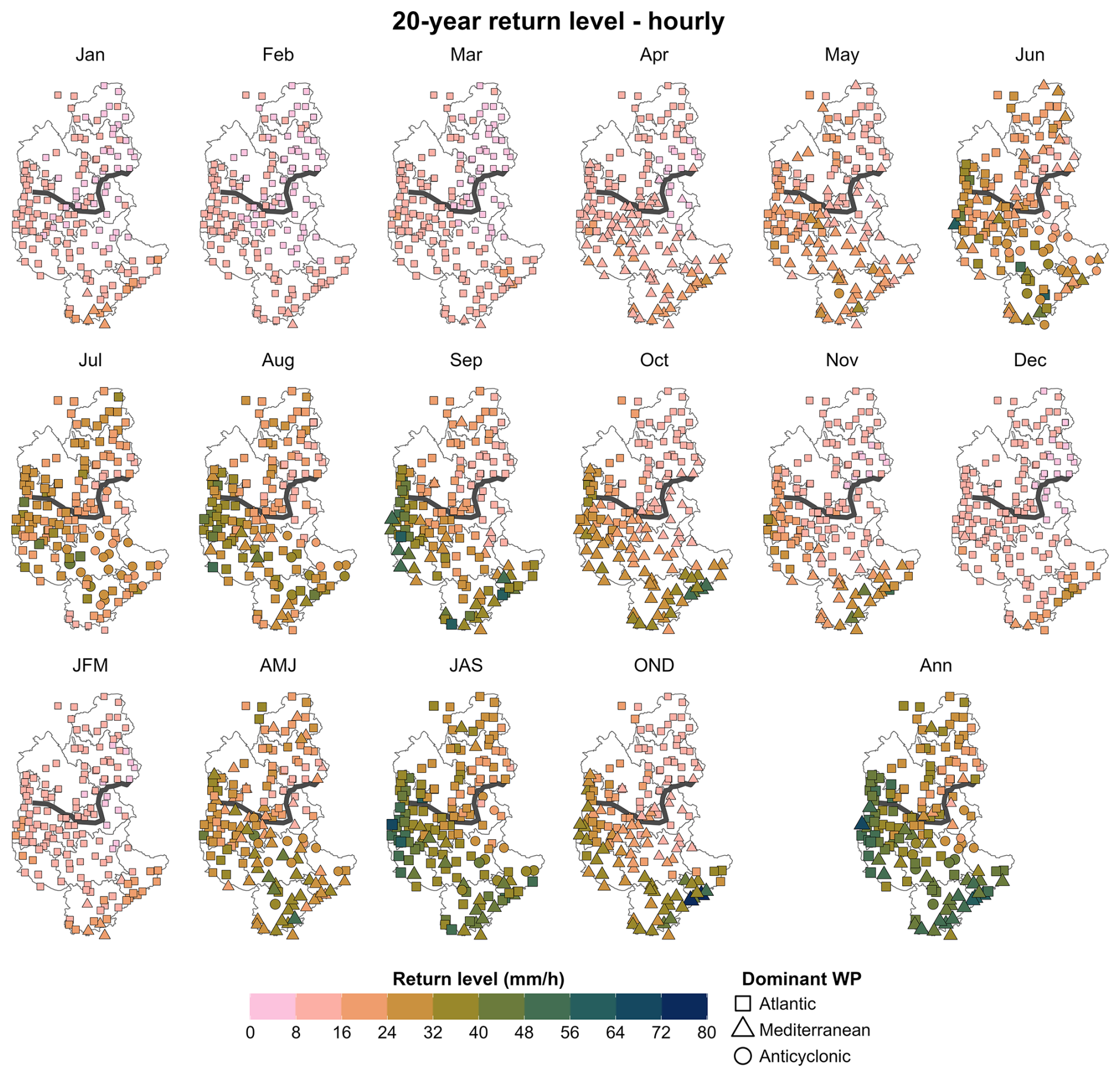
Figure 7 20-year return levels of hourly precipitation extremes for EDF and Météo-France stations for the “recent” period (1980–2023). The colourscale and the size of the dots correspond to the amplitude of the 20-year return levels, the symbols to the dominant weather pattern. First and second row: monthly; third row: seasonal and annual.

4.1.2 Hourly precipitation extremes

The stationary 20-year return levels of hourly precipitation reveal a seasonal cycle remarkably different from daily precipitation and across the north-south climatological divide (Figs. 5 and 7). The 20-year return levels are lowest in February (< 15 mm h⁻¹) and highest in late summer (August and September). In summer (JAS), the 20-year return levels show a distinct gradient between higher intensities in the pre-Alps and lower ones in the high inner Alps (centre-east of the study area). The highest 20-year return levels of all seasons can be found in September on the Mediterranean coast and in the Rhône Valley, and in July in western Alpes-de-Haute-Provence (04, Fig. 1) where estimates reach 75 mm h⁻¹ in some areas. Annual hourly extremes are dominated by the autumn season (OND) in the Rhône valley and along the coast, and by the summer season (JAS) in the inner Alps.

For the stationary analysis we only use “recent” data of stations managed by EDF (1980–2022) and Météo-France (1980–2023). For comparison, we also did the analysis using only EDF stations, but with all available data (i.e., the dataset used for the trend analysis). This did not result in very different spatial patterns (not shown). It should, however, be noted that almost no EDF stations are located in the parts of the study area with highest 20-year return levels (Rhône valley and along the coast).

Since hourly heavy rainfall depends on both the large-scale atmospheric circulation patterns and on local atmospheric conditions which drive convective processes, the analysis of the weather patterns by Garavaglia et al. (2010) is less robust for hourly than for daily maxima. The main patterns resemble the daily patterns, but with a higher influence of Anticyclonic conditions between May and August in the south of the study region (Fig. 7, see also Fig. S2).

4.2 Trends in extremes

We now turn to the trends in extremes (20 year return levels) over the period 1985–2022. Here we use only the long EDF time series covering 1952–2022 which, as noted above, include almost no stations in the Rhône valley or along the coast where stationary return levels are highest. Note that this entails that the region covered in Fig. 9 are not exactly the same as the region covered by the stationary return levels shown in Fig. 5. For easier interpretation we include the non-stationary 20-year return level estimates for the years 1990 and 2020 in the appendix, Figs. S3 and S4. We show the results in two different ways: (i) as boxplots of trends for each month and season, where stations are grouped by their location north or south of the climatological divide and (ii) on maps, where trends are shown for each station individually. Note again that the trends for each station are computed using a neighbourhood approach (see Sect. 3.2.2).

4.2.1 Trends in daily precipitation extremes

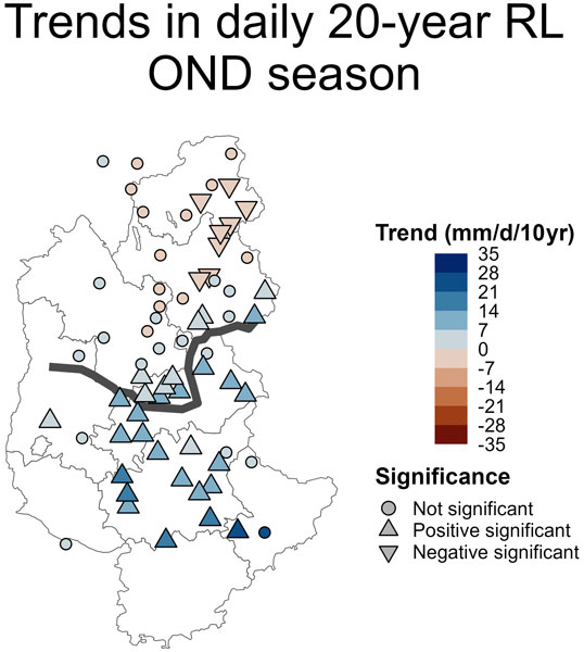
We find trends in daily extreme precipitation intensities mostly between −10 and +10 mm d⁻¹/10 years (Figs. 8 and 9). They show high variability between individual months/seasons but spatially coherent patterns. In the north of the domain, notable features include mostly significant positive trends in May, and significant negative trends in June and September. In the south of the domain, significant negative trends in August and September are followed by significant positive trends in October to December. Seasonal trends are overall negative in winter and summer (JFM and JAS) and positive in spring and autumn (AMJ and OND) seasons, while the trends at annual scale show a transition from significant positive trends (up to 24 mm d⁻¹/10 years or +50 % in 2020 relative to 1990) in the south to negative trends in the north (up to −8 mm d⁻¹/10 years or −20 % in 2020 relative to 1990), a pattern similar to the one found in autumn (OND, Fig. 9, upper row).

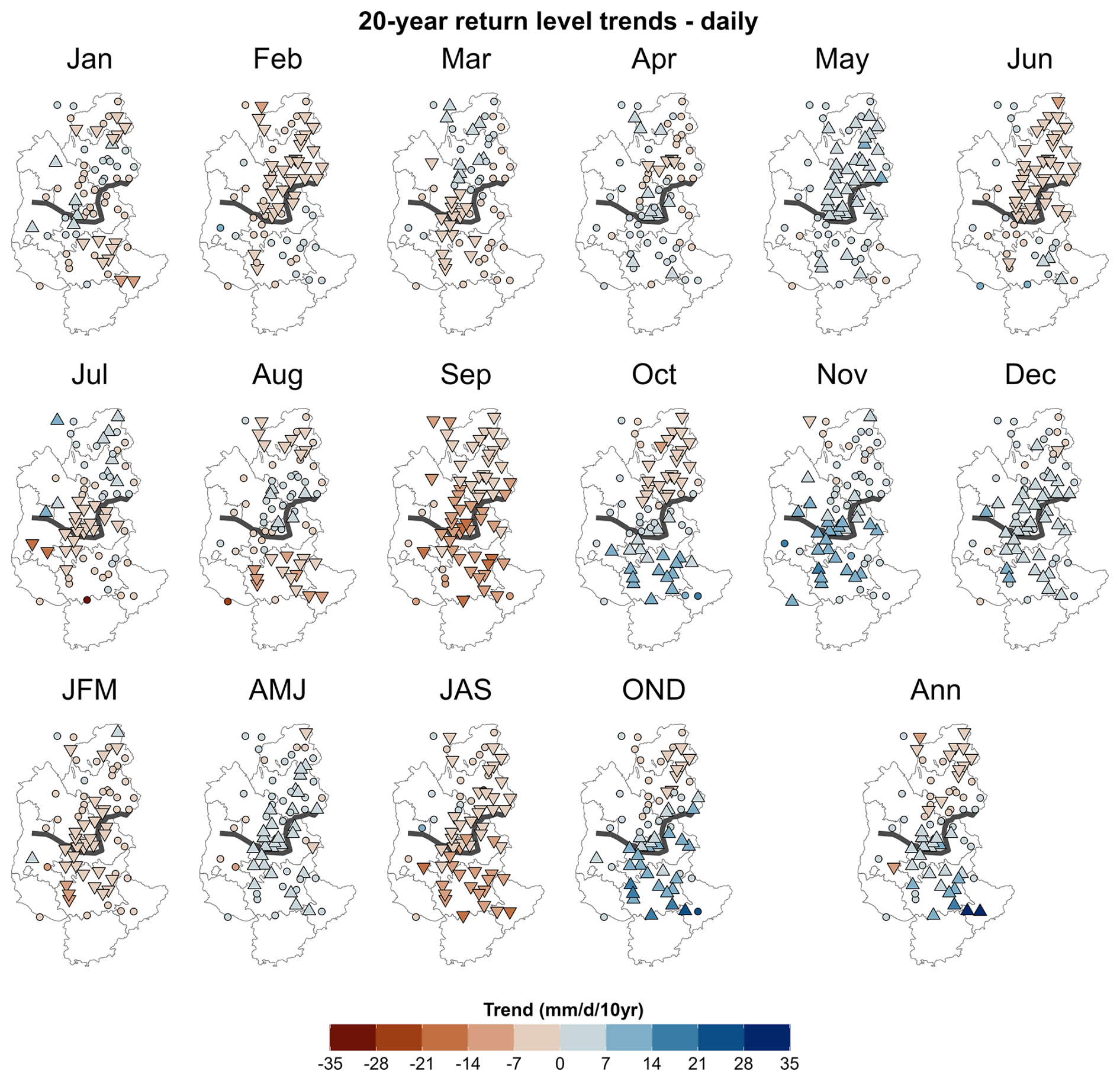
Figure 8 Trends of 20-year return levels of daily precipitation intensity between 1985 and 2022 using the nonstationary framework with a neighbourhood approach. Upward triangles indicate significant positive, downward triangles significant negative trends, and round points non-significant trends (positive and negative). First and second row: monthly; third row: seasonal and annual.

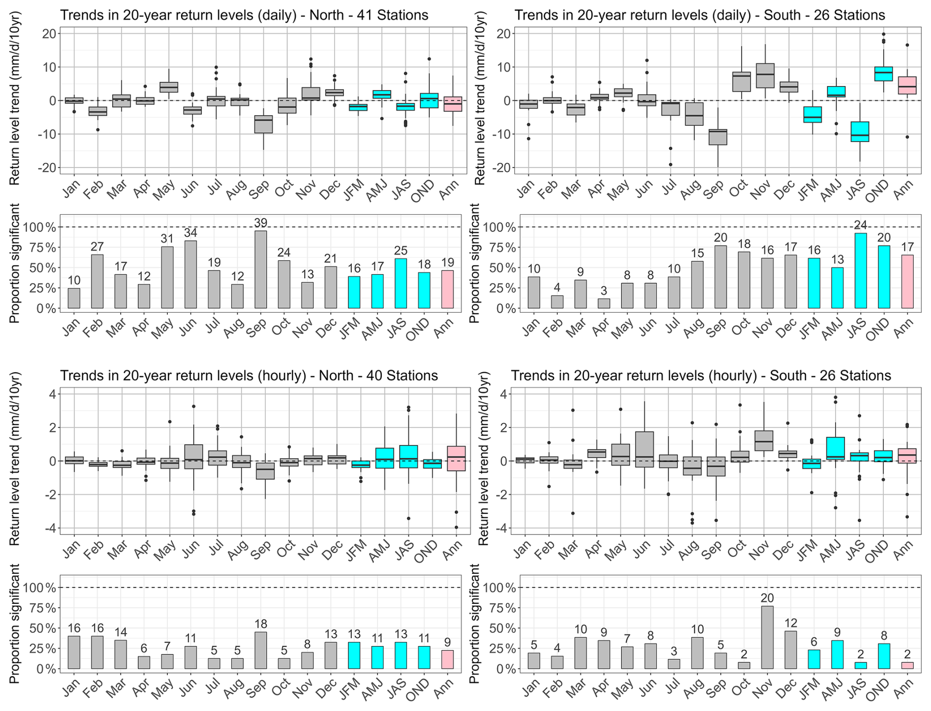
Figure 9 Trends of 20-year return levels of daily precipitation intensity between 1985 and 2022 using the nonstationary framework with a neighbourhood approach for daily (first row) and hourly (third row) precipitation extremes using all available time series of EDF stations (including “old” data) covering at least 34 years between 1952 and 2022 (66 of both hourly and daily data, 1 of daily data only). Both statistically significant and non-significant trends are included. The relative share and absolute number of stations with significant trends are shown in the second (daily) and fourth (hourly) row. The results are grouped into stations north (left column) and south (right column) of the climatological divide. For visualisation purposes the y-axis has been limited at ±20 mm d⁻¹/10 years for daily and at ±4 mm h⁻¹/10 years for hourly data, removing in total four daily and 16 hourly data points.

4.2.2 Trends in hourly precipitation extremes

Trends in hourly precipitation extremes (shown in Figs. 9 and 10) are highly variable both spatially and between individual months/seasons. Overall, the trend is significant at much fewer stations than for daily precipitation, and the number and location of such stations varies considerably from month to month and season to season. In the north of the domain, trends are almost always centred around zero (September with comparatively small negative trends being an exception), with the widest range of values (and highest absolute values) in June and very small ranges during December to April (Fig. 9, l.l.). In the south, variability around the mean is higher for most months. Overall positive trends can be found in April to June and October to December, while they tend to be slightly negative in August and September (Figs. 9, l.r. and 10). November stands out as the only month where a spatially coherent pattern appears showing significant positive trends in the south (up to +3.5 mm h⁻¹/10 years or +100 % in 2020 relative to 1990, Fig. 10). Looking at seasons, trends in the north are also overall centred around zero, with the largest variability and some areas with significant positive trends in spring and summer (AMJ and JAS, Fig. 9, l.l.). While the picture in the south looks similar overall, spring (AMJ) stand out with overall positive trends and highest variability (Fig. 9, l.r.). Annually, trends are centred around zero with comparatively large variability in the north and overall slightly positive in the south, although the annual trends in the south are statistically significant at only 2 of the stations, and are of opposite sign. While we here decided to only look at the climatic north-south division of the study area, it should be noted that looking at JAS and annual extremes in Fig. 10 there seems to be a northeast-southwest pattern, with positive trends in the northeast (high Alps) and negative ones in the southwest (lower Alps),

Despite the lack of clear patterns in the trends of hourly extremes there are some systematic differences to the trends in daily extremes: in summer (JAS), trends in daily extremes are overall negative, while they are mostly close to zero or positive for hourly extremes. Also, the clear north-south pattern in trends found for daily extremes in autumn (OND) is completely absent in the hourly data, where weakly non-significant and weakly negative trends prevail over the whole region.

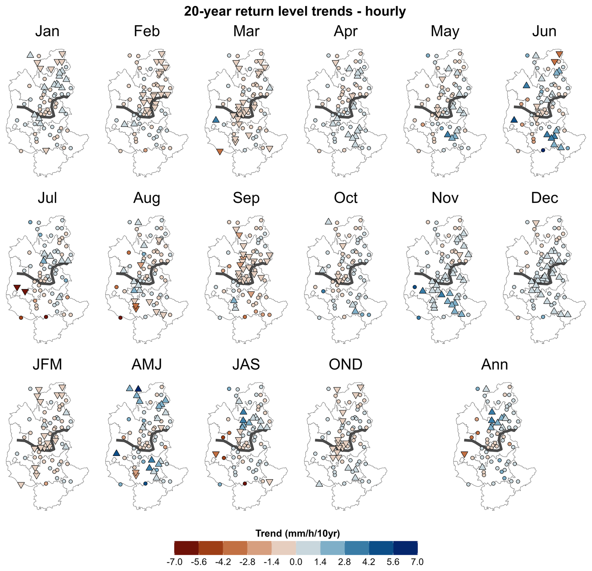
Figure 10 Trends of 20-year return levels of hourly precipitation intensity between 1985 and 2022 using the nonstationary framework with a neighbourhood approach. Upward triangles indicate significant positive, downward triangles significant negative trends, and round points non-significant trends (positive and negative). First and second row: monthly; third row: seasonal and annual.

5 Discussion

5.1 Methodological limitations

5.1.1 Sampling bias

In this study we applied extreme value theory on time series data spanning at least 25 years of observations. While this method is widely used in the study of extremes, it also has its limitations. The return level estimates heavily depend on the quality, length, and variability of the time series. In some cases the presence (or absence) of single events can significantly influence return level estimates (Zeder and Fischer, 2024). For example, in Figs. 4 and 7, some individual points stand out from their surroundings, which is probably due to a sampling bias and not due to a strongly different climate of this station to its surroundings. However, as mentioned earlier, the general patterns for stationary return levels are largely consistent and seem plausible given previous studies (e.g. Djerboua, 2001), which gives us confidence in the methodology and in the interpretation of trends. To a certain extent, more robust return level estimations can be obtained by using a neighbourhood or region-of-influence approach, reducing the sampling bias by using more data, as we do here for the non-stationary trend estimations.

5.1.2 Nonstationarity and regional approach

We applied a non-stationary framework to take trends in return levels into account and thus better assess the changing hazard in the context of global warming. However, a drawback is that non-stationarity requires more parameters to be estimated, which adds additional uncertainties: (i) We assume that the parameter distribution changes linearly with time. In many regards this is a simplification, as there is no direct physical dependence of precipitation parameters on time. Indeed, in light of previous studies analysing the temperature – precipitation relationship (e.g. Da Silva and Haerter, 2025), temperature might seem like an obvious choice. However, which temperature to choose (e.g. local temperature at the time of the event, dew point temperature at a given pressure level, annual region-mean temperature, or sea surface temperature) is a debate of its own (see also Schröer and Kirchengast, 2018; Dash and Maity, 2023; Zeder and Fischer, 2020; Haruna et al., 2026), which is why we chose to keep time as the simplest covariate. In general, the temperature evolution at reference stations by Météo-France in the region seems to have been roughly linear since the mid 1980s (see https://meteofrance.com/climathd, last access: 19 October 2026, based on data by Gibelin et al., 2014), which leads us to argue that assuming a linear evolution of extreme precipitation intensity with time since 1985 is justified. (ii) From a statistical perspective, introducing time as a covariate means additional parameters to estimate, which in turn results in higher uncertainty in the estimates if the same amount of data is used. Here, we use a neighbourhood approach to overcome this problem: we combine the observed maxima at each individual station with the scaled maxima of its surroundings, thus significantly increasing the number of data points available for return level estimation. However, this approach comes with another strong assumption: We assume that the neighbourhood of each station is statistically homogeneous, which is not necessarily the case. Other studies (e.g. Carreau et al., 2013; Evin et al., 2016) have used an iterative procedure combined with a homogeneity test to find the best radius for each station. In our experience homogeneity tests such as the Hosking and Wallis (Hosking and Wallis, 1997) test tend to be too permissive, i.e. they tend to falsely classify nonhomogeneous region as homogeneous, thus resulting in too large neighbourhoods (for a simulation study see Evin et al., 2016), which is why we decided against using this method in our study. With the radius of 0.3° we are using here we find trends that appear spatially coherent. We also tried different radii of 0.2 and 0.4° and found that the general picture remains quite similar. Thus, as long as we are mainly interested in the broader picture instead of particular values, the choice of the radius actually seems secondary to us.

It is interesting to note that, even though the neighbourhood approach helps getting robust and spatially coherent results for daily extremes (e.g. Fig. 8), our results for hourly extremes appear noisier (Fig. 10). This is probably due to the combination of relatively short time series of a few decades, the high interannual variability, and the very localised character of extreme short-duration precipitation events (see also Barbero et al., 2017). Given that EDF's station network is already comparatively dense with quite long observations we here arrive at the current limits of studying precipitation extremes based on surface observations. However, future studies with longer time series (and the additional observations from Météo-France’s network starting in the 1990s soon to become long enough to be included) have the potential to result in more robust and spatially coherent trend estimations.

5.1.3 Estimation of seasonal and annual return levels

Estimating a single distribution over a time series assumes that all data come from the same distribution. This is challenging in the real world because, for example, extreme precipitation maxima can be generated by very different meteorological mechanisms, such as stratiform or convective precipitation (see also Da Silva and Haerter, 2025, for the consequences of this) and different circulation patterns (Blanchet et al., 2021a, b). By using a monthly analysis, we can overcome this problem to some extent, as precipitation extremes are likely to be caused by a dominant weather type in individual months. We can extend this assumption to the different seasons, as in general, a weather pattern dominates in each season (Figs. 6 and S2), with however the exception of hourly seasonal maxima in the south (Fig. S2). The same applies to annual maxima. Including the fact that daily annual maxima almost exclusively stem from OND and hourly annual maxima from JAS (see similarities in Figs. 6 and S2) we conclude that the homogeneity assumption is reasonable for both monthly, seasonal, and annual maxima.

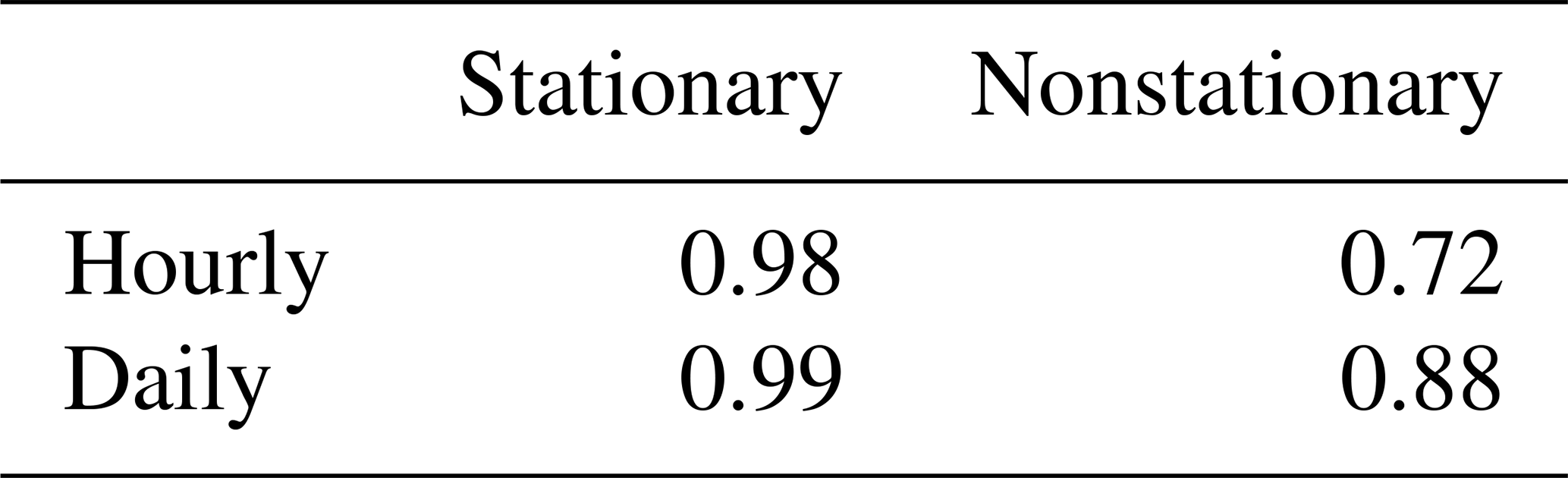
As already mentioned in Sect. 3.1, an alternative approach for estimating return levels would be to analytically derive the seasonal and annual distributions directly from the monthly distributions (by multiplying them). However the drawback of this is that, if some monthly fits fail for any reason, the errors will propagate through seasons and year. We compared both methods – fitting the GEV to the corresponding maxima (as in this article) versus analytically deriving the seasonal and annual distributions from the monthly maxima – and find that in the stationary analysis, deriving the distributions from the monthly maxima gives erroneous results in return levels compared to the empirical estimates (Fig. S5). The reason why some monthly fits fail is unknown but could be due to measurement errors, or sampling bias, as discussed previously. A possible compromise would be to fit the seasonal distributions on seasonal maxima (as we have done here) and only derive the annual distribution from these. In this case, we find comparable results between the two methods (Table 1, Figs. S6 and S7). Unfortunately, due to the limited amount of data, it is not possible to compare the trend estimates to an empirical analysis in the nonstationary case, and therefore we cannot know which method performs better. This said, we have compared the trend in the 2-year return level (which corresponds to the median of the data) to the trend in the median, and find comparable results for both methods (not shown). Similar results have been shown by Maraun et al. (2009), leading them to conclude that annual maxima provide overall reasonable return level estimates. Considering annual maxima for estimating GEV distributions is anyway very common (e.g. Papalexiou and Koutsoyiannis, 2013; Ben Alaya et al., 2020; Ribes et al., 2019; Jayaweera et al., 2023).

An option to make monthly fits more robust is to fit a GEV on all months, linking them by prescribing that the GEV parameters of the individual months have a seasonality (μ=μ_month), which would have the advantage of a stronger constraint on the monthly fits (Maraun et al., 2009; Fischer et al., 2018; Raillard et al., 2026). The annual return levels could then again be derived from these monthly fits. For daily, stationary analysis, Maraun et al. (2009) have shown that the two approaches (linking the GEV parameters or estimating them independently) are comparable. For nonstationary analysis, we are only aware of one study that included long-term trends in such a model (Raillard et al., 2026), which, however, analysed sea-state variables in CMIP6 models. In our study we analyse a much smaller dataset and a variable that is more prone to outliers, either due to singular extreme events or measurement errors. Furthermore, we do not find a reasonably smooth seasonality in the estimated monthly GEV parameters, which is why we did not pursue this approach.

Table 1 Correlation between two different methods for estimating annual 20-year return levels (stationary) and trends in these return levels (nonstationary). Method 1: estimate based on annual maxima; method 2: estimate based on seasonal CDFs.

5.2 Climatology of extreme precipitation

We now turn to a discussion of the climatology of stationary return levels. Daily precipitation intensities (Fig. 4) remain quite constant over the whole year in the north (most notably in Savoie and Haute-Savoie), which is also in line with the large dominance of Atlantic influence on precipitation maxima in this region (Blanchet et al., 2021a, b, see also Fig. 4 in our study). In the south and along the Rhône valley the months from September to December stand out with much higher 20-year return levels than the rest of the year, which is characteristic of the precipitation seasonality in the Mediterranean area. Here, very dry summers are followed by rainy autumn and winter seasons, an effect enhanced by orographic uplifting of moist air masses originating from the Mediterranean Sea along the southern and southwestern slopes of the Alps.

20-year return levels of hourly precipitation intensities (Figs. 7, 5) follow a clear annual cycle with low values during winter (JFM) and high values during late spring (June) and summer (JAS). This can be explained by the higher humidity and convective available energy during the warm season, which can trigger intense but localised convective events like thunderstorms. Interestingly, when comparing south to north, the peak of this cycle is higher and occurs later in the year in the south (Fig. 5), which suggests an influence of the Mediterranean flows also on the annual cycle of hourly return levels. This strong cycle shows the added value of analysing extreme precipitation at monthly resolution as we do here. A seasonal analysis would miss this monthly non-stationarity, for example the aspect that hourly precipitation extremes in spring (AMJ) are largely dominated by the month of June and thus not representative of the whole season.

Two more aspects of the geographical distributions are worth highlighting here: First, the very low return levels found at some stations along the coast in July, again showing the arid conditions typical for the Mediterranean region. Second, the spatial distribution of hourly extremes, showing higher return levels along the southern and western slopes and pre-Alps compared to the inner Alps, a pattern consistent with the findings of Fukutome et al. (2015); Panziera et al. (2018) for Switzerland. Panziera et al. (2018) attribute this to the role of the first Alpine slopes triggering convection in unstable airmasses arriving from the west or south, and Fukutome et al. (2015) note that there is a lack of sufficient moisture convergence in the inner-Alpine zones.

5.3 Trends in extremes

In the following section we discuss the trends found for hourly and daily 20-year return levels in the French Alps. A special emphasis is put on the differences between trends for hourly and daily extremes, which we consider at least as informative as the actual trends themselves.

First, we find clear differences between the north and the south of the region also for the trends in daily extreme precipitation (Fig. 9), which is in line with previous studies (Blanchet et al., 2021a, b). Between June and December, the southern part of the study region experiences much stronger trends, both positive and negative, for both hourly and daily extremes. Note that for hourly extremes, trends are never statistically significant at more than half of the stations, with the exception of November. In the south, daily trends tend to be negative when the Mediterranean influence is weak (January to March, July to September) and positive where it is stronger. This is a strong indication of the importance of weather patterns not only in generating extremes, but also in explaining trends in their intensity.

Still looking at the south, especially the autumn period (OND) deserves attention, as in this period both strong, mostly significant positive trends in daily extremes, a strong influence of Mediterranean flow patterns (our study) and also a strengthening of this influence (Blanchet et al., 2021b) are observed. We thus speculate that the positive trends can partly be attributed to an increase in Mediterranean sea surface temperature in summer and autumn (Pastor et al., 2020), causing higher humidity in the atmosphere which is then advected to the southern French Alps by southerly/south-westerly fluxes.

While hourly extremes also show positive trends during the same months as daily extremes (Fig. 9), the clear negative trends in summer (JAS) shown for daily extremes are much weaker or absent in the hourly values. Indeed, in the south between June and September, there is a very clear difference: hourly trends are overall small, often not significant, and spatially variable but also include comparatively high positive trends locally, especially in June. Daily trends in the same period and region are overall negative. To a lesser extent this is also true in June in the north, showing that during this time of the year hourly and daily extremes are not experiencing the same trends.

These observed differences, together with the analysis of dominant influences shown in Sect. 4.1 give us some ideas on the reasons of the trends. The strong negative trends of daily precipitation in summer (JAS) are likely to be a direct consequence of generally less precipitation in this region (e.g. Menegoz et al., 2020), which is already characterised by low precipitation totals (Joly et al., 2010). Trends of hourly extremes in the same season show both negative and positive trends, with significant positive trends especially at several stations in the northeastern part of the region, where the mountains are highest. While this is clearly different to the daily trends, negative trends or trends close to zero are also not in line with the increase which could be expected by the Clausius-Clapeyron relationship, given that we observe a temperature increase in the region (Gibelin et al., 2014). These trends might be the result of a tug-of-war between less moisture available for local recycling due to increasing aridity (Tramblay et al., 2020) and increasing energy availability due to increasing temperature. Unfortunately we do not have temperature measurements at EDF rain gauge stations and thus cannot do a direct comparison with measured temperature, however, based on a regional climate model forced by ERA-20C reanalysis Beaumet et al. (2021, their Fig. 5) show that temperature trends over 1959–2010 are highest in summer (JJA) in the interior regions of the French Northern Alps, which roughly coincides with the region of significantly positive hourly trends in our results (Fig. 10, Annual). We further hypothesize that the drying effect might dominate in the pre-Alps (small to negative trends in some southwestern parts of the region), while the increase of available energy might dominate in the interior of the Alps leading to positive trends in the northeastern part (Fig. 10). This would also match the findings of e.g. Giorgi et al. (2016) who used an ensemble of regional climate models to show increases in convective precipitation in summer in the high massifs of the European Alps. This could be attributed to albedo feedback loops, where decreasing snow cover leads to additional surface warming, an effect that has been shown for intermediate altitudes (1500–2000 m a.s.l.) in our study region (Beaumet et al., 2021). This in turn increases thermodynamic instabilities and the potential for convective precipitation. In this regard, it would be interesting to also study trends on subhourly timescales. However, stations maintained by EDF unfortunately do not register at such small timesteps, and observations registered by Météo-France at 6-minute intervals are still too short for a robust analysis of trends. At this point it should be noted that a comparatively dense network of observations by Météo-France exists in the Drôme region (départment no. 26, Fig. 1) with continuous observations at subhourly (six minutes) resolution starting in 2005. We decided to not include this dataset here due to the short period and the limited area covered. Another potential source of information with high spatial resolution could be radar observations. However, they also cover just a limited period of time and come with different limitations, such as masking in mountainous regions and inhomogeneities in time.

The month of September where a significant and strong decrease in daily extremes is observed over the whole study region deserves special attention: most likely, this result can be attributed to a shift in seasonality with a later onset of the rainier autumn season. This means that September would be shifting from being an autumn month (which is still visible in the stationary return level estimations) to being a summer month (see also Fig. S3), an observation shared by stakeholders in the region (pers. comm. from stakeholders at RTM, EDF, Météo-France). A later timing of autumnal period of high precipitation intensities might also explain the significant increase in intensity of both daily and hourly precipitation extremes in November which appears small in absolute numbers (+8–16 mm d⁻¹/10 years for daily precipitation extremes or +1–4 mm h⁻¹/10 years for hourly precipitation extremes, Fig. 9) but is large in relative terms with increases up to +60 % (daily) and +100 % (hourly) between 1990 and 2020 (not shown). A similar shift could also explain the significant trends with opposite sign of daily extremes in May and June in the north, with increasing trends in May and decreasing trends in June. This “new” timing of seasons poses significant challenges for defining seasons for trend assessment. A potential way to solve this problem might be to define the seasons dynamically, for example by using threshold values for precipitation characteristics for each season. However, this was out of the scope of our study.

6 Conclusions

In our study, we present an updated climatology and trend analysis of precipitation extremes across the French Alps, applying a statistical approach based on extreme value theory (Coles, 2001; Fisher and Tippett, 1928) on long time series of hourly and daily surface observations. We find distinct spatial patterns with marked differences between daily and hourly timescales. Most notably, we show that precipitation extremes do not generally scale with temperature as could be expected by the Clausius-Clapeyron relationship, which also implies that estimating future changes of precipitation extremes in the region would be a difficult task.

For daily precipitation extremes, we find robust positive trends in the southern French Alps, particularly during autumn (OND), driven by an enhanced influence of southerly (Mediterranean) flow patterns. Conversely, the northern French Alps show negative trends, possibly due to changes in Atlantic flow patterns. At the hourly timescale, trends are more spatially variable, with a tendency towards positive trends prevalent in the high mountain ranges in the northeastern parts of the study domain. We hypothesise that this pattern might be a result of counteracting changes in the availability of moisture and energy for convective precipitation. The seasonal and spatial differences underscore the complex interplay between large-scale circulation patterns, thermodynamic effects and regional topography. This also provides a rationale for analysing extremes at monthly or seasonal scales as well, as by looking solely at the annual scale one would miss some important trend signals.

While the observational dataset we analyse here is already comparatively dense and contains long time series, future research making use of data with even higher spatial and/or temporal resolution (e.g. radar observations) could help to get further insights into the dynamic and thermodynamic processes at play. More research is also needed to further analyse the influence of changes in seasonality and flow patterns. For example, one hypothesis for the decrease in daily extremes in the north of the study area could potentially be a change in the angle between the atmospheric flows bringing moisture relative to the orientation of the main mountain chains, which could be a consequence of global climate change or a signal linked to natural climatic variability.

We find the strongest increases in the regions and seasons which are already at the highest risk of strong-impact events, i.e. in autumn (OND) in the south for daily precipitation extremes and in June as well as November for hourly extremes. This is reflected in the annual trends, showing increases in the south of up to 24 mm d⁻¹/10 years for daily, and increases in the inner Alps of up to 4 mm h⁻¹/10 years for hourly extremes, confirming local stakeholders' perception of changes (personal communication from stakeholders at RTM, EDF, Météo-France). Overall, the French Alps with their diverse climatic influences and topographic complexity provide an ideal example of the importance of region-specific and timescale-specific analyses for estimating current and future trends in precipitation extremes and its associated risks, such as flash floods and land slides.