The need for uncertainty: why probabilistic LSTMs are key to improving flood predictions and enabling learned warning rules

Deterministic model predictions can struggle to adequately capture extreme events such as floods and droughts, which are of particular importance in hydrology. This limitation arises because deterministic models collapse the conditional discharge distribution to a single point estimate. Probabilistic modeling provides a way to address this issue by explicitly representing uncertainty and assigning non-zero probabilities to all possible outcomes, including extreme events, thereby capturing the entire conditional discharge distribution. Motivated by this perspective, we examine whether probabilistic Long Short-Term Memory (LSTM) models improve the representation of extreme events in rainfall–runoff simulations across Switzerland. The differing degree of flexibility in the models leads to different degrees and distinct patterns of miscalibration in the predictive distributions. For the extreme discharges (top 0.05 % of the marginal discharge distribution), the deterministic LSTM systematically underestimates 97 % of these events, whereas 83 % of these fall within the probabilistic model's 99th percentile prediction interval. Given the rarity of these events, representing them as outcomes near the upper tail of the predictive distribution is both expected and statistically consistent. Building on the additional information provided by probabilistic runoff predictions, we further show how they can be translated into actionable flood warnings using reinforcement learning. To this end, we introduce a Flood Risk Communication Agent (FRiCA) that operates on probabilistic runoff predictions and learns risk-aware decision rules for issuing warnings of varying intensity. Results indicate that the FRiCA outperforms simple fixed heuristics, such as issuing warnings based on the deterministic LSTM predictions or a fixed high quantile (e.g., the 99th percentile). The learnt behavior demonstrates the potential of reinforcement learning as a decision layer for improved flood risk communication, and motivates further exploration of better reward design and policy network optimization for context-dependent decision policies that adapt to varying hydrological and societal contexts.

1 Introduction

Deep learning (DL) models, particularly Long Short-Term Memory networks (LSTMs; Hochreiter and Schmidhuber, 1997), have established themselves as a powerful alternative to traditional hydrological modelling approaches and are now the benchmark for rainfall–runoff modeling across varying hydrological settings (Kratzert et al., 2019a). Ever since, much research has focused on applying LSTMs in different regions of the world (Lees et al., 2021; Loritz et al., 2024; Frank et al., 2023; Clark et al., 2024) and on further improving its predictive performance. However, as their application becomes increasingly widespread, a growing body of research is now examining the conditions under which LSTMs reach their limits (Baste et al., 2025; Heudorfer et al., 2025). In particular, an important open question concerns their ability to reliably predict hydrological extremes. When evaluated globally, as an aggregation over long hydrological time series, LSTMs outperform conceptual and process-based models (Kratzert et al., 2019a; Lees et al., 2021). However, their advantage can weaken substantially when confronted with rare, high-magnitude events. Frame et al. (2022) employed a stress-testing approach in which models were trained on an intentionally truncated dataset, excluding all years containing floods exceeding a 5-year recurrence interval. They found that with increasing event magnitude (higher recurrence period), the bias in LSTM predictions increases. Using a similar experimental setup, Acuna Espinoza et al. (2025) compared an LSTM with hybrid model variant (from Feng et al., 2022) and a conceptual model (the Hydrologiska Byråns Vattenbalansavdelning (HBV) model; Bergström, 1992). Once again, their results showed that the performance advantage of the LSTM decreases as flood magnitude increases, with all three models showing similar underestimation for the events with the largest recurrence period. These findings suggest that the strong performance of LSTMs relative to traditional models does not automatically extend to the tail of the marginal discharge distribution. This poses a significant limitation given the importance of extremes in hydrological forecasting, risk assessment, and operational decision-making.

To further investigate the behavior of LSTMs when predicting extremes, we analyzed their extrapolation performance in Swiss catchments (Baste et al., 2025) and found that, although the training data contained peak flows of up to ∼180 mm d⁻¹, the LSTM failed to produce discharge beyond a theoretical ceiling of ∼120 mm d⁻¹. Building on this finding, we designed a new stress-test approach wherein the most extreme precipitation events in the test period were replaced by design storms with annual return intervals of 50, 100, and 300 years. Such an approach simulates current infrastructure design practices and is directly relevant for the evaluation of high-impact floods. These stress tests showed that the LSTM not only underestimates the flood response for these unseen extremes, but also exhibits an empirical upper bound of ∼75 mm d⁻¹, which is significantly lower than the theoretical prediction limit. These findings are consistent with the gating-related limitations discussed in Kratzert et al. (2024). This systematic underestimation persists across the tail of the marginal discharge distribution, even when flood-peak magnitudes expected for the design storms are present in the training data. Together with the results of Frame et al. (2022) and Acuna Espinoza et al. (2025), these findings provide converging evidence that LSTM architectures, and the way in which they are currently applied, exhibit constraints when used for extreme events prediction, and more so in situations that require extrapolating beyond historically observed precipitation magnitudes. However, this does not represent a dead end; several promising modelling strategies offer potential pathways to overcome these limitations. Baste et al. (2025) explored some strategies to improve the extrapolation of LSTMs, including increasing the amount of training data following Kratzert et al. (2024), adapting the loss function, and modifying the activation functions within the LSTM. While these adjustments resulted in small improvements, none of them resolved the core issue, and the LSTMs continued to exhibit restricted simulations for the highest floods and a persistent bias for extreme values. Notably, strategies that improved the representation of the extreme events did not guarantee sustained global performance at par with the LSTM. Essentially, some of our endeavours left us with specialist models that represented extremes well, at the cost of the poor representation of other flow regimes.

This persistent underestimation bias – observed across architectures and mitigation strategies alike – points to a more fundamental cause rooted in the inherent uniqueness of hydrological response generation and how different models learn to represent it. In hydrological modelling, identical or similar sequences of meteorological forcing can produce multiple, non-identical hydrological responses. For example, a 50 mm d⁻¹ rainfall event may or may not trigger an extreme flood response, depending on antecedent soil moisture, snow conditions, seasonality, and the internal catchment state. Hydrological systems are, in principle, deterministic and their future evolution is uniquely defined by dynamical laws, given complete knowledge of all relevant states (Lorenz, 1963; Sivapalan et al., 2003). In other words, given complete knowledge of a catchment, it should theoretically be possible to uniquely determine the hydrological response from the forcing and the system state. In practice, however, this theoretical determinism breaks down. Hydrological models, especially those using large sample datasets, are subject to errors in meteorological and hydrological observations, their spatial aggregation at the catchment level, uncertainty in internal storage states, equifinality, and limitations in how models represent or retain these states (Beven and Freer, 2001; Montanari and Di Baldassarre, 2013). As a result, they struggle to map similar forcings onto the corresponding range of plausible hydrological responses. From a statistical learning perspective, a model is asked to infer a deterministic mapping for inherently uncertain input-target dynamics. Depending on the loss function, the learning process then elicits a specific functional of the conditional target distribution (Gneiting and Ranjan, 2011). A common loss function for LSTMs is the mean squared error (MSE), which elicits the mean of the conditional discharge distribution. By definition, the mean lies below the upper parts of a distribution. For discharge predictions, the difference in the mean and the upper quantiles is even more tangible, since the conditional distributions are typically right-skewed, with a long tail toward high-magnitude events. Consequently, for uncertain input-target relationships, this elicitation can lead to regression-to-the-mean behaviour and a systematic underestimation of extreme events. Modifying the deterministic loss functions still elicits only a single functional of the conditional distribution, whereas a probabilistic model predicts the full conditional distribution, of which the upper quantiles – rather than the mean – are directly relevant to flood risk. This highlights why probabilistic LSTMs are conceptually better suited for predicting extreme floods.

This theoretical case for probabilistic prediction is reinforced by long-standing applied literature: uncertainty quantification has been recognised as a central challenge in hydrology for decades (Krzysztofowicz, 2001; Beven and Freer, 2001). Cloke and Pappenberger (2009) reviewed the use of ensemble prediction systems (EPS) for flood forecasting and demonstrated the advantages of ensemble hydrological prediction across several European case studies. Bálint et al. (2006) reported that ensemble hydrological predictions improved the capability to issue flood warnings during the August 2002 floods at the Devin and Budapest gauging stations. Roulin (2007) investigated long-term hindcasts for two Belgian catchments and demonstrated that probabilistic forecasts outperformed deterministic ones, yielding greater economic value within a cost-loss decision framework. Several studies on EPS for hydrological forecasting likewise emphasize the added value of probabilistic information in providing a “clear indication of the possible occurrence of the event” (Roulin and Vannitsem, 2005) and “the indication of the possibility of an extreme event” (Gouweleeuw et al., 2005).

A first step in addressing uncertainty in hydrological deep learning was taken by Klotz et al. (2022), who introduced several methods for uncertainty estimation in a regional rainfall–runoff model trained on the CAMELS-US (Catchment Attributes and Meteorology for Large-sample Studies – US Addor et al., 2017) dataset. Their results showed that mixture density networks (MDNs), particularly the Countable Mixture of Asymmetric Laplace (CMAL) model, produced the most reliable predictive distributions. We investigate whether probabilistic predictions can help overcome the systematic underestimation of extreme floods observed in deterministic LSTMs. To this end, we compare three complementary probabilistic approaches that represent predictive uncertainty in different ways: the Countable Mixture of Asymmetric Laplace (CMAL) model (Klotz et al., 2022), a Distributional Regression Network (DRN) that predicts the parameters of a parametric distribution (Rasp and Lerch, 2018), and a Bernstein Quantile Network (BQN) that directly estimates the predictive quantile function (Bremnes, 2020). Together, these approaches span a range from strongly parameterized to highly flexible distributional representations, allowing us to assess whether improved characterization of predictive uncertainty translates into a better representation of extreme floods.

A major drawback of probabilistic forecasts is that operational flood management ultimately requires discrete decisions. While probabilistic models provide a full predictive distribution and can explicitly represent the possibility of rare but high-impact events, flood warnings must eventually be issued (or not issued) at a specific warning level. Consequently, the predictive distribution must be translated into a single actionable decision. This introduces an additional layer of complexity, as the appropriate choice depends on the level of risk decision-makers are willing to accept. Selecting the mean or median prediction may lead to missed extreme events, whereas relying on high quantiles can substantially increase false alarms. Thus, the challenge is not only to quantify uncertainty accurately, but also to determine how probabilistic information should be converted into operational decisions under varying hydrological conditions. To address this gap, we frame the translation from predictive distribution to flood warning as a problem to be learned from outcome-based reward, rather than analytically derived in advance, and implement this as a Flood Risk Communication Agent (FRiCA), a reinforcement-learning-based decision module.

In summary, while deep learning has substantially advanced hydrological modelling, its capability to predict extremes remains constrained. To address this limitation, we investigate whether probabilistic modeling and reinforcement learning together can enhance the identification, quantification, and communication of floods. To address this, we postulate the following research questions:

1. Which of the investigated probabilistic LSTMs provides the most reliable rainfall–runoff simulation?

2. Why are probabilistic LSTMs more suitable to represent hydrological extremes and the tail regions of the marginal discharge distribution?

3. Can reinforcement learning aid operational flood-warning communication by learning a risk-aware translation of predictive distributions into actionable warnings based on flood-intensity categories?

The paper is structured as follows: we give a description of the dataset and the models in Sect. 2. This section also describes the Flood Risk Communication Agent (FRiCA). Section 3 first presents the global model performance followed by the probabilisitc predictions for representative floods in Switzerland. Lastly, we present the results from the FRiCA. We discuss our research questions in light of our results in Sect. 4 and give our conclusion in Sect. 5.

2 Data and Methods

We begin this section by describing the CAMELS-CH dataset (Sect. 2.1). We then describe the models used in this study, namely the Long Short-Term Memory network (LSTM_det; see Sect. 2.2.1), and the three probabilistic LSTMs: the Countable Mixture Asymmetric Laplacians (CMAL in Sect. 2.2.2), the Distributional Regression Network (DRN in Sect. 2.2.3) and the Bernstein Quantile Network (BQN in Sect. 2.2.4). Section 2.3 lays out the evaluation criteria for the models and we end this section with a description of the reinforcement learning-based agent in Sect. 2.4.

2.1 The CAMELS-CH Dataset

The CAMELS-CH dataset (Höge et al., 2023) is a large sample dataset of daily hydro-meteorological time series and static catchment attributes for 331 catchments and lakes from Switzerland and neighboring countries. The static attributes include climate, hydrology, topographic, soil, geology, glacier, hydrogeology, land cover, and human influence attributes. This time-series data is available for the period from 1 January 1981 to 31 December 2020. For this study, we exclude 33 lakes and 102 catchments belonging to France, Germany, Austria, and Italy and proceed with the remaining 196 for training and testing our models. For all the models, we use four meteorological forcings, namely, precipitation (mm d⁻¹), minimum temperature (°C), maximum temperature (°C), and relative sunshine duration (%) along with 22 catchment attributes (see Appendix A in Baste et al., 2025) as the input and specific discharge (mm d⁻¹) as the target.

Table 1 Description of models used in this study. All models are variants of the state-of-the-art LSTM, differing only in the head layer.

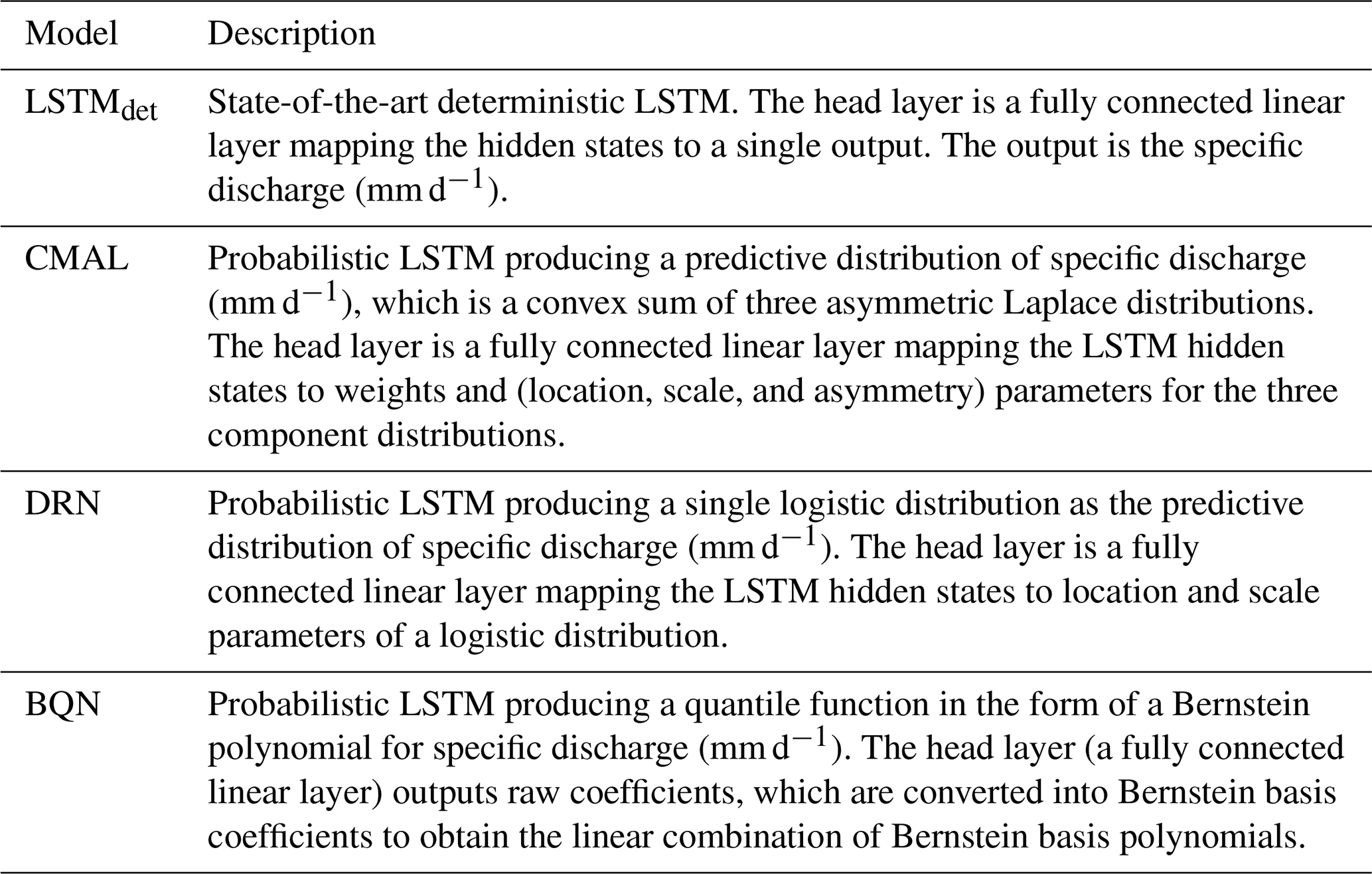
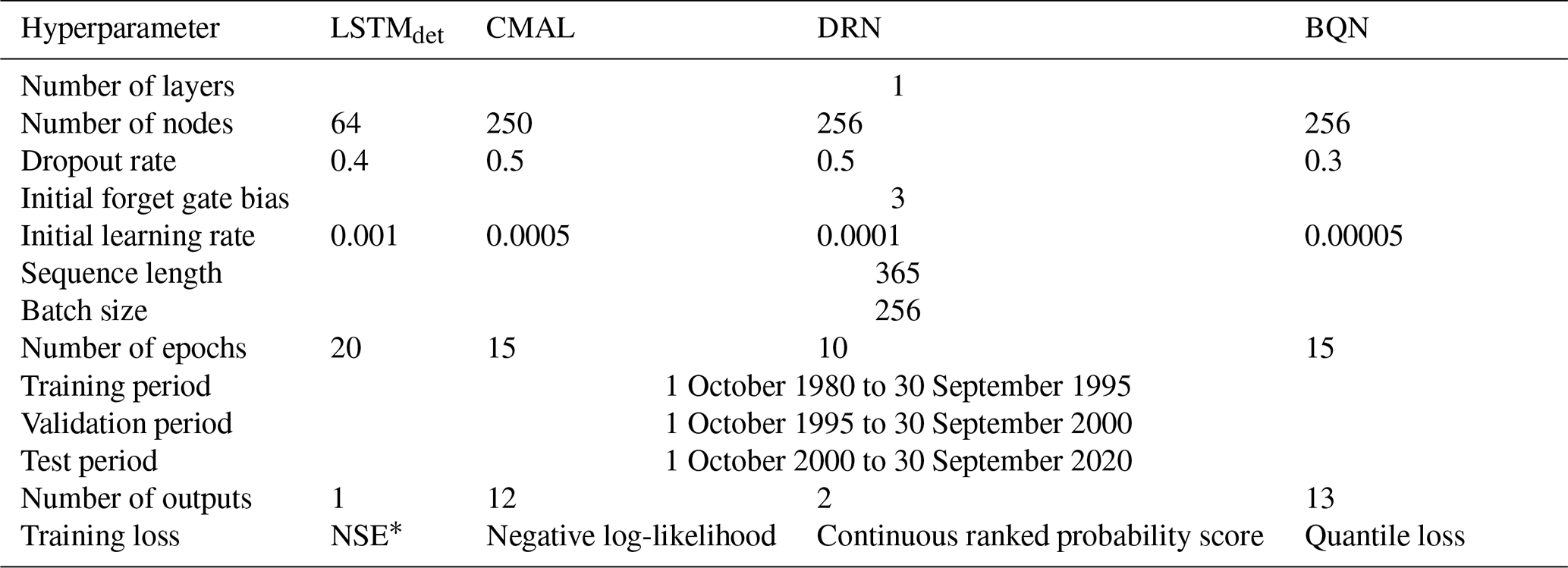
Table 2 Hyperparameters for the models used: LSTM_det, CMAL, DRN and BQN. For details about the hyperparameter selection refer Appendix A.

2.2 Models

The study compares four models, which are all based on the state-of-the-art LSTM. The models have differing head layers, and thus differing outputs, each of which are described in Table 1. Section 2.2.1 to 2.2.4 explain the models further, along with their predictive distributions for the target variable (specific discharge mm d⁻¹). For every model in the study, we train a five-member ensemble to account for stochasticity and random initialization. All models instances are regional; implying that the models are trained collectively on all 196 catchments mentioned in Sect. 2.1. Model implementation is done in PyTorch (Paszke et al., 2019) and optimized using the ADAM (Kingma and Ba, 2017). The training period for all the models extends from 1 October 1980 to 30 September 1995, and the models are tested for the period from 1 October 2000 to 30 September 2020. The sequence length and the batch size are 365 and 256 respectively. All models are initialized with a forget gate bias of 3. A full list of hyperparameters for the three models can be found in Table 2. For brevity, we explain the hyperparameter search in Appendix A and ensemble averaging in Appendix D. A separate validation set (1 October 1995 to 30 September 2000) is used to select the best-performing model for testing. During training, we track each model's validation-period performance using its respective training metric – NLL for CMAL, CRPS for DRN, and quantile loss for BQN. We also generate PIT histograms for the validation period (see Sect. 2.3) and use both the validation-period metric and the associated chi-square statistic to guide model selection.

2.2.1 LSTM_det

The LSTM_det is the state-of-the-art LSTM, as proposed by Kratzert et al. (2019a) and makes deterministic predictions for specific discharge (mm d⁻¹) at each time step. The head layer in the LSTM_det is a fully connected linear layer and maps the hidden states to a single value at every time step. For a detailed description of the LSTM_det, we refer the reader to Kratzert et al. (2019a). The catchment averaged Nash-Sutcliffe efficiency (NSE*) (Kratzert et al., 2019a) is the loss function during training. For every ensemble member, the model parameters from the last training epoch are considered for the test period. The test simulations from the ensemble members are averaged for further analyses.

2.2.2 Countable Mixture of Asymmetric Laplace Distributions

Klotz et al. (2022) implemented the CMAL for the CAMELS-US (Addor et al., 2017) dataset, which predicts a probabilistic distribution for specific discharge (mm d⁻¹) at every time step. Among the four probabilistic models they implemented, the CMAL is the best performing model in terms of the calibration of the predicted distributions. It is state of the art in deep-learning based hydrological uncertainty quantification, and is thus a natural choice for our study. The prediction is a convex sum of three asymmetric Laplace distributions (ALD). An ALD is characterized by location, scale, and asymmetry/skewness parameters, and for three such component distributions, we have a total of nine parameters. To obtain the convex sum, we also require one weight associated with every component distribution. Thus, the LSTM in the CMAL produces 12 outputs. The CMAL is trained by minimizing the negative log-likelihood (NLL) of the observed data with respect to the predicted distribution. The hyperparameters of the CMAL (see Table 2) are adopted from Klotz et al. (2022).

We describe the ALD (see Eq. C1), the mixture distribution (see Eq. C2), and the training loss (NLL; see Eq. C3) for the mixture distribution in Appendix C. Our CMAL implements ALD components where the asymmetry parameter is a real positive value (κ). This differs from Klotz et al. (2022) who implement ALDs characterised by τ – a real value in (0, 1). To model the respective parameter ranges, the κ is modeled using a softplus activation and the τ using a sigmoid activation. We discovered that for the CAMELS-CH dataset, the choice of τ was limiting the CMAL from learning the conditional distributions effectively. We discuss the effects of the CMAL parameterization on the learnt uncertainty representation in Appendix B.

2.2.3 Distributional Regression Network

Fundamentally, the DRN is similar to the CMAL, in that we define the to-be-modeled target distribution and the LSTM estimates its parameters. While CMAL can, in principle, reduce to a single-mixture model, its formulation as a mixture explicitly enables increased expressiveness when supported by the data. In contrast, the DRN is inherently restricted to a single parametric distribution. A comparison between the two highlights a trade-off between structural simplicity and strong inductive bias (DRN) versus high flexibility and data-adaptive distributional shape (CMAL). Thus, the motivation to use the DRN is straightforward: to investigate whether comparable predictive performance can be achieved with analytical and structual simplicity. In principle, a DRN can model any distribution we choose to specify, and the ideal choice is one that closely approximates the true conditional target distribution. Like the ALD, the logistic distribution has heavier tails than the Gaussian, and given its successful application in post-processing weather forecasts (Rasp and Lerch, 2018; Ghazvinian et al., 2021; Schulz and Lerch, 2022; Horat et al., 2024), it is worthwhile to assess its suitability for rainfall–runoff modeling. In the DRN, the LSTM predicts the parameters of a logistic distribution, namely the location and the scale parameters. Training optimizes the Continuous Ranked Probability Score (CRPS, adopted from the scoringrules library; Zanetta and Allen, 2024) of the training data with respect to the estimated predictive distribution. The DRN hyperparameters are mentioned in Table 2 and the hyperparameter search is described in Appendix A. Further mathematical details for the DRN can be found in Appendix C.

2.2.4 Bernstein Quantile Network

The BQN is a nonparametric approach that models the quantile function of the target distribution. Thus, it provides an implicit representation of the underlying distribution that does not require an a priori assumption of the parametric form (Bremnes, 2020). Originally proposed for wind speed forecasting, the BQN has since been applied to a range of target variables, including solar energy (Schulz et al., 2021) and wind gusts (Schulz and Lerch, 2022). Its distributional flexibility makes it a natural candidate for runoff prediction, where the conditional discharge distribution is strongly right-skewed and resists simple parametric characterisation. We include the BQN in this study as it represents an extreme end of the model flexibility spectrum. This quantile function is a linear combination of Bernstein basis polynomials and is given by

$$\begin{array}{}\text{(1)}& Q\left(q\right|\mathbf{x}):=\sum _{l=\mathrm{0}}^d{\mathit{\alpha }}_l(\mathbf{x}\left)B_{l,d}\right(q),q\in [\mathrm{0},\mathrm{1}],\end{array}$$

where α_l(x) are basis coefficients and are a function of the inputs x, and

$$\begin{array}{}\text{(2)}& B_{l,d}\left(q\right)=\left(\genfrac{}{}{0ex}{}{d}{l}\right)q^l(\mathrm{1}-q{)}^{d-l},l=\mathrm{0},\mathrm{1},\mathrm{\dots },d,\end{array}$$

are the Bernstein basis polynomials of degree d∈ℕ for individual quantiles $q\in [\mathrm{0},\mathrm{1}]$.

For a given degree d, the quantile function is fully defined by d+1 basis coefficients. Schulz and Lerch (2022) note that the choice of d is critical, with larger d providing greater flexibility but at the cost of increased estimation variance. We discuss the range of Bernstein polynomial degrees we tested in Appendix A, and adopt a 12th degree Bernstein polynomial. For the BQN, the head layer maps the hidden states of the base LSTM to 13 (12+1) raw coefficients $\stackrel{\mathrm{̃}}{{\mathit{\alpha }}_l}$. One important deviation from Schulz and Lerch (2022) in our implementation is the non-enforcement of strictly positive support for the predicted distribution. This is to maintain consistency with the CMAL and the DRN, where the distributions are similarly not truncated at zero. More generally, such truncation can be considered an inductive bias, whereas one might instead expect the model to learn the true minimum of the data directly. We therefore allow the first basis coefficient (α₀) to be negative. We maintain the requirement that the remaining basis coefficients are strictly increasing by applying a softplus activation and recursively estimating them as follows:

$$\begin{array}{}\text{(3)}& {\mathit{\alpha }}_{\mathrm{0}}=\stackrel{\mathrm{̃}}{{\mathit{\alpha }}_{\mathrm{0}}},{\mathit{\alpha }}_l={\mathit{\alpha }}_{l-\mathrm{1}}+\text{softplus}\left(\stackrel{\mathrm{̃}}{{\mathit{\alpha }}_l}\right),l=\mathrm{1},\mathrm{\dots },d,\end{array}$$

The BQN is trained by optimizing the average quantile loss (QL) over 99 equidistant quantiles. The QL is a consistent scoring function for the corresponding quantile, and the integral of the QL over the unit interval is proportional to the CRPS (Gneiting and Ranjan, 2011). The QL for a quantile q is given by

$$\begin{array}{}\text{(4)}& {\text{QL}}_q(y_{\mathrm{true}},y_q)=max\left(q\right(y_{\mathrm{true}}-y_q),(\mathrm{1}-q\left)\right(y_q-y_{\mathrm{true}}\left)\right)\end{array}$$

where y_true is the true target value, and y_q is the predicted target quantile q obtained from Eq. (1). Table 2 gives the hyperparameters of the BQN, and the hyperparameter search is described in Appendix A.

2.3 Evaluation of predictive distributions

Gneiting et al. (2007) suggest that the goal of probabilistic forecasting is to maximize the sharpness, subject to calibration. Although they use different terminology, Klotz et al. (2022) evaluate their models similarly based on reliability (calibration) and resolution (sharpness). Calibration is a joint property of the predicted distributions and the observed events, and refers to the statistical consistency between the two, whereas sharpness refers to the concentration of the predicted distribution, and is a property of the predicted distribution alone. Quantitatively, calibration and sharpness can be simultaneously evaluated with proper scoring rules, where lower values indicate better predictive performance (Gneiting and Raftery, 2007). The CRPS is a strictly proper scoring rule and is used in this study to evaluate the probabilistic predictions. For the DRN, the CRPS is computed analytically. For the CMAL, as no closed form solution is available, the CRPS is approximated based on samples. For the BQN, the CRPS is approximated from predicted quantiles. The library scoringrules (Zanetta and Allen, 2024) provides torch-compatible functions for calculating the respective closed-form and approximate CRPS for all our models. The CRPS is calculated for every time step and averaged over the test period for every catchment. We report the mean and the median catchment CRPS as a measure of overall model performance.

For a visual assessment of the calibration alone, we compute the the Probability integral transform (PIT) values by evaluating the predicted cumulative distribution functions (CDFs) at the observed values. We then plot PIT histograms for the entire test period and all catchments combined in Sect. 3.1. For the BQN, we resort to the unified PIT (uPIT; Vogel et al., 2018) as only a set of quantiles is available. We also adopt some metrics from Klotz et al. (2022) to evaluate sharpness of the probabilistic predictions. For every time step we calculate the interquartile and the interdecile ranges. Variance is calculated for 7500 samples (adopted from Klotz et al., 2022) drawn from the predictive distributions. The metrics are presented as a mean aggregation over all catchments for the entire test period. Finally, we evaluate the distributions based on single-point metrics such as the Mean Absolute Error (MAE) evaluated on the median of the distributions and the Root Mean Squared Error (RMSE) evaluated on the mean of the distributions. To align with standard hydrological practice, where overall model performance is primarily assessed on point predictions, we also calculate the Nash-Sutcliffe efficiency (NSE) and the Kling-Gupta efficiency (KGE) (following Klotz et al., 2022). We acknowledge that the NSE and KGE are not consistent scoring functions (Vrugt, 2024) and as such, no functional of the predicted distributions minimises either. However, for every time step, the mean of the probabilistic predictions is considered as a point estimator to calculate these metrics and we report the aggregated metrics for the entire test period.

2.4 Flood Risk Communication Agent (FRiCA)

A reinforcement learning episode consists of an agent observing a state s, selecting an action a, and receiving a scalar reward r(a,y), where the reward depends on the chosen action and the realised true severity y. In our application, the state describes the current hydrological situation and the action corresponds to issuing a warning. As only a single warning decision is required, each episode terminates immediately after the action is taken. We created episodes for the FRiCA by running the CMAL over 40 years (1 October 1980 to 30 September 2020). We split these into training (1 October 1980 to 30 September 1995), validation (1 October 1995 to 30 September 2000) and testing episodes (1 October 2000 to 30 September 2020). Excluding median and low flows, we focus on episodes when the predictive probability of exceeding HQ2 (flood with an annual recurrence interval of 2 years) is at least 15 %, making a total of 2441 training, 822 validation and 1696 testing episodes. For every catchment, design floods with annual return intervals of 2, 10, 30, 100, and 300 years are obtained from BAFU (2024). These return-period thresholds are used to classify the observed specific discharge into one of six severity classes, $y\in \mathit{\{}\mathrm{0},\mathrm{1},\mathrm{2},\mathrm{3},\mathrm{4},\mathrm{5}\mathit{\}}$ – y=0 indicates no design-flood threshold was exceeded, and y=1 through y=5 correspond to the HQ2 through HQ300 thresholds. The state s that the agent observes is a 7 d sequence of predictive distributions and 1 d lagged discharge. Thus, in every episode, the agent receives a 7×13 state matrix; the twelve parameters of the CMAL distribution (mixture weight π_i, location μ_i, scale b_i, and asymmetry κ_i for each of three mixture components, $i=\mathrm{0},\mathrm{1},\mathrm{2}$) together with the lagged discharge. This mimics a scenario where the warning-issuing authority is given a predictive distribution, historic hydrological context, and should issue a warning. The action space is discrete, $a\in \mathit{\{}\mathrm{0},\mathrm{1},\mathrm{2},\mathrm{3},\mathrm{4},\mathrm{5}\mathit{\}}$, corresponding to the six severity classes described above.

The reward is a distance-based function of the issued warning a and the true severity y: a correct prediction is rewarded, whereas an incorrect one is penalised in proportion to its ordinal distance from y, scaled by a class weight and, independently, by separate penalty rates for under- and over-warning. Class weights compensate for the imbalance in the frequency of warning classes. The full reward formulation is given in Appendix E. We evaluated nine reward configurations, summarised in Table E1. Unless stated otherwise, the results presented in this paper are for the reward configuration ℛ_UH200,ON. The reward configurations are designed to represent a range of plausible operational preferences rather than to exactly reproduce socioeconomic costs. This enables a systematic investigation of how different reward structures influence the learnt policy and demonstrates that the RL agent adapts its warning behaviour in a consistent and risk-aware manner to changing operational objectives.

FRiCA is implemented in a gymnasium environment (Towers et al., 2025), and trained and evaluated using Proximal Policy Optimization (PPO) (Schulman et al., 2017) algorithm from Stable Baselines3 (Raffin et al., 2021). For evaluation, we divide events into three categories based on true severity y: no floods (class 0), floods (class 1), and extreme floods (classes 2–5). Model selection is performed on the validation set, where the epoch maximising the total number of hits across classes 1–5 is retained for testing. For classes 1–5, a prediction is counted as a hit if the issued warning matches the true severity class, a miss if the issued warning is lower than the true severity, and a false alarm if it is higher. If the issued warning matches the true prediction class 0, it is a true negative. We compare FRiCA-issued warnings against two static baselines: the 99th percentile of the CMAL predictive distribution, and the LSTM_det as a deterministic rule. Results for the reward configuration ℛ_UH200,ON are reported in Table 5, with the full comparison across all reward configurations given in Table E1.

3 Results

In this section, we present the overall evaluation for the probabilistic models based on the CRPS, PIT histograms, resolution metrics and single-point accuracy metrics. Section 3.2 follows with a comparison of the model performance for representative flood events recorded in Switzerland. Finally in Sect. 3.3 we present the results from the FRiCA.

3.1 Global Model Performance

As mentioned in Sect. 2.3 we calculate the mean CRPS for the entire test period per catchment and begin this section by examining the mean and median CRPS across catchments. The CMAL has the lowest mean CRPS of 0.50 as compared to the DRN (0.53) and the BQN (0.56) and outperforms the two models in terms of overall prediction calibration and sharpness. The difference in performance is further pronounced if we consider the median CRPS across all catchments. For the CMAL the median CRPS is 0.39, whereas the DRN and the BQN predictions have a median CRPS of 0.41 and 0.43 respectively. The superior performance of the CMAL can be attributed to its ability to model asymmetry and multimodality in probabilistic runoff predictions. For all the three models, the mean CRPS across all catchments is bigger than the median CRPS, indicating a right-skewed distribution of per-catchment CRPS for all the models. For a plot of the cumulative density function (CDF) of the catchment-wise CRPS refer Appendix F.

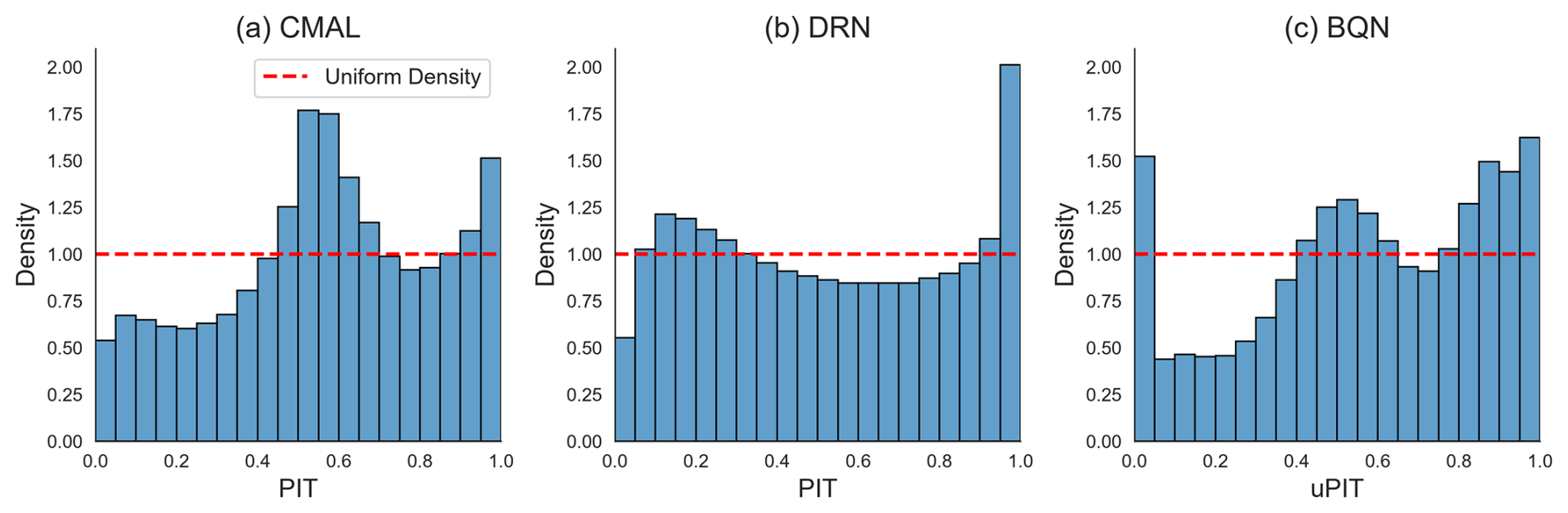
Figure 1 PIT histograms for the (a) CMAL, the (b) DRN and the (c) BQN. The x axes indicate the PIT values from the entire testing data ($\approx \mathrm{1.27}\times {\mathrm{10}}^{\mathrm{6}}$ values) binned into 20 equal-sized bins. The y axes give the density of these bins. The red dashed line indicates the uniform distribution – a case of perfect calibration. Bins with density less than 1 imply that the model predicts the probabilities of occurrence within this bin less frequently than actually observed. Similarly, bins with density more than 1 indicate that the model assigns these probability values more frequently than actually observed.

Figure 1 presents the PIT histograms for the (a) CMAL, the (b) DRN and the (c) BQN aggregated over all catchments. None of the models show perfect calibration and the normalised chi-square test statistics for the three models are 0.14 (CMAL), 0.08 (DRN) and 0.15 (BQN). More importantly, the deviations from the red dashed line in Fig. 1 indicate generally over-dispersed distributions for the CMAL, biased for the DRN and a combination of biased, under-dispersed distributions for the BQN. The CMAL predicts the probabilities in the interval (0.5, 0.6] 1.75 times more than observed, partially causing the under-population of the lower bins. The CMAL distributions are not truncated at zero, implying that some probability mass can extend into the negative space for certain events. This causes the lower probabilities associated with this part of the distribution never being assigned as a PIT value, since observed specific discharge is always positive. This contributes to the probabilities in the intervals (0.0, 0.4] being predicted less often than observed. Probabilities higher than 0.9 are predicted about 1.63 times more, indicating that distributions for some time steps are either biased or under-dispersed. A single distribution (DRN) on the other hand, shows starkly different calibration. The under-population of the first bin, is again a result of the distributions not being truncated at zero. Over-all the DRN distributions match the frequency of observed probabilities closely, but probabilities greater than 0.95 are predicted twice as frequently as observed. This is indicative of under-dispersed distributions for these events and likely an underprediction of high flows. We observe underdispersion in BQN predictions as well, but this affects the representation of lower probabilities more than the higher. The over-population of the first bin is in part an artefact. uPIT calculation for the BQN is based on a uniform quantile grid in the interval [0.01, 0.99] and observations falling out of this range are directly assigned a uPIT value of 0 or 1. Lower probabilities in the interval (0.0, 0.05] are predicted roughly 1.7 times more than observed. Having said that, the training dynamics of the BQN have a particular effect on the BQN calibration. We discuss the reasons for such a PIT distribution for the BQN in Sect. 4.1. For comparison, we also plot probability plots following Klotz et al. (2022) and present them in Appendix F.

Table 3 Metrics indicating sharpness of the predictive distributions (best performing in bold). All metrics are reported as averages over the test period and all catchments. All metrics can take values in the interval (0, ∞) and lower values are better for all metrics.

Table 4 Evaluation of different single-point accuracy metrics (best model in bold). The LSTM_det predictions are determninistic and are as such single-point. For the probabilistic models, the median of the predictive distributions is used to calculate the MAE, and the mean is considered for calculating the RMSE, the NSE, and the KGE. The metrics are calculated for every time step and averaged over the test period for every catchment. The median catchment metrics are reported here.

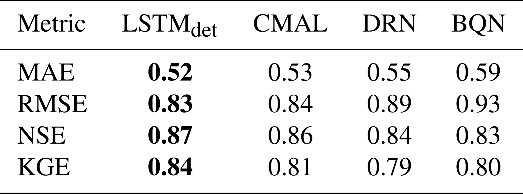
To complement the calibration evaluation of the probabilistic predictions based on the PIT histograms, Table 3 reports the resolution metrics for the probabilistic models. The overdispersed CMAL distributions have the highest variance of 2.63 compared to 1.80 and 1.81 for the DRN and BQN respectively. This pattern holds across all resolution metrics. The DRN and BQN show very similar sharpness overall, though the slightly wider interquartile and interdecile ranges from the BQN suggest that the Bernstein polynomial quantile function learns slightly more dispersed distributions than the DRN. Table 4 reports single-point accuracy metrics for all four models, with the LSTM_det ranking first across all four metrics. The CMAL comes close to the LSTM_det, with an NSE of 0.86 against 0.87 for the LSTM_det and a KGE of 0.81 against 0.84. The DRN and BQN lag further behind, with NSE values of 0.84 and 0.83 and KGE values of 0.79 and 0.80 respectively. We note that results based on computing NSE/KGE from the mean of the predictive distributions should be interpreted with care (Vrugt, 2024). The MAE follows the same ranking, with the BQN median deviating most from observations (0.59) and the CMAL median closest to the LSTM_det (0.53 vs. 0.52). That the CMAL single-point metrics remain competitive despite its overdispersion suggests that its distributional mean and median are well-centred, even if the spread around them is excessive.

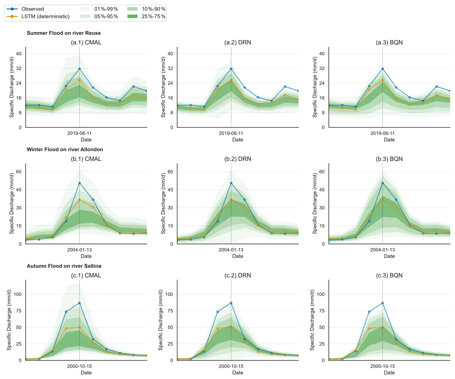
Figure 2 Probabilistic predictions for selected floods recorded in rivers (a.1 to a.3) Reuss in summer, (b.1 to b.3) Allondon in winter, and (c.1 to c.3) Saltina in Autumn. The subplots are in 3×3 grid, with columns representing probabilistic models and rows representing flood events. The x axis is for time and the discharge is plot on the y axis. The blue solid line shows the observed hydrograph and the orange represents the deterministic LSTM_det prediction, both at daily resolution. The predictive distribution is bounded by the 1st and the 99th quantile and darker shades of green represent inner quantiles. For clarity, only the date of the observed flood peak is highlighted, and the hydrographs extend over a 10 d window around the oberved flood peak.

3.2 Probabilistic predictions for representative floods in Switzerland

Figure 2 shows three representative flood events together with their corresponding predictive distributions and the LSTM_det predictions. The selected events span different seasons and were recorded at diverse locations across Switzerland.

Panels (a.1) to (a.3) in Fig. 2 show a summer flood recorded at the Seedorf gauge on the river Reuss. The associated catchment is a high altitude alpine catchment located close to Luzern. The average catchment elevation is about 2000 m above sea level and its area is about 800 km², out of which 6.4 % is glaciated. The event shown here recorded a total rainfall of about 132 mm during the period from 9 to 12 June 2019. On the 10 June, a total rainfall of 102 mm was recorded, which represents a precipitation event with an annual return interval of 30 years (MeteoSwiss, 2022). The resulting flood had a peak specific discharge of 32 mm d⁻¹ recorded on 11 June. The LSTM_det prediction follows the rising limb of the observed hydrograph quite well, until it underestimates this peak flow by 6 mm, and this bias is carried forward throughout the recession. All three probabilistic LSTMs however assign a finite probability of occurence to the observed flood peak, and all within the 99th percentile. The general trend observed in Fig. 1 and Table 3 is evident at an event level: the CMAL predictions are wider than the DRN and the BQN predictions. Moreover, the wider CMAL predictions also capture the smaller flood peak on 15 June within the 95th percentile as against the DRN and BQN predictions which predict the peak close to the 99th percentile. The dispersion from the three models also affects the representation of the rising limb for the event on 11 June. While both the DRN and the CMAL place the observed discharge on this day between the 75th and the 90th percentiles, the BQN places it beyond the 90th percentile. Such comparison is especially valuable from a decision making perspective as days leading to a flood matter equally, if not more.

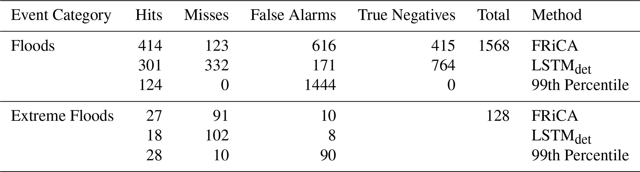
Table 5 Comparison of correct (hits), misses and false warnings for floods and extreme floods given by FRiCA. The warnings are compared to those in the case of discrete LSTM_det predictions and an arbitrary choice of the 99th quantile of the CMAL predictive distributions.

The second flood shown in panels (b.1) to (b.3) in Fig. 2 is a winter flood recorded at the Dardagny, Les Granges gauge on the river Allondon. The catchment is a small, low altitude catchment with an area of 119 km² and mean elevation of about 760 m above sea level. It is located in south-west Switzerland near Genève. From 10 to 14 January 2004, a total of 141 mm of rainfall was recorded at the gauge. Rainfall accumulation on 12 January (49 mm) and 13 January (56 mm) was close to the 2-year return precipitation in the area (MeteoSwiss, 2022). The peak discharge for the resulting flood was about 51 mm d⁻¹. This is almost comparable to a flood estimated to occur once in 10 years (HQ10) at this gauge. The LSTM_det prediction for the peak discharge is 37 mm d⁻¹. Once again, probabilistic predictions successfully capture the flood peak within the 99th percentile. While the CMAL and the DRN place the observed peak between the 95th and the 99th percentiles, the BQN predictions are more confident and place the event close to the 90th percentile. In the days leading up to the flood peak on 13 January, it is worthwhile to note that the DRN predictions extend into the negative space. This is because, the distributions are not truncated at zero and since they are symmetric, in order to capture the flood peak, the lower quantiles extend beyond zero. This is not observed for the CMAL or the BQN as both have in-built flexibility which provides for asymmetry.

The third flood shown in Fig. 2c.1 to c.3 was recorded at the Brig gauge on the Saltina river. The associated catchment is a small alpine catchment and is located in southern Switzerland. During the period from 12 to 15 October, a total rainfall of 435 mm was recorded at the Brig gauge. The rainfall accumulation on 13 and 14 October was more than that estimated to occur once in 100 years (MeteoSwiss, 2022). It rained about 160 mm on the 2 d, which indicates extreme precipitation over two consecutive days. The resulting flood was an HQ30 flood, meaning that the flood peak value is estimated to occur once in 30 years and is about 87 mm d⁻¹. The LSTM_det peak prediction of 50 mm largely underestimates the observed flood. The BQN predictions show a consistent underestimation for 14 and 15 October, leading to an underestimation of total flood volume, and the 99th quantile misses the flood peak by 10 mm. The CMAL and the DRN capture the flood peak on 15 October close to ther 96th and 99th percentile respectively. The 99th percentile from the CMAL prediction for this day is 117 mm, well above the observed flood peak and indicates a long tail. Similar observations can be made for 14 June, where the CMAL predictions have a long tail extending up to 115 mm, but the DRN predictions are shorter with the observed discharge being placed at the 98th percentile.

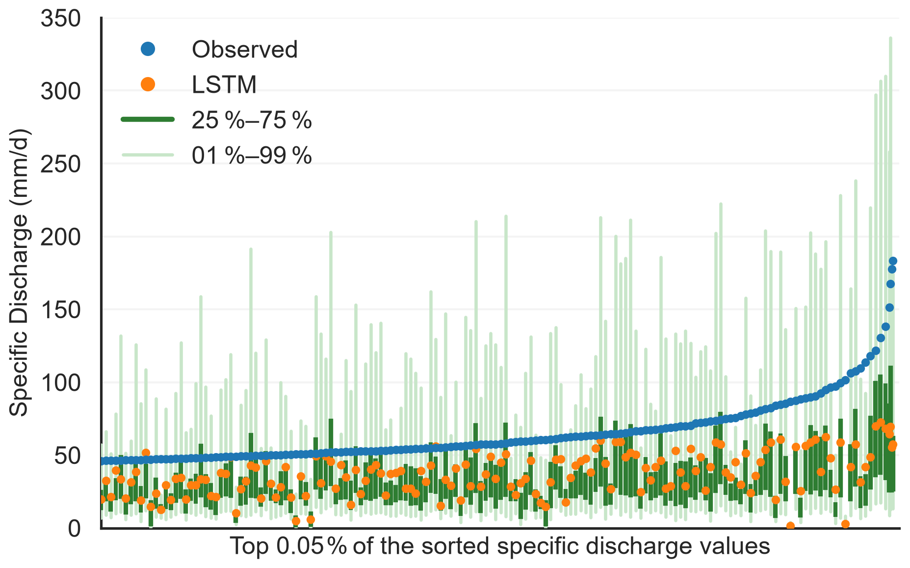
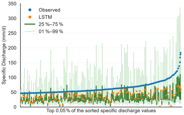
Figure 3 Selected observed discharge values from the top 0.05 % tail (635 discharge values) of the testing distribution, sorted in increasing order (blue dots); for legibility, every fourth value is shown. The corresponding LSTM_det predictions are shown by orange dots. The IQR for the CMAL predictive distribution is shown as a dark green line, and the range between the 1st and 99th quantiles is shown as a light green line.

In summary, Fig. 2 highlights the performance gain from probabilistic predictions for high-stakes rare events. This is not limited to the representative flood events from Fig. 2. One of objectives of this study is to establish the advantage of probabilistic predictions for tail regions of the discharge distribution. To explicitly examine model performance in the extremes, Fig. 3 shows selected observed discharge values from the top 0.05 % of the sorted test-period discharge (635 values in total). The maximum observed discharge during the testing period is about 180 mm d⁻¹ (the largest flood in CAMELS-CH). The LSTM_det simulations underestimate about 97 % of these values, with a mean underestimation of about 28 mm d⁻¹. The figure also shows the CMAL predictive distributions for every observation, and about 83 % of the observed values are within the 99th quantile of their respctive predictive distributions. The maximum 99th percentile from the CMAL predictions is 336 mm d⁻¹. The DRN and the BQN distributions, owing to their under-dispersed distributions, capture about 60 % and 57 % of the values from Fig. 3 within their 99th percentile. The maximum 99th percentile from the these models is 125 and 140 mm d⁻¹ respectively. We discuss these results highlighting the trade-off between probabilistic calibration and accuracy in Sect. 4. However, they underscore the potential advantage of probabilistic LSTMs for flood modelling as they can represent a broader range of possible outcomes and assign non-zero probability to extreme floods that deterministic predictions tend to underestimate.

3.3 FRiCA based flood warnings

Table 5 compares hit, miss, and false alarm counts for FRiCA against the LSTM_det and the 99th percentile rule across flood and extreme flood episodes. For floods, FRiCA achieves the highest hit count (414), outperforming the LSTM_det (301) and the 99th percentile rule (124). This comes at the cost of a higher false alarm count (616) compared to the LSTM_det (171), reflecting a more aggressive warning posture. The 99th percentile rule, by contrast, issues no missed events but generates an extremely high number of false alarms (1444), rendering it operationally impractical.

For extreme floods (HQ10 and above), the picture is more constrained by the rarity of events (128 total). FRiCA again achieves a higher hit count (27) than the LSTM_det (18), while the 99th percentile rule captures the most events (28) but again at the expense of the highest number (90) of false alarms. FRiCA maintains a more favourable false alarm count (10) in this category, comparable to the LSTM_det (8). Overall, the reinforcement approach (FRiCA) demonstrates a learned trade-off between sensitivity and specificity that neither of the two static rules achieves: it detects more flood events than the LSTM_det while avoiding the excessive false alarm rate of the 99th percentile rule.

4 Discussion

We frame the discussion around the three research questions stated in the introduction to this paper (see Sect. 1).

4.1 Which of the investigated probabilistic LSTMs provides the most reliable rainfall–runoff simulation?

None of the investigated probabilistic models achieves perfect calibration for the Swiss catchments. That is, each one exhibits distinct patterns of miscalibration. Nevertheless, perfect calibration is not a prerequisite for addressing the main objective of this work (i.e. to establish the need for probabilistic LSTMs for improved flood forecasting). If a preferred direction of miscalibration exists, it is over-dispersion, as this implies a conservative, better-safe-than-sorry stance for warning systems. Over-dispersed distributions, such as the CMAL distributions, mean that the system is prepared, or over-prepared, more often than strictly necessary. Thus, despite having room for improvement in terms of calibration, the current model performance is sufficient to address our second and main research question. In terms of single-value metrics, all probabilistic models approach the deterministic LSTM NSE, with the CMAL yielding the best NSE among the three probabilistic models, corroborating the findings of Klotz et al. (2022), who reported only slight differences between the CMAL and the deterministic LSTM for CAMELS-US. We acknowledge that the NSE is not a consistent scoring function (Vrugt, 2024) and should not be used to evaluate the performance of probabilistic models, whose primary objective is to represent predictive uncertainty. Nevertheless, we include NSE because it is well established within the hydrological community and allows readers to benchmark the probabilistic models against the large body of existing deterministic rainfall–runoff studies.

The DRN exhibits the best calibration among the three probabilistic models despite its structural simplicity, with only slight underdispersion. Our findings are in line with Schulz and Lerch (2022), who systematically compared probabilistic machine learning approaches for wind gust forecasts in Germany and showed that the DRN achieved the best performance at 55 % of stations, followed by the BQN at 37 %. This advantage may be attributed to the use of a single logistic distribution, the CRPS loss function, or the interaction of both. Comparing a single DRN trained with CRPS against one trained with NLL reveals similar patterns of miscalibration in both cases, that the uppermost PIT bin is overpopulated and slight miscalibration persists in the lower bins. Adopting a truncated logistic distribution successfully resolves the miscalibration in the lower PIT bins, though it has limited effect on the overpopulation of the uppermost bin, suggesting that the upper-tail miscalibration reflects a structural limitation of the logistic family rather than a consequence of the loss function. During training, we observed that the CRPS loss can at times prioritise sharpness at the expense of calibration, a tendency documented empirically and theoretically by Buchweitz et al. (2025). However, in a correctly specified model, CRPS-based parameter estimation is consistent and the resulting distribution will be calibrated. The residual underdispersion in the DRN may therefore reflect model misspecification inherent to the logistic distribution assumption rather than a fundamental limitation of the CRPS loss itself. Future work could explore alternative parametric families, such as the asymmetric Laplace or log-normal distributions, to better accommodate the heavy-tailed, positively skewed streamflow distributions characteristic of the Swiss catchments.

The BQN offers considerable flexibility by directly estimating the quantile function without requiring an a priori assumption about the shape of the conditional target distribution (Bremnes, 2020). The support of the BQN distribution is determined entirely by the boundary coefficients, spanning [α₀,α₁₂], meaning the range and internal shape of the predictive distribution are both encoded in the learned Bernstein coefficients. Monotonicity of the quantile function is enforced via a softplus activation function, such that ${\mathit{\alpha }}_{\mathrm{0}}\le \mathrm{\cdots }\le {\mathit{\alpha }}_{\mathrm{12}}$. Consequently, the spread of the predictive distribution is governed entirely by the magnitude and spacing of these increments. The observed underdispersion in the BQN forecasts can be attributed to a failure to learn adequate coefficient spacing across the highly skewed streamflow regime. When the model cannot distribute probability mass appropriately across the full dynamic range of the training data, it is forced into a compensatory strategy, where the lower-order coefficients are inflated to ensure the support [α₀,α₁₂] spans observed high flows, rather than being anchored near the low-flow baseline. This inflation compresses the effective spacing between lower coefficients, collapsing resolution precisely in the low-flow regime and resulting in a considerable fraction of low flows being assigned probability mass beyond the first quantile. Whilst the BQN's non-parametric flexibility is theoretically appealing, for datasets with high variability, special attention should be given to the raw coefficients to fully exploit this flexibility.

The study uses three different loss functions across the three models. Although all are proper scoring rules, the NLL and the CRPS can penalise misrepresentation of variance differently depending on the estimated distribution, and the three losses penalise tail miscalibration differently. Our choice of losses for the three models limits our ability to separate the respective impacts of loss functions and the assumed distributions. Although we assess the global model calibration, a systematic comparison of probabilistic models based on distributions and loss functions is not central to this study. As with the calibration considerations above, the choice of loss or the evaluation metric is not a limiting factor in addressing our main research objective. Modellers can always choose to train a single network with multiple heads and losses so that its internal representation considers multiple characterisations of aleatoric uncertainty simultaneously (Buchweitz et al., 2025). We leave it to future work to examine whether such an approach would yield synergistic effects or whether it must be treated as a multi-objective optimisation problem.

4.2 Why are probabilistic LSTMs more suitable to represent hydrological extremes and the tail regions of the marginal discharge distribution?

Catchments are, in principle, deterministic dynamical systems in which rainfall–runoff generation is a deterministic process. If all relevant system states were fully observed, the governing dynamics perfectly known, and both inputs and targets free of measurement error, a probabilistic formulation would be unnecessary. In practice, however, none of these conditions are met. Hydrological modelling relies on spatially aggregated forcing data and discharge observations that are affected by measurement uncertainty, representativeness errors, and unresolved sub-grid-scale processes. As a result, the conditional relationship between meteorological forcing and runoff is inherently uncertain and often highly skewed. This can be illustrated by a simple example from CAMELS-CH: during the training period, precipitation events of approximately 100 mm d⁻¹ occurred 27 times, yet floods exceeding 40 mm d⁻¹ were observed in only 6 of these cases. Conversely, floods can also occur without extreme precipitation, for example through rain-on-snow events or highly saturated antecedent conditions. Although this example deliberately neglects many hydrologically relevant variables, it highlights a fundamental limitation of the training data: the predictors available to the model do not uniquely determine the observed runoff response. As a result, the LSTM is effectively trained on a conditional distribution of plausible discharges rather than a single deterministic outcome.

Deterministic LSTM simulations tend to underestimate these tail events because the model learns to represent the conditional mean of the target distribution. By collapsing the conditional distribution to a single predicted value, the deterministic LSTM cannot adequately represent the rare but physically plausible runoff responses that constitute the upper tail and that might have been in training. Adaptations to deterministic loss functions offer a partial remedy: strategies such as weighting schemes within least-squares objectives or transformation of the target variable have been proposed to improve representation of extreme flows (Thirel et al., 2024). However, Thirel et al. (2024) note that transformations targeting extreme flows well tend to be less robust across other flow regimes. Though we did not replicate streamflow transformation experiments for the deterministic LSTM, we observed analogous behaviour for an adapted MSE loss (Baste et al., 2025): performance on extreme flows improved at the cost of global skill. Similarly, optimising for a higher quantile through quantile or expectile losses can improve metrics focused on high flows, such as FHV, but typically increases false alarms and leads to systematic overestimation of median and low flows. In essence, such strategies require a trade-off between sensitivity to extremes and overall predictive reliability, often necessitating multiple models calibrated for different objectives. Probabilistic LSTMs that estimate the entire conditional discharge distribution offer a more principled alternative, providing information across all flow regimes within a single model.

The three flood events shown in Fig. 2 illustrate how these conceptual differences manifest in practice. For the summer flood at Seedorf (panels a.1–a.3), the deterministic LSTM reproduces the overall hydrograph shape but underestimates the peak discharge, whereas the probabilistic LSTMs capture the event within their upper predictive quantiles. The highly extreme Alpine flood at Brig (panels c.1–c.3) further accentuates this contrast, with the deterministic LSTM severely underestimating the peak while the probabilistic LSTMs place the observation within their upper tail. Across all cases, probabilistic models do not eliminate errors entirely – particularly for the most extreme peaks or total volumes – but they consistently broaden the range of plausible responses in a physically meaningful way. These results underscore that the principal benefit of probabilistic formulations lies not in improving median predictions, but in providing a structured and interpretable representation of uncertainty under extreme forcing conditions. Importantly, this additional information comes at little practical cost, as the probabilistic LSTMs require only marginally more parameters and computational effort than their deterministic counterpart while providing substantially richer information for flood-risk assessment and decision-making.

Importantly, this behaviour is not limited to a few selected events. As shown in Fig. 3, approximately 83 % of the highest discharge values (top 0.05 % of the sorted record) are captured within the 99th percentile of the CMAL distributions. Expecting full coverage of this region, or expecting these extreme values to fall within narrow confidence intervals, is at odds with the principles of probabilistic calibration. Under probabilistic calibration, predicted and observed conditional probabilities are equal. If the true conditional probability of some event lies beyond the 99th percentile, expecting it to be predicted within lower quantiles is inconsistent with this definition. In other words, an expectation that all data lies within the 99th quantile, implies particular bins from the PIT histogram will be empty, causing overpopulation in the lower bins, and thus leading to miscalibration. The difference in upper-tail coverage between the CMAL and the DRN is a direct consequence of their respective calibration characteristics. The over-dispersion of the CMAL pushes its 99th percentile beyond the most extreme observed values. Although this leads to global miscalibration, it is superficially appealing from a coverage perspective, and perhaps desirable from an operational standpoint.

The LSTM saturation effect documented by Baste et al. (2025) for deterministic models may also occur in our probabilistic setting, though its severity might differ across models. In the deterministic case, saturation of the LSTM's internal state at high discharge values causes underestimation of peak flows, as the network's gating mechanism loses sensitivity in the high-flow regime. In the probabilistic case, an analogous saturation effect would affect the distribution parameters of the CMAL and the DRN, and the raw Bernstein coefficients of the BQN. Ultimately manifesting as a failure to assign sufficient probability mass to extreme discharge values. For the BQN and DRN, whose predictive distributions are already underdispersed, such saturation would compound the existing upper-tail miscalibration. For the CMAL, however, the effect might not be so severe. The over-dispersed predictive distributions already assign considerable probability mass to extreme discharge values, so any reduction in upper-tail sensitivity due to LSTM saturation is absorbed within the existing excess spread. Saturation is therefore unlikely to materially affect flood warning performance for the CMAL, whereas for the BQN and DRN it represents an additional source of upper-tail underestimation that warrants dedicated investigation in future work.

Taken together, our findings and the findings of our previous study (Baste et al., 2025) suggest that the principal limitation in extreme flood prediction may not lie in the specific neural-network architecture or loss function, but rather in the information content of the data available for training. When the predictors do not uniquely determine the runoff response in a regional model training, any deterministic model is forced to collapse a distribution of plausible outcomes into a single prediction. Architectural modifications, alternative loss functions, and targeted training strategies may alleviate this issue to some extent, but they cannot fundamentally resolve the ambiguity inherent in the input–output relationship. In contrast, probabilistic models explicitly acknowledge this uncertainty by estimating the full conditional discharge distribution. Consequently, we argue that future improvements in flood prediction will likely depend on two complementary developments: more informative data that better constrain the hydrological state of the catchment, and probabilistic modelling frameworks capable of translating the remaining uncertainty into actionable predictions. Together, these advances provide a pathway not only towards improved representation of extreme floods, but also towards data-driven warning systems in which warning thresholds and decision rules can be learned directly from calibrated predictive distributions rather than being imposed a priori.

4.3 Can reinforcement learning aid operational flood-warning communication by learning a risk-aware translation of predictive distributions into actionable warnings based on flood-intensity categories?

The FRiCA results are promising and demonstrate its potential as a novel decision layer within early flood warning systems. Across all explored reward configurations, FRiCA consistently learns policies that reflect the structure of the reward signal. We demonstrate that FRiCA acquires a risk-aware, reward-based rule for issuing warnings rather than a fixed heuristic. This stands in meaningful contrast to current operational practice, where the translation from a probabilistic forecast to a categorical warning level remains largely dependent on expert judgment. In Switzerland, for example, flood hazard is communicated via a five-level danger scale (Federal Office for the Environment (FOEN), 2026), but the assignment of a level still relies on a forecaster's interpretation of multiple hydrological and meteorological models rather than on an optimized or learned rule. Certain formalisations exist – such as minimising a cost-loss ratio (Roulin, 2007) or counting ensemble-member exceedances against a threshold (Dietrich et al., 2009) – but these are static, analytically-driven, computed a priori, and not updated from observed outcomes. FRiCA addresses this gap by framing warning communication as a decision problem with outcome-based rewards, the agent can in principle be updated in real time as new flood events are observed and their consequences become known. This closes a feedback loop that static rules cannot close. The adaptability of the learned policy to user-defined risk preferences is further supported by the asymmetric reward experiments. To our knowledge, reinforcement learning applied to the communicative step of translating a predictive distribution into a categorical warning remains largely unexplored in hydrology.

That said, these results should be interpreted as an exploratory proof of concept rather than as a finished operational warning framework. The purpose of FRiCA in this study is to demonstrate that reinforcement learning can, in principle, be used to learn a reward-sensitive decision layer for translating probabilistic flood forecasts into categorical warning decisions. The key step of transitioning from probabilistic model output to an actionable warning, which is often left implicit in forecasting, is addressed by FRiCA. The results therefore highlight potential, but they also make clear that more methodological developments are required before such an approach could be considered operationally robust. For instance, considerable variance across random seeds was observed for all reward configurations, indicating that the learned policies are sensitive to initialisation and that the training signal, particularly for the rarest flood severity classes, is insufficient for consistent convergence. No systematic hyperparameter optimisation was performed, and the policy network configuration and reward weights were chosen pragmatically to demonstrate feasibility rather than to identify an optimal design (see Appendix E). Critically, the results also highlight the risk of reward hacking, whereby an agent achieves high nominal reward through behaviour that satisfies the literal specification of the reward function while failing to capture the designer's actual intent (Amodei et al., 2016; Skalse et al., 2025). In the present case, without explicit accounting for class imbalance or asymmetric penalties, the agent collapses to the dominant class within a few training epochs, achieving a high nominal reward by ignoring rare but consequential events entirely. This underscores that careful reward design is essential, as the quality of the learned policy is fundamentally bounded by how faithfully the reward reflects the true cost structure of flood warning decisions. One avenue for addressing this limitation in future work is inverse reinforcement learning, where instead of hand-specifying a reward function, the reward is inferred from demonstrated behaviour, for instance, historical decisions made by operational forecasters (Ng and Russell, 2000; Ziebart et al., 2008). Such an approach could help recover a reward structure that more faithfully reflects the implicit cost trade-offs forecasters already make in practice, rather than relying on manually designed reward weights. The present study therefore provides a basis for future work to move beyond feasibility and toward operational robustness, in particular through systematic hyperparameter optimisation, reward functions that more explicitly encode the asymmetry between missed events and false alarms (potentially informed by inverse reinforcement learning from forecaster behaviour), and class-balanced episode sampling to strengthen the training signal for rare but consequential severity classes.

5 Conclusion

This study evaluated the performance of three probabilistic LSTMs for rainfall–runoff simulation across Switzerland, with a particular focus on their ability to represent uncertainty for discharge extremes. Specifically, we investigated the extent to which probabilistic predictions provide added value over deterministic simulations, and why such advantages are most pronounced in the tails of the marginal distribution. In addition, we explored a reinforcement learning-based communication method that translates probabilistic runoff forecasts into actionable flood warnings for early warning systems. Based on our findings, we draw the following conclusions:

• The core limitation in extreme flood prediction may lie not in network architecture or loss function, but in the information content of the training data itself. When predictors fail to uniquely determine the runoff response, deterministic models are forced to collapse multiple plausible outcomes into a single point estimate. Probabilistic models, by contrast, estimate the full conditional discharge distribution, offering a more appropriate representation of uncertainty for extreme events and supporting risk-informed decision-making.

• The degree of distributional flexibility assumed by each of the investigated models translates into distinct miscalibration signatures. DRN, the most constrained of the three, mostly exhibits overestimation of the highest quantiles, implying underconfidence for tails of the marginal discharge distribution. CMAL, by contrast, is consistently overdispersed, while BQN tends to overestimate the lowest quantiles. Thus, greater distributional flexibility may not guarantee better calibration.

• Even under perfect calibration, not all specific discharge values fall within the 99th or lower predicted quantiles. This reflects the concepts of calibration and accuracy being at odds with each other. A well-calibrated model is not necessarily the most informative one for decision-making. For extreme events in particular, a degree of overdispersion may be preferable to nominal calibration, since wider predictive bounds provide greater confidence that the true value is captured, even at the cost of sharper, calibrated intervals.

• The reinforcement learning-based agent demonstrates potential as decision-support for early warning systems. By condensing full predictive distributions into actionable warning levels, the agent offers a principled alternative to static rules. Nevertheless, substantial scope for improvement remains, including systematic hyperparameter optimization of the policy network, and better reward design.

Appendix A: Hyperparameter Search

In the following, we explain the basis for the hyperparameters (see Table 2) used for the models in this study. No hyperparameter search was conducted for LSTM_det; its hyperparameters were adopted directly from Baste et al. (2025). Similarly, the CMAL hyperparameters were adopted from Klotz et al. (2022), including the dropout rate of 0.5.

For the DRN, we explored a limited set of hyperparameters, testing two hidden sizes (64, 256) and two learning rates (0.00005, 0.0001). Based on validation-period CRPS and calibration (assessed via PIT histograms) after 10 epochs, we selected a hidden size of 256 and a learning rate of 0.0001.

For the BQN, the degree of the Bernstein polynomial is a critical hyperparameter: higher-degree polynomials offer greater flexibility but also increase predictive variance. Given the computational cost of a full grid search, we fixed the hidden size at 256 and tuned the remaining hyperparameters sequentially. We first tested four polynomial degrees (8, 12, 16, and 20) and found that degree 12 performed best based on validation-period NLL and PIT histograms. We then tested learning rates of 0.01, 0.005, 0.0001, and 0.00005, and selected 0.00005 using the same criteria. Initially, we fixed the dropout rate at 0.5, as with the CMAL and DRN; however, we found that the BQN's learned behaviour was more sensitive to network capacity and dropout than the other models. We therefore tested three dropout rates (0.3, 0.4, 0.5) with the previously selected hyperparameters held fixed, and found 0.3 to perform best.

As the primary objective of this study is not to identify the optimal probabilistic LSTM configuration for CAMELS-CH, our hyperparameter tuning efforts were intentionally limited. We leave a more exhaustive search across the three model architectures to future work.

Appendix B: The choice of CMAL parameterization

We initially implemented the CMAL with the component asymmetric Laplace distributions parameterized by τ, following Klotz et al. (2022) and Brando et al. (2019). We refer to this variant as CMAL_τ throughout this appendix. Here, τ is the asymmetry parameter, taking values in (0,1). From a technical standpoint, we enforce the bounds with a sigmoid activation function. In contrast, the current implementation – a κ-parameterized CMAL (CMAL_κ) – uses the skewness parameter $\mathit{\kappa }\in (\mathrm{0},\mathrm{\infty })$, which can, inter alia, be realized via a softplus activation. The two parameterizations describe the same family of component densities and are related by $\mathit{\tau }={\mathit{\kappa }}^{\mathrm{2}}/(\mathrm{1}+{\mathit{\kappa }}^{\mathrm{2}})$. Hence, they are mathematically equivalent. However, the choice can influence the optimization dynamics.

For mixture component k with a latent state vector z_k and shape parameter τ_k or κ_k, the choice of activation affects the gradient. Under the sigmoid, the gradient decays symmetrically to zero as τ_k approaches 0 or 1. If we want to model a conditional distribution with a component that is highly skewed to one side τ_k will inevitably approach one of these boundaries. And, when a component gets closer to the skew it needs, gradient signal weakens and fails to push it all the way through. This can prevent any one component of the mixture from specialising for large skewness. Under the softplus, the gradient $\partial {\mathit{\kappa }}_k/\partial z_k$ saturates asymmetrically only as κ_k→0 – when κ_k grows, the activation gradient approaches 1 rather than 0.

The activation asymmetry is especially pronounced for extreme high flows (which are by their very nature rarely present in the data). With CMAL_τ, this rare signal is further affected by the weak activation gradient at the very τ_k values needed to act on it. With CMAL_κ, the same rare signal is not weakened: once a component drifts toward larger κ_k, its responsibility for extreme observations rises, raising its contribution to the mixture and further increasing the activation gradient. CMAL_κ does therefore have theoretical properties that can make it easier to optimize for high flows.

Appendix C: Mathematical Basis for the CMAL and the DRN

In this section, we give the mathematical basis for the CMAL and the DRN. We begin with the probability density function for a countable mixture of asymmetric Laplace distributions and the NLL. We then give the closed-form expression for the CRPS for a single logistic distribution. The scoringrules library (Zanetta and Allen, 2024) provides an implementation of the CRPS that is compatible with PyTorch.

The probability density function for a single asymmetric Laplace distribution, parameterized by location μ, scale b, and skewness parameter $\mathit{\kappa }\in (\mathrm{0},\mathrm{\infty })$, is given by

$$\begin{array}{}\text{(C1)}& {\mathcal{A}}_{LD}\left(y\right|\mathit{\mu },b,\mathit{\kappa })={\displaystyle \frac{\mathit{\kappa }}{b({\mathit{\kappa }}^{\mathrm{2}}+\mathrm{1})}}\cdot \left\{\begin{array}{ll}\exp \left[{\displaystyle \frac{y-\mathit{\mu }}{b\mathit{\kappa }}}\right],& \text{if }y<\mathit{\mu },\\ \exp \left[-\mathit{\kappa }{\displaystyle \frac{y-\mathit{\mu }}{b}}\right],& \text{if }y\ge \mathit{\mu },\end{array}\right.\end{array}$$

where κ>1 corresponds to left-skewed distributions, κ<1 corresponds to right-skewed distributions, and κ=1 recovers the symmetric Laplace distribution.

For the CMAL, the weighted sum of three such distributions is given by

$$\begin{array}{}\text{(C2)}& p\left(y\right|\mathbf{x})=\sum _{k=\mathrm{1}}^{\mathrm{3}}{\mathit{\pi }}_k(\mathbf{x})\cdot {\mathcal{A}}_{LD}\left(y\mid {\mathit{\mu }}_k\left(\mathbf{x}\right),b_k\left(\mathbf{x}\right),{\mathit{\kappa }}_k\left(\mathbf{x}\right)\right),\end{array}$$

where the mixture weights (π_k), location parameters (μ_k), scale parameters (b_k), and skewness parameters (κ_k) are outputs from the LSTM, and are thus a function of the inputs x at every time step.

The CMAL is trained by maximizing the log-likelihood of the training data (y_true) under the estimated mixture density conditional on the input; for three components, the negative log-likelihood is given by

$$\begin{array}{}\text{(C3)}& \begin{array}{rl}& {\text{NLL}}_{{\mathcal{A}}_{\mathrm{LD}}}\left(\mathit{\mu }\right(\mathbf{x}),b(\mathbf{x}),\mathit{\kappa }(\mathbf{x}),y_{\mathrm{true}})\\ & =-\log \left(\sum _{k=\mathrm{1}}^{\mathrm{3}}{\mathit{\pi }}_k\left(\mathbf{x}\right)\cdot {\mathcal{A}}_{\mathrm{LD}}\left(y_{\mathrm{true}}\left|{\mathit{\mu }}_k\right(\mathbf{x}),b_k(\mathbf{x}),{\mathit{\kappa }}_k(\mathbf{x})\right)\right).\end{array}\end{array}$$

The DRN is trained by optimizing the CRPS of the training data (y_true) for an estimated logistic distribution ℒ(μ(x),s(x)) conditional on the input x. For a single logistic distribution, a closed-form equation for the CRPS exists:

$$\begin{array}{}\text{(C4)}& \begin{array}{rl}& \text{CRPS}\left(\text{Logistic}\right(\mathit{\mu }\left(\mathbf{x}\right),s\left(\mathbf{x}\right)),y_{\mathrm{true}})\\ & =s\left(\mathbf{x}\right)\left({\displaystyle \frac{y_{\mathrm{true}}-\mathit{\mu }\left(\mathbf{x}\right)}{s\left(\mathbf{x}\right)}}-\mathrm{2}\log F\left({\displaystyle \frac{y_{\mathrm{true}}-\mathit{\mu }\left(\mathbf{x}\right)}{s\left(\mathbf{x}\right)}}\right)-\mathrm{1}\right),\end{array}\end{array}$$

where

$$\begin{array}{}\text{(C5)}& F\left({\displaystyle \frac{y-\mathit{\mu }\left(\mathbf{x}\right)}{s\left(\mathbf{x}\right)}}\right)={\left(\mathrm{1}+\exp \left(-{\displaystyle \frac{y-\mathit{\mu }\left(\mathbf{x}\right)}{s\left(\mathbf{x}\right)}}\right)\right)}^{-\mathrm{1}}\end{array}$$

is the CDF of the logistic distribution. We used the library scoringrules (Zanetta and Allen, 2024) which has a torch compatible implementation of Eq. (C5).

Appendix D: Combining predictive distributions

All results presented in Sect. 3 and subsequent analyses are based on ensemble averages. For the LSTM_det, the ensemble average is the average of the predicted deterministic discharge of individual member models. For the probabilistic models, we adopt the aggregation process implemented by Schulz and Lerch (2022), and since Klotz et al. (2022) use a single member CMAL, we adopt the ensemble averaging logic from the former for the CMAL as well. For the CMAL, the weights of the three component distributions as well as the location, scale, and asymmetry parameters are averaged over the ensemble members. These are then used to calculate the resulting ensemble-averaged discharge distributions. Similarly, for the DRN, the location and the scale parameters from the ensemble members are averaged to produce the ensemble-averaged distribution parameters. For the BQN, the raw coefficients are first converted into Bernstein basis coefficients (according to Eq. 3) for every ensemble member. The basis coefficients are then averaged over the ensemble members and the quantile function is then obtained according to Eq. (1). For a detailed discussion on combining predictive distributions from ensembles of neural network models, see Schulz et al. (2026).

Appendix E: FRiCA: Sensitivity to reward configuration

We adopted a distance based reward for the FRiCA and tested sensitivity to nine reward configurations explained in Table E1. We ran each configuration for three seeds and for three choices of the entropy coefficient, which controls the policy's exploration vs exploitation.

Let w(y)=c_y if class weights c_y are supplied, and w(y)=1 otherwise, and let $d=|y-a|$ denote the ordinal distance between the issued warning a and the true severity y. The reward is

$$\begin{array}{}\text{(E1)}& r(a,y)=\left\{\begin{array}{ll}{r}_{\mathrm{correct}}\cdot w\left(y\right)& \text{if }d=\mathrm{0}\\ -p_{\mathrm{under}}\cdot d\cdot w\left(y\right)& \text{if }a<y\text{(under-warning)}\\ -p_{\mathrm{over}}\cdot d\cdot w\left(y\right)& \text{if }a>y\text{(over-warning)}\end{array}\right.\end{array}$$

Table E1 Reward configurations and resulting Hit (H), Miss (M), and False Alarm (FA) counts by warning severity category for ten reward configurations. For each PPO reward configuration, the best-performing seed under entropy coefficient 0.10 is reported. The asterisked ℛ_UH200,ON* row corresponds to the configuration used for the main results in Table 5; the unmarked ℛ_UH200,ON row above it reports results from the best seed for comparison.

Appendix F: CDF for CRPS and PIT histograms with probability plots

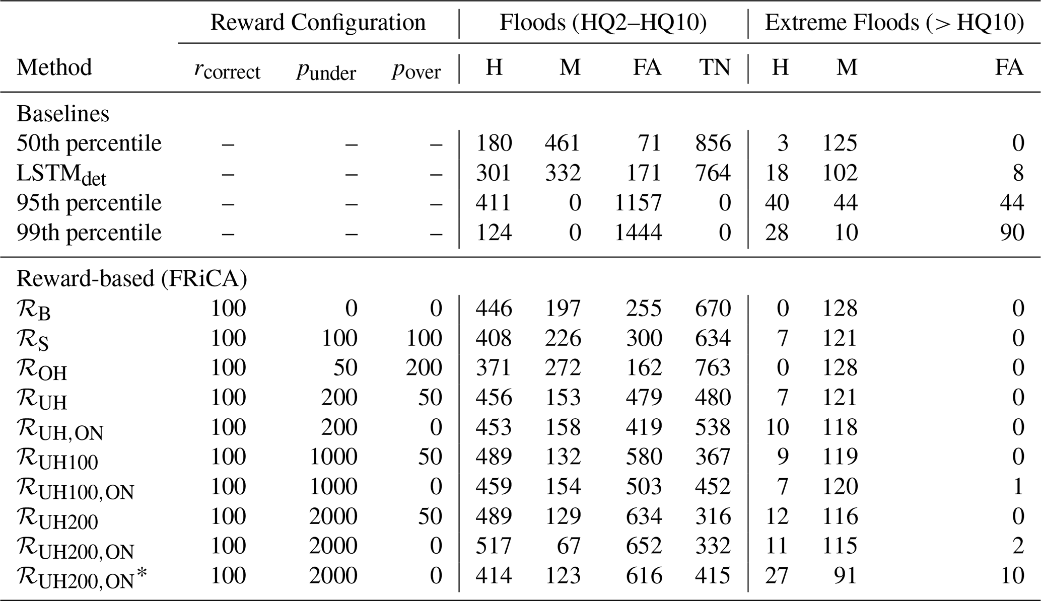
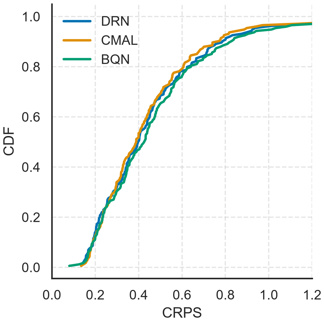
Figure F1 Cumulative density function (CDF) of Continuous ranked probability score (CRPS) for CMAL, DRN and BQN predictions (lower values are better). The CRPS is calculated for every catchment and averaged over the test period. The median CRPS from the three models is 0.39, 0.41 and 0.43 respectively.

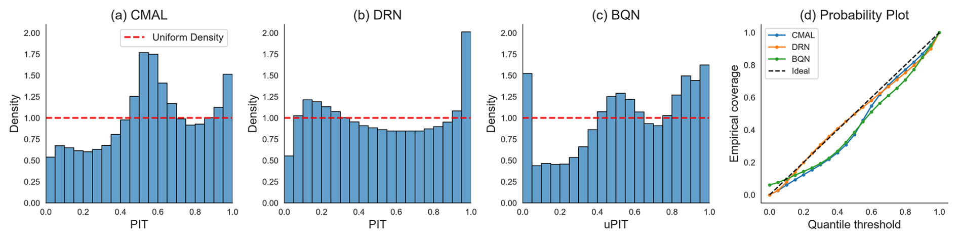
Figure F2 PIT histograms for the (a) CMAL, the (b) DRN and the (c) BQN. The x axes indicate the PIT values from the entire testing data ($\approx \mathrm{1.27}\times {\mathrm{10}}^{\mathrm{6}}$ values) binned into 20 equal-sized bins. The y axes give the density of these bins. The red dashed line indicates the ideal uniform distribution. Bins with density less than 1 imply that the model predicts a lesser number of these probability values than actually observed. Similarly, bins with density more than 1 indicate that the model assigns these probability values more frequently than actually observed.