Changes in groundwater-surface water interactions following two centuries of irrigation practices and groundwater use in the Upper Ganges-Yamuna interfluve, North India

The Indo-Gangetic Basin (IGB) is a global hotspot for groundwater overexploitation. Previous studies have shown that groundwater levels initially rose due to enhanced recharge following the construction of irrigation canals, but subsequently declined as agricultural, municipal, and industrial abstractions intensified. However, the relative impacts of separate recharge and abstraction components (precipitation, canal leakage infiltration, irrigation return flow, and irrigation, municipal and industrial abstraction), remain unclear, as do the effects on groundwater-surface water interactions and environmental flows. This study therefore aims to quantify spatio-temporal changes in groundwater recharge and abstraction components over the past two centuries and assesses how these changes have impacted groundwater–surface water interactions in the Upper Ganges–Yamuna interfluve in northern India.

Groundwater model simulations indicate that canal water infiltration following canal construction after 1830 increased groundwater recharge and groundwater discharge to local rivers. Although canals continue to provide significant recharge, rapid rise in groundwater abstraction since the 1970s has lowered groundwater tables and reduced groundwater discharge to surface waters. Currently irrigation accounts for roughly 85 % of the abstractions, with municipal (15 %) and industrial (< 1 %) uses accounting for much smaller shares. The model simulations indicate that around 2000 local rivers likely shifted from draining to infiltrating conditions. This change in groundwater–surface water exchange may affect environmental flows and increase the vulnerability of groundwater to contamination where surface waters are polluted. Although both the Yamuna and the Ganges show reduced groundwater exfiltration, they are not (yet) infiltrating.

1 Introduction

Groundwater is vital for humans and ecosystems but is increasingly threatened by excessive abstractions, particularly in semi-arid irrigated areas (de Graaf et al., 2017). Groundwater depletion is widely occurring within the Indo-Gangetic Basin (IGB) making it one of the worlds hotspots of groundwater overexploitation (Gleeson et al., 2012; Marinelli et al., 2024). Satellite data from the Gravity Recovery and Climate Experiment (GRACE) reveal a steady decline in total water storage across Northern India over the past two decades (Panda et al., 2021; Rodell et al., 2009). The GRACE records since 2002 (Rodell et al., 2009), which is relatively short considering that small-scale canal systems in the Indo-Gangetic Basin (IGB) date back to the 16th century under Mughal rule (Jain et al., 2022) and the development of modern irrigation canal systems began in the 19th century with the Eastern Yamuna irrigation canal in 1830 (Irrigation and Water Resources Department, 2026).

Long-term groundwater monitoring data offers a broader perspective. Analysis of observation wells in northwest India and central Pakistan (MacAllister et al., 2022) go back to 1900 and reveals a net increase in groundwater storage from 1900 to the 1970s. This is a result of groundwater recharge by leakage from irrigation canals, which is earlier defined as the largest and longest unintended anthropogenic recharge globally (MacAllister et al., 2022; Scanlon et al., 2023). Groundwater storage peaked in the 1970s. Between the 1970s and 2000, trends became spatially heterogeneous: while some areas continued to experience rising groundwater levels due to sustained canal leakage recharge, others began to show declines associated with increasing groundwater abstraction. Overall, groundwater level changes from 1900 to 2010 reflect the evolving interplay among canal construction, abstraction, and precipitation variability (MacAllister et al., 2022). However the magnitude and relative contributions of different recharge and abstraction components to the observed changes remain unclear. In particular, the roles of sector-specific abstractions (irrigation, domestic, and industrial use) and irrigation return flows in shaping groundwater dynamics are insufficiently constrained.

At the global level, Scanlon et al. (2023) have shown that groundwater recharge and abstractions not only affect groundwater table depth but also affects the interaction with surface water. de Graaf et al. (2019) showed how groundwater table changes may affect groundwater-surface water interactions that amongst others affects environmental river flows. Maheswaran et al. (2016), using a regional groundwater model, suggested that parts of the Ganges and Yamuna may have shifted from draining to infiltrating due to local abstractions. However, the evolution of these interactions since canal construction in the mid-19th century has been unknown. Local tributaries also play a key role (de Vries, 1995), yet their historical changes remain undocumented.

The surface water–groundwater (SW–GW) interactions are important to understand as it also highly impacts the surface water quality. Reduced baseflow limits pollutant dilution, while contaminated river water can infiltrate into aquifers (van Broekhoven et al., 2024), posing public health risks when groundwater is used as source for drinking water (Lewis, 2007).

Despite our understanding of long-term groundwater table trends, a deeper understanding of the historical and spatial evolution of groundwater balance components, including how water-use sectors and return flows developed over time, is crucial for improving predictions and designing effective management strategies to protect water resources, environmental flows, and community well-being. A better understanding of historical system behaviour is beneficial to set realistic restoration objectives (Forstner et al., 2025).

Long-term monitoring data are only available for the northwestern IGB (Punjab and Haryana). How groundwater table depth and SW–GW interactions have responded to variations in recharge and abstraction in the more humid eastern region, e.g. state of Uttar Pradesh, remains unknown. We focus on the Upper Ganges-Yamuna interfluve, which contains the Hindon River, as the water system in this region is heavily modified by human activity (van Broekhoven et al., 2024).

This study aims to quantify the spatio-temporal evolution of groundwater recharge and abstraction components, and their effects on groundwater tables and GW–SW interactions in the Upper Ganges–Yamuna interfluve of the IGB. First, the spatio-temporal evolution of groundwater recharge and abstraction components is reconstructed for the period from pre-canal conditions (< 1830) to recent times (2016). These recharge and abstraction estimates are subsequently used as uncertain external forcings in a spatially explicit, physically based groundwater model (MODFLOW 6). The model simulates groundwater heads, groundwater storage evolution, and SW–GW exchange fluxes. This analysis improves understanding on the contribution of different water use sectors to groundwater dynamics and provides a basis for sustainable groundwater management.

2 Study area and methods

2.1 The Upper Ganges-Yamuna interfluve

The Upper Ganges-Yamuna interfluve (Fig. 1) is part of the Ganges basin, covering roughly 16 500 km² and measuring up to 100 km wide and 220 km long. It is located in western Uttar Pradesh and southern Uttarakhand, India, situated north of Delhi. The Hindon River subbasin, located at the centre of the study area, is a rainfed tributary of the Yamuna that originates in the Shivalik Hills and is joined by its tributaries, Krishni and Kali Rivers (van Broekhoven et al., 2024). The region has a humid subtropical climate, with most rainfall occurring during the monsoon season (June–September), around 700–950 mm, while the non-monsoon period (October–May) receives only about 100–200 mm of rainfall (Mourad et al., 2024).

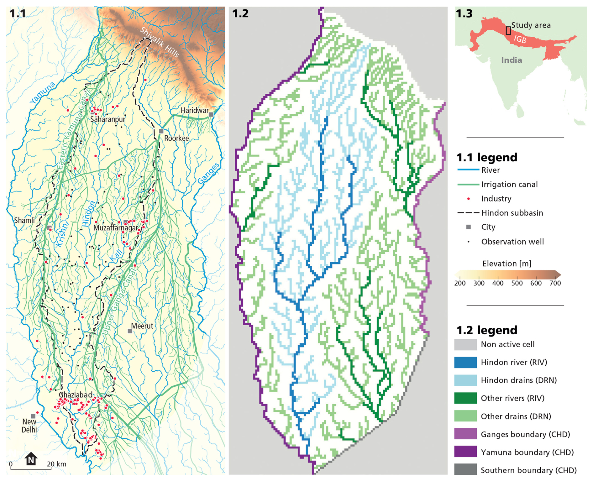
Figure 1 (1.1) Study area with rivers, irrigation canals and surface elevation (HydroSHEDS, Lehner et al., 2008). (1.2) MODFLOW model schematisation of rivers and boundaries (MODFLOW package names shown in brackets). (1.3) Location of study area within the Indo-Gangetic Basin (IGB). IGB outline is adapted from Bonsor et al. (2017).

Hydrogeologically, the subbasin is part of the Indo-Gangetic alluvial aquifer system, comprising thick sequences (up to more than 200 m) of medium- to coarse-grained oxidised sands with high hydraulic conductivity (30–50 m d⁻¹) that can be largely considered as a single aquifer (Bonsor et al., 2017). Depths of groundwater table typically range from a few meters up to more than 30 m, with deeper water tables occurring in coarse alluvial deposits along the basin's northern margin (Alam and Umar, 2013; Bonsor et al., 2017; Umar et al., 2008; van Dijk et al., 2020). A regional north-to-south gradient of approximately 0.55 m km⁻¹ characterises the flat topography (van Broekhoven et al., 2024).

Groundwater extraction has increased substantially since the mid-20th century due to agricultural intensification and urban expansion. While early irrigation primarily relied on canal networks, such as the Upper Ganga Canal built in 1854 (Drew, 2014) and the Eastern Yamuna Canal constructed in 1830 (Irrigation and Water Resources Department, 2026), the post-Green Revolution period marked a shift toward intensive groundwater use (Pingali, 2012). This transition was driven by technological advancements, including the adoption of hand pumps, diesel pumps and electric pumps, as well as policy incentives promoting groundwater use, such as the provision of free electricity for irrigation (Panda et al., 2021). As a result, groundwater tables dropped (Jadav and Yadav, 2025; Mendoza et al., 2026). This has contributed to the reduced flow of the Hindon River outside the monsoon season, particularly in its headwaters, which are now ephemeral (van Broekhoven et al., 2024). As groundwater tables continue to fall, sections of the river may have shifted from draining to infiltrating from the river into the surrounding aquifer (van Broekhoven et al., 2024). Water pollution sources include industrial discharges (e.g., paper and sugar manufacturing), municipal wastewater in rivers (Lewis, 2007) and ponds (van Broekhoven et al, 2024), and agricultural pollution from fertilizers and pesticides (Gautam et al., 2022).

2.2 MODFLOW 6 – model schematisation

The complex interplay between recharge, abstractions, groundwater table depth, and groundwater–surface water interaction was modelled using MODFLOW 6 (Langevin et al., 2017). This spatially explicit, process-based model incorporates the spatial and temporal distribution of recharge and abstraction components. These processes are the primary drivers of groundwater balance change. However, quantifying these components and subsurface properties requires assumptions, introducing uncertainties. To address this, multiple model realisations with different parameter values for subsurface properties and recharge and abstraction inputs were used to generate a wide range of realisations. Unrealistic realisations were filtered out, resulting in narrower parameter ranges.

This study used a transient MODFLOW 6 model with a regular grid consisting of a single layer, 231 rows, and 108 columns, with 1000 m × 1000 m cells. The model was set up and analysed using the Flopy Python package (Bakker et al., 2016). A high spatial resolution was selected due to the observed variability in recent groundwater trends (Joshi et al., 2021; van Dijk et al., 2020) and findings by van Broekhoven et al. (2024), which indicate that recharge components such as canal leakage have highly localised influences (< 1 km) based on groundwater quality signatures. The simulation period spans over two centuries, covering pre-canal development to the present, (1800–2016) in yearly time steps, focusing on long-term trends rather than seasonal dynamics.

The aquifer was represented as a single hydrogeological unit using one model layer, due to discontinuous and local clay layers (Bonsor et al., 2017). This is consistent with the schematisation of Maheswaran et al. (2016), who applied a uniform aquifer thickness of 200 m. The model top elevation was derived by resampling the mean elevation from the HydroSHEDS Digital Elevation Model (DEM) (Lehner et al., 2008).

Model boundaries were defined to reflect natural hydrogeological system limits where possible. The eastern and western boundaries are defined by the Ganges and Yamuna rivers and were simulated as Constant Head Boundaries, assuming groundwater head equal river levels due to their size and strong hydraulic connection. Because a yearly time step was applied, seasonal variability was not included. Furthermore, the use of Constant Head boundaries implies that interannual variability in average river stages is assumed to be limited. The northern boundary is defined by the Shivalik Hills and treated as a no-flow boundary. Along the southern boundary, where no clear natural border exists, a constant head boundary was set sufficiently far (> 10 km) from the Hindon subbasin to minimise edge effects.

The Hindon River and its main tributaries are simulated by the RIV package, allowing for both infiltration and exfiltration, as the river is effluent-fed and flows year-round, with indications of ongoing infiltration (van Broekhoven et al., 2024). Smaller streams and drains, which typically dry up outside the monsoon season, were simulated using the DRN package, permitting only discharge. Water levels for rivers, drains, and constant head boundaries (including the Ganges and Yamuna rivers) were set equal to the resampled minimum elevation value from the HydroSHEDS DEM (Lehner et al., 2008). Irrigation canals were represented as recharge (RCH package) rather than explicit surface-water boundary conditions (e.g., RIV package). This treats canal leakage as disconnected surface water recharge, independent of simulated groundwater levels, reflecting their typical elevated position relative to deeper groundwater tables, which ensures predominantly downward leakage to the aquifer. Canal-derived recharge comprises two components: (i) direct leakage from the mapped canal network and (ii) indirect recharge through irrigation return flow. The latter accounts for both canal water and groundwater used for irrigation, with their spatially varying contributions derived from census data (Sects. A5 and A6).

The model focuses on the spatial and temporal variation of recharge and abstractions. Recharge components include rainfall, canal water leakage, irrigation return flow, and municipal return flow. Sectoral water withdrawals include irrigation, municipal, and industrial uses. These model forcings (recharge and abstraction) generate outputs such as groundwater table depths and fluxes across boundaries, rivers, and drains. Figure 2 illustrates the groundwater balance components, with black arrows representing model inputs and blue arrows indicating model outputs.

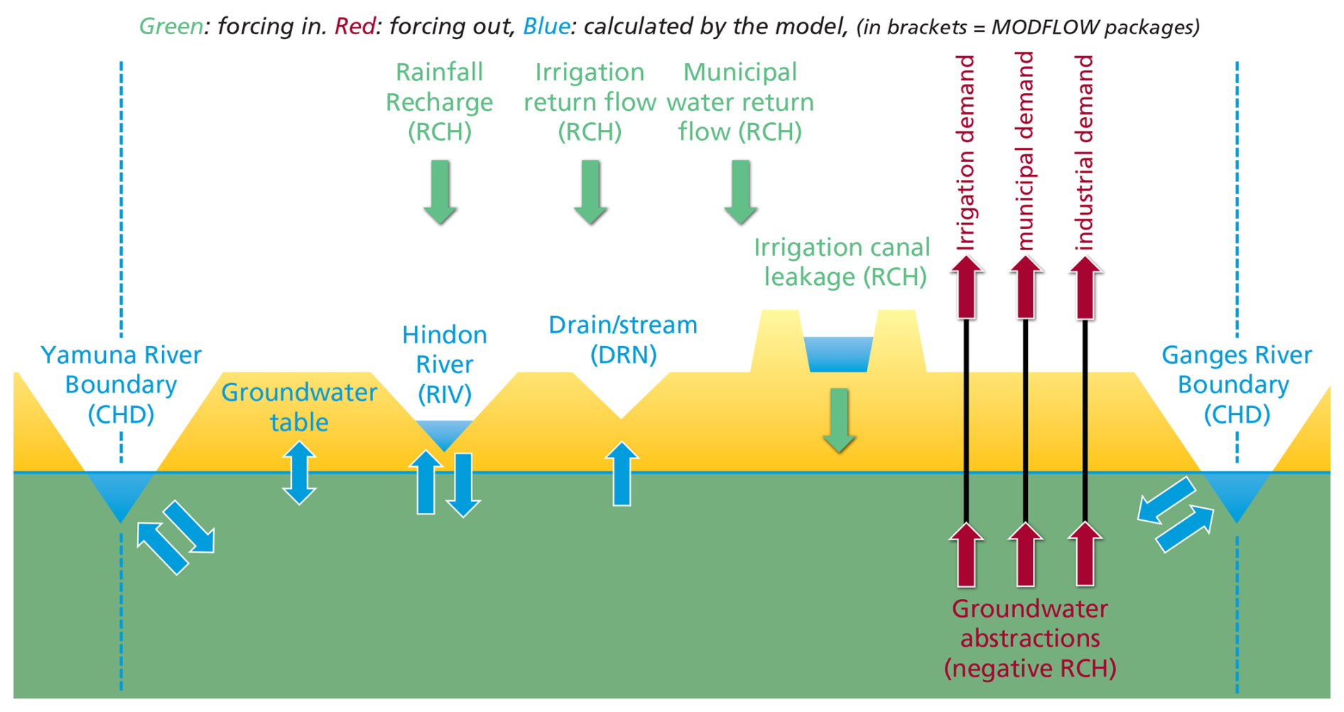
Figure 2 Conceptual representation of groundwater balance components in the model domain. Green arrows indicate model input fluxes (forcing) representing recharge sources, while red arrows indicate model input fluxes (forcing) representing groundwater abstractions (simulated as negative recharge). Blue arrows represent fluxes simulated by the model (i.e., model outputs), including groundwater–surface water exchanges and boundary flows (MODFLOW package names shown in brackets).

Spatio-temporal information was required for each recharge and abstraction component over the simulation period. As such datasets are not readily available, multiple data sources were integrated and informed assumptions were applied to derive spatially and temporally consistent estimates for each component. In general, available spatially explicit data were used for the current situation, while historical data were collected to establish trendlines to hindcast past conditions. The aim was to capture overall temporal trends in a spatially distributed manner rather than precise estimates for each cell and time step. The construction of spatio-temporal datasets for all recharge and abstraction components per model cell and time step is described in Appendix A.

2.3 Monte Carlo analysis

We used the Monte Carlo method to account for uncertainty in input data (e.g. Ballio and Guadagnini, 2004; Bekesi and McConchie, 1999; Kahe et al., 2021). Table 1 shows the prior parameter ranges for hydraulic conductivity, aquifer thickness, and specific yield derived from the literature. To maximise realisations variability, we assumed uniform probability distributions for these parameter ranges. River and drain conductivity had log-uniform probability distribution (Table 1).

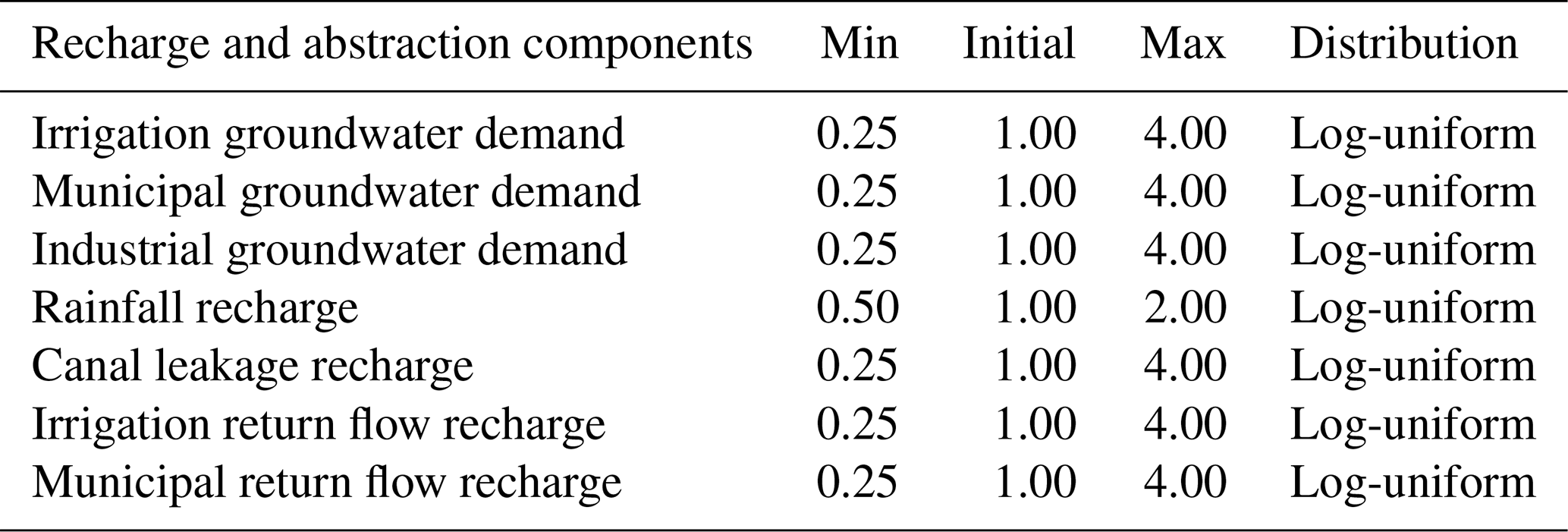
For computational efficiency, we combined all recharge and abstraction components into a net recharge variable, calculated as the sum of all recharge minus abstractions components. Since the model uses a single layer, abstractions could be treated as negative recharge. We applied uniform uncertainty factors between 0.25 and 4 to each component, except for rainfall recharge where we considered between 0.5 and 2 more realistic (see Table 2). This preserves temporal trends and spatial variations per component, but for the cumulative net recharge, this yields temporally and spatially varied values across realisation runs. Log-uniform probability distributions were used for each multiplication factor to get a uniform distribution of factors bigger and smaller than the initial estimate.

Table 1 Bandwidth of prior aquifer properties parameters.

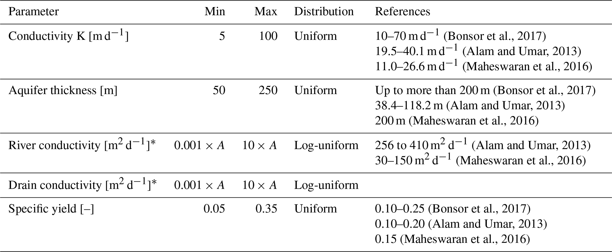
^* The river and drain conductivity is calculated by the surface water area per cell (A) multiplied by the vertical leakage coefficient (which is the riverbed conductivity divided by riverbed thickness and has unit d⁻¹). The surface water area per cell (A) varies for each model cell from 151 to 10 960 m² for river cells and from 2.6 to 22 425 m² for drain cells.

Table 2 Multiplication factors for recharge and abstraction components (prior parameter ranges), log-uniform distribution.

The model executed 1500 simulation runs, each with randomly sampled aquifer properties, and net recharge derived from the separate recharge and abstraction components with random multiplication factors. To stabilise initial conditions, each run had a 100-year warm-up period.

All model realisations were evaluated against observational data and subjected to constraints to ensure realistic outcomes, a process considered rejection sampling. Regarding observational data, groundwater level data from 94 observation wells (containing data between 1990–2018) with at least 10 years of monitoring data were used for evaluation. Data were provided by the Ground Water Department, Uttar Pradesh, and the Central Ground Water Board, Ministry of Jal Shakti. Data availability varied in space and time, some wells were recorded 4 times a year, while others were measured incidentally. We used the Mean Absolute Error (MAE) as a measure of goodness of fit and the Mean Error as a measure of bias. Both objective functions are robust against outliers as they do not use squared values and are easily interpretable as both measures have the same units as the observations. We accepted all model realisations with Mean Absolute Error (MAE) ≤ 7.5 m and Mean Error (bias) between −5 and +5 m.

To ensure physically plausible system behaviour beyond the observation period, model runs were screened using four realism criteria: (i) when simulated groundwater tables exceeded ground level in more than 2.5 % of active cells, since extensive wetlands or persistent surface waterlogging are not reported for the study area; (ii) when more than 5 % of active cells showed groundwater depths greater than 50 m below ground level, since across most of the study area groundwater is widely used and easily accessible and thus shallower; (iii) the simulated yearly average baseflow of the Hindon River for the period 1997–1999 must not exceed 65 m³ s⁻¹. This threshold represents the mean observed discharge (65 m³ s⁻¹) measured at Mohannagar between April 1997 and March 1999 (Jain and Sharma, 2006) and limits unrealistically high groundwater contributions to river discharge (> 100 %); (iv) under natural (pre-canal: < 1800) conditions, the simulated yearly average baseflow in the Hindon River subbasin was required to remain positive (> 0 m³ s⁻¹), reflecting expected groundwater exfiltration to the river in the absence of major anthropogenic alterations. Only runs that performed adequately against observations and realism checks were retained.

3 Results

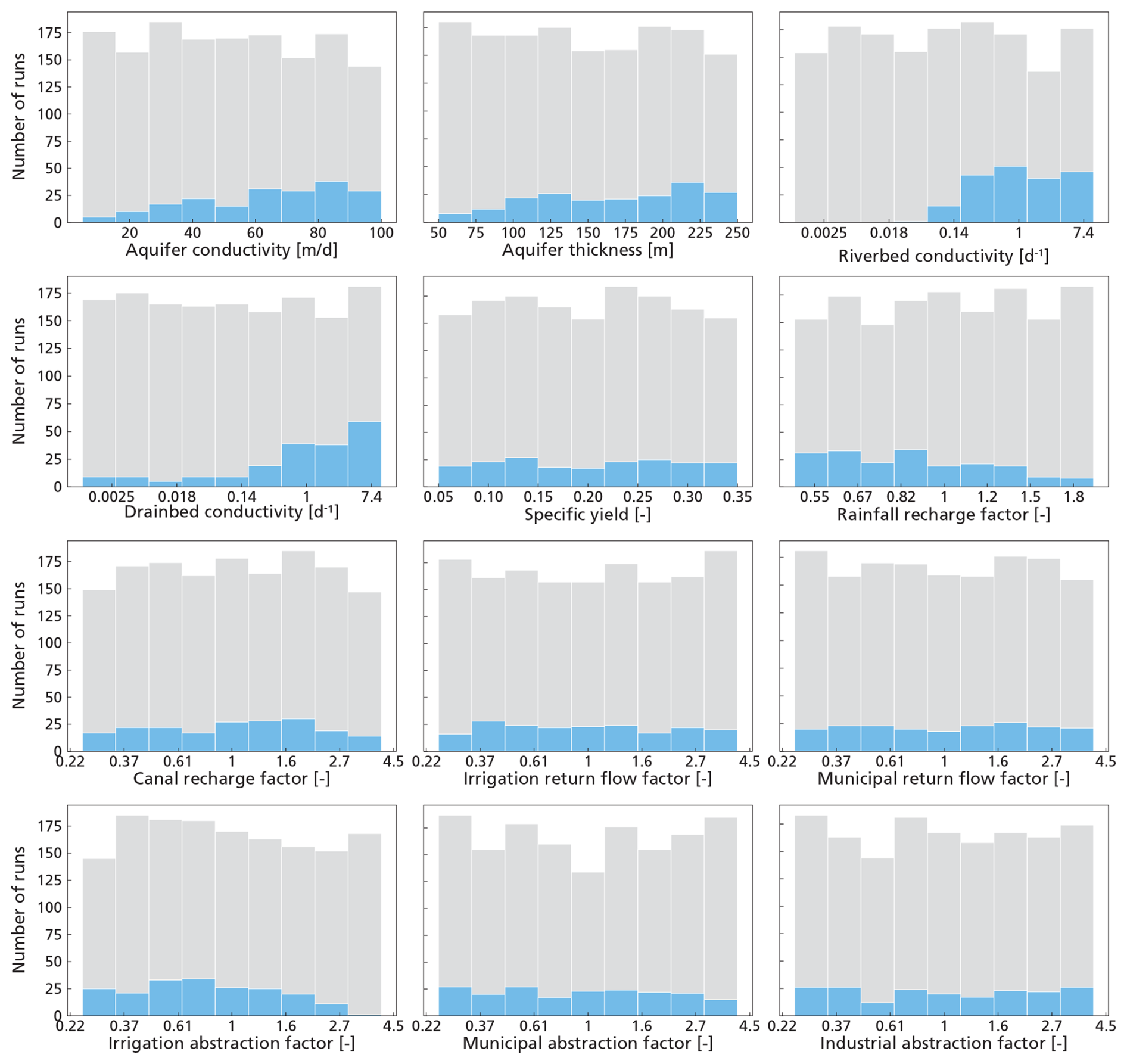
From the 1500 model realisation runs, 198 runs (13 %) were unsuccessful due to numerical instability. Among the remaining 1302 runs, 196 (15 %) met all performance and realism criteria. Among these 1302 runs, 39 % failed due to MAE > 7.5 m, 18 % due to mean error > 5 m, 24 % due to mean error < −5 m, 79 % due to groundwater exceeding ground level, 5 % due to excessive groundwater table depth (> 50 m), 2.2 % due to unrealistic high Hindon baseflow (1997–1999), and 1.8 % due to negative pre-canal baseflow. The simulated groundwater heads generally agree reasonably well with observations (R²=0.86), with no systematic bias, although some individual differences exceed 10 m. The model broadly captures observed declining trends, but tends to underestimate stronger declines and smooth out local variations. A more detailed evaluation of model performance against observed groundwater heads and trends is provided in Appendix B. Appendix B also presents observed groundwater heads together with the simulated posterior ensemble (minimum, median, and maximum) for the 12 wells with the longest observation records. Figure 3 presents histograms of the parameter distributions for the prior ensemble and posterior ensemble (the 196 realisations that met all criteria). Comparison of the posterior ensemble with the full ensemble shows that the posterior ensemble generally have higher aquifer conductivity and thickness and also higher river bed and drain bed conductivity. Additionally model performance was further influenced by recharge and abstraction factors. Rainfall recharge factors greater than 1 resulted in more rejected realisations, as did irrigation demand factors exceeding 1.5.

Figure 3 Parameter distribution priors (grey) and the posterior ensemble (blue).

3.1 Dynamics in recharge and abstraction components

Figure 4 illustrates the initial estimates of recharge and abstraction components since 1800, revealing distinct shifts in groundwater usage. Only after 1900 there was information on annual precipitation variability by CRU TS. Up to 1830, the system was dominated by natural rainfall recharge, which formed the primary input to the groundwater system. With the construction of the irrigation canal network since 1830, recharge volumes increased, augmenting the overall groundwater balance. However, from the 1970s onward, a pronounced rise in groundwater abstractions marked a transition toward increasing anthropogenic pressure directly on groundwater. This trend intensified between 1980 until 2010. The groundwater abstraction rates increase seem to flatten in the last decade. Currently, the primary recharge components are rainfall (approx. 50 %–80 %) and irrigation return flow (approx. 10 %–25 %), followed by canal leakage (approx. 10 %), with municipal water return flow contributing to a minor extent (approx. 2.5 %). Conversely, irrigation remains the dominant component of groundwater abstraction (approx. 80 %–85 %), with municipal (approx. 10 %–20 %) and industrial (< 1 %) uses accounting for smaller, though locally sometimes significant, proportions.

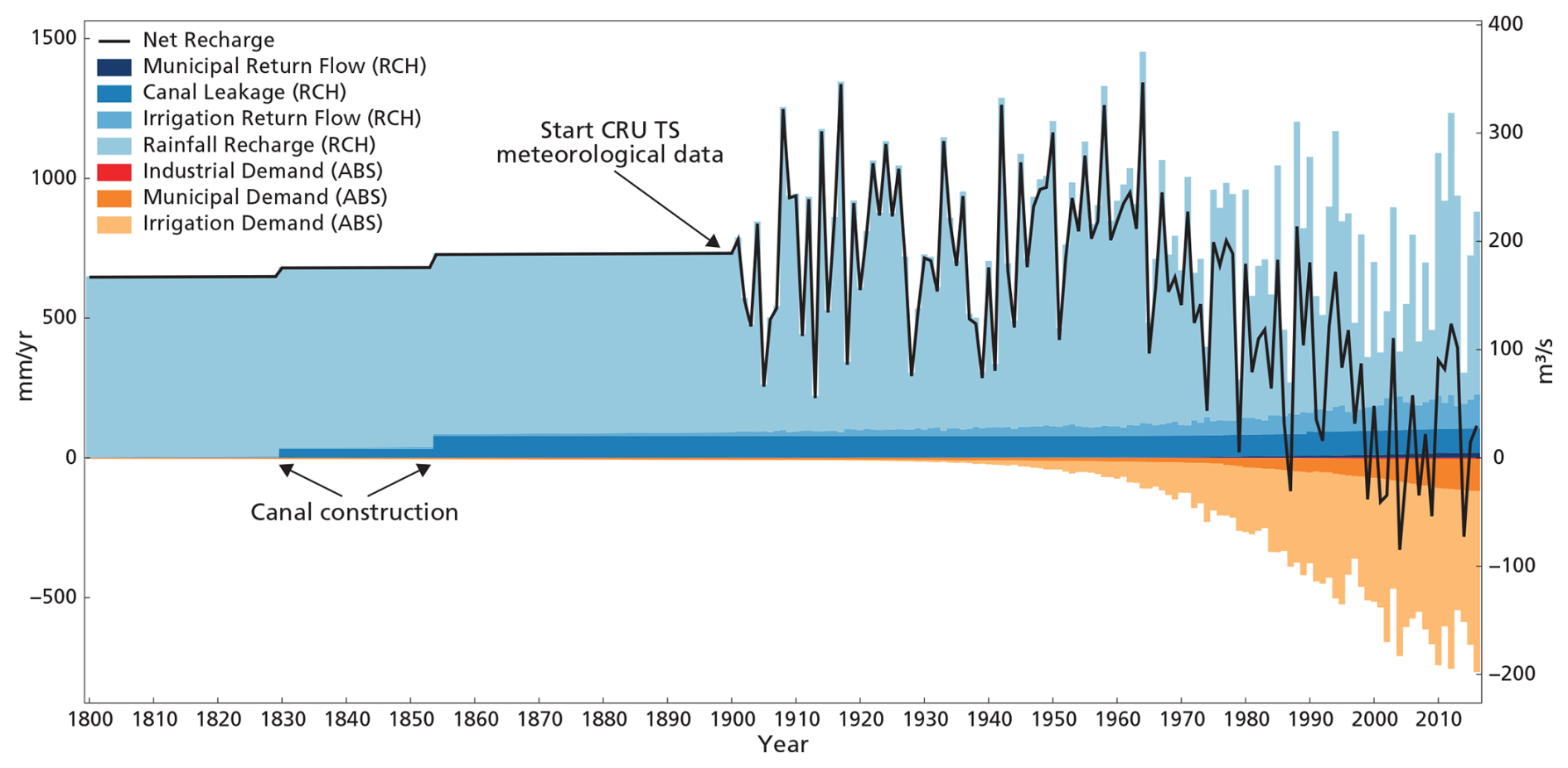
Figure 4 Initial estimates of changes in recharge (+) and abstractions (−) components (black line = net recharge, which is sum of all recharge minus all abstractions components).

The black line in Fig. 4 represents the net recharge, which is up to 1940 equal to the rainfall recharge, and is calculated as the sum of all recharge components minus all abstractions. A negative net recharge indicates that, on an annual basis, more groundwater is abstracted than recharged. Figure 5 illustrates the bandwidth of net recharge for the posterior ensemble. Net recharge first increased by canal recharge, but within the uncertainty bands in 1970 and on average around 2000, the system has been characterised by also negative net recharge. Uncertainty ranges are higher after 2000, due to the multiple components that become relevant for the net recharge.

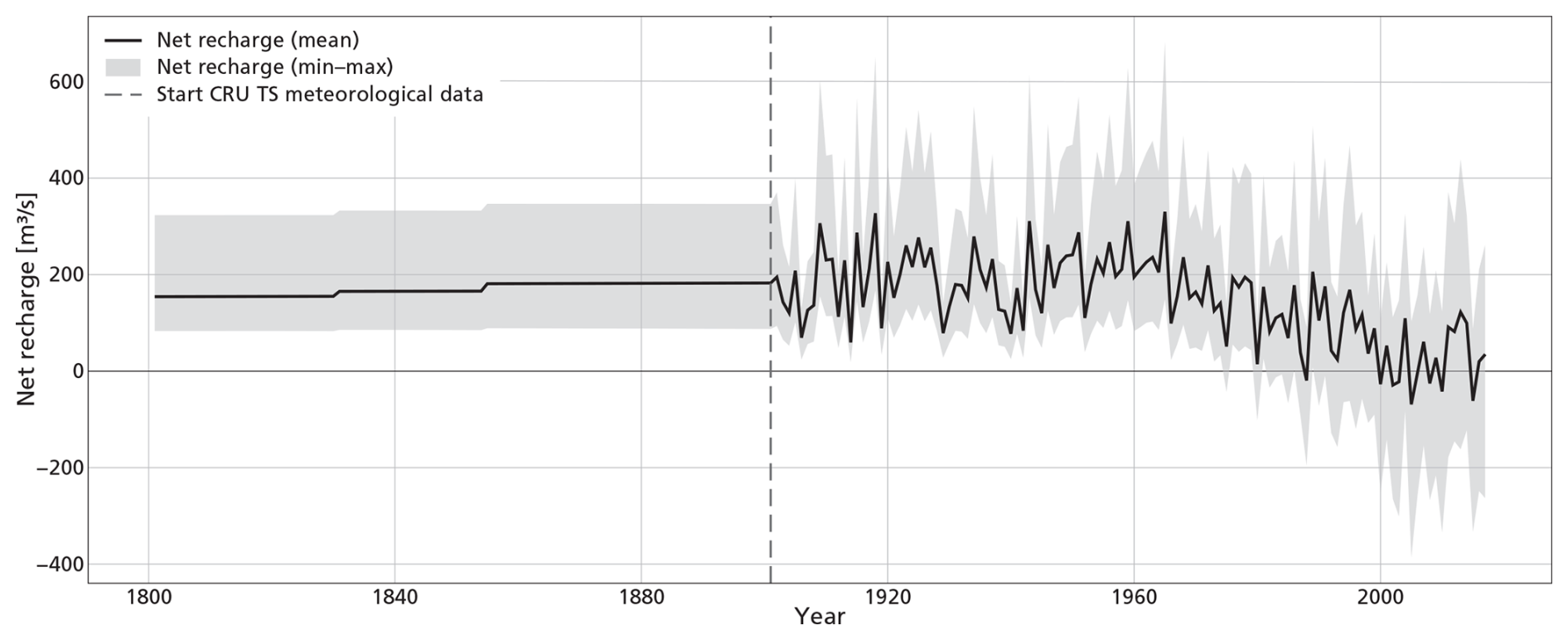
Figure 5 Net recharge input of the posterior ensemble (min, mean, max). Net recharge is calculated as the sum of all recharge (+) minus all abstractions (−) components.

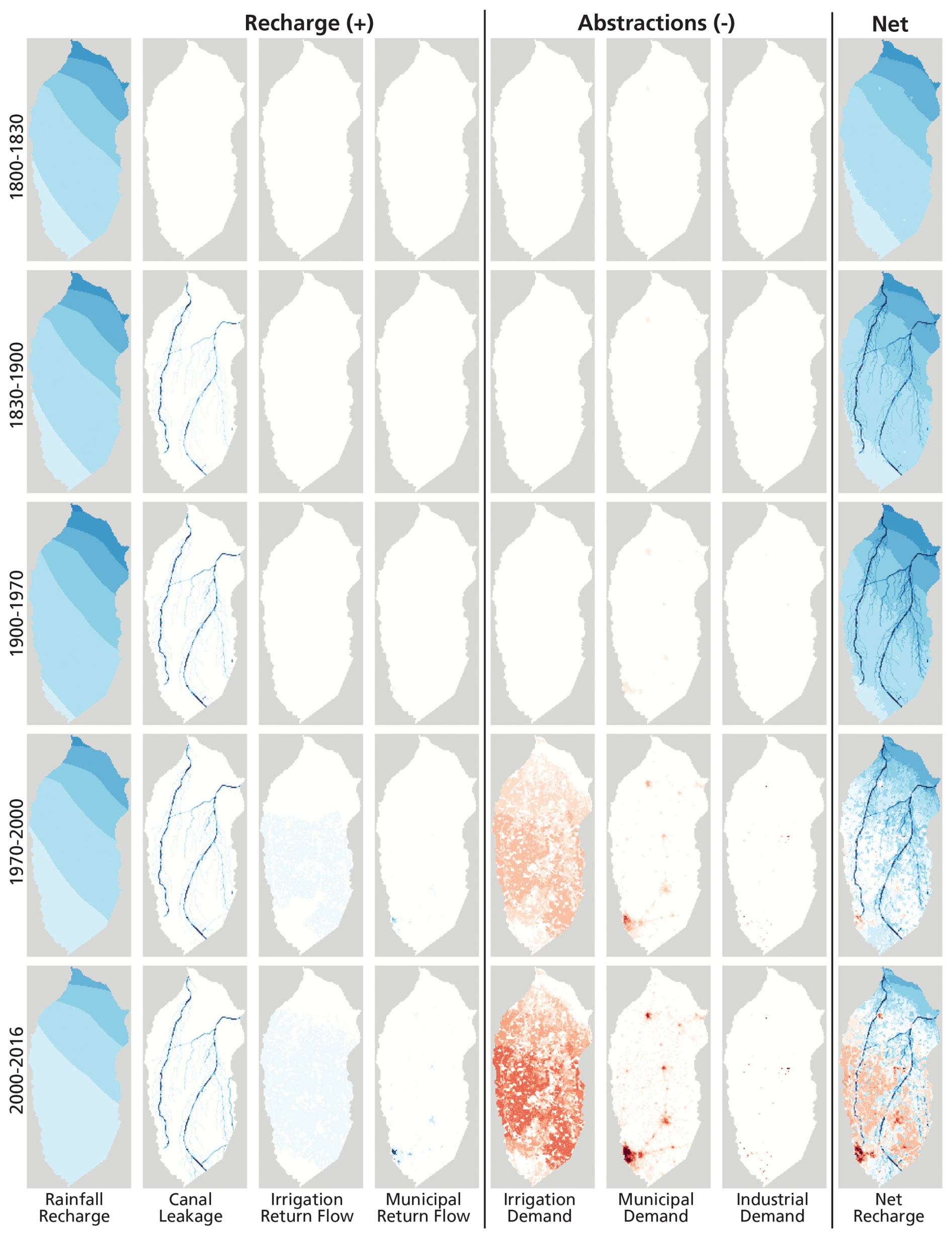
Figure 6 Spatial variation of initial estimates of recharge (+) and abstractions (−) components during time periods.

Figure 6 shows the spatial variation of recharge (+) and abstraction (−) components averaged over several time periods. Rainfall recharge exhibits the highest rates along the Shivalik Hills (northeast) and gradually decreases towards the southwest. Also a decrease in time is observed, although the declining gradient from northeast to southwest stays constant. Canal leakage is concentrated along the main canal network and is lower along secondary branches. Over time, newly developed canal areas become visible, although their extent remains relatively small compared to the main irrigation network. Irrigation return flow (recharge) and irrigation demand (abstraction) are distributed fairly evenly across the region, except in the north along the Shivalik Hills and in the south around urban settlements such as Ghaziabad, where there is limited irrigation. Municipal return flow and municipal demand are highly localised around major towns, with clear hotspots at Ghaziabad, Meerut, Muzaffarnagar and Saharanpur. Industrial demand is also associated with municipal areas but is more sparsely distributed. Net recharge remains predominantly positive until 2000. During the period 1970–2000, negative net recharge (i.e., abstractions exceeding recharge) is mainly limited to areas around Ghaziabad. After 2000, large parts of the region exhibit negative net recharge, with a broad north–south division emerging around the latitude of Muzaffarnagar, separating predominantly positive conditions in the north from negative conditions in the south.

3.2 Effects on groundwater table

Figure 7 depicts groundwater table trends based on spatial median values. We used the mean of spatial medians per time step and model run to avoid bias toward deeper tables caused by the deep groundwater table in the Shivalik Hills. Groundwater table trends are closely aligned with those of net recharge. Following the construction of canals since 1830, median groundwater tables rose by approximately 0.5 to 1.0 m over the entire study area. From 1900 to 1970, groundwater tables increased slightly but generally remained stable. The annual variability is also depicted since 1900. However, since the 1970s, a marked and accelerating decline in groundwater tables has been observed. From around 2000 onwards, the rate of decline became less pronounced. By 2016, the median groundwater table depth had increased to an average of 10 m, compared to approximately 7.5–8.0 m in the pre-1830 “natural situation”.

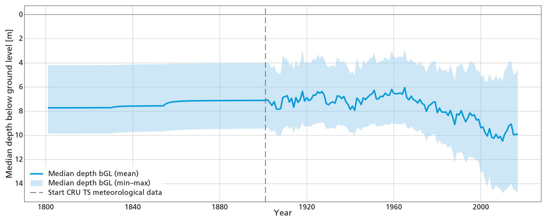
Figure 7 Median depth of groundwater table per time step, showing the ensemble minimum, mean and maximum of the posterior ensemble realisations.

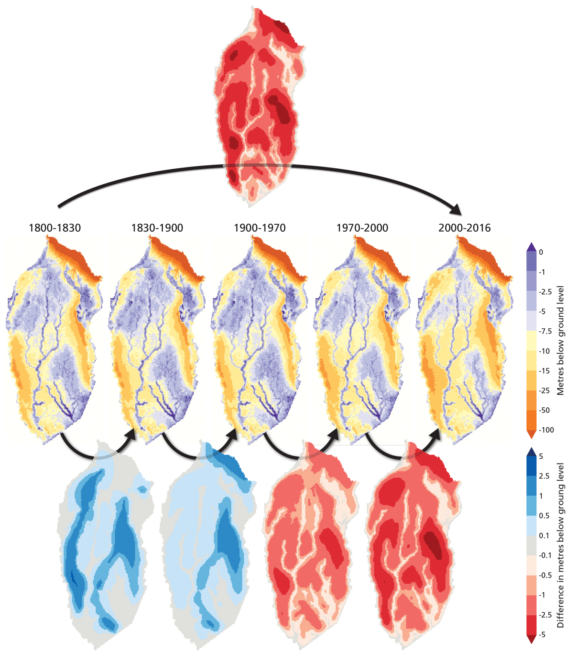
Figure 8 Mean depth of groundwater tables below ground level per period of the posterior ensemble realisations (middle panels, period mean) and difference between time periods (bottom). The difference maps show the mean of the period minus the mean of the previous period. The top panel shows the difference between the last period (2000–2016) and the first period (1800–1830).

Figure 8 shows spatial maps of depth of groundwater tables during several periods, together with maps showing the differences between a period and the previous period. It also shows the difference between the current period (2000–2016) and the “natural situation” (1800–1830). Overall, groundwater table is deeper in the Shivalik Hills, in the area between the lower reaches of the Yamuna River and the Hindon River, and along the left bank of the Ganges River. These areas coincide with higher ground elevations. The regional groundwater gradient generally follows a north–south direction. The first difference map indicates increasing groundwater tables, mainly around the irrigation canals. The second period (1830–1900 versus 1900–1970) reflects relatively high rainfall recharge in the Shivalik Hills during 1900–1970. Since the 1970s, groundwater table declines are visible across most of the study area. Near the rivers, declines are negligible, whereas areas farther from the rivers show the most pronounced groundwater table declines. After 2000, the mean groundwater tables (2000–2016) declined again compared to the previous period (1970–2000).

3.3 Effects on groundwater – surface water interactions

Figure 9 shows the temporal variation in groundwater exfiltration fluxes to river surface water on the Upper Ganges–Yamuna interfluve (Hindon River and other local rivers), and to the adjacent reaches of the Ganges River and Yamuna River. Exfiltration refers to groundwater drainage and discharge from the aquifer to surface water bodies. A positive exfiltration flux indicates groundwater flow to the river, whereas a negative flux indicates infiltration of river water into the aquifer. During the pre-groundwater-exploration period (before the 1970s), Hindon River and other local rivers, captured the majority of groundwater seepage, while only a smaller fraction discharged directly into the main channels of the Ganges and Yamuna. Groundwater outflow along the southern gradient is neglectable and thus excluded from the figure.

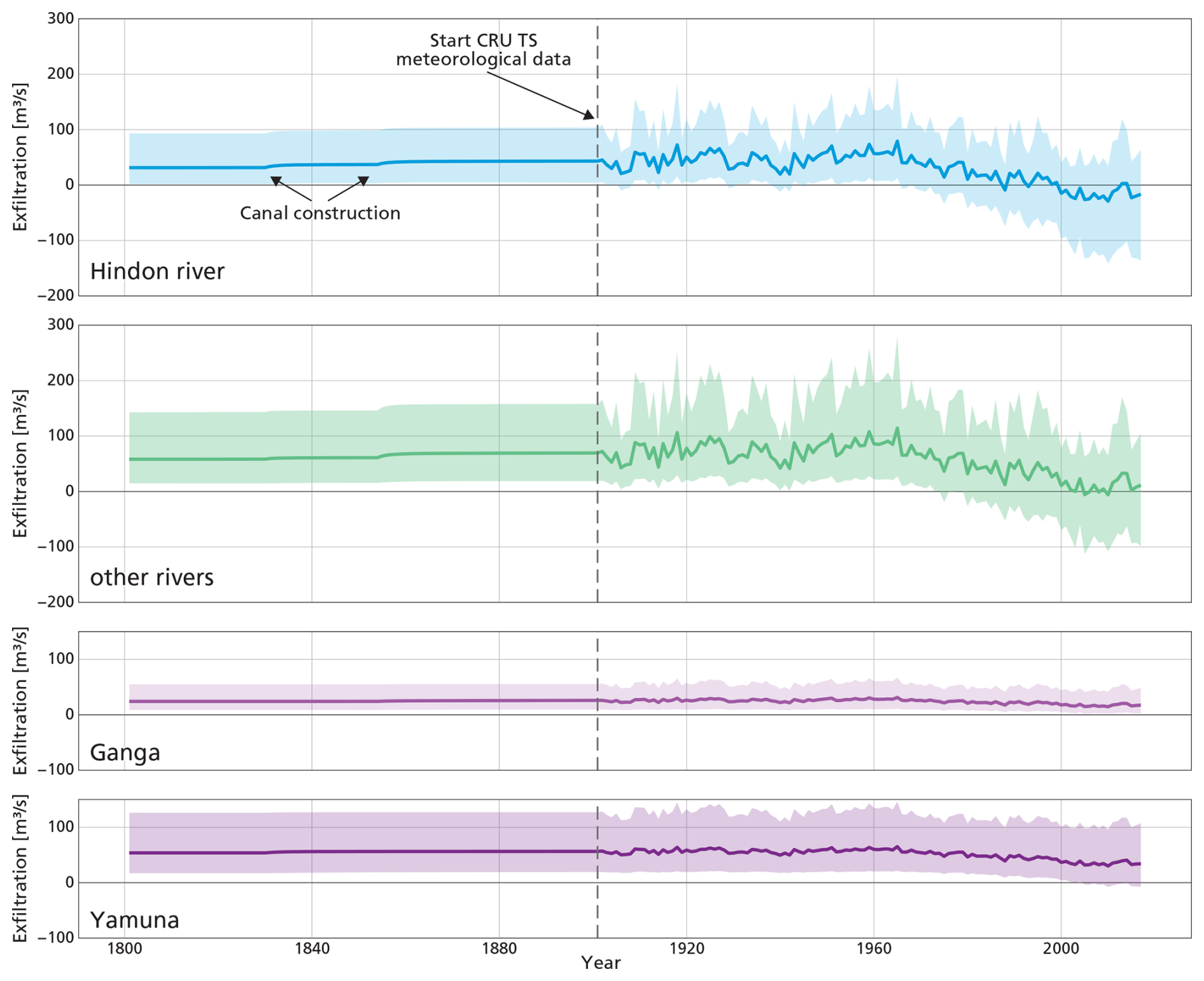
Figure 9 Exfiltration fluxes of groundwater to river surface water of the posterior ensemble (min, mean, max) of the Hindon River, other local rivers on the interfluve and the adjacent reaches of the Ganges and Yamuna rivers. A positive exfiltration flux indicates groundwater flow to the river, whereas a negative flux indicates infiltration of river water into the aquifer.

The trends in groundwater exfiltration fluxes closely follow those of net recharge and groundwater table depth. The construction of irrigation canals introduced additional recharge, which in turn increased groundwater exfiltration. Since the 1970s, however, groundwater exploration has led to a decline in exfiltration. This reduction is particularly pronounced in the Hindon River network, where most model runs indicate a shift from exfiltration to infiltration since around 2000. This implies the river on average now infiltrates more water year-round than it receives from groundwater. While some model runs suggest this switch began as early as the 1970s, others do not show a switch at all. Groundwater exfiltration to the adjacent reaches of the Ganges and Yamuna rivers has also declined, but nearly all model runs still indicate net exfiltration.

Figure 10 presents the spatial variation of surface water–groundwater interactions averaged over different time periods. The results predominantly show exfiltrating reaches for the “natural situation”, interspersed with several infiltrating reaches. Although groundwater table declines are spatially most pronounced near the canal network, changes in surface water–groundwater exchange are more widespread, with many river reaches showing increased infiltration or reduced exfiltration, after the construction of the irrigation canals. Similar patterns are observed in subsequent periods, with conditions largely reversing after the 1970s. Since around 2000, most of the Hindon River has shifted to an infiltrating state, whereas the sections near the Shivalik Hills foothills continue to be mainly exfiltrating.

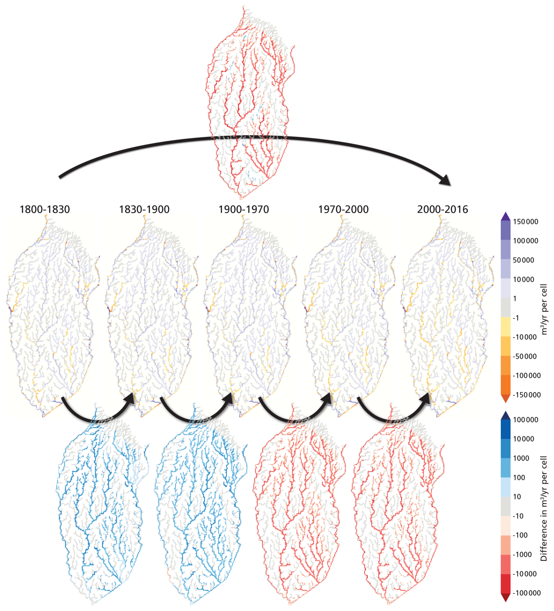
Figure 10 Spatial variation of of mean groundwater–surface water interaction per period of the posterior ensemble realisations (middle panels), expressed as exfiltration (+) and infiltration (−), and the differences between time periods (bottom panels). The difference maps show the mean of the period minus the mean of the previous period. The top panel shows the difference between the last period (2000–2016) and the first period (1800–1830).

4 Discussion

4.1 Groundwater balance evolution over the past two centuries in the Upper Ganges-Yamuna interfluve

Changes in groundwater recharge or abstraction influence groundwater levels with a temporal delay, as the system adjusts to shifts in storage. In our model, these delays emerge from groundwater system response, governed by storage, aquifer properties, and flow dynamics, rather than being prescribed separately. For instance, canal construction causes an immediate recharge increase, but water tables only rise gradually as water is stored and redistributed, while groundwater–surface water exchange fluxes also adjusts with delay following due to evolving hydraulic gradients. This, in turn, alters groundwater-surface water (GW-SW) interactions until a new equilibrium is reached (de Graaf et al., 2019; Bierkens and Wada, 2019; Scanlon et al., 2023). In practice, increased or decreased recharge leads over time to a new stable state with correspondingly higher or lower groundwater tables and exfiltration rate to rivers.

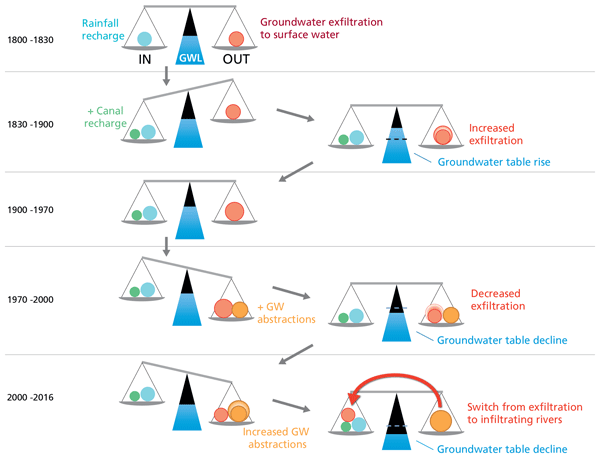
Figure 11 schematises how the groundwater balance in the Upper Ganges-Yamuna interfluve has evolved over the past two centuries. We identify five distinct time slices characterising this evolution:

1. Natural situation (1800–1830). A near-natural state where recharge is dominated by rainfall, the system is in balance, and groundwater tables are stable. Groundwater exfiltration to surface water more or less equals rainfall recharge.

2. Canal development (1830–1900). Canals enhance recharge, raising groundwater tables and increasing exfiltration. Our groundwater model illustrates this dynamic response following canal construction in 1830 (Eastern Yamuna Canal) and 1854 (Upper Ganga Canal). The system adjusts to the increased recharge, reaching a new equilibrium with elevated but stable groundwater tables and exfiltration rates.

3. Stable period (1900–1970). Long-term recharge is in equilibrium with long-term groundwater tables and exfiltration. Annual meteorological variability causes temporary fluctuations, with lower groundwater tables and exfiltration during dry periods and reversed during wet periods.

4. Groundwater development since Green Revolution (1970–2000). Increased irrigation demand is met by groundwater abstraction, reducing net recharge (recharge minus abstractions). This decline in recharge lowers groundwater tables and exfiltration rates.

5. Current period with intensive groundwater use (2000–2016). Groundwater abstractions exceed recharge, resulting in negative net recharge, rapidly declining groundwater tables, and a shift from draining to infiltrating local rivers.

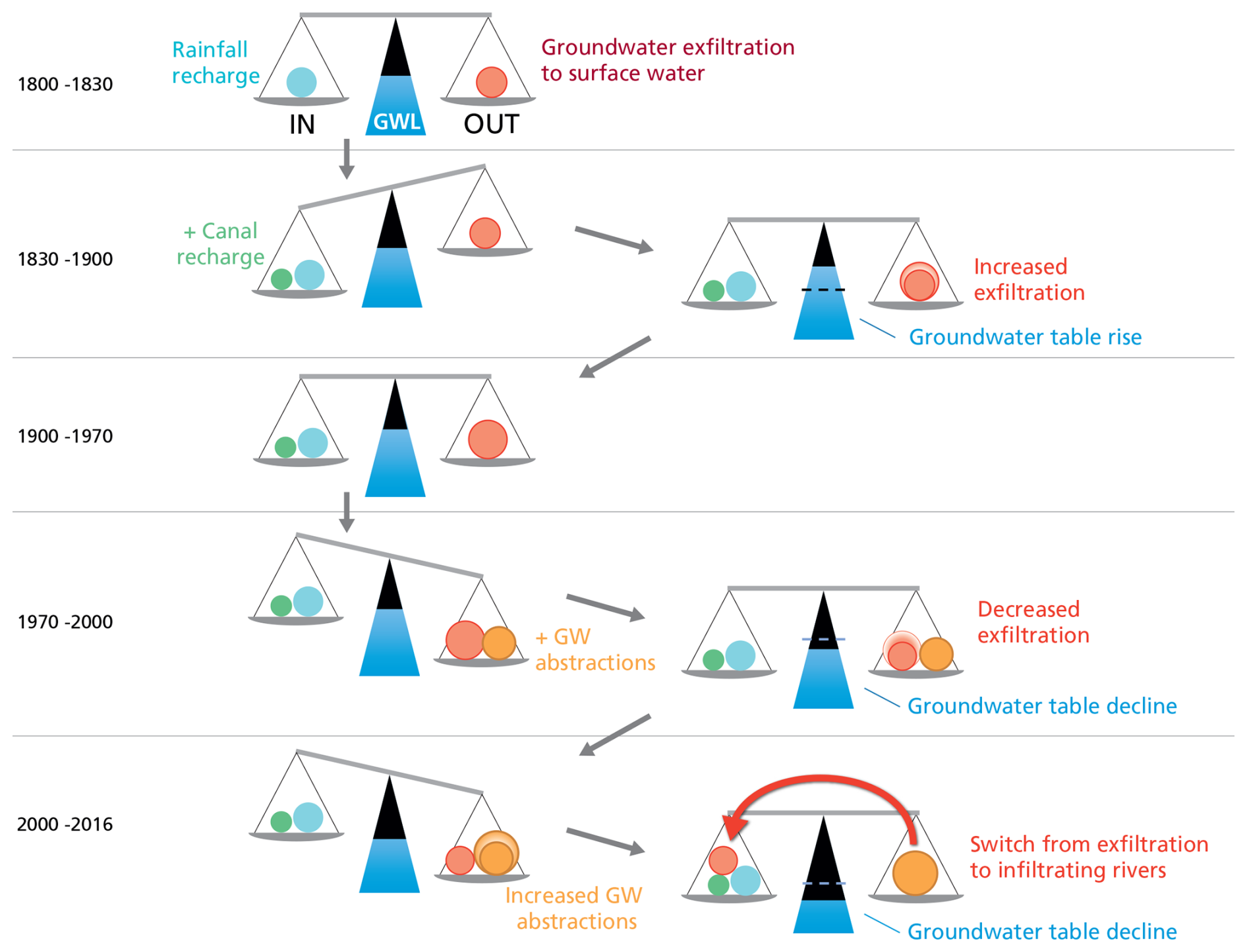
Figure 11 Changes in groundwater (GW) balance in the Upper Ganges–Yamuna interfluve from 1800 to present, based on the balance framework of Scanlon et al. (2023). The left panel shows system instability caused by changes in GW recharge or abstractions, while the right panel shows the system after adjustment to a new equilibrium, with altered groundwater tables and groundwater–surface water interactions.

The observed groundwater level rise from canal recharge aligns with MacAllister et al. (2022), though our study area shows smaller increases of 0.5–1 m on average (max 5 m) compared to their findings of several meters and up to 20 m in some locations. This discrepancy may stem from our area's wetter climate (located further east), different canal density or stronger surface water interaction, which limits storage changes. Additionally, a major difference is that the groundwater tables at our study area are currently below natural conditions (< 1830), whereas MacAllister et al. (2022) found current groundwater levels exceed those of a century ago. Panda et al. (2021) reported a groundwater storage decline equivalent to approximately 1 m when averaged uniformly across the study area between 1985 and 2013. Our findings indicate a median groundwater table decline of approximately 2 m over the same period, which can be considered comparable given the associated uncertainties.

Our results also reveal that local tributaries (e.g. Hindon River) to the Ganges and Yamuna have shifted from draining to infiltrating, while the main river channels of the Ganges and Yamuna still drain. This contradicts Maheswaran et al. (2016), who classified the Ganges and Yamuna currently as infiltrating rivers in this region. The different responses between local tributaries and the main river reaches may relate to the position of the local tributaries on the elevated interfluve, where groundwater table drops are most prominent, while the lower-lying main rivers form the regional drainage basis attracting groundwater flow from the surrounding areas (e.g. de Vries, 1995). This elevation-driven difference in hydrological setting also explains why the Hindon River and other interfluve rivers show the highest uncertainties: their higher elevation makes them more sensitive to groundwater table fluctuations (de Vries, 1995).

4.2 Model uncertainties and limitations

In addition to the input uncertainty addressed by the Monte Carlo analysis, this section addresses structural model uncertainties. The model assumes spatial distribution of recharge and abstraction components remained constant over time, except for municipal demand/return flow, and canal leakage, which is a reasonable assumption given the usually stable land use patterns. Direct groundwater evaporation and root uptake from saturated groundwater are not represented, implying uptake occurs only from soil moisture. While appropriate under present-day low groundwater conditions, this assumption is more uncertain for historical periods when groundwater tables were likely higher. Under such conditions, neglecting evaporation and root uptake may lead to overestimation of simulated high groundwater tables.

Rainfall recharge was estimated assuming that actual evapotranspiration equals potential evapotranspiration. This assumption is considered reasonable because most rainfall occurs during the monsoon season, when water availability is generally not limiting. However, during drier periods or years with below-average rainfall, actual evapotranspiration may be lower than potential evapotranspiration, resulting in an underestimation of recharge.

Model sensitivity to river and drain levels is amplified by the flat topography of the study area. While HydroSHEDS data provides a baseline for riverbed elevations and water levels, its accuracy limitations could be addressed by incorporating local measurements in further research.

Temporal variations in annual river stages and dynamic coupling with surface water systems were not included in the model. While likely minor for the Hindon River, where wastewater dominates discharge in recent times, these omissions may be more relevant for the Ganges and Yamuna rivers, whose seasonal stages have been influenced by dams and irrigation infrastructure (Swarnkar et al., 2021). Thus the SW-GW interaction near the model boundaries may be subjected to more structural uncertainties. Besides, the annual variability before 1900 is underestimated because the used CRU TS meteo dataset starts in 1900 and we used the long term averages in the period before. This gives an apparent narrowing of the uncertainty bounds prior to 1900. This may underestimate hindcast variability, though median ensemble behaviour remains largely unaffected.

In addition, the uncertainty factors applied to the recharge and abstraction components were assumed constant throughout the simulation period. In reality, uncertainty is likely greater for the earlier historical periods, where less records are available to reconstruct these forcings. Consequently, uncertainty during the earliest simulation periods may be underestimated.

Furthermore, due to the yearly time step, seasonal water table fluctuations were omitted, which can be significant due to the monsoon. This means that we only simulate a net annual GW-SW exchange and not per season. In the dry season rivers could have shifted earlier to temporary infiltrating conditions. However, our objective was to assess long-term regional trends. Besides, annual net exchange is the most relevant metric for net pollutant transfer.

The aquifer is represented as uniform and homogeneous as also in Maheswaran et al. (2016), despite reported heterogeneity (e.g. Bonsor et al., 2017). This simplification ensures that model responses primarily reflect spatio-temporal variations in net recharge and surface water boundary conditions rather than poorly constrained hydrogeological complexity. Given that aquifer properties have not substantially changed over the past two centuries, this assumption is unlikely to affect the simulated temporal dynamics. However, due to homogeneous parameterisation of aquifer properties, results should be interpreted at the system scale. Local values are not intended to represent site-specific conditions, and emphasis should instead be placed on regional spatial patterns and long-term trends.

Similarly, we applied a uniform return flow factor to spatially variable irrigation demand, resulting in a consistent return-flow-to-demand ratio across the domain. This simplifies spatial variability in irrigation methods, soils, and crops, particularly for historical periods, potentially introducing local-scale biases, although temporal variability in practices likely smooths spatial differences.

Consequently, conclusions should be interpreted with caution: the quantified uncertainty ranges (from Monte Carlo analysis) capture aquifer properties and recharge and abstraction components uncertainties, but structural uncertainty, arising from the simplified single-layer homogeneous representation and static river stages, remains unquantified and could significantly affect local exchange estimates. However, the model is evaluated using monitoring data from the last 30 years, and constrained by realism criteria, thereby reducing historical uncertainty. While the model results present a wide range of possible historical realisations, the overall system dynamics remain robust, with most model realisations exhibiting consistent patterns. We believe our approach to translating the groundwater basin's hydrogeological conditions into a numerical flow model is an effective strategy given the limited data availability.

4.3 Implications

At present, groundwater resources declines despite groundwater abstractions tending to stabilise. Bierkens and Wada (2019) demonstrated that severe groundwater abstractions can exceed the compensatory effects of river water infiltration, resulting in persistently falling groundwater tables, indicating unsustainable use. Over recent decades, these declines have caused wells to run dry, disproportionately affecting poorer households that cannot afford deeper wells and more expensive submerged pumps (Srinivasan et al., 2025). At the same time, rising extraction costs may reduce demand in severely depleted areas and potentially slow further declines (Turner et al., 2019). India is investing in Managed Aquifer Recharge (MAR) (Alam et al., 2020; Saha et al., 2022), but its effectiveness will depend on whether recharge can compensate for continued groundwater abstractions.

Reductions in groundwater exfiltration directly translate into declining surface water fluxes as it reduces baseflow, thereby lowering contributions to downstream Yamuna and Ganges River discharge. Decreasing streamflow across the Indo-Gangetic Basin between 1951 and 2021 was observed by Chuphal and Mishra (2023). Our model confirms this trend, showing decreased groundwater discharge directly to both rivers (Fig. 9a and d). Although wastewater inputs partly offset declining groundwater contributions, total river discharge continues to decrease due to increasing evapotranspiration from agricultural intensification (Pandeya and Mulligan, 2013) and climate change (Krishnan et al., 2016; Saha and Ghosh, 2020).

Declining baseflow could also have implications for surface water quality, because groundwater exfiltration may sustain environmental flows, and can influence the dilution and transport of pollutants (de Graaf et al., 2019; van Broekhoven et al., 2024). When baseflow is reduced or absent, pollutant concentrations may increase. Our findings indicate that municipal wastewater becomes an increasingly dominant component of river discharge, contributing to a degrading water quality. As emphasised by Forstner et al. (2025), understanding historical system dynamics is essential for setting realistic restoration targets. Without recovery of groundwater tables, baseflow may remain minimal, leaving rivers largely dependent on wastewater and fundamentally altering environmental flows and water quality, possibly impacting both aquatic ecosystems and local communities.

Finally, the shift from draining to infiltrating rivers poses risks to groundwater quality, as polluted river water increasingly recharges shallow aquifers used for drinking and irrigation (van Broekhoven et al., 2024). Increased groundwater abstractions and infiltration of contaminated irrigation return flows may accelerate vertical pollutant transport, shorten residence time and limit natural purification processes. The loss of groundwater exfiltration possibly creates a closed-loop system in which pumped groundwater partially evaporates and reinfiltrates, potentially increasing pollutant accumulation within the aquifer as also hypothesised by Bons (2018) and Foster et al. (2018). Additionally, municipal return flow, while modest in volume, may represent an important local source of pollution (van Broekhoven et al., 2024). Increased groundwater dependence in the IGB in the future, as indicated by Lutz et al. (2022), could lead to increased irrigation abstractions, potentially accelerating groundwater declines (van der Vat et al., 2019). This could also switch the main rivers from draining to infiltrating, further impacting surface water and groundwater quantity and quality.

5 Conclusions

This two-century hindcast study indicates a hydrological regime shift in the Upper Ganges–Yamuna interfluve. The system evolved from a natural (pre-1830) rainfall-dominated equilibrium, to a canal-enhanced recharge phase following construction of the Eastern Yamuna Canal and Upper Ganga Canal, and a contemporary groundwater abstractions dominated state after the Green Revolution (post-1970). Canal leakage initially raised groundwater tables and increased groundwater exfiltration to rivers, but expansion of irrigation abstractions after 1970 lowered groundwater tables below pre-canal conditions and reduced groundwater exfiltration to rivers. Since around 2000, abstraction has exceeded recharge in large parts of the region, potentially contributing to a transition of local rivers from draining to infiltrating conditions and reducing their environmental (base)flows. River surface water appears to be increasingly dependent on wastewater rather than natural baseflow contributions. This could contribute to further declines in environmental flows, changes in surface water quality due to reduced dilution with relatively clean exfiltrating groundwater, and potentially greater vulnerability of shallow aquifers to contamination through polluted river water infiltration. Without structural reductions in irrigation abstractions or substantial recharge enhancement, recovery of pre-1970 groundwater–surface water dynamics may remain challenging.

Appendix A: Quantifying groundwater abstractions and recharge temporally and spatially

This Appendix describes the methods used to construct spatially and temporally explicit datasets for all groundwater abstraction and recharge components used as model forcings. Because direct observations of these variables are limited, multiple datasets were combined with literature-based parameters and informed assumptions to derive consistent estimates for each component across the simulation period. All spatial datasets were reprojected to the coordinate reference system WGS 84/UTM zone 43N (EPSG:32643) to ensure consistency with the model grid. Vector datasets were rasterised to the model grid resolution. Raster datasets with differing spatial resolutions were resampled to the model grid by linear interpolation when downscaling or by averaging the values of underlying cells when upscaling, unless otherwise specified. Missing values were filled using nearest-neighbour interpolation. For each groundwater abstraction and recharge component spatio-temporal datasets were generated for every model cell and time step. The following subsections describe the data sources, assumptions, and processing steps used to quantify each component. Figure A1 shows spatial distribution for each component for the period 2000–2016.

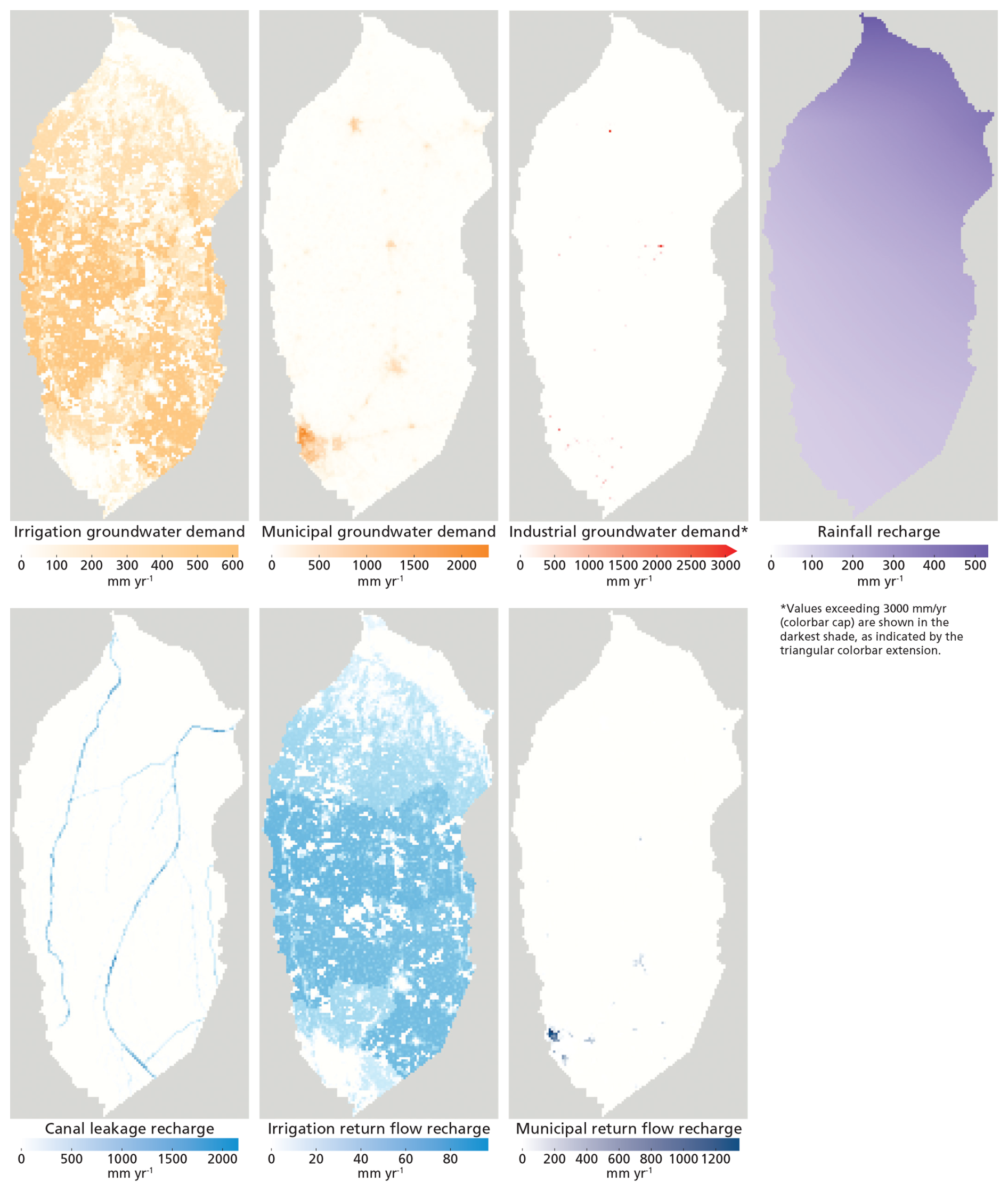
Figure A1 Spatial distribution of time-averaged annual recharge or demand of each component for the period 2000–2016, expressed in mm yr⁻¹.

A1 Irrigation groundwater demand

Irrigation groundwater demand was derived by estimating the amount of groundwater-irrigated hectares per cell multiplied by average yearly irrigation demand per hectare. The current spatial distribution of groundwater-irrigated agriculture was determined by resampling the Copernicus Global Land Cover map (Buchhorn et al., 2020) to calculate total agriculture per cell. This was adjusted using the ratio of total agriculture to groundwater-irrigated agriculture, based on 2011 census data (Government of India, 2011). A logistic growth curve (parameters: L=283 km³ yr⁻¹, k=0.0819, t0=1987) was constructed using national Indian groundwater withdrawal rates between 1950 and 2017 from the United Nations World Water Development Report 2022 (UN Water, 2022). The curve was normalised to the 2011 census reference year and fitted to hindcast groundwater withdrawal for irrigated agriculture over time. For the average yearly water demand per hectare, literature-based crop coefficients were applied. Crop water demand (transpiration) was calculated as potential evapotranspiration (ET) multiplied by the crop coefficient. Net irrigation demand was first calculated as the crop water requirement minus precipitation. This was subsequently converted to gross irrigation demand by accounting for irrigation inefficiencies (return flow), so that sufficient water is applied to satisfy crop transpiration while also generating return flow to the groundwater system to prevent soil salinisation. District-level crop distribution was sourced from the INTACH report (INTACH, 2017), with sugarcane (35.8 %), wheat (30.4 %), rice (9.5 %), and other crops (25.4 %) as the primary crops. Monthly crop coefficients were obtained from IWMI Research Report 140 (Cai et al., 2010). By combining district-wise crop data with crop coefficients, monthly crop coefficients per district were derived. Monthly irrigation water demand was calculated by multiplying potential evapotranspiration (PET) from the CRU TS dataset (Harris et al., 2020) by the district-level crop coefficient and subtracting precipitation (CRU TS). Only positive values were retained, as irrigation demand cannot be negative.

A2 Municipal groundwater demand

Regarding municipal groundwater demand we assumed all domestic water was sourced from groundwater. Demand was calculated by multiplying the number of inhabitants per cell by per capita water usage estimates from literature. Population data from WorldPop (Bondarenko et al., 2025) was used to get the spatial distribution of current inhabitants. The HYDE 3.2 population count dataset (Klein Goldewijk et al., 2017) was used to hindcast historical population trends spatially explicit with 2017 as the baseline. Per capita domestic water usage was taken from Joseph et al. (2021) for the years 1975 to 2015. This water usage has been linearly extrapolated backwards to 1800 where daily 25 L per capita was assumed.

A3 Industrial groundwater demand

Industrial groundwater demand was estimated using a dataset of industrial locations and their water discharge for a specific year (Uttar Pradesh Pollution Control Board, 2019). We assumed all industrial water was sourced from groundwater and applied a logistic trendline derived from national groundwater withdrawal rates (UN Water, 2022) to hindcast demand, assuming industrial locations remained constant over time.

A4 Rainfall recharge

Rainfall recharge was derived from the CRU TS dataset (1901–2024) (Harris et al., 2020), resampled to match our model grid. Recharge was calculated as the sum of monthly rainfall minus an estimated 2 % for surface runoff and minus monthly potential evapotranspiration (PET), with only non-negative values considered. This approach implicitly assumes that actual evapotranspiration approximates PET, which is considered reasonable because most precipitation occurs during the monsoon season when water availability is generally not limiting. For the period before 1900, the long-term rainfall recharge average was used due to data limitations, assuming no significant climate shifts.

A5 Canal leakage recharge

Canal leakage recharge was estimated by multiplying the canal area per cell by a leakage factor. Canal area per cell was derived from the India-WRIS dataset (India-WRIS, 2026), which provides canal locations, types, and names. Canal width was assumed to vary between 5 and 100 m depending on canal type. The leakage factor was based on Raza et al. (2013), who reported seepage losses of 0.32 L s⁻¹ per 100 m of unlined canal. Assuming an average canal width of 25 m in that study, this corresponds to an approximate leakage rate of 11 mm d⁻¹ m⁻² of canal area. Construction dates for individual canal sections were estimated from literature sources and used for hindcasting. Small-scale canal systems in the Indo-Gangetic Basin (IGB) date back to 16th century under Mughal rule (Jain et al., 2022). However, their contribution to regional groundwater recharge was likely minor compared with the extensive canal networks developed under British rule. We therefore quantified canal leakage only from 1830 (Eastern Yamuna Canal) and 1856 (Upper Ganga Canal), periods when such infrastructure began to significantly influence the groundwater balance and groundwater-surface water interactions.

A6 Irrigation return flow recharge

Irrigation return flow recharge was estimated by applying a groundwater return flow factor of 0.162 to the total irrigation demand. This return flow is derived from the total irrigation application described in Sect. A1 which is partitioned into consumptive use (crop transpiration) and return flow, with the latter thus added back to the groundwater as recharge. The return flow factor of 0.162 is based on Gupta and Deshpande (2004, as cited in van der Vat, 2018) who found an efficiency factor of 0.7 and a return flow percentage to groundwater of 54 % of total gross demand not transpired by the crop. Flood irrigation, the predominant irrigation method in the Indo-Gangetic Basin (IGB), leads to considerable evaporation losses but also generates substantial return flows to the groundwater system. Total irrigation demand consists of both groundwater and canal water demand. It was estimated using the same approach as the groundwater irrigation demand calculation; however, instead of the ratio of total agriculture to groundwater-irrigated agriculture, the total irrigated ratio derived from the 2011 census data published by the (Government of India, 2011) was applied. Hindcasting was performed using total irrigated area from HYDE 3.2 (Klein Goldewijk et al., 2017), averaged across the entire Indo-Gangetic Basin (IGB) at each time step.

A7 Municipal return flow recharge

Municipal return flow recharge was calculated by multiplying municipal demand by a leakage factor. The leakage factor varies depending on the distance to rivers. Municipal wastewater was assumed to discharge to rivers within 2.5 km and to ponds beyond that distance, with different infiltration rates applied accordingly. The wastewater discharge to rivers is assumed to have a leakage factor of 0.10. The wastewater discharged to pond is assumed to partly evaporate and partly infiltrate (factor 0.65).

Appendix B: Model performance evaluation

Figure B1 compares the observed groundwater heads with the simulated median groundwater heads for all observations at the monitoring wells. The blue dots represent the median of the posterior ensemble, while the grey error bars indicate the minimum and maximum simulated groundwater heads. Overall, the simulated and observed groundwater heads show good agreement (R²=0.86). The simulated heads are distributed around the 1:1 line (slope = 0.9), indicating no overall systematic over- or underestimation. Nevertheless, substantial deviations can occur for individual observations, with differences occasionally exceeding 10 m. Simulated error bars are larger with lower heads, which are mostly found at the southern region.

Figure B2 compares the observed Theil–Sen groundwater-level trends (m yr⁻¹), blue boxplot, with the simulated trends from the posterior ensemble (red boxplots). For the simulations, the minimum, median, and maximum Theil–Sen slopes at each observation well are grouped and shown. The observations exhibit considerable spatial variability, ranging from groundwater-level increases exceeding 0.25 m yr⁻¹ to declines greater than 1 m yr⁻¹, although the majority of wells show declining trends with a median of approximately −0.25 m yr⁻¹. The simulated ensemble reproduces a comparable overall range of trends, with almost all simulated trends remaining within the range of the observations. The median simulated trends span a narrower range and generally underestimate the magnitude of the observed groundwater-level declines. However, the lower bound (minimum trend per well) of the posterior ensemble closely matches the observed declining trends, indicating that a subset of the accepted model realizations captures these stronger declines well. The upper bound (maximum trend per well) mainly shows stable to slightly increasing groundwater levels and is still in the range of field observations.

Figure B3 presents observed groundwater heads together with the simulated posterior ensemble (minimum, median, and maximum) for the 12 wells with the longest observation records, i.e., up to 35 years. Overall, the simulations reproduce the long-term groundwater-level behaviour but do not capture all local temporal variations. The simulated groundwater heads generally exhibit smoother, more gradual changes than the observations, reflecting the dynamics of the larger scale regional model structure. Some wells, such as well_002, well_010, and well_048, show good agreement between observed and simulated groundwater heads. For other wells, including well_024 and well_031, the simulated trends are reproduced reasonably well, where the absolute groundwater heads are underestimated. Conversely, some wells, such as well_050, exhibit a much steeper observed groundwater-level decline than is simulated. Other wells, for example well_005, display pronounced local behaviour, an initial rapid groundwater-level rise followed by a sharp decline, that is not reproduced by the model. Such discrepancies are expected given the regional model's simplified representation of aquifer properties and recharge processes, which is designed to capture large-scale spatial patterns and long-term trends rather than site-specific behaviour. Oppositely, most of these wells are located in an urban environment and not a rural environment which makes them more vulnerable for operations under local conditions. This may explain some sharp declines of more than 1 m yr⁻¹.

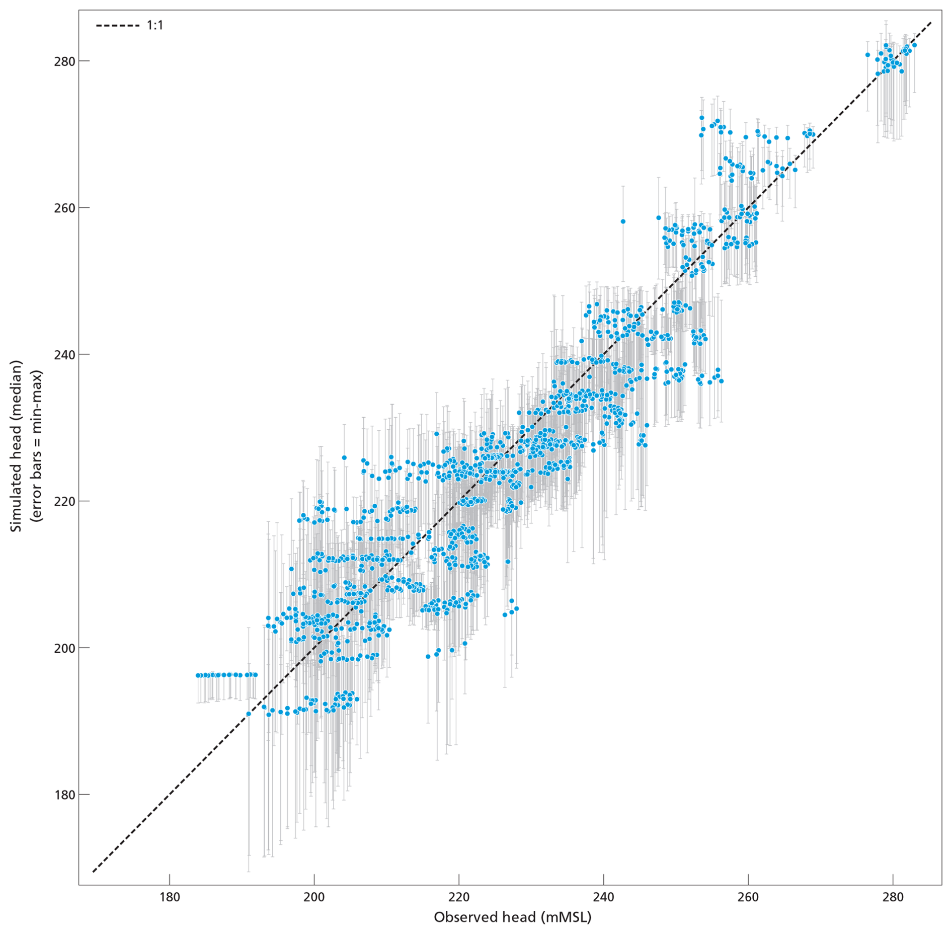
Figure B1 Observed groundwater head versus modelled median groundwater head in mMSL of the posterior ensemble (min–max) indicated as grey error bars.

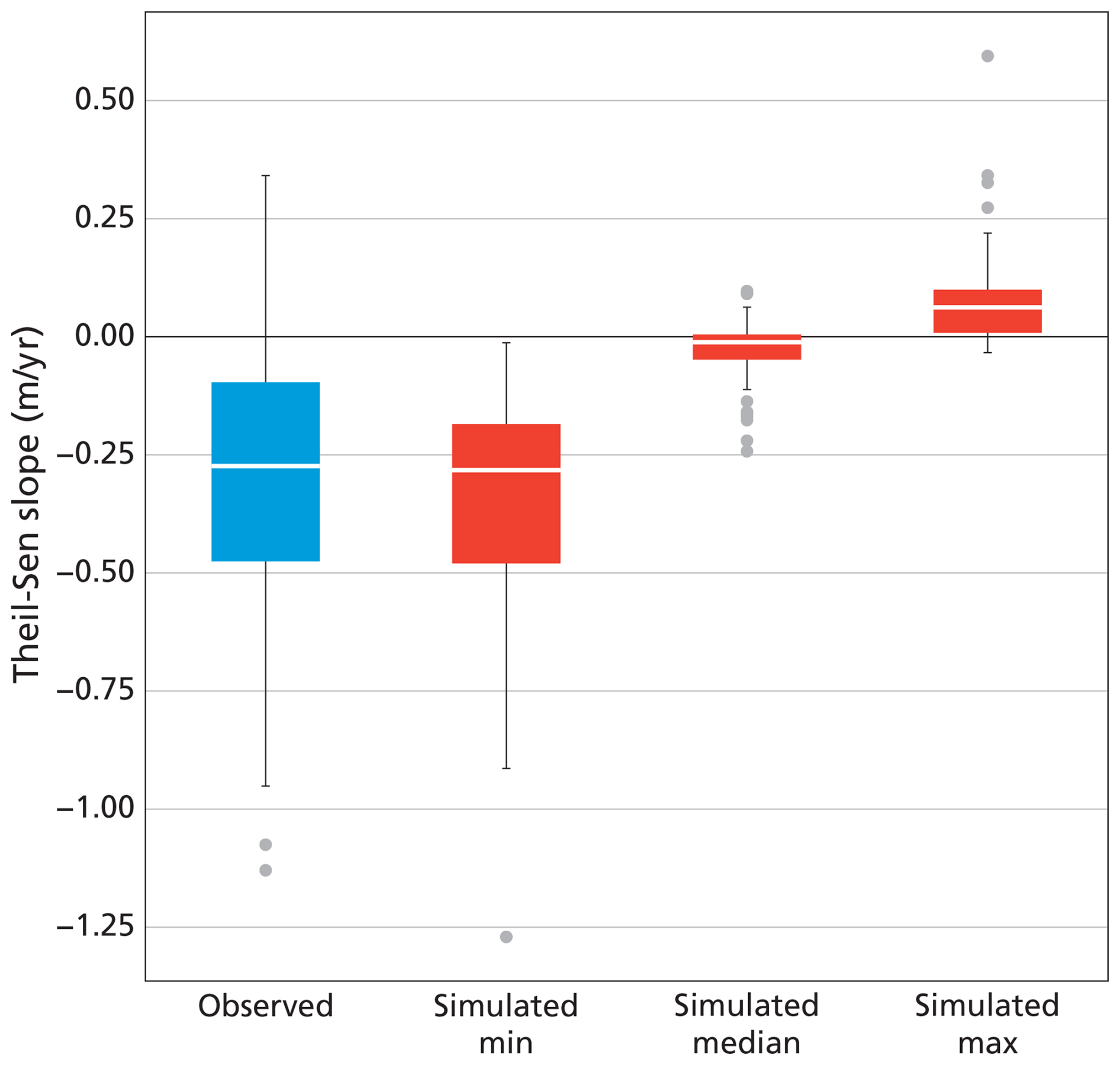
Figure B2 Boxplots of observed groundwater head Theil-Sen slope per observation well versus the modelled median, minimum and maximum groundwater head Theil-Sen slope in m yr⁻¹ of the posterior ensemble.

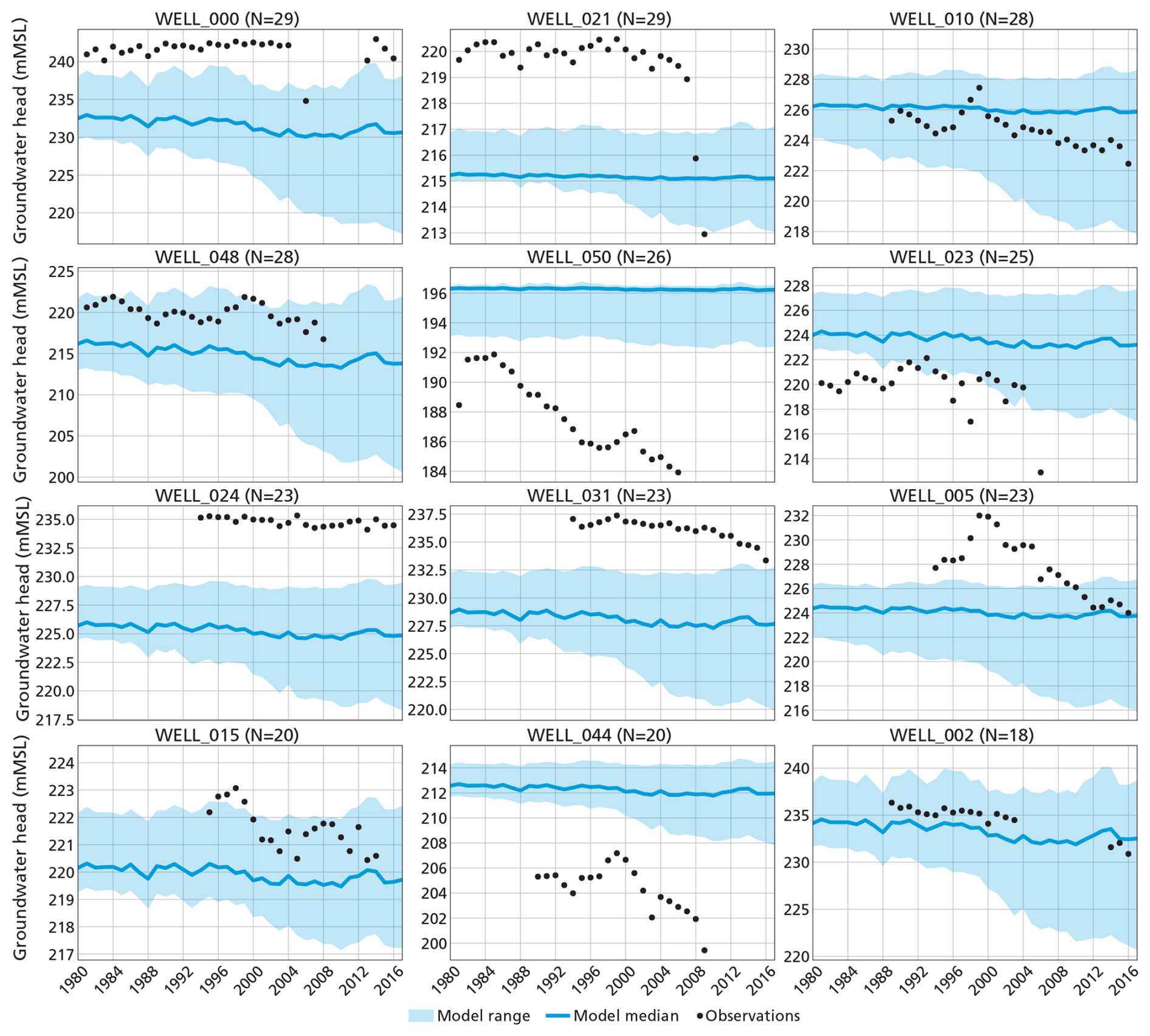
Figure B3 Observed groundwater head (dots) versus modelled groundwater head of the posterior ensemble (min, median, max) for the 12 longest well observation series. Blue lines are modelled median groundwater heads and in light blue the modelled ranges between minimum and maximum of the posterior ensemble.