Technical note: A physically based correction of WRF temperature using atmospheric lapse rates for high-resolution hydrological simulations in a glacierized catchment

This technical note presents a physically based post-processing workflow for correcting coarse-resolution regional climate model output used to force high-resolution hydrological models in high-elevation, glacierized catchments. The Weather Research and Forecasting (WRF) model was used to dynamically downscale the 20th Century Reanalysis Version 3 (20CRv3; 1° × 1°, 3-hourly) to a spatial resolution of 2 km and an hourly temporal resolution for the period 1969–2015. Evaluation of WRF output in the upper Kauner Valley (Austria) revealed a pronounced cold bias in the diagnosed 2 m temperature at elevations above 2600 m above sea level, which was attributed to the coarse representation of snow- and ice-covered surfaces and their influence on land-atmosphere interactions. To address this limitation, we developed a novel post-processing workflow that derives hourly temperature lapse rates directly from the WRF atmosphere using temperature and geopotential height fields from multiple eta levels. These lapse rates are subsequently used to reconstruct near-surface temperatures from the first atmospheric model level, thereby reducing the influence of surface-related biases. In addition, a sequential thermodynamically consistent correction of relative humidity was applied using the corrected temperature fields. The proposed approach was evaluated against observations from four meteorological stations spanning an elevation gradient of nearly 900 m and through hydrological simulations with the physics-based WaSiM model. Corrected hourly temperatures showed substantially improved agreement with observations, whereas simulations driven by uncorrected WRF data failed to adequately reproduce observed cryospheric and hydrological dynamics. The temperature correction significantly improved the simulation of snow accumulation and melt, glacier mass balance, snow cover dynamics, and streamflow. Furthermore, the thermodynamically consistent correction of relative humidity enhanced late-summer streamflow during periods of maximum glacier melt. Evaluation against homogenized station observations demonstrated that the corrected temperature product preserves long-term regional warming trends over a period of 42 years, indicating its suitability for climate impact assessments. The results show that the proposed workflow effectively reduces temperature biases associated with coarse-resolution land-cover representation while maintaining physical consistency among meteorological variables. Because the method relies on atmospheric lapse rates derived from the regional climate model itself rather than long-term local observations, it provides a transferable alternative to empirical bias-correction approaches and a robust framework for hydrological and climate impact studies in glacierized mountain environments.

1 Introduction

The European Alps are particularly affected by climate change, as observed temperature increases are approximately twice the global average, resulting in an average warming of 1.8 °C since 1880 (Kotlarski et al., 2023). However, this trend has not been linear since pre-industrial times, as warming has significantly accelerated in the last 30 years (Nigrelli and Chiarle, 2023), with considerable consequences for the entire Alpine geosystem and its inhabitants (Matiu et al., 2021; Marcolini et al., 2017, 2019; Morin et al., 2021; Magnusson et al., 2020). In addition, the accelerated warming rates of the European Alps are probably leading to heavier rainfall intensities and, consequently, to greater and sudden floods (Wilhelm et al., 2022). Understanding the drivers of past climate-induced changes in the hydrological response of Alpine catchments is relevant for developing future adaptation strategies for water resources and risk management.

The study of climate-induced long-term changes mainly depends on station observations. However, observations dating back to the last Little Ice Age (LIA) around 1850 are limited in both space and time in the Alpine region. Homogenized temperature and precipitation records are even available before 1850 (Auer et al., 2005, 2007), but they are not equally distributed and mainly represent lower-laying areas of the Alpine region (van Tiel et al., 2022). The linear extrapolation of these temperature records to higher elevations is problematic because several studies have found different trends in the elevation-dependent warming (e.g., Rangwala and Miller, 2012; Kuhn and Olefs, 2020). High-resolution Regional Climate Models (RCMs) bridge this spatiotemporal gap by dynamically downscaling global reanalysis products to a much finer grid resolution of a few kilometers, thereby permitting the simulation of convection. To account for the complex orography of the Alps, multiple studies have demonstrated the benefits of high-resolution RCMs for regional climate change studies in the European Alps (Gómez-Navarro et al., 2015; Warscher et al., 2019). A frequently used model for long-term atmospheric simulations is the Weather Research and Forecasting (WRF) model (Powers et al., 2017). The main advantage of dynamical downscaling with atmospheric models is the physical consistency, which means that all fields are downscaled simultaneously, so the interdependencies between downscaled variables are preserved (Berg et al., 2024). The major disadvantage is the high computational cost of running the WRF model. For the study domain considered here (approximately 24 400 km²), centennial simulations at 2 km horizontal resolution can take several months, even on high-performance computing systems.

Although many high-resolution WRF climate simulations have a spatial resolution of a few kilometers (Gómez-Navarro et al., 2015; Warscher et al., 2019; Velasquez et al., 2020), they are still far too coarse for resolving localized precipitation patterns or small-scale processes such as snow redistribution in high-elevation areas (Berg et al., 2024). Moreover, the simulated near-surface heat fluxes depend on the spatial resolution of the WRF elevation model and the resolution and accuracy of land cover classes (i.e., land-atmosphere interactions). In addition, elevation-dependent processes, such as temperature and precipitation lapse rates, are not sufficiently resolved by RCMs at the sub-kilometer scale due to their coarser topography, which often under-represents terrain features. Comprehensive correction procedures are therefore necessary to rescale and correct the coarse-scale RCM data to a much finer spatial resolution in mountainous regions, as usually required by distributed hydrological models. Velasquez et al. (2020) developed a three-step procedure for bias-correcting WRF precipitation over a complex terrain in the Swiss Alps. This approach explicitly considers orographic characteristics. The first step is the separation of precipitation by orographic characteristics; the second is the adjustment of daily precipitation with very low intensity; and the third is the application of empirical quantile mapping (EQM). EQM consists of adjusting the quantile values from a simulation to those from the observations through a transfer function (Velasquez et al., 2020). Therefore, the EQM method is based on the availability of meteorological time series with sufficient temporal coverage and quality. However, meteorological observations are particularly limited in mountainous areas, especially in relation to reliable precipitation records from high altitudes (> 2000 m a.s.l.; Foehn et al., 2018). In combination with the non-stationarity of meteorological observations (Teutschbein and Seibert, 2012), the evaluation of bias correction methods in data-scarce mountainous regions is particularly challenging.

Hydrological models can serve as an additional validation method for the reliability of bias corrections, as adjusted forcing data will affect the quality of hydrological model results (Teutschbein and Seibert, 2012; Shrestha et al., 2017; Hakala et al., 2018; Hofmeister et al., 2023; Meyer et al., 2019). It can be assumed that a bias correction is expected to yield more realistic and plausible hydrological model results than a model forcing based on the uncorrected RCM (Teutschbein and Seibert, 2012; Meyer et al., 2019). However, the focus should not only be on good and plausible streamflow results for alpine catchments, but also on the reliability of the other hydrological processes (Tuo et al., 2018; Hofmeister et al., 2023; Schaffhauser et al., 2025). Mainly, elevation-dependent processes, such as snowfall and melt generation, depend on a reliable representation of temperature and precipitation lapse rates in mountainous regions (Hakala et al., 2018; Hofmeister et al., 2023; Berg et al., 2024; Meyer et al., 2019). Although most of the previous evaluations of bias correction methods with hydrological models focused on monthly or daily model results (Teutschbein and Seibert, 2012; Shrestha et al., 2017; Hakala et al., 2018; Meyer et al., 2019), Faghih et al. (2022) found that even the diel cycle of variables simulated by RCMs is biased, which raises issues about the necessity of correcting such biases prior to streamflow simulations at the subdaily timescale. They recommend correcting the diel cycle of RCM variables before using them for hydrological simulations to accurately represent the diel cycle of summer streamflow in small catchments (i.e., < 500 km²; Faghih et al., 2022).

The objective of this technical note is to develop and evaluate a physically based post-processing workflow for reducing biases in coarse-resolution regional climate model output used to force high-resolution hydrological models in high-elevation, glacierized catchments. We focus primarily on near-surface air temperature, as snow and glacier processes are highly sensitive to its spatiotemporal variability. Rather than relying on empirical bias-correction techniques, we derive hourly temperature lapse rates directly from the free WRF atmosphere and use them to reconstruct near-surface temperatures from the first atmospheric model level. This approach aims to reduce biases arising from the coarse representation of snow- and ice-covered surfaces and associated land–atmosphere interactions in convection-permitting WRF simulations.

In addition, we apply a sequential, thermodynamically consistent correction of WRF relative humidity based on the corrected temperature fields. This step is particularly relevant for energy-balance-based snow and glacier melt modeling, where latent heat fluxes contribute substantially to the surface energy balance. In contrast, no post-processing corrections are applied to shortwave radiation or wind speed. Physics-based hydrological models such as SNOWPACK (Lehning et al., 2002), openAmundsen (Strasser et al., 2024), and WaSiM (Schulla, 2021) already account for scale-dependent topographic effects on radiation and, where applicable, include representations of wind-driven snow redistribution.

The proposed workflow is evaluated using a multi-data approach in the highly glacierized upper Kauner Valley (eastern European Alps). In addition to statistical validation against meteorological observations, we assess the impact of the corrected forcing data on simulations of snow cover, snow water equivalent, glacier mass balance, glacier extent, and streamflow using the fully distributed, physics-based hydrological model WaSiM. Evaluations are performed across temporal scales ranging from hourly variability to multi-decadal trends spanning up to 42 years.

Beyond introducing a novel temperature correction method, this technical note highlights the importance of physically consistent meteorological forcing data for hydrological and cryospheric modeling in complex mountain terrain. The study provides insights into the interactions among atmospheric forcing, snow and glacier dynamics, and catchment hydrology, and demonstrates the need for accurate representations of temperature and humidity fields in climate impact studies of glacierized catchments.

2 Material and methods

2.1 Study site

The research site is located in the upper Kauner Valley in the Tyrolean Alps (Austria), has an elevation range of 1810–3535 m a.s.l. (Altmann et al., 2020), and is mainly drained by the Fagge River, a tributary of the upper Inn River system. The drainage area of the Fagge at the stream gauge Gepatschalm (GA), south of the Gepatsch reservoir (Fig. 1), covers about 54 km². The actual drainage in this study is slightly larger (62 km²), as it extends beyond the stream gauge GA and the catchment is closed at the inflow to the Gepatsch reservoir. The streamflow regime of the Fagge is strongly influenced by snow and glacier melt, resulting in distinct seasonality with low flows in winter and high flows in summer. The glacier coverage is relatively high with a 30 % fractional cover in 2015 (Buckel and Otto, 2018), but has declined from 39 % in 1969 according to the first Tyrolean Glacier Inventory (Patzelt, 2013). Accordingly, the entire geosystem of the upper Kauner Valley has undergone profound changes over the respective period, as investigated in multiple studies (e.g., Altmann et al., 2020, 2024; Piermattei et al., 2023). In 2020, scree (vegetation cover < 20 %) was the dominant land cover at 32 %, closely followed by glacier cover at 27 %, which corresponds to a reduction of fractional glacier cover by 2 % in only five years. Rocks with vegetation cover about 12 % of the upper Kauner Valley, followed by grassland and dwarf shrubs. Subalpine coniferous forest only covers 1.3 % of the research area along the valley bottom. The land cover classification was carried out by Ramskogler (2023). With several existing long-term hydrometeorological observation stations (Fig. 1), the upper Kauner Valley is an ideal study site for hydrological model applications (e.g. Förster et al., 2016; Rogger et al., 2017; Pesci et al., 2023). Although no continuous glacier mass balance data are available, the high-quality hydrometeorological instrumentation, which is often even better than that of the United States Geological Survey Benchmark Glacier Project (Schaffhauser et al., 2025), makes the upper Kauner Valley an ideal case study for cryohydrological research.

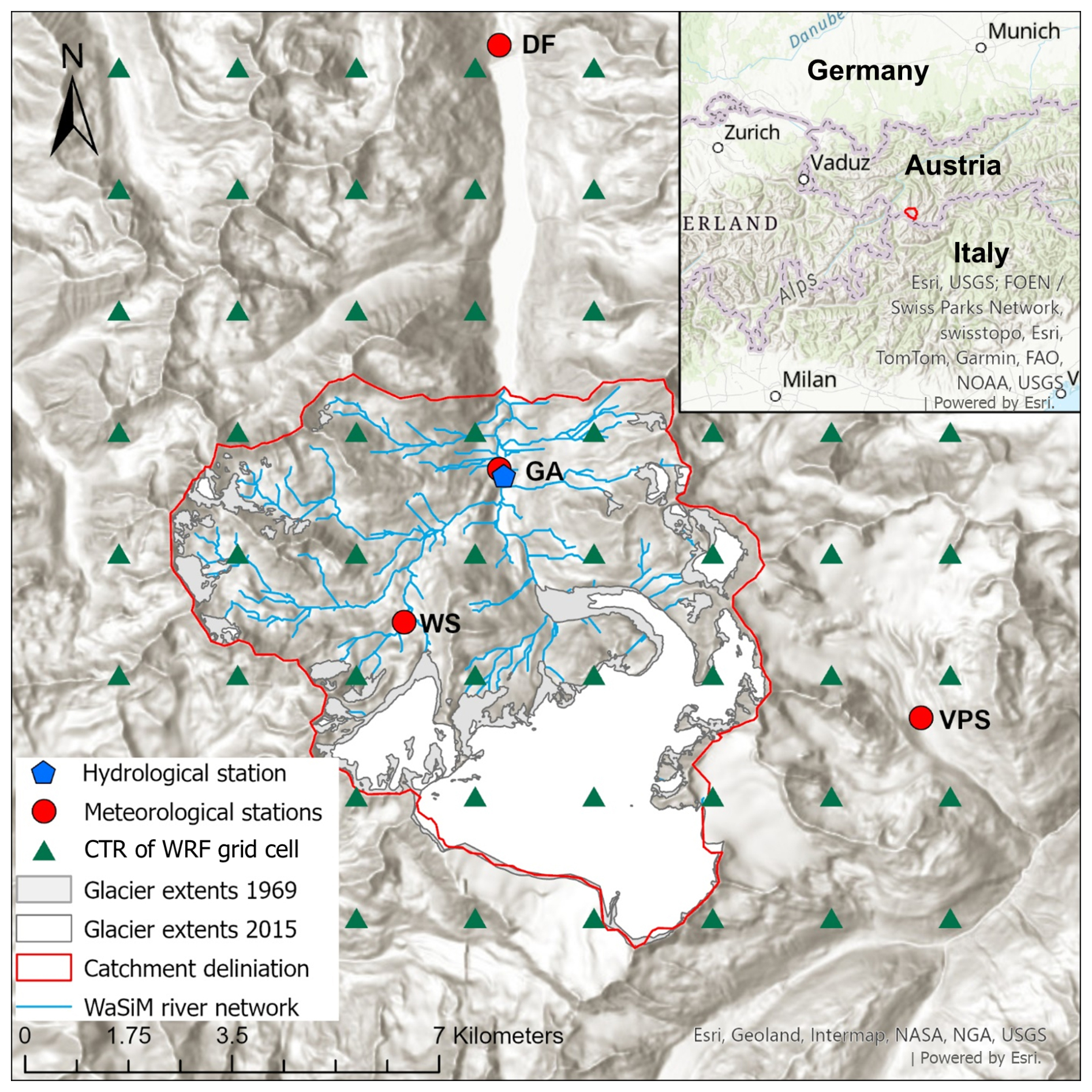
Figure 1 Overview map of the research area the upper Kauner Valley in Tyrol (Austria). Green triangles illustrate the center of the 2 km WRF grid cells. Meteorological stations are indicated with red circles. Hydrological stations are represented with a blue symbol. Glacier extents are plotted for 1969 from the first Tyrolian Glacier Inventory (GI 1) and 2015 from the fourth inventory (GI 4). Catchment delineation and river network were computed based on the official digital elevation model of Tyrol from 2006, which is available from the Province of Tyrol and downloadable at the following URL: https://www.data.gv.at/, last access: 25 September 2026.

2.2 Hydrometeorological observation data

High-resolution (i.e., 15 min intervals) streamflow data at gauge Gepatschalm (GA) were provided by TIWAG-Tiroler Wasserkraft AG, the local hydropower plant operator, for the period 1971 to 2022. Larger data gaps of several months mainly affect the first four years of streamflow observations at GA. Most of the meteorological stations in the upper Kauner Valley (Dammfuss, Gepatschalm, Weisssee), listed in Table 1, are also operated by TIWAG. The TIWAG temperature time series includes only a low fraction (i.e., < 1 %) of data gaps. The Bavarian Academy of Science operates multiple stations at the nearby Vernagtferner. The main station at Vernagt Pegel has recorded hourly meteorological variables since 1975 and is the highest station in the region (2640 m a.s.l.) with the longest temporal coverage. Due to some failures of the station and sensor, the temperature time series has about 7 % of data gaps for the period 1975–2015. The meteorological station in Vergoetschen (1269 m a.s.l.) is operated by the HD-Tyrol and is located in the lower Kauner Valley. This station was chosen to correct the precipitation frequency of the regional climate model (WRF) due to its high reliability and long temporal coverage (since 1895) of daily precipitation measurements. Longer data gaps at the VG stations are mainly due to World War II. As all stations are still in operation, only the start year of the observation is given in Table 1. Unfortunately, there is no overlap in time with the meteorological station installed in 2017 on the Weissseespitze (Stocker-Waldhuber et al., 2022), which is located at an altitude of 3500 m in the upper Kauner Valley.

Table 1 Metadata of the meteorological stations and statistics about the data availability of meteorological observations. The coordinates are given as UTM coordinates for zone 32N (epsg code: 32632). Although several other meteorological variables may be available for the stations, we only indicate the variables used in this technical note.

2.3 Snow observation data

The snow observation data are used to evaluate the simulation results of the hydrological model at the point scale using station-based snow water equivalent (SWE) data and at the catchment scale using binary snow cover data retrieved from an optical remote sensing product (i.e., MODIS).

2.3.1 Calculation of SWE data

Snow depth measurements within the research site were available only at the TIWAG station Weisssee since 2007. To transform daily snow depth to daily SWE, we applied the recently developed deltaSnow model (Winkler et al., 2021). SWE is modeled using a process-based multi-layer approach, incorporating empirical regression models based on the relationship between density and diverse at-site parameters (Winkler et al., 2021). Accordingly, the ΔSnow model lies between simple empirical regression models, such as Jonas et al. (2009), and full thermodynamic models, such as SNOWPACK (Lehning et al., 2002) or Crocus (Vionnet et al., 2012), offering a physically based but data-sparse SWE estimator. The ΔSnow model does not require meteorological forcing, such as temperature or precipitation data. This is particularly useful where SWE measurements are sparse, but snow depth records are available, as is the case in the upper Kauner Valley. We used the same model parameters as published by Winkler et al. (2021), which were calibrated and evaluated against station observations from different altitudes and climatic regions of the European Alps.

2.3.2 Snow cover data

Daily, nearly cloud-free MODIS snow cover maps are available for the entire European Alps at 250 m grid resolution since summer 2002 (Matiu et al., 2019a, b). Despite the relatively coarse grid resolution compared to other optical snow products (e.g., Landsat, Sentinel 2), MODIS snow cover maps can provide valuable information on the evolution of seasonal snow cover at high temporal resolution (i.e., daily). Due to their high temporal resolution and global coverage, MODIS snow cover data have already been used in many studies focusing on hydrological modeling in high-elevation catchments (e.g., Duethmann et al., 2014). After bilinear resampling and cropping the MODIS snow cover maps to the respective catchment resolution (i.e., 25 m) and domain, we set glaciated raster cells to no data as they are permanently snow-covered and would bias the comparison with the snow cover simulations of the hydrological model. We use glacier extents from the third Tyrolean glacier inventory from 2006 (Abermann et al., 2012). To ensure consistency between observed and simulated snow cover maps, we set the same grid cells to no data in both products and normalize the fractional snow-covered area (fsca) values from 0 (no snow) to 1 (completely snow-covered). Snow cover data with higher spatial resolution from Sentinel 2 (Hofmeister et al., 2022) could not be used for this case study because there is insufficient overlap between the data. The WRF data ends in 2015, the year Sentinel 2 was launched.

2.4 Dynamical downscaling with WRF

The model forcing of the hydrological model is generated with the Weather Research and Forecasting (WRF) model (version 4.3), which is based on fully compressible and non-hydrostatic equations (Skamarock et al., 2008). The global Twentieth Century Reanalysis version 3 (20CRv3) data set (Compo et al., 2011; Giese et al., 2016; Slivinski et al., 2019), with spatial and temporal resolutions of 1° × 1° and 3 h, is used as the driving data (initial and boundary conditions). The simulation is performed in three nested domains, with a grid spacing of 18 km (domain 1), 6 km (domain 2), and 2 km (domain 3). The WRF domain with 2 km resolution covers an area of about 24 416 km². The simulated data in domain 3 are stored at 1 h intervals. The vertical discretization is based on 49 virtual atmospheric layers, the so-called eta levels, which allows the WRF model to resolve atmospheric flow near complex terrain more accurately. The Yonsei University scheme is selected to calculate the planetary boundary layer (Hong et al., 2006). Further information on the WRF model configuration can be found in Altmann et al. (2024). The WRF grid cells considered in this case study cover an area of about 200 km², including parts of the neighboring valleys (Fig. 1).

We use the Noah land surface model (LSM), one of the most widely used land surface components in WRF, which plays a crucial role in simulating interactions between the land surface and the atmosphere. The LSM calculates the energy and mass transfer at the ground interface, providing bottom boundary conditions to the atmospheric model WRF (Tomasi et al., 2017). The Noah LSM is based on 24 land use categories originating from the United States Geological Survey (USGS; Anderson et al., 1976). From the 24 land cover categories, only seven are represented in the WRF domain of the upper Kauner Valley (Fig. S1 in the Supplement): Woodland Mosaic, Grassland, Shrubland, Evergreen Needleleaf, Wooded Wetland, Wooded Tundra, and Snow or Ice. The most frequent category of the WRF Kauner Valley domain is Wooded Tundra (15 grid cells), followed by Snow or Ice (11 grid cells). The latter category means permanent snow- and ice-covered areas where snow and ice cover persist for at least ten months of the year, typically exceeding 60 % of the area. This category signifies a large presence of snow and ice as a permanent landscape feature (Anderson et al., 1976). The category Snow or Ice covers most of the higher-elevation research site (i.e., > 2900 m a.s.l. in Fig. S1), including the Gepatsch glacier. A separate map of the WRF land use categories at 2 km resolution is shown in the Supplement (Fig. S2).

Figure 2 shows the relation between grid cell surface elevation (m) and simulated temperatures at different model levels averaged over a test period of three months (i.e., from August to November) stratified according to the land cover per grid cell. The temperatures shown correspond to different eta levels, the surface (or skin) temperature (TSK), and the diagnosed 2 m above-ground temperature (T₂). The first model level (Fig. 2c) corresponds on average to an altitude of about 17 m above the ground surface over the three-month test period. It is computed by subtracting the mean WRF geopotential height of eta level 1 from the mean WRF surface height (2785 m) of the upper Kauner Valley. Eta level 49 (Fig. 2f) has an average altitude of approximately 30 km above the ground surface. The TSK and T₂-elevation relationships (Fig. 2a and b) show substantially lower temperatures over snow- and ice-covered grid cells, together with considerable scatter. This suggests that the simulated temperatures are strongly influenced by surface properties, with the cooling effect of snow and ice extending from the surface to the near-surface air represented by T₂. The elevation gradients (both with and without snow) of TSK and T₂ are higher than at the next higher eta levels. In this context, a higher gradient means a larger change in temperature with elevation. The free atmosphere is typically defined in WRF as the part of the atmosphere above the planetary boundary layer, where turbulent mixing from the surface becomes negligible. However, the exact eta level or geopotential height that marks the transition to the free atmosphere is not fixed. It varies dynamically in space and time, depending on surface properties, atmospheric stability, and time of day (Hong et al., 2006).

From eta level 1 to eta level 20 (Fig. 2c, d), WRF temperature exhibits an almost perfectly linear relationship with surface elevation and very little scatter. This indicates that temperatures at these levels are predominantly governed by a nearly uniform domain-wide lapse-rate structure, with only minor influence from land-cover or snow-cover differences. Because all panels in Fig. 2 share a common y-axis span, this weakening relationship is directly visible as a progressive flattening of the fitted slope with height: above eta level 20 the regression line becomes increasingly shallow, and by eta level 30 and eta level 49 the data points collapse onto an almost horizontal band, indicating that surface elevation no longer exerts a discernible control on temperature at these levels. This behavior reflects the decreasing influence of terrain with height: the lower eta levels closely follow the terrain, whereas higher eta levels become increasingly horizontal and sample the free atmosphere, where temperature variations are controlled more by large-scale atmospheric structure than by the underlying surface elevation. The lapse rate at eta level 1 equals −0.78 °C 100 m⁻¹, i.e., it is higher than in the free atmosphere (which corresponds to −0.65 °C 100 m⁻¹) for the three-month test period, and it decreases steadily with height, reaching −0.32 °C 100 m⁻¹ at eta level 20, and approaching zero (−0.02 and −0.00 °C 100 m⁻¹, respectively) at eta levels 30 and 49.

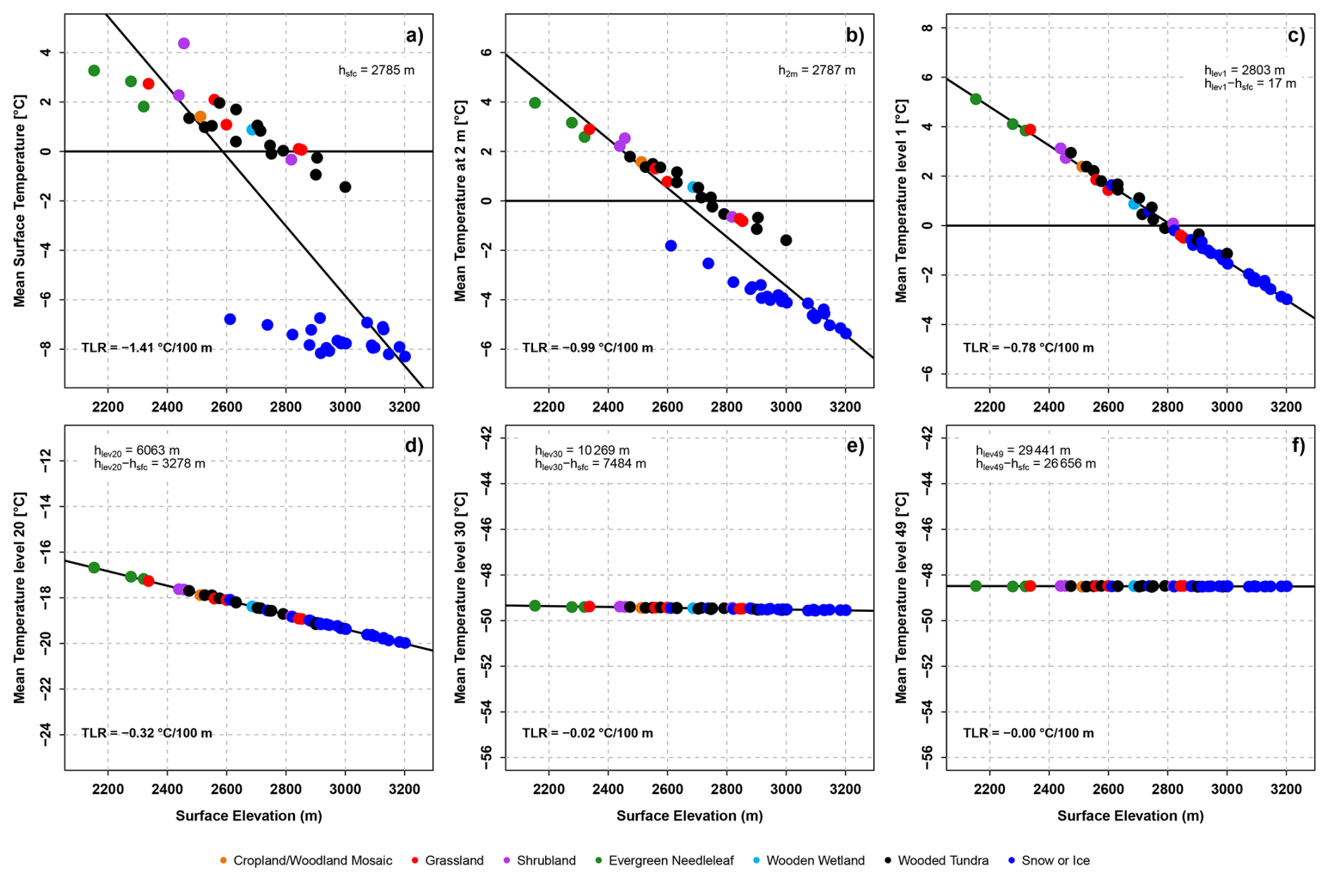
Figure 2 Mean WRF temperature for different land use categories and surface elevations (m) for the Kauner Valley domain covering a test period of three months. The diagonal black line shows the linear gradient between elevation and temperature obtained by least-squares fitting to all data points. The numbers in the subplots indicate the respective geopotential height, the height above ground, and the temperature lapse rate (TLR). The horizontal black line indicates the freezing level at 0 °C. The y-axes of all six panels share the same 14 °C y-axis span, each centered on that panel's own mean.

2.4.1 Correction of the WRF temperature

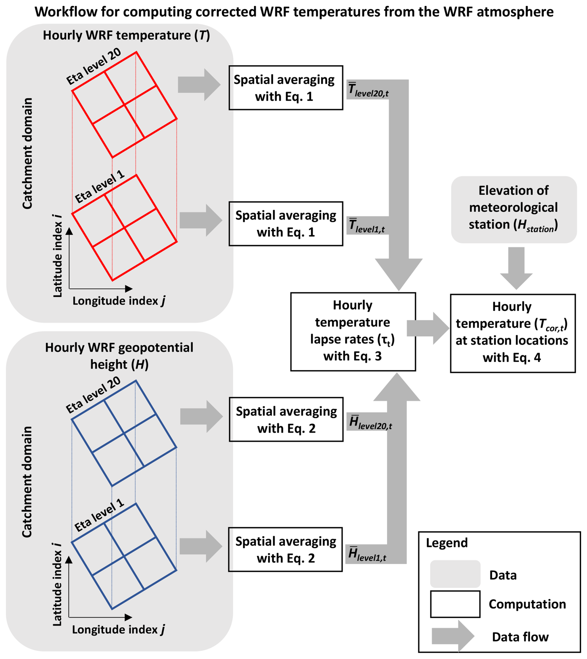
Figure 3 Developed workflow for computing corrected WRF temperatures from the multidimensional WRF atmosphere data.

The WRF temperature is adjusted using a three-step approach on hourly time series to account for sub-daily changes in temperature lapse rates (TLRs). As correcting WRF temperatures is a complex task due to the multidimensionality of the data, we have summarized the individual processing steps of the developed workflow in Fig. 3. First, we compute spatial averages of the hourly temperature of eta levels 1 and 20 over the 200 km² domain of the upper Kauner Valley by applying Eq. (1):

$$\begin{array}{}\text{(1)}& {\stackrel{\mathrm{‾}}{T}}_{\text{level}X,t}={\displaystyle \frac{\mathrm{1}}{N}}\sum _{i=\mathrm{1}}^M\sum _{j=\mathrm{1}}^{L}T(t,i,j)\end{array}$$

where ${\stackrel{\mathrm{‾}}{T}}_{\text{level}X,t}$ is the spatial mean of temperature [°C] of the respective eta level (levelX) at time t. In our case, time t has an hourly resolution. $T(t,i,j)$ is the variable value at time t, latitude index i, and longitude index j. M is the total number of latitude points, and L is the total number of longitude points. N is the total number of spatial grid points. As the WRF grid of the Kauner Valley has 7 rows (M) and 7 columns (L), a total of 49 grid cells (N) are considered in Eq. (1). Spatial averaging reduces TLRs' dependence on WRF land cover types, especially at lower eta levels.

We use the same approach to calculate the spatial averages of the hourly geopotential height following Eq. (2):

$$\begin{array}{}\text{(2)}& {\stackrel{\mathrm{‾}}{H}}_{\text{level}X,t}={\displaystyle \frac{\mathrm{1}}{N}}\sum _{i=\mathrm{1}}^M\sum _{j=\mathrm{1}}^{L}H(t,i,j)\end{array}$$

where ${\stackrel{\mathrm{‾}}{H}}_{\text{level}X,t}$ is the spatial mean of geopotential height [m a.s.l.] of the respective eta level (levelX) at time t. As the temperature and geopotential height grids have the same spatiotemporal dimensions, the variables of ${\stackrel{\mathrm{‾}}{H}}_{\text{level}X}(t,i,j)$ are identical to ${\stackrel{\mathrm{‾}}{T}}_{\text{level}X}(t,i,j)$.

In a second step, we compute the hourly TLRs based on the spatial averages (from Eqs.1 and 2) using Eq. (3):

$$\begin{array}{}\text{(3)}& {\mathit{\tau }}_t={\displaystyle \frac{{\stackrel{\mathrm{‾}}{T}}_{\text{level\_}\mathrm{20},t}-{\stackrel{\mathrm{‾}}{T}}_{\text{level\_}\mathrm{1},t}}{{\stackrel{\mathrm{‾}}{H}}_{\text{level\_}\mathrm{20},t}-{\stackrel{\mathrm{‾}}{H}}_{\text{level\_}\mathrm{1},t}}}\end{array}$$

where τ_t is defined as a signed quantity [°C m⁻¹] at time step t and is typically negative, ${\stackrel{\mathrm{‾}}{T}}_{\text{level\_}\mathrm{20},t}$ [°C] is the spatial average temperature $\stackrel{\mathrm{‾}}{T}$ of eta level 20 at time step t, and $\stackrel{\mathrm{‾}}{H}$ is the spatial average altitude of the eta levels in m a.s.l. (i.e., the geopotential height). Eta level 20 corresponds to a geopotential height of about 6000 m a.s.l., which represents a mean height above ground of 3278 m. Given the objective of a transferable bulk lapse rate derived from atmospheric model levels, we have chosen eta levels 1 and 20 for two reasons: eta level 1 still includes minor temperature differences due to the land-atmosphere interactions (Fig. 2c), which are more pronounced in summer (Fig. S3a). On the contrary, eta level 20 does not show any scattering around the regression line (Fig. 2d) or any season dependencies (Fig. S3d) that is caused by surface properties (i.e., land cover and snow cover), which indicates a horizontally uniform lapse rate structure in the domain. Accordingly, the higher variability and magnitudes from lower levels will be averaged out by the upper levels. Although the transition of mean TLR from eta level 1 to 20 is not linear, we apply the linear function of Eq. (3) for efficiently computing mean TLR over the entire altitude range. Considering all eta levels from 1 to 20 would significantly increase the computational demand. The red line in Fig. 4 represents the mean TLR between eta levels 1 and 20. Including eta level 1 in the linear equation ensures that temperature fluctuations are not completely decoupled from the surface and topography of the research area. The TLRs of Fig. 4 are computed between two neighboring eta levels and illustrate the sensitivity of TLRs to eta level selection. This calculation was based on the mean temperature of all grid cells in the Kauner Valley for each level. Except for the lapse rate between the first two eta levels, all other lapse rates up to eta level 20 range from −0.52 to −0.67 [°C (100 m)⁻¹]. Further information on the justification of the eta level range section and the use of a linear gradient can be found in the Results (Sect. 3.1).

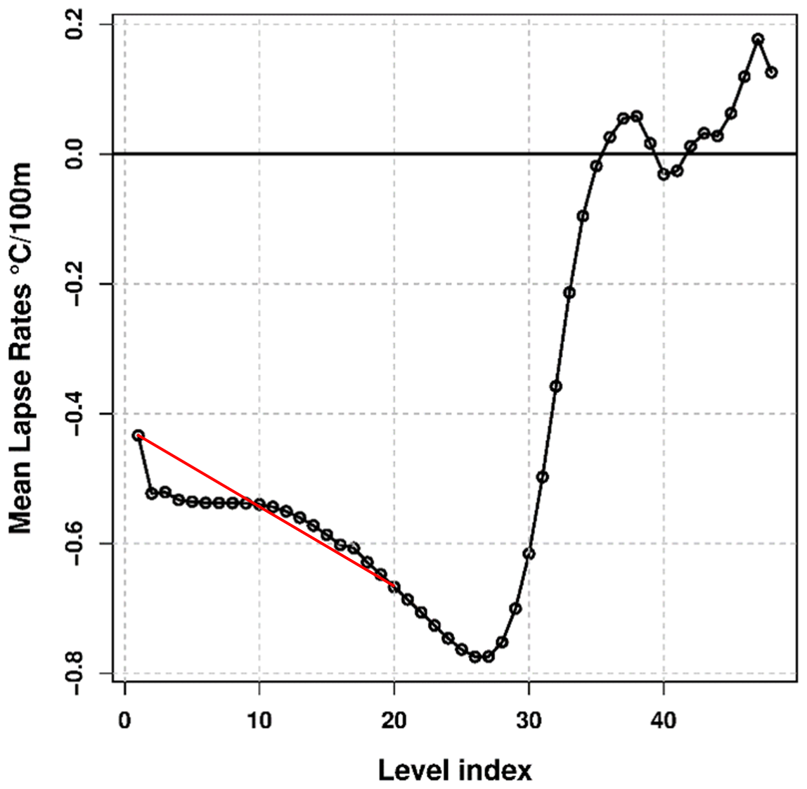
Figure 4 Mean WRF temperature lapse rates in °C (100 m)⁻¹ per eta level. The TLRs are computed for two pairs of consecutive eta levels. The red line represents a linear approximation of the lapse rates based only on the lapse rates from eta levels 1 and 20. The mean elevation of eta level 1 is about 2800 m a.s.l., about 6100 m a.s.l. for eta level 20, and about 10 300 m a.s.l. for eta level 30. The elevation range of the Kauner Valley is from 1810 to 3535 m a.s.l.

In the third step, the hourly corrected WRF temperature (T_cor) [°C] at station elevations is computed by extrapolating the temperature at eta level 1 to the station height using the hourly temperature lapse rate. The corrected temperature at time step t is calculated by Eq. (4):

$$\begin{array}{}\text{(4)}& T_{\text{cor},t}=T_{\text{level\_}\mathrm{1},t}+{\mathit{\tau }}_t\cdot (H_{\text{station}}-H_{\text{level\_}\mathrm{1}})\end{array}$$

where H_station represents the station elevation in m a.s.l. and H_{level_1} the mean geopotential height of the eta level 1 (i.e., 2803 m a.s.l.).

We compute the overall mean TLR using Eq. (5):

$$\begin{array}{}\text{(5)}& {\stackrel{\mathrm{‾}}{\mathit{\tau }}}_t={\displaystyle \frac{\mathrm{1}}{Y}}\sum _{t=\mathrm{1}}^Y\mathit{\tau }\left(t\right)\end{array}$$

where ${\stackrel{\mathrm{‾}}{\mathit{\tau }}}_t$ is the mean TLR [°C m⁻¹] over time and Y is the total number of time steps. Accordingly, the computed mean TLR is −0.57 °C 100 m⁻¹ from eta level 1 to 20 over the period 1973–2015. The summer TLR (i.e., May to September) is with −0.58 °C 100 m⁻¹ slightly larger than the winter TLR (−0.56 °C 100 m⁻¹). We calculate mean TLRs only for direct comparison between the different calculation methods and eta level combinations. However, these mean TLRs are not used in the calculation of hourly TLRs (i.e., Eqs. 4 and 6) or in hydrological modeling.

To compare the altitude-adjusted uncorrected WRF temperature with the corrected WRF temperature (T_cor) and the observed station temperature, the uncorrected WRF temperature was defined as the hourly WRF 2 m air temperature (T₂) of the respective 2 km grid cell. T₂ is a diagnostic near-surface variable that depends on the model's surface-layer parameterization and underlying surface properties. To account for the elevation difference between the WRF grid cell (H_WRF) and the station (H_station), the uncorrected WRF temperature was adjusted using the hourly temperature lapse rate τ_t [°C m⁻¹]. The altitude-adjusted uncorrected WRF temperature T_{uncor, alt,t} at time step t was computed using Eq. (6):

$$\begin{array}{}\text{(6)}& T_{\text{uncor,\hspace{0.17em}alt},t}=T_{\text{uncor},t}+{\mathit{\tau }}_t\cdot (H_{\text{station}}-H_{\text{WRF}})\end{array}$$

where T_uncor,t is the hourly uncorrected 2 m temperature of a WRF grid cell, H_station is the actual station altitude in m a.s.l., and H_WRF represents the altitude of the WRF grid cell at the station location. The lapse rate τ_t is defined as a signed quantity and is typically negative. The corrected WRF temperature T_cor is derived from the temperature at eta level 1 and extrapolated to the station elevation using the corresponding hourly temperature lapse rate (Eq. 4). This allows us to assess whether an elevation-adjusted temperature derived from the first atmospheric model level provides a more accurate representation of observed near-surface temperatures than the standard WRF T₂ product. Table S1 lists the metadata for the meteorological stations, along with the corresponding WRF altitudes and land use categories for each station. The largest delta between station and WRF altitude is for the lower-elevation stations (i.e., Dammfuss delta of 525 m, Gepatschalm delta of 420 m), meaning the WRF altitude overestimates the actual station altitude. The Weisssee station has an altitude almost identical to that of the Weisssee station, with only a 10 m difference.

A description of the thermodynamic correction of the WRF relative humidity (Sect. S2.1) and the removal of the “drizzle bias”, i.e., WRF's tendency to overestimate the occurrence of light precipitation events, can be found in the Supplement (Sect. S2.2).

2.5 Statistical tests

We use different statistical tests to evaluate the properties of observed and modeled time series. We test the significance of trends using the non-parametric and modified Mann-Kendall tests for serially correlated data, employing the Hamed and Rao (1998) variance-correction approach, which reduces autocorrelation in time series by estimating the effective sample size.

We apply the non-parametric Kolmogorov-Smirnov (KS) test to evaluate the similarity between empirical cumulative distribution functions (ECDFs). The KS test compares the two ECDFs by quantifying the maximum distance between them. Besides the p-value, the output of the KS test includes the D-statistic, which is the dimensionless maximum absolute difference between ECDFs. In addition, we compute the maximum vertical difference between the ECDFs.

The non-parametric Pettitt test detects a sudden change in the central tendency (i.e., mean) of the time series (Pettitt, 1979). The H0-hypothesis (no change) is tested against the HA-hypothesis (change).

2.6 WaSiM model setup

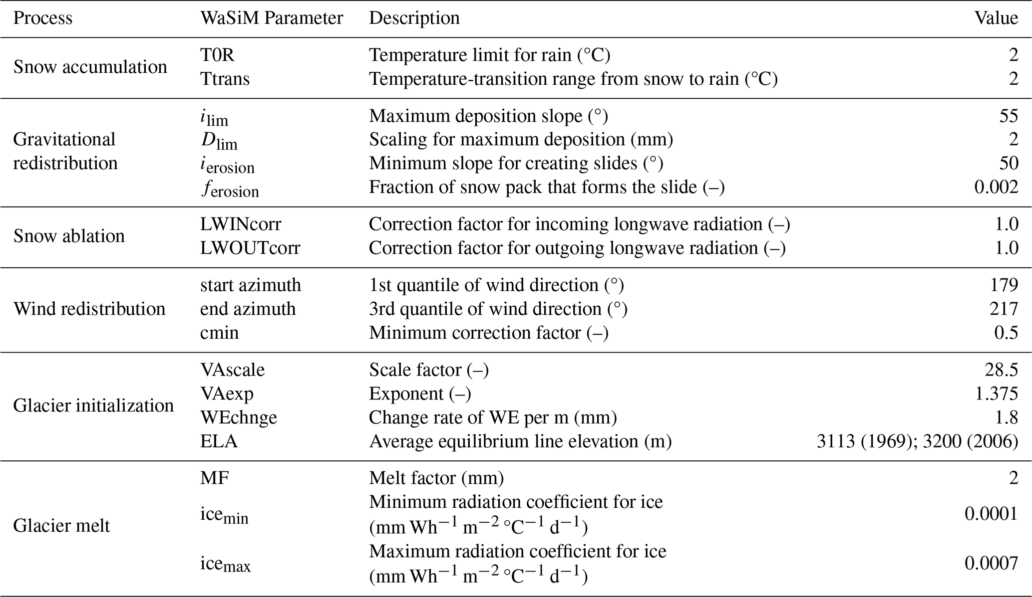
The grid-based Water Flow and Balance Simulation Model (WaSiM) was initially developed for climate and land use change studies in mountainous regions (Schulla, 2021). In previous studies, WaSiM has proven to be a powerful tool for investigating the spatial and temporal variability of hydrological processes in complex river basins (e.g., Strasser et al., 2019). WaSiM uses physics-based modeling approaches to simulate vertical water flux in the unsaturated zone using the Richards equation and an energy-balance approach for snowmelt. Additionally, WaSiM can consider snow redistribution processes induced by wind or gravity, which is highly relevant for high-elevation alpine catchments (Warscher et al., 2013). A detailed explanation of the snow routine can be found in the WaSiM documentation and the publication of Hofmeister et al. (2022). The model parameters for simulating gravitational slides (Table 2) are identical to those of Hofmeister et al. (2022) as the spatial and temporal resolution of the model setup is the same (i.e., hourly time step and 25 m grid resolution). The range of the main wind direction for wind-induced snow redistribution was derived from monthly mean WRF data for the winter period (from October to May). Accordingly, WaSiM corrects snowfall based on exposition, i.e., snowfall from wind-exposed grid cells is moved to sheltered cells. Consequently, the algorithms for simulating wind-induced snow redistribution and gravitational slides are not event-based, as they try to match snow accumulation at the end of the winter. The temperature threshold (T0R) is set to 2 °C, which is in agreement with other studies conducted in the Alpine region (e.g., Frei et al., 2018). The temperature transition range from snow to rain is set to 2 °C (i.e., half snowfall and half rain), allowing a smooth transition between rain and snowfall from 0 °C (i.e., only snowfall) to 4 °C (i.e., only rain). The correction factors for the incoming and outgoing longwave radiation are set to 1, meaning no correction is applied.

A variety of algorithms are available in WaSiM for the interpolation of meteorological inputs. Most of the five input variables (i.e., relative humidity, precipitation, wind speed, and shortwave incoming radiation) are interpolated with a bilinear approach from the 2 km WRF to the 25 m grid resolution of WaSiM. Temperature is inter- and extrapolated based on an elevation-dependent regression approach. The interpolation algorithms are applied at an hourly time step, which allows the consideration of variable temperature lapse rates, which is far more realistic than a fixed temperature lapse rate. For consistency, this approach is identical for uncorrected and corrected WRF temperature. A topography-dependent correction following the approach of Oke (2002) was applied to account for terrain effects on shortwave radiation and air temperature. Incoming shortwave radiation was adjusted according to slope, aspect, and terrain shading through solar-geometry calculations, and air temperature was subsequently modified using an empirical relationship linking local temperature deviations to the radiation correction under prevailing sunshine conditions.

We assume a positive precipitation lapse rate of 0.5 % 100 m⁻¹, which is a common assumption for the Ötztal Alps (Schöber et al., 2014; Schmidt et al., 2022), for re-scaling the relatively coarse WRF precipitation from the 2 km grid resolution to the actual topography of the much finer grid resolution of WaSiM (i.e., 25 m). The 25 m grid resolution of the hydrological model is a compromise between the spatial discretization needed to resolve the small-scale heterogeneity of the research area (∼ 60 km² in size) with complex topography and the computational time required to run the hydrological model at hourly time steps over longer periods (∼ 40 years). With the activated snow redistribution module of WaSiM, preferential snow erosion and deposition are considered and simulated.

Glacier melt and evolution are particularly important for hydrological studies in glaciated catchments such as the upper Kauner Valley. For this, WaSiM offers a dynamical glacier module that adds or removes glaciated grid cells dependent on the specific mass balance (Stahl et al., 2008). The standard threshold value for transforming a grid cell into a glacier cell is 2000 mm SWE. However, WaSiM does not consider the actual ice flow of a glacier. Hence, positive mass gains are not transported from the accumulation to the ablation area of a glacier, which has certain limitations in areas with high glacier dynamics. For initialization, WaSiM estimates the volume of a glacier based on the volume-area scaling (VAS), which offers the main advantage of minimum input data, since glacier extent data are usually available even in data-scarce regions. According to Bahr et al. (2015), the dimensionless exponent of the VAS equation is fixed to 1.375, while the scale factor depends on the sample data set. Since the scale factor can only be estimated for larger sample sizes of around 50 or more glaciers to ensure statistical robustness, an already published scaling factor for the European Alps from Chen and Ohmura (1990) is chosen. Additionally, the dynamic glacier routine in WaSiM enables modeling of snow metamorphism to firn after one balancing period and to ice after six additional balancing periods (hydrological years). The initialization of the firn layer is based on the WEchnge parameter that defines the rate of change in the water equivalent of firn with each meter of elevation increase (default is 1.8 mm m⁻¹) and the average equilibrium line (ELA), which separates the accumulation and ablation area of a glacier. As no continuous ELA information is available for the glaciers of the upper Kauner Valley, we use the ELA in m a.s.l. from a neighboring glacier, the Vernagtferner (WGMS, 2025). Glacier melt is simulated using an extended degree-day approach initially developed by Hock (1999), which includes information on global radiation at each time step and grid cell to modify the ice and firn melt. Besides a classical melt factor (MF), one empirical coefficient for minimum radiation and one for maximum radiation are needed. Hence, glacier melt increases when shortwave radiation input is high and vice versa. Snow melt on the glacier is simulated by the same energy-balance approach as for non-glaciated grid cells to ensure consistency.

In general, we used the standard model parameters from the WaSiM documentation whenever possible (Table 2), as the main focus of this case study is to investigate the sensitivity of WaSiM to changes in forcing data. Although calibrating the main WaSiM parameters can improve model results, we have refrained from parameter optimization to investigate how changes in the forcing propagate to different model results. This means all model parameters are identical for all simulation runs. We use WaSiM version 10.07.02 for all simulations in this study.

Table 2 Key processes and main WaSiM parameters.

3 Results

3.1 WRF temperature at station locations

As a first evaluation, we compare altitude-adjusted uncorrected and corrected WRF temperatures with station observations from the upper Kauner Valley and the surrounding area (Fig. 1 and Table 1). For the comparison of the general statistics of the time series, we use ECDFs, as shown in Fig. 5. The periods of the ECDFs refer to all data since the start of measurement recording (Table 1) until 31 December 2015. No data values in the observations are set to no data in the WRF temperature time series. The lowest station is Dammfuss, at an elevation of 1770 m a.s.l., with continuous temperature records since 1988, followed by the Gepatschalm station, installed at 1900 m a.s.l. in 2009. The second-highest station is Weisssee, at an elevation of 2540 m a.s.l., with continuous temperature observations since December 2006. The station Vernagt Pegel was installed at 2640 m a.s.l. in 1975. Consequently, the selected stations cover an elevation difference of almost 900 m. In addition, the four stations represent four different WRF land use categories (Fig. S2 and Table S1), which are described in the following section.

The four panels of Fig. 5 compare the ECDF of station temperature (black line), of the uncorrected WRF temperature (red line), and the corrected WRF temperature (blue line). We evaluate the similarity between ECDFs using the KS test. The results of the KS tests are listed in Table S4. At Dammfuss, the uncorrected near-surface WRF temperature agrees with the frequency of observed mean and warmer (> 5 °C) temperatures but shows a positive bias (higher frequency) for colder temperatures (Fig. 5a). The frequency distribution of the corrected WRF temperature aligns with the observations at the Dammfuss station and shows only a slight cold bias for temperatures < 0 °C. According to the computed D-statistics (Table S4), the maximum distance between the observed and WRF temperature ECDFs is 0.08 for the uncorrected and 0.03 for the corrected temperature. The maximum vertical difference between the ECDFs is at −3.06 °C in the case of uncorrected and at 17.46 °C for the corrected. The WRF land use category of this particular grid cell is Woodland Mosaic (Fig. S2 and Table S1).

At Gepatschalm station, the critical temperature frequencies are more towards warmer temperatures (> 5 °C) (Fig. 5b). Correcting WRF temperature reduces the warm bias in the range from 5 to 15 °C, but a slight offset remains. Conversely, the cold bias in the near-surface WRF temperature is absent in the corrected time series. The maximum distance between the ECDFs is 0.08 in the case of the uncorrected and 0.07 for the corrected WRF temperature (Table S4). The WRF land use category of this particular grid cell is Evergreen Needleleaf (Fig. S2 and Table S1).

We can also observe a similar cold bias (< 0 °C) between the observation and uncorrected WRF temperature at Weisssee station (Fig. 5c). Using the WRF atmosphere, the cold temperature offset can be corrected, resulting in good agreement with observed temperature records. The maximum distance between the ECDFs is 0.05 in the case of the uncorrected and 0.03 for the corrected WRF temperature (Table S4). The WRF land use category of this particular grid cell is Wooded Tundra (Fig. S2 and Table S1).

The largest cold bias covering the entire temperature range is present at the highest station, the Vernagt Pegel (Fig. 5d). The corrected WRF temperature shows a more realistic representation of temperature frequencies at 2640 m a.s.l. altitude. Therefore, the maximum distance between the ECDFs is much larger (i.e., D-statistics uncorrected 0.13 and corrected 0.03) compared to the lower-elevation stations (Table S4). The respective land cover class of the WRF grid cell is Snow or Ice (Fig. S2 and Table S1).

Although the comparison with the station data only represents specific elevation ranges and locations of the research area, it indicates that the near-surface WRF temperature has difficulties representing the small-scale heterogeneity in surface-albedo characteristics, especially for the higher altitudes (> 2600 m a.s.l.) that are dominated by the Snow or Ice WRF land use category. Hence, the correction approach based on temperature lapse rates from the WRF atmosphere provides more realistic temperature predictions independent of the surface albedo characteristics.

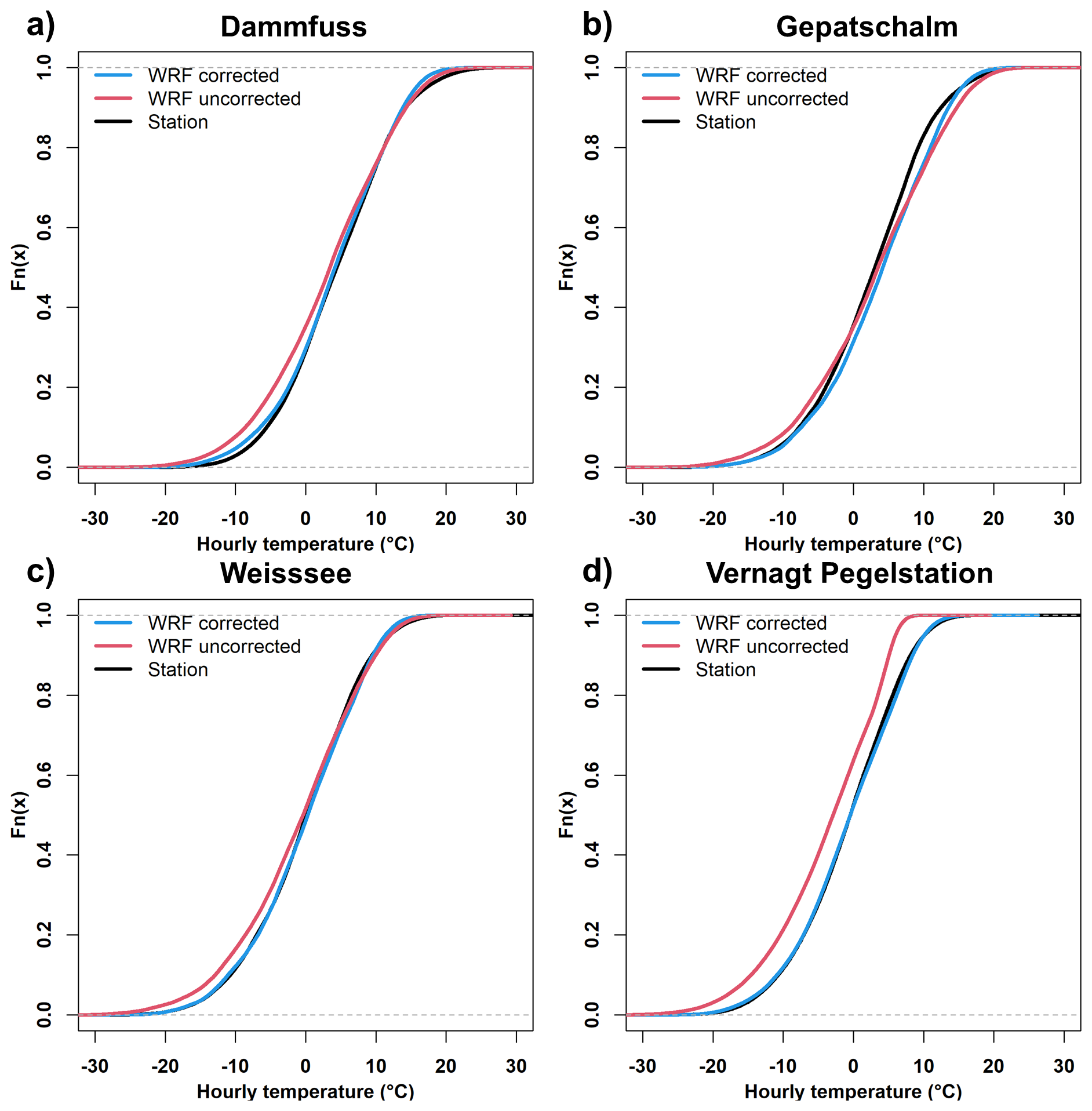
Figure 5 Empirical cumulative distribution functions (ECDF) of observed hourly temperature (black line), uncorrected WRF temperature (red line), and corrected WRF temperature (blue line) at different stations (a) Dammfuss (WRF land use category Woodland Mosaic), (b) Gepatschalm (WRF land use category Evergreen Needleleaf), (c) Weisssee (WRF land use category Wooded Tundra), and (d) Vernagt Pegelstation (WRF land use category Snow or Ice).

In an additional experiment, we assessed the influence of combinations of eta levels on the calculated hourly temperatures at four observation stations (Fig. S10). For this, we calculated TLRs from neighboring eta levels up to eta level 25, as shown in Fig. 4. Interestingly, we observe a larger temperature spread, indicating a greater dependence of the corrected temperature on the eta-level combination at the lower-elevation reference stations (i.e., Dammfuss and Gepatschalm). From the evaluation of goodness-of-fit criteria (Table S3), we conclude that the lowest atmospheric levels (1–2) perform poorly, likely reflecting their stronger sensitivity to local surface and boundary-layer processes. Near-surface temperature gradients can differ substantially from free-atmospheric lapse rates because they are influenced by surface energy exchange and the degree of coupling between the atmospheric boundary layer and the free troposphere (Pepin et al., 2022; Karki et al., 2020). Although individual eta-level combinations yielded slightly better performance at specific stations, the best-performing combinations differed among sites, indicating limited spatial transferability. Therefore, a bulk lapse rate derived from eta levels 1–20 was adopted as a pragmatic compromise between reducing the sensitivity to individual near-surface levels and retaining a coherent representation of the lower-atmospheric temperature gradient. This choice should not be interpreted as a statistically optimized or universally applicable cutoff, but rather as a configuration-dependent choice based on the sensitivity analysis presented here. Because the relationship between eta levels and near-surface temperature gradients depends on the model configuration and local atmospheric conditions, the selected range is not intended to represent a generally transferable threshold. This approach avoids station-specific optimization and provides a consistent framework for temperature extrapolation across catchments with differing topographic and climatic characteristics.

3.2 Robustness of temperature trends and elevation-dependent warming

To evaluate the robustness of the WRF temperature trend, we compare it with a long-term and homogenized observation from the HISTALP data set (Auer et al., 2007). Monthly mean temperature records since 1851 are available at the Obergurgl station, which is approximately 20 km away from the Kauner Valley and located at 1936 m a.s.l. As this site is located in a neighboring valley (i.e., the Ötz Valley), it also serves as a test of the general transferability of the applied correction method for WRF temperatures. The WRF land use category of the respective grid cell is Evergreen Needleleaf. Figure 6a shows the evolution of monthly and annual temperatures at the station Obergurgl. In general, the WRF temperature closely follows the evolution of the observed monthly and annual temperature. The mean temperature at the Obergurgl station is 2.16 °C based on observations from 1973 to 2015. The mean of corrected WRF temperature at the respective elevation (1936 m a.s.l.) is 2.61 °C. Consequently, WRF overestimates the mean temperature by 0.45 °C, as visible in the ECDF plot (Fig. 6b). The mean annual temperature increase is 0.06 °C a⁻¹ at Obergurgl station (Sen's slope of 0.003 °C a⁻¹) and 0.05 °C a⁻¹ for the corrected WRF temperature (Sen's slope of 0.003 °C a⁻¹). Both temperature increases represent a significant positive trend at the 95 % confidence level. The Pettitt test detects a probable change point, meaning a sudden change in the central tendency (i.e., mean), in both time series for May 1987. The sudden warming in the European Alps at the end of the 1980s was already reported by several other studies (e.g., Marty, 2008; Marcolini et al., 2019; Hofmeister et al., 2023). These results clearly show that the bias-corrected RCM data are consistent over a longer period (> 30 years) with respect to non-stationarity. However, we also found that the uncorrected WRF temperature has the identical statistical behavior as the corrected WRF temperature for the Obergurgl WRF grid cell over the same period. Therefore, we did not include the uncorrected WRF time series in Fig. 6.

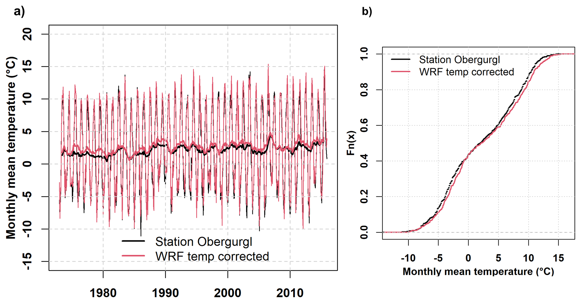
Figure 6 (a) Mean monthly temperature at Obergurgl station (thin black line) and corrected WRF temperature (thin red line) at the respective station altitude. The thicker lines illustrate the respective yearly moving average. (b) ECDF of the respective time series for the same period (i.e., 1973–2015). Note that the uncorrected WRF temperature is not included as it is identical to the corrected WRF temperature for this site, and the lines would overlap.

3.3 Impact of temperature correction on hydrological model results

We use the hydrological model WaSiM to investigate the impact of WRF temperature and relative humidity (RH) corrections at the catchment scale across different hydrological processes, such as snow, glacier, and streamflow generation. The simulation period is from 1 October 2006 until 30 September 2015, but the analysis period is slightly shorter (eight years) as the first simulation year is considered a spin-up period. The multi-data evaluation of the simulation results is limited by the temporal coverage of the WRF data, which is only available until 31 December 2015 in this case study. Hence, the overlap of observed snow depth and snow cover data is relatively short. Nevertheless, the simulation period is long enough to observe similarities and discrepancies between corrected and uncorrected model runs. In the following, T correction refers to simulations forced with bias-corrected WRF temperature, whereas T and RH correction refers to simulations forced with bias-corrected WRF temperature and relative humidity in WaSiM.

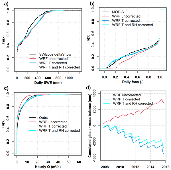
In Fig. 7a, we compare the ECDFs of daily observed SWE at Weisssee station (black line) with simulated SWE at the respective 25 m grid cell of WaSiM. In general, WaSiM tends to overestimate SWE with both corrected and uncorrected model forcing. The simulated SWE appears relatively insensitive to the corrected WRF inputs at this grid cell. The mean daily SWE is 163 mm in the observation, while the simulated SWE with T correction is 187 mm, with T and RH correction 185, and 195 mm in the case of no correction applied. Although comparing in situ SWE with simulated SWE involves several assumptions and uncertainties due to the high spatial heterogeneity of snow processes, the similarity in their behavior offers valuable insights into snow accumulation at 2540 m a.s.l. elevation. We conclude that both correction approaches have little influence on the simulated SWE for this location and elevation.

Figure 7b shows the ECDFs of daily observed and simulated fractional snow-covered area (fsca). Daily observed snow cover data are from MODIS (black line). Not surprisingly, the agreement between observed and simulated fsca is largest during the winter period, when the entire research area is covered by snow (Fig. S12). However, the discrepancy between observation and simulation, as well as between the corrected and uncorrected WRF temperature forcing, increases during the low fsca period. In particular, the simulated fsca with uncorrected WRF temperature input overestimates snow cover in the research area, with values < 0.6 fsca. The ECDF of simulated fsca with corrected WRF temperature is more in line with the fsca of MODIS, especially at low to mid fsca values (i.e., fsca < 0.6). The simulated fsca with T and RH correction (cyan line) has a very similar behavior to the one with T correction (blue line). The negative snow cover bias in both corrected products during the snow-free period (fsca < 0.3) can result from several factors, including snowpack heterogeneity, the limited MODIS sensor resolution, and the fsca processing. Nevertheless, the fsca data cover the entire research area, unlike the in-situ SWE data, and provide valuable information on the seasonal evolution of snow cover. We conclude that both correction approaches yield a more reliable simulation of snow cover, whereas these do not differ significantly from one another, indicating that simulated fsca mainly depends on the temperature correction.

The ECDFs of hourly streamflow at the gauge Gepatschalm are illustrated in Fig. 7c. The observed streamflow (black line) shows a typical behavior for a snow and glacier-dominated catchment with an extended low flow period with a median of 0.85 m³ s⁻¹. The simulated streamflow using uncorrected WRF temperature (red line) significantly underestimates the entire observed ECDF, indicating that WaSiM generates too little streamflow across all seasons (Fig. S13a). The WaSiM runs with T correction (blue line), and the one considering T and RH correction (cyan line) shows a more realistic behavior and follows the ECDF of the observed streamflow. While the mean annual streamflow is well estimated with the T correction (i.e., the mean flow of observation and simulation with T correction are both 3.1 m³ s⁻¹), the T and RH correction simulation run slightly underestimates the mean streamflow (2.89 m³ s⁻¹). For both correction approaches, WaSiM overestimates higher streamflow and underestimates lower streamflow (p< 0.8). Hence, there is potential to optimize WaSiM's seasonal streamflow generation (Fig. S13b and c). We compute goodness-of-fit (GOF) criteria to compare daily observed and simulated streamflow for the respective period. Although WaSiM provides hourly streamflow outputs, we compare daily values because they are expected to be less affected by the fact that WRF does not assimilate precipitation station data from that region, which limits direct hourly comparisons. For daily values, we assume that model performance depends more on the accurate prediction of snow and glacier dynamics than on intense precipitation events. The daily GOF criteria with uncorrected WRF temperature are KGE 0.42, percent bias −46, and RMSE 2.5 m³ s⁻¹. The daily performance with T correction is much better with KGE 0.71, percent bias −0.7, and RMSE 2.4 m³ s⁻¹. Despite the underestimate of the mean streamflow by −6.9 %, the other two performance indices (i.e., KGE 0.78; RMSE 2.14 m³ s⁻¹) enhanced when considering T and RH correction in WaSiM. The improvement in model performance is due to lower overestimation of streamflow peaks during the summer period (Fig. S13b and c), resulting from reduced glacier melt contribution. We observe no changes between the two correction products during the low-flow period (Fig. S13b and c). Accordingly, we conclude that the major improvement in streamflow prediction originates from the temperature correction. Nevertheless, the sequential thermodynamically consistent correction of WRF relative humidity further enhances WaSiM's performance in runoff generation during the glacier melt period. It is worth noting that the only differences between the WaSiM simulations are the WRF bias corrections applied. We did not apply a calibration strategy (i.e., manual or auto calibration) to optimize the model parameters based on the model forcing. This shows the importance of the correct meteorological forcings for model parameterization, including physics-based models, to achieve high model performance.

The simulated cumulated glacier mass balances indicate the highest sensitivity concerning the temperature forcing (Fig. 7d). The cold bias in near-surface WRF temperature (red line) results in a constant positive glacier mass balance, which is quite unrealistic for the period 2008 to 2015. In the highest parts of the research area (> 2700 m), the cold bias results in too low snowmelt and, hence, an overestimation of the snow cover (Fig. 7b). As long as the glaciers are snow-covered and not exposed to incoming radiation, WaSiM does not compute melt from firn and ice. When forcing WaSiM with the T correction (blue line), as well as with the T and RH correction (cyan line), the simulated glacier mass balances exhibit stronger seasonality and a continuous negative trend, which are more in line with the observed annual mass balances of the nearby Kesselwand glacier (Fig. S16). The Gepatsch and Kesselwand glaciers share parts of the accumulation area. The only exception in the negative trend is the winter period of 2013/14, which was particularly snowy, and the following summer was cooler and wetter. The mass balance for the 2013/14 year was nearly balanced in the Central European Alps, with only a slight negative average balance of −174 mm (WGMS, 2017). An additional comparison of simulated glacier mass balances with observed geodetic elevation changes (Sect. S2.6) strengthens the WaSiM's ability to reliably predict glacier dynamics, especially when forced with the T and RH correction (Fig. S14). At the end of the simulation period, we observe a deficit of almost 6000 mm in the catchment water balance when comparing the uncorrected and T-corrected simulation runs (Fig. 7d). As snow and glacier melt are the dominant streamflow components in the upper Kauner Valley during this period, the deficit in meltwater directly propagates into streamflow generation (Fig. S13a–c).

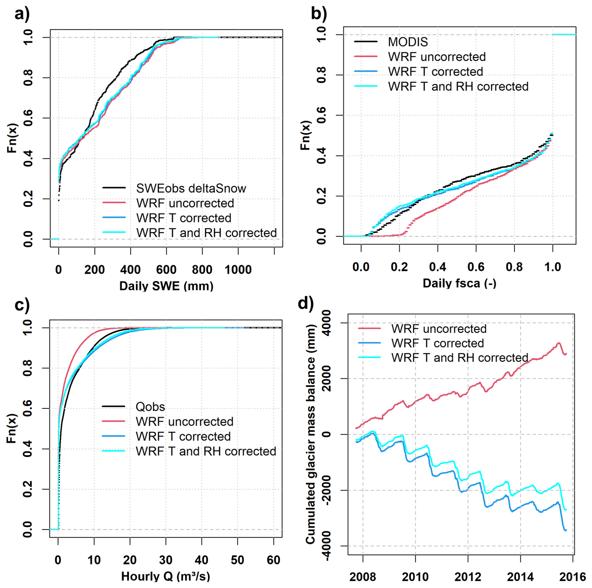
Figure 7 Empirical cumulative distribution functions of observed (black line) and simulated (a) SWE at station Weisssee, (b) fractional snow covered area (fsca), (c) streamflow at gauge Gepatschalm, as well as (d) simulated glacier mass balances averaged over the catchment. Simulation results with uncorrected WRF temperature (red line), corrected WRF temperature (blue line), and corrected temperature and RH (cyan line).

Table S5 summarizes the main water balance components simulated with the uncorrected WRF temperatures and the two corrected products. Since the only difference in the model forcing is the temperature and relative humidity input, the total precipitation is identical in all three model runs. The mean annual precipitation sum for the period 2008–2015 is 1487 mm. Due to the cold bias in the uncorrected WRF temperature, the mean snowfall fraction of total precipitation is slightly higher (68 %) than that of the corrected simulation runs (62 %). Consequently, the fraction of rain in precipitation is smaller for the simulation run with uncorrected WRF temperature. Despite interannual variability in streamflow magnitudes, the mean annual streamflow sum simulated with T correction matches observations quite well, with only a slight underestimation of < 1 %. The simulation run with T and RH correction underestimates the observed annual streamflow sum by about 7 %. The simulated streamflow with the uncorrected WRF temperature underestimates annual streamflow by almost 50 % (Fig. S13a). The highest mean annual evapotranspiration is obtained with T and RH correction (i.e., 84 mm), as a drier atmosphere leads to a higher vapor pressure gradient. The evapotranspiration with only T correction is about 19 % smaller (i.e., 68 mm), and even smaller in the case of uncorrected WRF forcing with a mean evapotranspiration of 62 mm. We additionally evaluate the simulated sublimation rates on glaciated cells. The uncorrected WRF temperature yielded the lowest mean annual sublimation with 8.39 mm. In the case of corrected WRF temperature, 12.8 mm mean sublimation was simulated, and 20.5 mm sublimation when corrected WRF temperature and relative humidity were considered as model forcing.

Based on these facts, we can assume that the critical aspect of the simulation results with uncorrected WRF temperature is not the amount of snowfall or evapotranspiration, but rather the timing and magnitude of simulated snowmelt, which requires positive temperatures, especially in higher-elevation parts of the catchment. While covered with snow, WaSiM does not compute firn and ice melt on glaciated cells, leading to a significant discrepancy in the simulated glacier mass balances, as shown in Fig. 7d and the calculated mean glacier mass balances in Table S5. From the model results, we conclude that the temperature correction is essential for reliable prediction of seasonal snow and glacier processes and, consequently, for streamflow generation. Nevertheless, the sequential thermodynamically consistent correction (i.e., T and RH correction) further enhances the magnitude of seasonal streamflow, especially in August and September, when glacier melt contributes most.

3.4 Longer simulation run (1973–2015)

Given the relatively short simulation period of eight years, the near-surface uncorrected WRF temperature does not yield plausible hydrological model results, especially for snow and glacier processes (Fig. 7). On the contrary, using TLRs from the WRF atmosphere results in reliable model predictions for several processes, including snow and glacier melt and streamflow generation. Considering WRF T and RH correction yields the best model performance for simulated streamflow. In this section, we test the robustness and consistency of the hydrological model results with the two corrected WRF products over a 42-year simulation period. We initialized WaSiM in 1969 using glacier extents from 1968 and considered a spin-up period of three years, so the actual analysis period began in 1973.

As almost continuous observed streamflow data have been available at gauge Gepatschalm since 1971, we compare hourly and daily streamflow over different periods in the Supplement (Sect. S2.5 and Fig. S15). WaSiM reproduces the observed seasonal streamflow pattern well, including the shift in runoff timing and the increase in summer discharge in later periods, but it tends to underestimate low flows and overestimate late-summer flows. Overall performance is strong despite the model not being explicitly calibrated to the different model inputs. The model run that considers T and RH correction yields slightly better KGE (0.8) and RMSE (2.2 m³ s⁻¹), while the one with the T correction has a smaller percent bias (−5.5).

The evolution of annual mean temperature and the consequences for snow and glacier development are presented in Fig. 8. The first panel of Fig. 8 shows the corrected mean annual WRF temperature evolution of the research area. The vertical red line represents a significant change point in the annual temperature time series detected by the Pettitt test in 1987. This particular change point has already been observed in previous studies in different parts of the European Alps (e.g., Marty, 2008; Marcolini et al., 2019; Hofmeister et al., 2023).

Both simulated glacier mass balances (i.e., with T correction in blue; with T and RH correction in cyan) exhibit a continuous negative trend from the end of the 1980s (Fig. 8b). Before that, the glaciers were in equilibrium or even had slight positive mass balances. The positive glacier mass balances align with observed advances of Gepatsch- and Weissseeferner (Altmann et al., 2020), as well as the observed mass balances of the nearby Kesselwand glacier (Fig. S16). As the graph shows hourly simulation results, the seasonal variability of snow accumulation and ice ablation is clearly visible in periods with negative glacier mass balance. In general, the simulation run with T and RH correction yields less negative mass balances than the simulation run that considers only temperature correction. Consequently, the Pettitt test detected a significant change point earlier (i.e., 1994) than for the model run with T and RH correction (i.e., 2001). An additional evaluation of the simulated glacier mass balances against observed glacier mass changes from an elevation change product (Hugonnet et al., 2021) revealed an overestimation of cumulated melt rates at the end of the simulation period in 2015 by 36 % in the case of T correction and by 22 % in the case of T and RH correction.

The simulated fractional glacier cover (fglc) shows a high similarity between the two corrected methods (Fig. 8c). Mainly during the periods of glacier growth around the 1980s and the strong recession from the late 1990s, differences can be observed. Both correction products lead to a significant change point in the fractional glacier cover (fglc) in 2000. In general, the evolution of the simulated fglc shows a pattern similar to that of the cumulative glacier mass balances. The black triangles illustrate years with observation data. Both simulated fglc follow the negative trend of the observations but have a positive offset at the end of the simulation period (i.e., observed fglc is 0.3, simulated with T correction is 0.35, and with T and RH correction is 0.37).

Figure 8d represents the long-term evolution of simulated snow cover duration (scd) forced with the two corrected products, which show an almost identical mean scd. The Pettitt test found a significant change point in 1985 for both simulation runs. Before 1985, the mean scd was fluctuating between 290 and 330 d. After 1985, scd never exceeded 310 d and was even below 260 d in 2002. The significant reduction in scd is a prerequisite for negative glacier mass balances, as more firn and ice are exposed to the shortwave radiation for a longer period, leading to higher melt rates. As high elevation (> 2700 m a.s.l.) and glaciated areas, which are mainly or permanently covered by snow, the sensitivity of mean scd is rather small. Consequently, we conclude from long simulation runs that the sequential, thermodynamically consistent correction of WRF relative humidity further enhances simulated glacier mass balances and the magnitude of summer streamflow, especially in August and September.

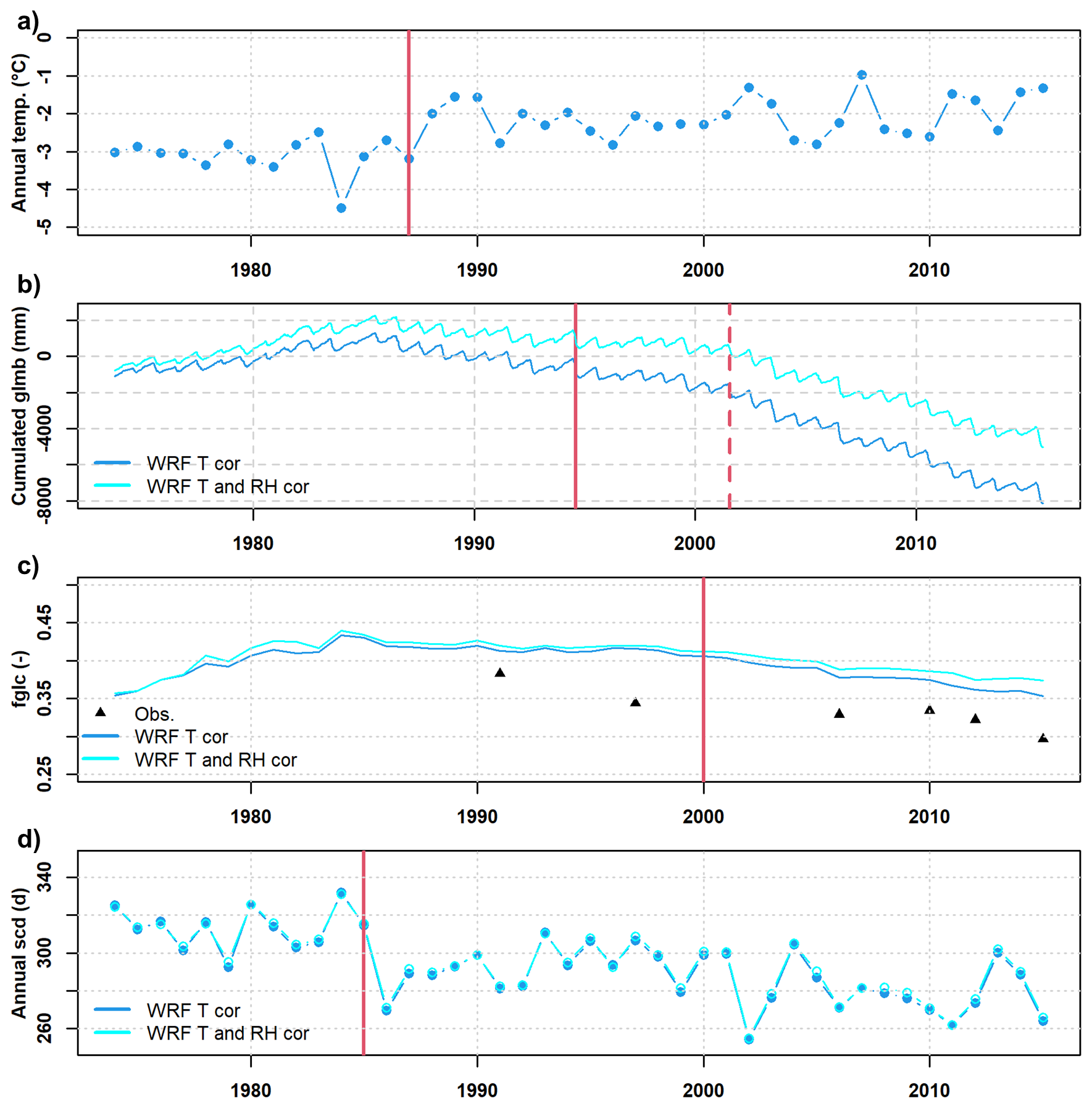
Figure 8 Catchment averages of (a) simulated mean annual temperature, (b) simulated cumulated glacier mass balances (glmb) with T correction (blue line) and T and RH correction (cyan line), (c) observed (black triangles) and simulated fractional glacier cover (fglc) with T correction (blue line) and T and RH correction (cyan line), and (d) simulated annual snow cover duration (d) with T correction (blue line) and T and RH correction (cyan line). Significant change points are indicated with a vertical dashed red line in the case of the T and RH corrected simulation run, and as a red solid line for the T corrected simulation run. Different change points are only detected for (b) simulated glmb. For the other variables, the change points are identical. The years represent hydrological years (i.e., 1 October to 30 September).

4 Discussion

4.1 Physical consistency among meteorological variables

The temperature correction based on hourly TLRs, derived directly from the WRF atmosphere using spatially averaged temperature and geopotential height fields at the model eta levels, has been shown to be a robust alternative to the commonly used univariate empirical quantile mapping, which strongly depends on the quality and availability of temperature observations and requires nonstationarity conditions. The WRF temperature correction based on TLRs had a significant impact on the hydrological model results, which is not surprising as the main processes in high-elevation catchments (i.e., snow and glacier dynamics) depend highly on a reliable spatiotemporal temperature distribution (Meyer et al., 2019). It should be mentioned at this point that the temperature extrapolation from two different vertical WRF representations (i.e., eta level 1 in Eq. 4 and WRF 2 m temperature in Eq. 6) is not strictly physically consistent. However, the objective is to compare these to different WRF near-surface representations against station observations, after elevation normalization, to decompose the temperature bias and evaluate complex-terrain temperature behavior.

In addition, the hydrological model results across different simulation periods further underscore the need for a sequential thermodynamically consistent correction of relative humidity in physics-based simulations of seasonal cryohydrological processes. Empirical bias correction methods that preserve absolute moisture and account for temperature-dependent saturation, such as the August-Roche-Magnus formula (Sect. S2.1), have been shown to account for nonlinearity in the elevation dependency of the cold bias in the WRF data (Fig. S4). Due to the correction of hourly relative humidity data, even sub-daily cycles in temperature and relative humidity are considered when correcting WRF T and RH. Ignoring the thermodynamic correction for relative humidity breaks the physical links between temperature and relative humidity, affecting energy-balance calculation and evaporation estimates in the hydrological model (Meyer et al., 2019). The uncertainty in the sequential thermodynamically consistent correction of relative humidity can be reduced by directly using the specific humidity and dew point temperature of WRF. However, these output variables were not stored and are therefore unavailable for further analysis and testing.

We have not applied a bi- (i.e., considering temperature and relative humidity simultaneously) or multivariate bias correction, including WRF precipitation. However, multivariate bias corrections require higher computational resources and are methodologically complex. In addition, the demand for sufficiently long, high-quality observations across all variables to estimate joint distributions increases significantly (Meyer et al., 2019).

Another important meteorological variable is incoming shortwave radiation, which the WaSiM model empirically corrected for terrain effects and day of the year. However, we have not evaluated the topography-dependent corrections for solar radiation. In our case study, WRF wind speed was generated at 10 m above ground and was not adjusted to the finer topography of the WaSiM model. Since dynamical downscaling of wind speed and direction requires a complex model approach (e.g., Wagenbrenner et al., 2016; Quéno et al., 2024), we have refrained from doing so, given that wind speed does not influence snow redistribution in WaSiM. Wind speed primarily influences snowmelt and evapotranspiration rates in WaSiM. Since WaSiM considers only a single dominant wind direction for wind-induced snow redistribution, time-dependent forcing using actual wind directions is not yet possible.

4.2 Representation and evolution of land use categories in WRF

Besides the spatial representation of land cover properties and topography in high-resolution RCMs, another question is whether the long-term evolution of surface properties is considered. Due to the increasing greening effect (i.e., increase in vegetation productivity) and the fast retreat of glacier cover in the proglacial areas (Rumpf et al., 2022), constant land cover classes cannot account for the accelerated change of the surface-albedo properties in high-elevation catchments. Especially for long-term (> 30 years) climate-related studies, a constant land cover parameterization may lead to implausible behavior of important meteorological variables (e.g., temperature) that are particularly sensitive to surface albedo. This behavior will impact all following analyses, as demonstrated in this case study. Hence, there is a need for either a robust workaround, as introduced in this technical note, or the representation of a dynamic land cover. The latter is particularly problematic, as land cover information for the Alpine region, for example, is scarce before 1950 due to the lack of remote sensing data, and reconstructing earlier stages is particularly complex (Ramskogler, 2023). Additionally, the re-initialization with updated land cover is a complex task and can lead to unrealistic behavior in RCM and hydrological model simulations. Hence, a robust workaround might be the most suitable approach for many longer-term RCM applications in snow- and glacier-dominated areas.

4.3 Uncertainties in the model cascade

Uncertainties affect all parts of the complex model cascade used in this case study (Jobst et al., 2018; Meyer et al., 2019). The widely used global atmospheric reanalysis product (20CRv3) only assimilates surface pressure data that ensures temporal homogeneity over the entire reanalysis period (i.e., 1836–present), but the limited input data strongly influence variables such as precipitation or near-surface temperature, as they are not directly constrained by observations (Slivinski et al., 2019). Although the ERA5 reanalysis dataset is widely used in Europe for climate change impact studies, it is limited for long-term cryohydrological studies, particularly for the LIA in 1850, since ERA5 data are available only from 1940.

Another source of uncertainty is the parametrization and handling of the boundary conditions of the WRF model. To reduce uncertainty in dynamical downscaling from the global reanalysis product (20CRv3) to WRF, a nested approach was adopted that uses three spatial domains and resolutions (18, 6, and 2 km). Although the 2 km WRF can resolve convection and orographical effects in the central European Alps, the resolution is still too coarse to plausibly represent temperature and precipitation patterns in high-elevation catchments. As demonstrated in this case study, considerable implausible behavior originates from the direct use of the 2 km WRF data as model forcing for a high-resolution (i.e., 25 m) hydrological model. Based on this observation, we conclude that space-related uncertainty (including elevation gradients) between WRF and WaSiM is the dominant source of uncertainty in the applied model cascade. One plausible argument is that a statistical bias correction would remove the cold bias in the diagnosed 2 m WRF temperature. However, this requires long-term and continuous temperature observations at higher altitudes (> 2700 m), which are particularly scarce and provide only in-situ information. In addition, meteorological observations are highly affected by errors and failures at these altitudes (Hofmeister et al., 2023). In fact, higher elevations in mountainous regions have experienced stronger warming trends (e.g., Rangwala and Miller, 2012; Kuhn and Olefs, 2020), as is also evident in the WRF temperature data (Table S6), which challenges the linear extrapolation of statistical bias corrections to higher elevations.

We have refrained from a comprehensive calibration of the hydrological model parameters, as our intention was to demonstrate the impact of WRF bias corrections on the hydrological model results. Although we observed elevation differences between WRF and the stations of more than 500 m in some locations of the domain (e.g., Dammfuss), which probably causes a bias in longwave radiation due to increased scattering through the atmosphere, we have not calibrated the incoming and outgoing longwave radiation of WaSiM, as this would be outside the scope of this technical note. Hence, we used a standard parameterization that relied mainly on values from the literature. Usually, parameter optimization algorithms try to compensate for errors in the model forcing (Meyer et al., 2019) by selecting extreme and implausible values within the parameter ranges (e.g., for the rain-snow threshold), especially when applied in a single-objective calibration. A multi-objective optimization approach will most likely fail to provide reasonable and plausible model results for individual processes, such as snow and glacier dynamics and their interactions with streamflow generation (van Tiel et al., 2022; Schaffhauser et al., 2024; Meyer et al., 2019) under the assumption of biased model forcing.

Another major uncertainty in the hydrological model setup concerns the initialization of the glacier volume, especially in highly glaciated catchments such as the upper Kauner Valley. Due to a lack of glacier data in 1968, we had to rely on published values to parameterize the VA scaling factor (Chen and Ohmura, 1990). Another uncertainty arises from the conceptual glacier routine implemented in WaSiM, which does not account for actual ice flow dynamics when balancing mass between accumulation and ablation areas. This is particularly problematic when the model is applied for longer simulation periods, as demonstrated by Pesci et al. (2023). We observed a delayed recession in the simulated fractional glacier cover (Fig. 8c), which is most likely an effect of the simple glacier representation in WaSiM. In general, it is well known that simplified glacier routines have issues when applied for periods with positive glacier mass balances and glacier advance (Seibert et al., 2018; Schaffhauser et al., 2024).

The date and length of the initialization period slightly impact the simulated annual streamflow. When starting WaSiM in 1969, the annual streamflow was 1.1 % lower at the end of the simulation period compared to the simulation that started in 2006 in the case of the T correction model run. Together with the consistent GOF criteria, this indicates that WaSiM forced with bias-corrected WRF provides reliable results over a simulation period of 42 years. Consequently, these results show that the hydrological model provides essential information on the performance and reliability of downscaled and bias-corrected meteorological reanalysis data for high mountain areas. Process-based evaluation of hydrological model results provides comprehensive information on the quality of bias correction methods and should therefore be an integral part of bias correction frameworks for RCMs (Meyer et al., 2019).

5 Conclusions

This technical note presents a physically based post-processing workflow for correcting coarse-resolution (2 km) regional climate model output for high-resolution (25 m) hydrological simulations in high-elevation, glacierized catchments. Evaluation of WRF output in the upper Kauner Valley revealed a pronounced cold bias in the diagnosed 2 m temperature at the highest stations (> 2600 m a.s.l.), which was linked to the coarse representation of snow and glacier cover and its influence on land-atmosphere interactions. Because observational data at very high elevations are sparse and often non-stationary, commonly applied empirical bias-correction methods such as quantile mapping are of limited suitability for process-based hydrological modeling in snow- and glacier-dominated environments.

To address this limitation, we developed a method that derives hourly temperature lapse rates directly from the WRF atmosphere using spatially averaged temperature and geopotential height fields at the model eta levels. This approach minimizes the influence of surface-related biases and enables the reconstruction of near-surface temperatures from the first atmospheric model level. In addition, relative humidity was corrected sequentially using the corrected temperature to ensure thermodynamic consistency at hourly time scales.

The corrected temperature product showed substantially improved agreement with observations across an elevation gradient of nearly 900 m and led to significantly improved simulations of cryospheric and hydrological processes when used to force the WaSiM model. In contrast, simulations driven by uncorrected WRF data failed to reproduce key characteristics of snow accumulation and melt, glacier mass balance, snow cover dynamics, and streamflow. Among all correction steps, the temperature correction had the largest impact on model performance, highlighting the critical role of an accurate spatiotemporal temperature field in high-mountain catchments. The thermodynamically consistent correction of relative humidity further improved the magnitude of late-summer streamflow during periods of maximum glacier melt.

Comparison with homogenized long-term station observations demonstrated that the corrected WRF temperatures preserve the observed warming signal over the period 1973–2015, indicating that the method is suitable for climate impact assessments. The similarity of long-term trends in corrected and uncorrected WRF temperatures outside snow- and ice-dominated areas further supports the conclusion that the primary bias originates from the representation of surface conditions rather than from the free atmosphere.

Overall, the proposed workflow provides a transferable and physically consistent alternative to empirical bias-correction methods for high-elevation environments. By reducing biases associated with coarse land-cover representations while preserving long-term climate signals, this approach improves the suitability of regional climate model output for hydrological and cryospheric impact studies in glacierized mountain catchments. Future work should evaluate the applicability of the approach in catchments with different climatic and topographic settings and investigate the influence of spatial averaging on lapse-rate estimation at larger spatial scales.