Investigating terrestrial water storage change in a western Canadian river basin with GRACE/GRACE-FO and fully-integrated groundwater – surface water modelling

As hydrological trends shift in response to a warming climate, accurate characterization of hydrologic conditions and hydrologic change are imperative for water resources management, which is particularly important in the Canadian Prairies. In the study herein, a HydroGeoSphere (HGS) fully integrated groundwater – surface water (GW-SW) model is employed to evaluate trends and drivers of surface and subsurface water storage changes in the South Saskatchewan River Basin (SSRB). Terrestrial water storage anomalies (TWSA) derived from the Gravity Recovery and Climate Experiment (GRACE/GRACE-FO) are compared to HGS results; strong correlation is identified. The HGS model allows for the analysis of the constituent water storage components of TWSA, namely surface water, soil moisture, and groundwater, and the GRACE/GRACE-FO solutions are used to validate the regional-scale TWSA and the interannual trends present in the SSRB TWSA time series. Meteorological and oceanic drivers and their impact on interannual hydrological trends in the SSRB are examined. Time-frequency analysis reveals a harmonic trend present in the SSRB TWSA with a period of 2.7–3.0 years, the inverse of which is present in the Oceanic Niño Index. The largest intra-annual water storage fluctuation is found in the soil profile, followed by snowpack, while groundwater experiences longer, multi-year cyclicity. Warm oceanic conditions align with dry conditions and less snowpack in the SSRB, which leads to negative TWSA anomalies. Incorporating both high-resolution GW-SW models and regional-scale satellite gravimetry-derived estimates of TWSA facilitates a comprehensive analysis of hydrological dynamics in the Canadian Prairies and improved characterization of surface water and groundwater storage changes.

1 Introduction

The Canadian Prairies are home to diverse grasslands, wetlands, boreal forest, and extensive agriculture, and contain over 80 % of Canada's arable land (Veeman and Veeman, 2015). Climate change threatens to increase the likelihood and severity of extreme weather events and the gradual increase in average temperature is predicted to lead to increased evapotranspiration and rainfall and reduced snowpack throughout the prairie ecozone (Bonsal et al., 2013; Sauchyn et al., 2020; Tanzeeba and Gan, 2012). These changes to the hydrological dynamics of the Canadian Prairies will impact ecosystems and the sustainable management of water for urban, industry, and agriculture use (Wheater and Gober, 2013). As changing meteorological conditions impart demonstrable impact to water resources, the ability to model the complex interactions between different terrestrial water storage reservoirs (i.e., the land surface, soil profile, and groundwater system) becomes increasingly important. Further developing an accurate understanding and characterization of short- and long-term trends in regional hydrology is essential for preparing for the effects of climate change (Armour et al., 2013; Masson-Delmotte et al., 2021).

This study considers four integrated components of terrestrial water storage, namely surface water (e.g., rivers, lakes, and streams), soil moisture (i.e., water content in the unsaturated zone), groundwater (i.e., water content in the fully saturated zone), and snowpack. Increasingly it is recognized that there is significant interaction between these components, and considering the exchange between components is critical for comprehensive representation of a terrestrial water system (Barthel and Banzhaf, 2016). Isotopic mass balance methods and deterministic modelling have been used to confirm and quantify interactions between terrestrial water storage components (Barthel et al., 2008; Hwang et al., 2018, 2023) which become even more important to consider in the context of climate change as impacts to individual components, such as reduced snowpack, can have cascading effects on terrestrial water storage in a given region (Hayashi and Farrow, 2014). This study facilitates a comprehensive assessment of terrestrial water storage in the Canadian Prairies by combining integrated model-based and independent satellite gravimetry-based estimates of terrestrial water storage changes.

Terrestrial water storage in the Canadian Prairies is impacted by large-scale meteorological and atmospheric anomalies (e.g., the El Niño Southern Oscillation (ENSO)) through temperature and precipitation anomalies that impact evapotranspiration and infiltration rates (Garnett and Khandekar, 2015; Knox and Lawford, 1990; Shabbar et al., 2011). Many global-scale pressure and temperature anomalies fluctuate with multi-year cyclicity that is not necessarily resolvable at short time scales. In addition, climate change is impacting the behaviour of these large-scale meteorological patterns, including the increased frequency of multi-year ENSO events (Lu et al., 2025). Thus, examining the time-variable frequency content of terrestrial water storage alongside indices representing global atmospheric and oceanic anomalies allows for the assessment of drivers of water storage change in the Canadian Prairies, which can lead to better predictive capacity for water management purposes. While relationships between these indices and individual components of terrestrial water storage (e.g., streamflow) have been assessed (Asong et al., 2018; Garnett and Khandekar, 2015; Knox and Lawford, 1990; Shabbar et al., 2011; Shabbar and Bonsal, 2004; Shabbar and Skinner, 2004), this study provides a more comprehensive evaluation linking large-scale atmospheric fluctuations with all components of terrestrial water storage in the Canadian Prairies.

The Gravity Recovery and Climate Experiment (GRACE, 2002–2017) and its follow-on mission (GRACE-FO, 2018 to present) have been used extensively to examine hydrological dynamics (Chen et al., 2009; Crowley et al., 2008; Tapley et al., 2019). GRACE/GRACE-FO provides near-uniform global spatial coverage which is unavailable via in-situ observations and is especially challenging to obtain in remote and sparsely inhabited regions. GRACE/GRACE-FO measurements are used to derive a monthly, vertically integrated (i.e., snow water equivalent, surface water, soil moisture, and groundwater) terrestrial water storage anomaly (TWSA). Observations from GRACE/GRACE-FO have been used to study event-scale drought and flooding (Abelen et al., 2015; Girotto et al., 2017; Scanlon et al., 2021) and long-term hydrological trends (Fatolazadeh and Goïta, 2021; Humphrey et al., 2016; Scanlon et al., 2018). Hydrological model outputs are used in conjunction with GRACE/GRACE-FO to isolate particular components of terrestrial water storage such as groundwater (Famiglietti et al., 2011), or to examine drivers of terrestrial water storage change, such as irrigation (Scanlon et al., 2021). Hamdi et al. (2025) combines GRACE/GRACE-FO data with remotely sensed precipitation, evapotranspiration, soil moisture, runoff, and snow thickness, using a machine learning approach to estimate groundwater storage in the Saskatchewan River Basin. At the scale of the SSRB, GRACE/GRACE-FO can sufficiently (< 2 cm equivalent water height (EWH) error (Vishwakarma et al., 2018)) resolve TWSA changes and is independent of hydrological models used herein, making it a useful tool for comparison and validation.

This study employs a HydroGeoSphere (HGS; Aquanty, 2024) fully integrated groundwater – surface water (GW-SW) model. HGS simulates surface and subsurface flow using a modified form of the Richards' equation for variably saturated flow, the diffusion wave equation for depth-integrated surface flow, and the Manning's equation for open channel flow. HGS has been used extensively in Canadian hydrological analyses, including in the Athabasca River Basin north of the SSRB (Hwang et al., 2023) and the Northern Great Plains (Frey et al., 2021). In a region with complex and variable hydrological dynamics including the prairie pothole region, the fully integrated HGS model is well suited to represent all components of terrestrial water storage (Barthel et al., 2008; Barthel and Banzhaf, 2016).

To examine water storage variability in the SSRB, the HGS model output is used in conjunction with estimates of TWSA derived from GRACE/GRACE-FO. Additionally, TWSA data from a global hydrological model, namely the Global Land Data Assimilation System (GLDAS) Catchment Land Surface Model (CLSM; Li et al., 2020; Rodell et al., 2004), is included for comparison. Combining hydrologic model-based estimates of water storage anomalies with dedicated satellite gravity observations allows for the independent validation of model results, and the HGS model allows for the analysis of individual storage components in the SSRB, including surface water, soil moisture, and groundwater.

The main objectives of this study are to (i) compare satellite gravimetry-derived terrestrial water storage anomalies with hydrologic model-derived terrestrial water storage anomalies in the SSRB over a period of 17 years, (ii) separate the satellite gravity-derived TWSA into water storage components using the model-derived TWSA and assess the time-variable frequency content of each water storage component, and (iii) assess climatological drivers of hydrologic trends in the SSRB based on a time-frequency analysis of the TWSA.

Section 1.1 provides an overview of the study area. Section 2 provides a detailed description of the data and pre-processing steps used in the analysis and is followed by the presentation and discussion of study results in Sect. 3. Section 4 provides key conclusions and an outlook for future work.

1.1 Study Area

The South Saskatchewan River Basin (SSRB) spans from the eastern slopes of the Rocky Mountains to the confluence of the North and South Saskatchewan Rivers in central Saskatchewan and covers roughly 17 % of the land area in Alberta. The land surface elevation ranges from approximately 580 to 3510 m (CVGD2013). The basin is characterized by a semi-arid cold continental climate, with a large variation in temperature throughout the year (40 to − 40 °C). The percentage of surface water usage that is attributed to agricultural use is 9 % on average across Canada, but in the SSRB, agriculture accounts for 85 % of all surface water usage (Martz et al., 2007). Reliance on groundwater is widespread especially among rural residences, and demand for groundwater could increase if a warming climate affects surface water availability (Sauchyn et al., 2020; Wheater and Gober, 2013). This study focuses on the portion of the SSRB located primarily within the province of Alberta, Canada (see the study region outlined in Fig. 1), including the Bow River Basin, the Red Deer River Basin, the Lower Saskatchewan River Basin, and the Oldman River Basin. Though the study excludes the Saskatchewan portion of the SSRB, the study area will be referred to as the SSRB for brevity.

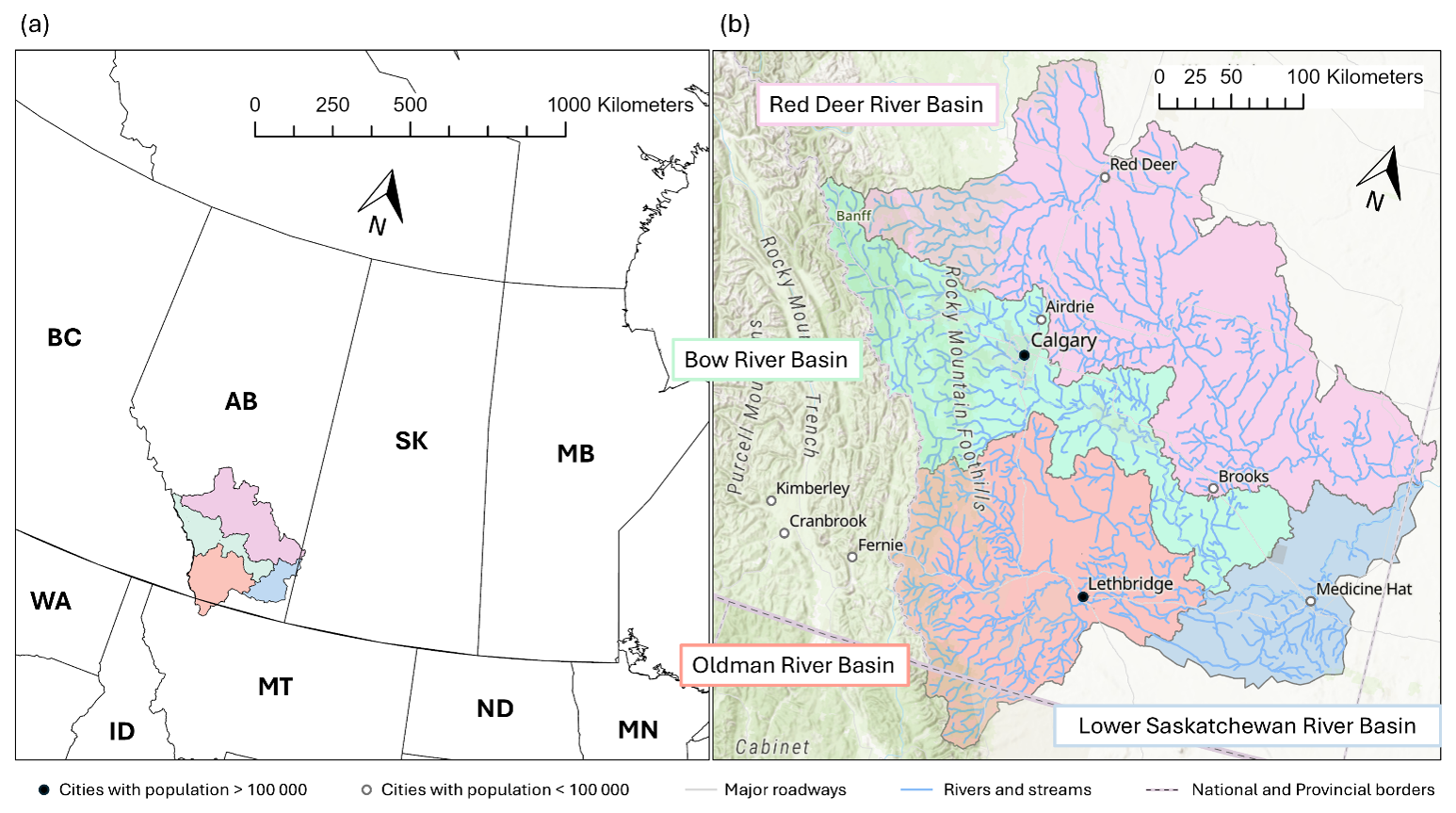
Figure 1 (a) Map of Canada and the United States showing the Alberta portion of the South Saskatchewan River Basin, with provinces and states labelled (British Columbia (BC), Alberta (AB), Saskatchewan (SK), Manitoba (MB), Washington (WA), Idaho (ID), Montana (MT), North Dakota (ND), and Minnesota (MN)). (b) Map of the Alberta portion of the South Saskatchewan River Basin and its major subbasins with major roadways, population centres, and rivers and streams. Bow River Basin (green), Oldman River Basin (orange), Red Deer River Basin (pink), and the Lower Saskatchewan River Basin (blue).

The headwaters of the South Saskatchewan River originate on the eastern slopes of the Rocky Mountain foothills which form the western boundary of the SSRB. Snowmelt from the Rocky Mountains accounts for much of the surface water flow in the SSRB, including approximately 80 % of the streamflow of the Bow River, which in turn makes up around 43 % of the annual flow of the South Saskatchewan River (Ghoreishi et al., 2021). The Bow, Oldman, and Red Deer Rivers all originate in the Rocky Mountain foothills, while the South Saskatchewan River begins at the confluence of the Bow and Oldman Rivers between Lethbridge and Medicine Hat, and is eventually joined by the Red Deer River near the Alberta/Saskatchewan border. The western portion of the SSRB falls within the Montane Cordillera ecozone, where annual precipitation ranges from 500 to 800 mm annually (Natural Resources Canada, 2010; Wilken et al., 1996). This portion of the SSRB contains significant temperate and sub-polar needleleaf forest which transitions into shrubland in the eastern direction. Temperatures in the SSRB vary with altitude but generally range from − 30 to + 30 °C annually. The central and eastern portions of the SSRB lie within the Prairie ecozone, which is part of the Great Plains of North America. Farmland covers over 90 % of this ecozone (Wilken et al., 1996), and annual precipitation ranges from 200 to 600 mm (Natural Resources Canada, 2010). The Prairie Ecozone is characterized by the presence of topographical depressions formed during the last glacial maximum which are referred to as prairie potholes and lead to poor surface water connectivity (Spence and Woo, 2003; Vanderhoof et al., 2016). The hydrogeology of the SSRB is tied to the glacial history of the region. Deep buried valley aquifers, glacial tills, and moraines are characteristic of the groundwater system. Fluvial deposits in incised valley systems are common especially in the western, high-relief regions of the SSRB (Hartman, 2015). Groundwater in the SSRB is stored in both shallow, unconfined aquifers and deeper bedrock systems. The SSRB is economically tied to water availability as it is a centre for agricultural and industrial activities which rely on water supply (Sauchyn et al., 2020). The Bow, Oldman, and South Saskatchewan Rivers have reached their allocation limits, such that no new allocations of water are permitted (Pentney and Ohrn, 2008). Thus, the changing demand for water must be managed with consideration for how water supply is impacted by annual, interannual, and long-term trends.

2 Description of Data and Models

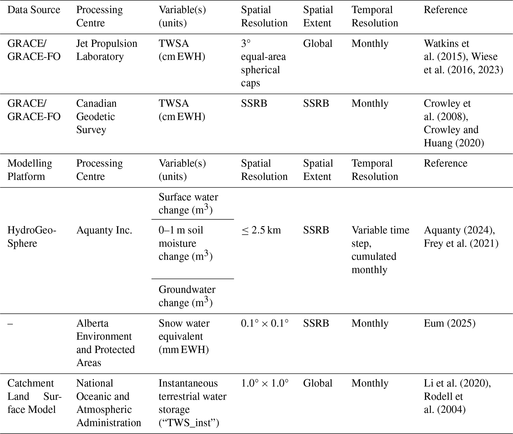
A summary of the variables, spatial and temporal resolution and extent, and appropriate references for the data and models used in the analysis is provided in Table 1.

Table 1 Summary of data and models used in the analysis.

A detailed description of each data and model source follows.

2.1 GRACE/GRACE-FO

The GRACE and GRACE-FO (henceforth “GRACE”) data used in the analysis are derived from the Jet Propulsion Laboratory Level-3 (JPL) monthly global mascon solutions (RL06.1M.MSCNv03) and extend from April 2002 to December 2019, which is the end of the HGS simulation interval. The JPL mascons are provided on a 0.5° × 0.5° grid but are derived from native 3° equal-area spherical caps placed on an elliptical Earth (Landerer et al., 2020; Watkins et al., 2015; Wiese et al., 2016, 2023). Included in the JPL mascon solution is a correction for glacial isostatic adjustment (GIA) based on the ICE-6G_D (VM5a) model from Peltier et al. (2018). The JPL mascon data represents TWSA in cm EWH with respect to a January 2004 to December 2009 baseline. This baseline period is referred to as the “GRACE baseline” and is used throughout the analysis to ensure consistent comparison of datasets. Gaps in the GRACE/GRACE-FO data record in between the two missions (11 consecutive months) and within the missions (22 months) have been filled using a machine learning technique described in Bringeland and Fotopoulos (2024) for continuous comparison. The JPL mascons (henceforth “JPL-M”) were spatially averaged to the study domain using a 0.5° × 0.5° gridded mask generated using basin boundaries based on Alberta Watersheds 2011 (Government of Alberta, Ministry of Environment and Sustainable Resource Development, 2011).

In addition to the JPL GRACE mascon solution, the GRACE solution produced by the Canadian Geodetic Survey (CGS) is also included. For brevity, this approach is referred to as the CGS method. This method incorporates the GRACE and GRACE-FO Level-2 spherical harmonic coefficient (SHC) solutions from the University of Texas Center for Space Research (CSR GRACE RL06 and GRACE-FO RL06.3) and applies a series of corrections and filtering steps (see below) to enhance signal quality while removing unwanted noise. Unlike mascon solutions, which impose predefined spatial constraints and model-based regularizations, the CGS approach provides greater processing flexibility while preserving the full range of geophysical and hydrological signals. One of its key advantages is the ability to define analysis regions based on hydrological boundaries, ensuring a more accurate representation of regional TWSA. In contrast, Level-3 solutions rely on a fixed grid-based structure (typically 0.25° to 0.5° spacing but with a true native resolution closer to 3°), which can lead to spatial leakage and inaccuracies near hydrologically complex regions. The CGS method overcomes this limitation by using spherical harmonic convolution and precise user-defined regions that can be aligned with watershed boundaries, though the inherent coarse resolution of GRACE prevents the complete elimination of signal leakage.

In the CGS method, missing degree-1 harmonics are replaced using externally derived estimates from GRACE Technical Note 13 (TN-13) (Sun et al., 2016; Swenson et al., 2008) while the C2,0 coefficient, which represents Earth's oblateness, is corrected using satellite laser ranging data (Loomis et al., 2019). To maintain consistency with other GRACE-derived estimates, GIA corrections are applied using the ICE-6G_D (VM5a) GIA model (Peltier et al., 2015, 2018). To further improve the accuracy of the SHC solutions, the destriping method of Crowley and Huang (2020) is applied to remove correlated errors, while a statistical filtering approach (Davis et al., 2008) eliminates high-degree spherical harmonic coefficients that lack statistically significant trends or seasonal signals. To suppress high-frequency noise for SHCs with statistically significant signals, a 167 km half-width (∼ 1.5°) Gaussian smoothing filter is applied (see Crowley et al., 2008). Spherical harmonic coefficients are converted from geoid height change to mass change following the Wahr et al. (1998) methodology. Finally, regional mass variations are extracted using spherical harmonic convolution, integrating mass change estimates over the defined study area (see Crowley et al., 2008). The final product is a monthly time series of TWSA, capturing both seasonal fluctuations and long-term trends in water storage.

As there is no “ground truth” data to determine the most accurate GRACE-derived product, multiple products are used to provide a range of estimates of GRACE-derived TWSA in the SSRB. This mitigates possible bias resulting from selecting one GRACE-derived product to compare to TWSA derived from the HGS model.

2.2 HydroGeoSphere (HGS)

The HGS model used in this study implicitly couples three governing equations, namely the three-dimensional Richards equation for variably saturated subsurface flow, the two-dimensional diffusion wave equation for overland flow, and the Manning's open channel flow equation for one-dimensional river flow, which are described more completely in Frey et al. (2021) and Aquanty (2024). Water exchange between the three domains occurs dynamically in response to hydraulic gradients that vary spatially and temporally across the domain. The HGS numerical solution utilizes a control volume finite element approach with adaptive time-stepping and OpenMP parallelization (Hwang et al., 2014).

The basis of the HGS model is an unstructured three-dimensional finite element mesh, which in the case of the SSRB model is composed of 11 subsurface layers and one surface layer with 2.5 km maximum node spacing away from river features, and 2 km maximum node spacing along river features. On each of the mesh sheets (surfaces) there are 51 279 nodes which form 101 214 finite elements per model layer. In total, over the 13 mesh sheets and 12 mesh layers, there are a respective 666 627 nodes and 1 214 568 elements. In the one-dimensional channel domain, there are 14 125 km of discretely resolved Strahler order 3 + rivers.

The three-dimensional structure of the model is presented in Fig. 2a. Topography is defined by a 15 m resolution LiDAR-based digital elevation model provided by Alberta Environment and Protected Areas (AEPA). Landcover distribution on the surface of the model is represented with 2015 North America Land Change Monitoring System 30 m resolution data (Latifovic et al., 2012). The top three subsurface layers are positioned at a 0.25, 0.5, and 1 m fixed depth from surface and represent spatially varying soil textures derived from Soil Landscapes of Canada (Soil Landscapes of Canada Working Group, 2010). Beneath the soil layers are two Quaternary geology layers based on material distribution defined by the Surficial Geology of Canada map-based dataset (Geological Survey of Canada, 2014) that extend down to bedrock. The lower six bedrock layers are derived from a simplified version of the 3D Provincial Geological Framework Model of Alberta, Version 2 (Alberta Geological Survey, 2019). Across the soil, Quaternary, and bedrock layers there are a total of 740 different porous media material zones configured into the model.

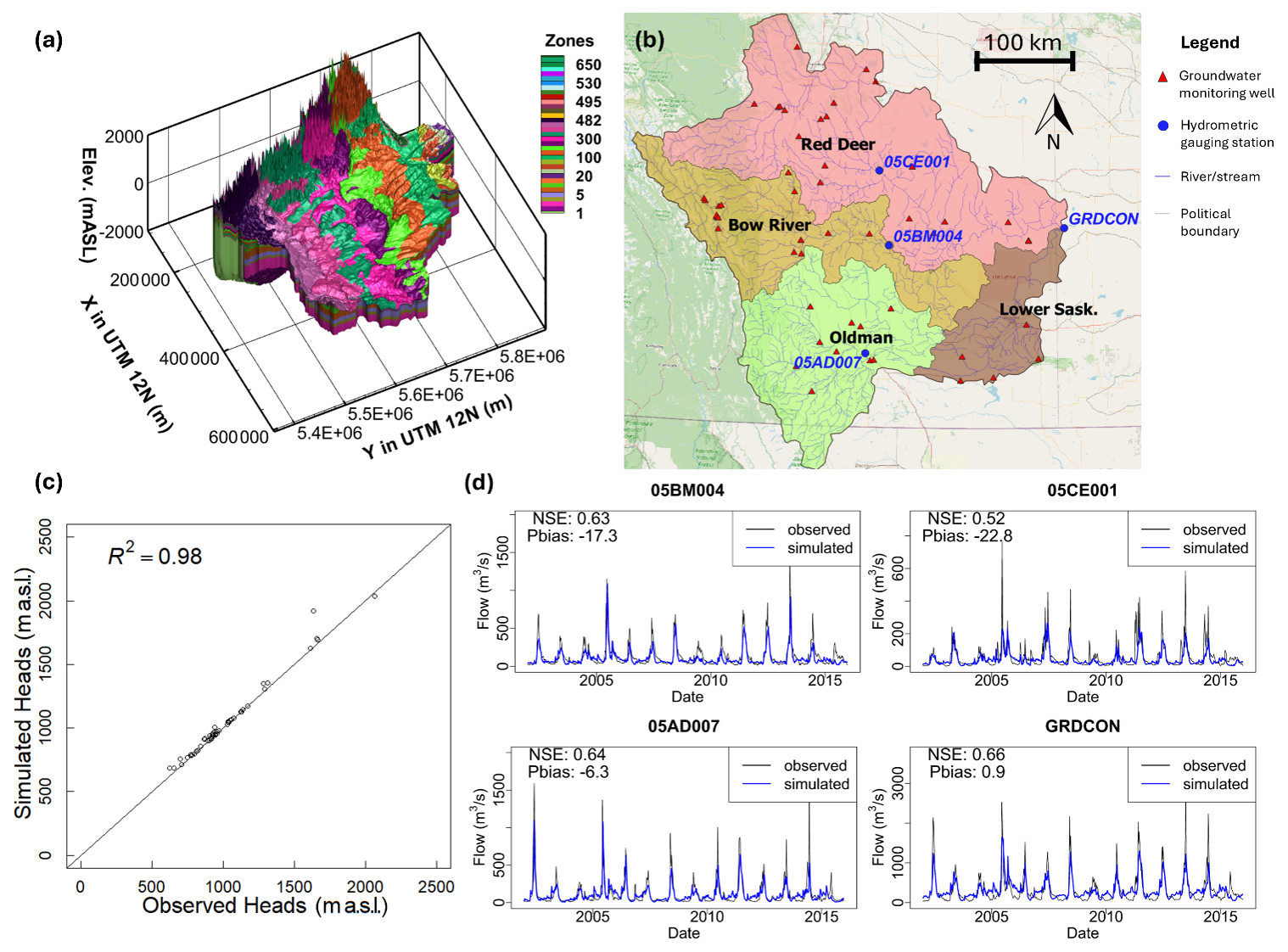
Figure 2 (a) Three-dimensional isometric perspective of the HydroGeoSphere SSRB model and its subsurface porous media zonation, (b) hydrometric gauging station locations in the Red Deer, Bow River, and Oldman River subbasins (circle markers), and at the SSRB outlet, and groundwater monitoring point (triangle markers) locations across the SSRB, (c) groundwater level simulation performance, and (d) surface water simulation performance at the four hydrometric station locations.

Forcing data for the HGS simulation, which includes liquid water flux (LWF) and potential evapotranspiration (PET), was derived from 0.1° (∼ 10 km) resolution daily transient Alberta hybrid climate data (Eum and Gupta, 2019). PET was calculated using a simplified Priestley-Taylor method that requires only precipitation and temperature (Alberta Agriculture and Rural Development, 2013). LWF was obtained from the sum of rainfall and snowmelt, with the latter calculated using a process-based snow model (Kienzle, 2008; Walter et al., 2005) modified by incorporating a S-curve approach (Kienzle, 2008) to consider diurnal temperature in a day, forced by the Alberta hybrid climate data.

For the purpose of this study, HGS model performance validation is based on 2002–2015 weekly transient naturalized river flow rates at four strategically positioned gauges that capture flow from each of the three major subbasins and at the SSRB outlet and average groundwater levels at 79 observation wells (Fig. 2b). Simulated groundwater levels show a strong correlation to measured levels (Fig. 2c), and simulated surface water flow rates align well with estimated naturalized flow data (Fig. 2d) based on both the Nash-Sutcliffe model efficiency coefficient (NSE) and percent bias (PBias) (Moriasi et al., 2007).

For comparison against GRACE TWSA data, HGS water storage changes in the surface domain, 0–1 m soil profile, and the groundwater system required averaging to monthly temporal increments and conversion to an anomaly value. The individual components of the HGS output were summed and then converted to EWH by dividing by the area of the SSRB. As the output from the HGS model represents the change from the previous timestep, the mean was removed and the cumulative sum of the changes was calculated in order for the resulting time series to represent water storage anomalies. Finally, the snow water equivalent (SWE) from Alberta Environment and Protected Areas was added, and the mean with respect to the GRACE baseline was removed, resulting in a HGS TWSA time series comparable to that of GRACE. The same process was applied to each of the storage components.

2.3 Catchment Land Surface Model

The output of the Catchment Land Surface Model (CLSM) from the NASA Global Land Data Assimilation System (GLDAS; Rodell et al., 2004) was used to provide an additional comparison for TWSA in the study area. GLDAS is an uncoupled land surface modelling system that incorporates satellite and terrestrially acquired data to produce a suite of hydrometeorological variables at a global scale. The CLSM V2.1 dataset used herein is provided on a 1.0° × 1.0° grid as a monthly averaged product (Li et al., 2020). The instantaneous terrestrial water storage (“TWS_inst”) variable was used in this analysis, spatially averaged within the study area and presented in cm EWH. The GRACE baseline was removed to ensure consistent comparison between datasets.

2.4 Oceanic Indices

Relationships between TWSA and several indices representing oceanic conditions were considered, namely the Oceanic Niño Index (ONI), the North Atlantic Oscillation (NAO), and the Pacific Decadal Oscillation (PDO). The ONI represents the 3 month average of the El Niño Southern Oscillation (ENSO) 3.4 index, which is the monthly sea surface temperature (SST) anomaly of the east-central tropical Pacific from 120 to 170° W. An ONI anomaly greater than + 0.5 °C represents El Niño conditions, while an ONI anomaly less than − 0.5 °C represents La Niña conditions (NOAA, 2019). The ONI is closely related to the PDO, an index which is computed using the extended reconstruction of SSTs produced by the National Oceanic and Atmospheric Administration (NOAA) and the Mantua PDO index (Huang et al., 2017; Mantua and Hare, 2002; Newman et al., 2016). The warm phases of the ONI and PDO are linked to warmer, drier conditions in the Canadian Prairies (McCabe and Dettinger, 2002; Shabbar et al., 2011). The NAO index represents the anomalies in the surface sea-level pressure difference between the Subtropical High and the Subpolar Low in the Atlantic Ocean (Hurrell and Deser, 2010). There does not appear to be a significant correlation between the NAO index and the hydrology of the Canadian Prairies (Chartrand and Pausata, 2020; Wittrock and Ripley, 1999), but this index is included in the analysis to ensure a comprehensive examination of possible drivers of hydrological trends in the SSRB.

3 Time Series Analysis Methods

Analysis of TWSA time series data includes some processing described herein. Signal decomposition (separation into annual, long-term, and residual trends) was done using least-squares to fit and remove a 31.7 nHz (1 year period) harmonic trend to the data, followed by a fit to remove the long-term linear trend. A continuous wavelet transform using the analytic Morse wavelet is used to assess the time-frequency content of the TWSA data (Lilly and Olhede, 2009, 2012). Lomb-Scargle power spectral density estimates are used to show dominant frequencies present in the data (Lomb, 1976; Scargle, 1982). As the continuous wavelet transform requires equally spaced data, the gaps in the CGS TWSA data were filled using a simple time series decomposition technique. The annual signal and linear trend (see Fig. 4) were calculated on a monthly interval. The gaps in the residual values were linearly interpolated at the same monthly interval. The sum of the annual, linear, and residual components resulted in the complete CGS TWSA time series. This data product was used for the continuous wavelet transform, as the Lomb-Scargle power spectral density estimates do not require evenly spaced data.

4 Results and Discussion

4.1 Terrestrial water storage anomalies

Figure 3 shows the HGS, GLDAS CLSM, and GRACE-derived (JPL and CGS) terrestrial water storage anomalies for the SSRB throughout the study period. The seasonal peaks in TWSA occur immediately prior to the spring thaw, in April/May, with the seasonal low coinciding with the end of summer, August/September.

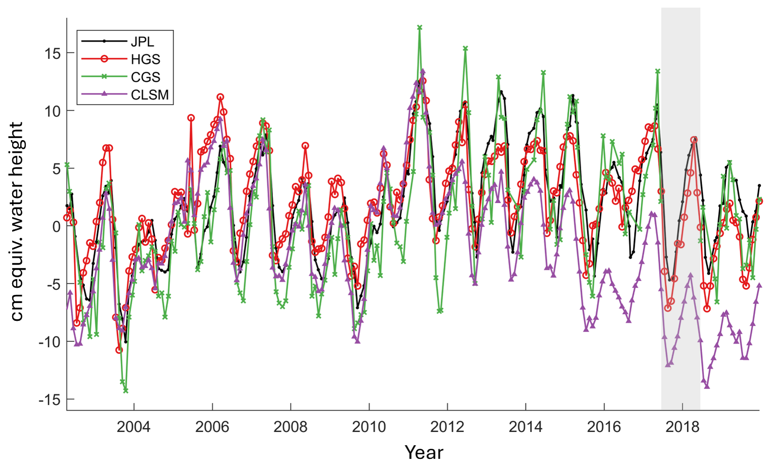
Figure 3 Terrestrial water storage anomalies in the SSRB derived from HydroGeosphere (HGS, red), JPL GRACE/GRACE-FO mascon solutions (JPL, black), CGS GRACE/GRACE-FO solutions (CGS, green), and the GLDAS CLSM product (CLSM, purple). Shading indicates gap between GRACE and GRACE-FO missions.

The HGS TWSA values approximately align with the GRACE-derived April/May peaks but overestimate late summer TWSA relative to GRACE. The CLSM TWSA increasingly underestimates TWSA relative to HGS, JPL, and CGS TWSA, especially after 2012. All four of the TWSA time series were decomposed into their annual, linear, and residual trends, which are shown in Fig. 4.

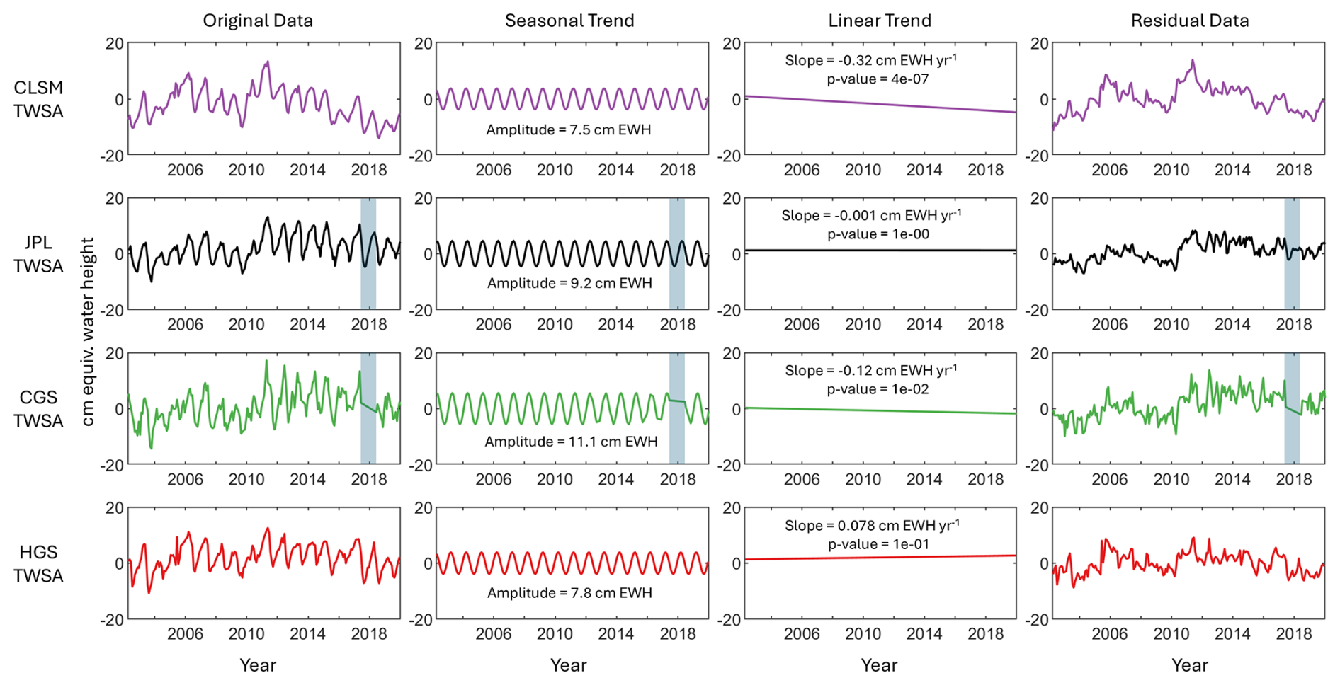
Figure 4 Signal decomposition of terrestrial water storage anomalies from the GLDAS CLSM product, JPL GRACE/GRACE-FO mascon solutions, CGS GRACE/GRACE-FO solutions, and the HydroGeoSphere model. Shading indicates gap between GRACE and GRACE-FO missions.

The GRACE-derived (JPL and CGS) time series have a larger seasonal amplitude (9.2 and 11.1 cm EWH, respectively) than the model-derived time series (HGS and CLSM, 7.8 and 7.5 cm EWH, respectively). The linear trend of the HGS time series is slightly positive, which differs from the slightly negative linear trends of the CGS and JPL TWSA time series. The method used to calculate the HGS TWSA values, which involves taking the cumulative sum of the anomalies in water storage, may contribute to this discrepancy, as the overestimation of any anomaly would be amplified throughout the study period. Results show that HGS TWSA estimates more positive late summer TWSA relative to JPL or CGS. The CGS TWSA has a slight statistically significant (p= 0.01) negative trend, though it is smaller in magnitude than the significant negative linear trend present in the CLSM TWSA. As HGS TWSA matches the GRACE-derived TWSA more closely than CLSM TWSA, the CLSM will be omitted from the rest of the analysis.

The interannual variations evident in the residual values in Fig. 4 (rightmost column) are similar throughout the different derivations of TWSA. The beginning (2002–2006) of the time series reflects the recovery from the 1999–2004 drought that affected the Canadian Prairie provinces (Bonsal and Regier, 2007) and is followed by a negative trend leading to the 2008–2010 drought (Sauchyn et al., 2020). Relatively wet conditions follow after 2010 until 2012, at which point a gradual decline in TWSA ultimately leads to drought in spring/summer 2019 (Sauchyn et al., 2020).

4.2 Time-variable frequency of water storage components

Constituent storage components of the HGS TWSA are shown in Fig. 5a, b, and c, while Fig. 5d shows the SWE storage in the SSRB with the GRACE baseline mean removed (i.e., shown as an anomaly).

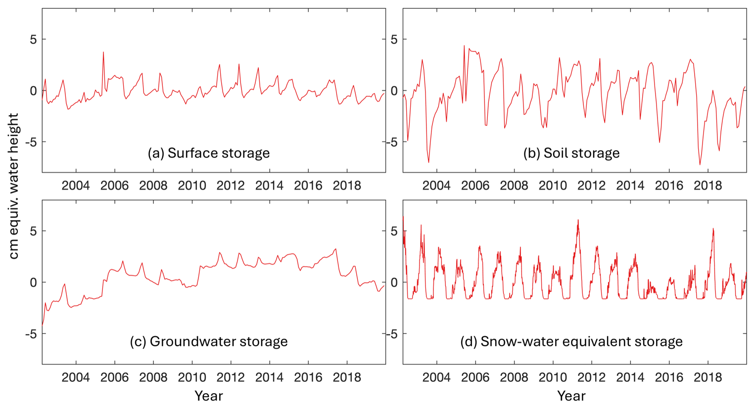
Figure 5 Cumulative HGS-based anomalies for (a) surface water storage, (b) soil moisture storage, and (c) groundwater storage, centred around the mean of the GRACE/GRACE-FO baseline period (January 2004–December 2009). (d) Snow-water equivalent storage is presented as an anomaly with respect to the same baseline but is not cumulated over the availability period.

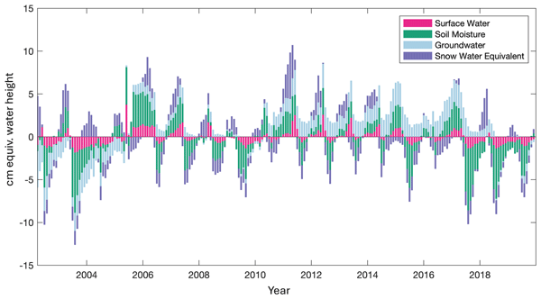
Soil storage in the SSRB shows the highest variability of any storage component, impacted both by seasonal variation and interannual trends. The SWE storage owes most of its variability to a seasonal fluctuation, but interannual differences in the amount of SWE storage are evident. The groundwater storage is the most “dampened” of any storage component, with a clear interannual trend and a low amplitude seasonal variation. Tangdamrongsub et al. (2021) had similar results (lower frequency, “dampened” trends in groundwater compared to soil moisture storage) when using a priori hydrological data to separate GRACE-derived TWSA into water storage components globally. The storage components are shown in a stacked bar chart in Fig. 6.

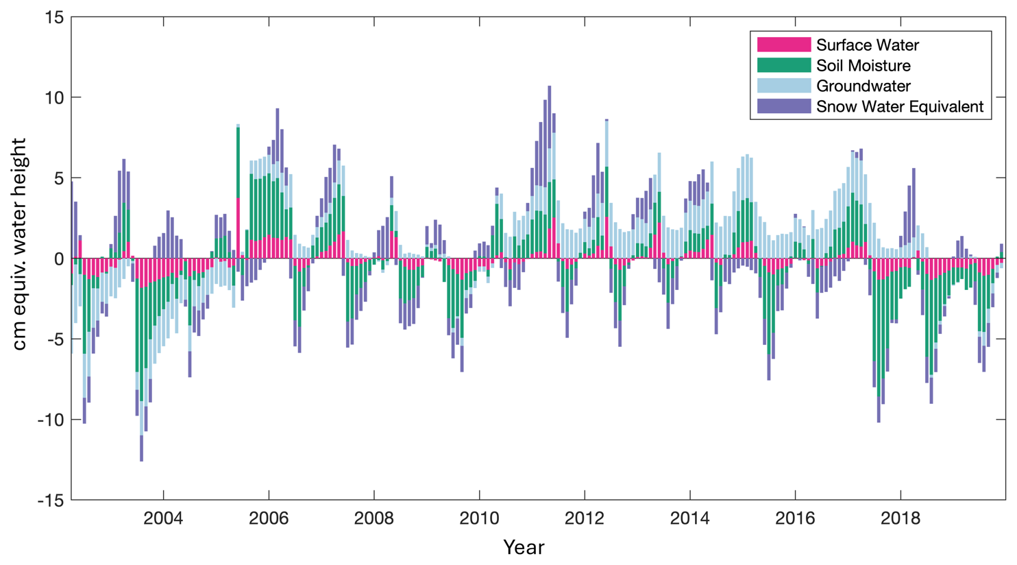
Figure 6 Stacked bar plot showing the monthly anomalies for different water storage components in the SSRB, including surface water (pink), soil moisture (green), groundwater (light blue), and snow-water equivalent (purple).

The separation of TWSA into its components allows for a higher resolution analysis of water storage dynamics than is possible with GRACE/GRACE-FO alone. This separation can allow for detailed analysis of agricultural or meteorological drought within different components of the water storage system and assessment of the contribution of pre-existing conditions to the vulnerability of an area to drought or flooding events. For example, the catastrophic flooding events of 2013 in southern Alberta may have been worsened by the positive groundwater anomalies (see Fig. 5) in the years leading up to the disaster, as excess runoff from heavy rainfall could not be offset by infiltration (Pomeroy et al., 2016). The largest proportion of the TWSA in the SSRB tends to be attributed to soil moisture storage, which is particularly apparent during times of drought (e.g., 2003, 2017, Fig. 5). Analysis of precursor conditions to extreme events can allow for better prediction and preparedness (Davitt et al., 2019). Climate change projections suggest that the Canadian Prairie region will be more prone to drought as temperatures rise, though increased precipitation is expected to increase groundwater recharge (Berg and Sheffield, 2018; Wheater and Gober, 2013; Zhang et al., 2020). The time-frequency content of the JPL TWSA, CGS TWSA, HGS TWSA, and HGS surface water, soil moisture, and groundwater are shown in Fig. 7. The power spectral density values in the Lomb-Scargle periodograms as well as the continuous wavelet transform amplitudes are normalized to the range of each individual parameter (Fig. 7). Note that edge effects impact confidence in the frequency content of the time series data near the start and end of the timespan, especially at longer periods.

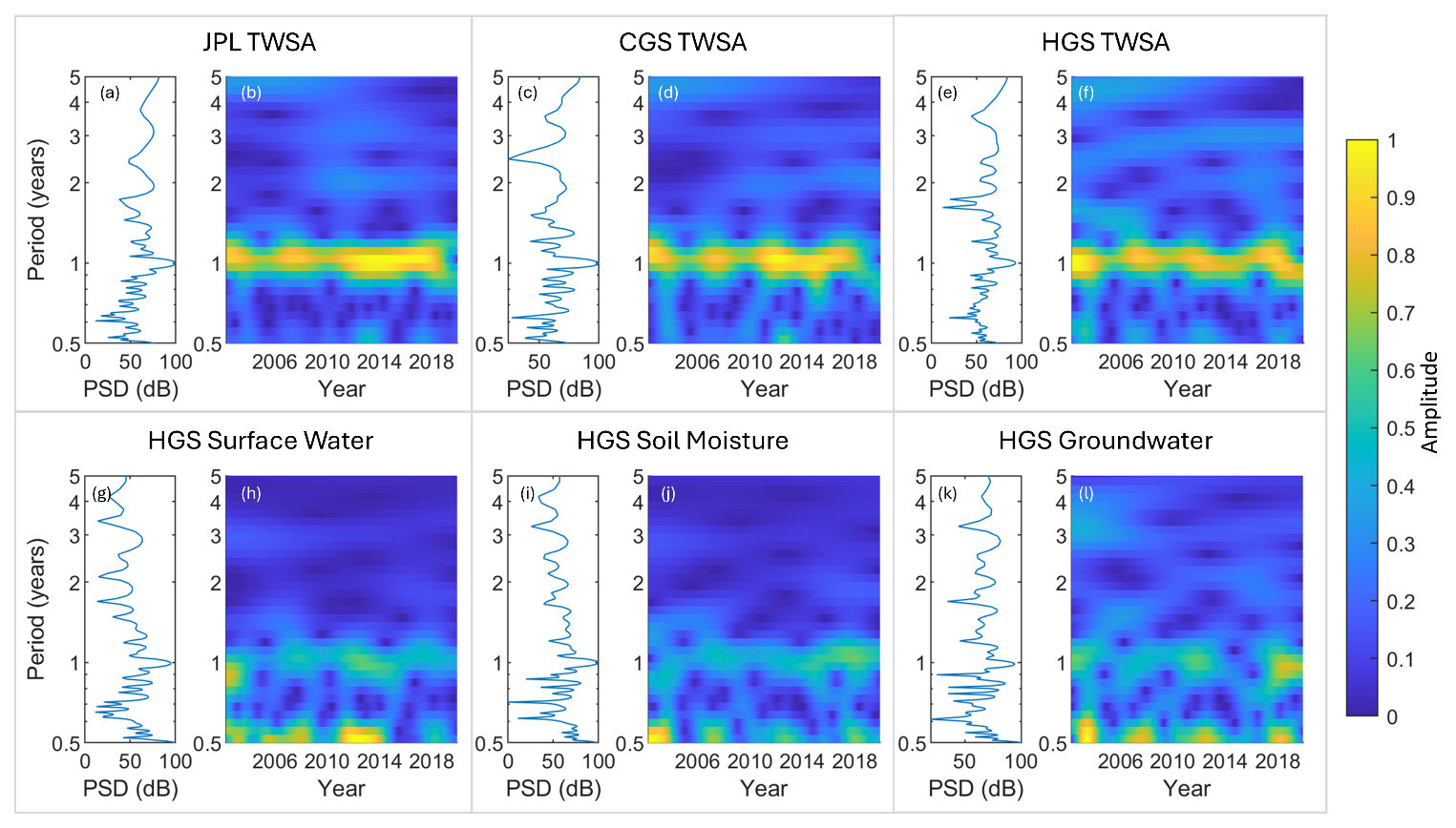
Figure 7 Lomb-Scargle periodograms (power spectral density (PSD), left) and continuous wavelet transforms (right) of the JPL TWSA (a, b), CGS TWSA (c, d), HydroGeoSphere TWSA (e, f), HydroGeoSphere surface water (g, h), HydroGeoSphere soil moisture (i, j), and HydroGeoSphere groundwater (k, l). Amplitude and PSD have been scaled from 0–1 and 0–100 dB, respectively.

The annual signal (period = 1 year) is the most prominent in all 6 parameters, though the period is inconsistent throughout the time series. The JPL, CGS, and HGS TWSA all reflect a peak in the amplitude of the annual signal around 2007, and again between 2010 and the end of 2017. The CGS and HGS TWSA show a fluctuation in the period of the annual signal between 2010 and 2017, where the annual signal is slightly longer than one year around 2012, slightly shorter than one year around 2014, and peaking at around 1.1 years between 2016 and 2017. The TWSA time series (Fig. 7a–f) contain interannual frequency trends with periods between 2–4 years, as is shown in the Lomb-Scargle periodograms (Fig. 7a, c, and e). The HGS storage components show similar power spectral density (PSD) peaks with periods between 2–3 years. The groundwater storage component shows a higher PSD in this range (Fig. 7k, 82 dB peak at period = 2.8 years) than the soil moisture and surface water components, which suggests that the interannual TWSA trends are more attributable to slow fluctuations in groundwater storage in the SSRB. None of the storage components have as strong an annual signal as the TWSA time series; the seasonal SWE trends likely contribute significantly to this frequency band.

4.3 Drivers of water storage change

To investigate relationships between prominent drivers of hydrological change and individual water storage components, the average annual anomaly for each driver (liquid water flux, evapotranspiration) and for each water storage component (surface water, soil moisture, groundwater, and SWE) was calculated to remove seasonal effects. LWF in this case refers to the sum of rainfall and snowmelt, and evapotranspiration represents the simulated actual evapotranspiration (AET); both parameters were generated as output variables by the HydroGeoSphere model. Plots showing the hydrological driver anomalies and water storage anomalies are presented in Fig. 8. Relationships between each pair of variables are modelled with a best fit line (red) and the upper and lower 95 % confidence bounds are shown (green).

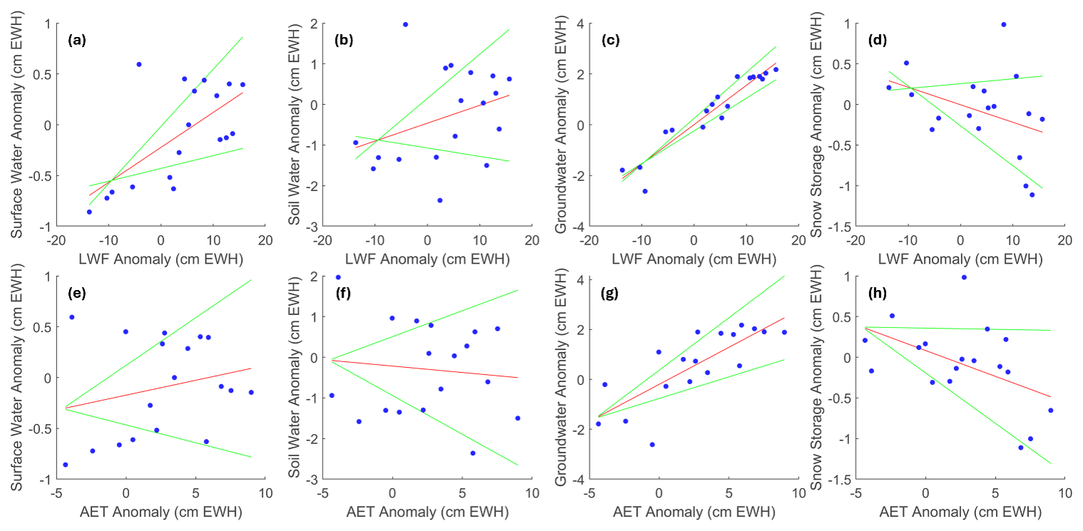
Figure 8 Annual anomaly (cm equivalent water height) in four components of water storage, namely surface water (a, e), soil storage (b, f), groundwater (c, g), and snow water equivalent (d, h), as a function of the annual anomaly in two drivers of hydrological change, liquid water flux (LWF) (a–d) and actual evapotranspiration (AET) (e–h). Linear trends (red) and the respective 95 % confidence intervals (green).

Some of the relationships between variables are straightforward and expected; anomalously high LWF leads to anomalously high surface water and groundwater (Fig. 8a, c). However, the relationships between AET and surface water and soil moisture are more complex. In this analysis, evapotranspiration is considered the “driving” variable, but positive anomalies in surface water and soil moisture imply more water is available to open air/vegetation, and thus, more water can be evaporated/transpired, leading to a positive AET anomaly. In this scenario, the surface and soil water components act as an independent variable driving AET. Conversely, AET anomalies can represent other meteorological anomalies such as temperature and latent heat flux, which should cause a negative anomaly in surface and soil water when increased. This complex relationship accounts for the wider confidence bounds shown in Fig. 8e and f. It is projected that evapotranspiration will increase in the Canadian Prairies as a result of a warming climate, which may affect the availability of surface water and soil moisture (Eum et al., 2017; Sauchyn et al., 2020). The increase in liquid precipitation associated with the projection of increased temperatures may offset this increase in evaporation and evapotranspiration, as is discussed by Roderick et al. (2015), referred to as the “aridity paradox”; the conflicting trends of increasing potential evapotranspiration and increasing precipitation with increasing temperature, and whether a warmer climate leads to more or less aridity. Spence et al. (2022) projects up to an 11 % decrease in maximum annual SWE per °C of warming in the grassland basins of the Canadian Prairies, which cover much of the SSRB within Alberta (He et al., 2023). Decreasing snowpack may reduce the amplitude of the annual signal in the TWSA (see Fig. 8), increasing the relative dominance of interannual trends in the SSRB. The trend of “wetter winters”, that is, a shortening snow season and lengthening rain season, is observed and projected in the Canadian Prairies as average temperatures increase due to climate change (Dumanski et al., 2015; Sauchyn et al., 2020).

Of all the oceanic indices considered in this study, the Oceanic Niño Index exhibits the strongest correlation with TWSA in the SSRB. To remove seasonal impacts and assess only the interannual trends, the HGS TWSA residuals (annual and linear trends removed) were smoothed using a 6 month moving average and were compared to the ONI. The results are shown in Fig. 9, along with the frequency content (Lomb-Scargle periodograms) of each of the ONI (right) and smoothed HGS residual TWSA (left). The ONI axis (right) has been reversed.

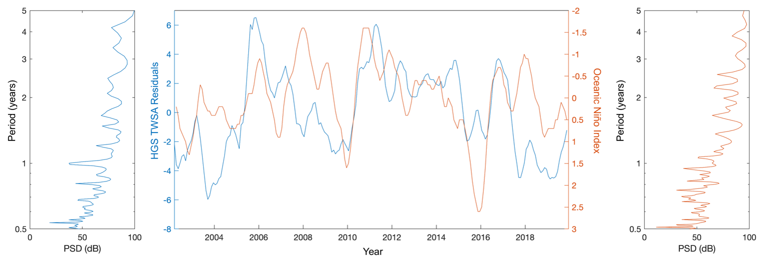
Figure 9 The Oceanic Niño Index (middle, orange) with the residual values (seasonal signal removed) of the HydroGeoSphere TWSA (middle, blue) in the study domain, smoothed using a 6 month moving mean. Note that the right y-axis in the centre plot is flipped. Lomb-Scargle periodograms of the smoothed HydroGeoSphere TWSA residuals (left, blue) and the ONI (right, orange).

The ONI has a moderate negative correlation (correlation coefficient $=-$ 0.38) with the smoothed HGS residual TWSA in the SSRB. This is consistent with McCabe and Dettinger (2002), Asong et al. (2018), and Shabbar et al. (2011) which suggest that a positive ONI anomaly is related to warm, dry conditions in the Canadian Prairies. The Lomb-Scargle periodograms of both parameters show a peak around the 2.7–3.0 year period (Fig. 7). This correlation explains some, but not all, of the interannual variability of TWSA in the SSRB. The El Niño Southern Oscillation has changed and is projected to continue to change temporally, with multi-year ENSO events becoming more frequent (Lu et al., 2025). Prolonged warm-phase ENSO events, linked with dry conditions in the SSRB, could increase the length and severity of drought. The characteristics of ENSO events are also projected to change in terms of location of the maximum sea surface temperature anomalies, with central Pacific El Niño events increasing with respect to eastern Pacific El Niño events (Yeh et al., 2009). It is unclear what effect this will have on the TWSA of the SSRB. The NAO showed no significant correlation with water storage components in the SSRB.

5 Limitations

While in-situ data was used to calibrate and validate the HydroGeoSphere model used in the study (see Fig. 2), the conclusions of this study rely mainly on model-based data and satellite observations. While many studies consider historical (Martz et al., 2007; Newton and Taube, 2023; Zare et al., 2022) or projected (Islam and Gan, 2014; Shrestha et al., 2021; Tanzeeba and Gan, 2012) hydrological trends in the SSRB, it is challenging to compare results directly, as the spatial and temporal extent of trend analysis differs. In addition, data from GRACE/GRACE-FO has no true “ground truth” comparison, so error can only be estimated theoretically. While the data from GRACE/GRACE-FO is processed to remove non-TWSA effects (e.g., glacial isostatic adjustment, atmospheric noise), any error in the models used to correct for these effects is propagated into the final estimate of TWSA. The results and conclusions of the study should therefore be interpreted within the context of the limitations described.

6 Conclusions and Future Outlook

Integrating both satellite gravimetry and high-resolution fully integrated GW-SW models allows for a comprehensive examination of water storage dynamics in the Canadian Prairies. Comparing GRACE- and model-derived TWSA reveals a possible 15 %–32 % underestimation of the seasonal amplitude in the HGS model and the GLDAS CLSM model, but the HGS model more closely matched the interannual trends present in the GRACE-derived TWSA. These interannual trends in the SSRB reflect large-scale events such as the 2008–2010 drought that was observed throughout the Canadian Prairies (Sauchyn et al., 2020). Separating TWSA into its constituent storage components using HGS allows for an examination of the influence of short- and long-term drought or flooding events on different water storage domains. This examination can provide insight into hydrological conditions that increase vulnerability to drought or flooding events, given anomalous meteorological events. Surface and groundwater are essential for agricultural and human activities in the SSRB and understanding the interannual and seasonal dynamics is imperative for sustainable water management, especially as climate change increases the likelihood and severity of extreme weather events. Understanding projected climate conditions and their relationships to components of water storage, such as snow water equivalent or groundwater, can help make sustainable water management strategies more robust.

Assessing the time-frequency content of components of water storage reveals an interannual harmonic trend with a 2 to 4 year period which is more prominent in the groundwater component of TWSA than surface water storage or soil moisture. This is likely related to global-scale oceanic and meteorological cyclicity which affects the average temperature and amount of precipitation, and thus groundwater recharge, present in the Canadian Prairies. The Oceanic Niño Index has a moderate negative correlation with the smoothed interannual trends present in the HGS-derived TWSA; both time series have a prominent 2.7–3.0 year period signal shown in the Lomb-Scargle periodograms. Interannual trends in TWSA in the SSRB may be impacted as the characteristics and timing of El Niño events change with a changing climate.

Accurate, high-resolution observations and models are crucial to understanding the impact of climate change on the quantity of surface and groundwater in the SSRB. Comparing satellite measurements to high-resolution hydrological models provides a method of independent calibration and validation. The HGS model differs from GRACE-derived TWSA in seasonal amplitude and long-term trends but reproduces the interannual trends observed by GRACE/GRACE-FO and can be used to examine different components of water storage and their relationships to oceanic and meteorological forcing conditions. As extreme meteorological events and long-term changes due to rising temperatures impact hydrology in Southern Alberta, a comprehensive characterization of water storage is imperative for sustainable water management for all anthropogenic and ecological activities (Wheater and Gober, 2013). Future work involves using the HydroGeoSphere platform to further assess TWSA in the different physiographic regions within the SSRB and to identify primary drivers of water storage change within these regions.