Setting the bar: benchmarks for model performances in large-sample hydrology

The availability of large-sample hydrometeorological datasets, now widespread across many regions worldwide, has changed hydrological catchment modelling. Assessing model performance is an essential component of any modelling exercise, and an important question is how to interpret performance measure values. Performances of uncalibrated bucket-type models vary significantly across regions and can reach NSE values of 0.8 or higher, particularly in humid or snow-dominated catchments. This implies that using a fixed value for a performance measure to judge model performance, as sometimes suggested in the literature, is inappropriate. Instead, one should consider that, given local hydroclimatic conditions and the quality of the available data, the performance we should expect from any model in a particular catchment can vary widely. At the same time, a perfect fit (NSE value of 1) is usually impossible to achieve due to errors and uncertainties in the model and data. Therefore, it is helpful to compare model performances to lower and upper benchmarks.

The purpose of this study was two-fold. First, we examined how to compute lower bounds, including determining appropriate ensemble sizes, assessing the effects of parameter ranges, deciding whether to use random or regional parameter sets, and evaluating how best to aggregate the ensemble of simulations. We also examined the relationships between lower and upper benchmarks and catchment characteristics. Secondly, we utilised these findings to compute both lower and upper benchmarks for many of the existing large sample datasets. By providing these values to the modelling community, we aim to facilitate the broader use of lower and upper benchmarks in large-sample hydrological modelling studies. We argue that these values are valuable as they provide a basis for evaluating model performance across the various large-sample datasets. This will allow assessment of model performance, considering what one could and should expect for a particular catchment.

1 Introduction

The availability of large-sample datasets has changed hydrological catchment modelling. Following the CAMELS dataset for the US (Addor et al., 2017; Newman et al., 2015), many similar datasets have been compiled for various countries (or regions) around the globe, such as Australia (Fowler et al., 2021), Chile (Alvarez-Garreton et al., 2018a), Brazil (Chagas et al., 2020) and Great Britain (Coxon et al., 2020a). These datasets are, for good reasons, widely used for developing new modelling methods (Kratzert et al., 2018; Lee and Kim, 2025), evaluating hydrological models (Pool et al., 2024; Rakovec et al., 2016), or model inter-comparison (Arsenault et al., 2023; Knoben et al., 2025). The assessment of model performance is an essential part of any of these applications and is usually done by comparison of observed and simulated streamflow time series. When assessing model performance, an important question is how to interpret the values of performance measures. Performance measures such as the Nash-Sutcliffe efficiency (NSE) (Nash and Sutcliffe, 1970), Kling-Gupta efficiency (KGE) (Gupta et al., 2009) or non-parametric efficiency (NPE) (Pool et al., 2018) range from minus infinity to 1. A perfect fit (value of 1) is usually impossible to achieve due to model and data errors and uncertainties. In the case of NSE, a value of zero can be considered a benchmark representing the prediction of a constant discharge equal to the annual mean discharge. Obviously, such a benchmark is not challenging and is easily outperformed in most catchments (Knoben, 2024; Melsen et al., 2025; Schaefli and Gupta, 2007). For example, we have previously shown that the performance of an uncalibrated bucket-type model varies significantly geographically, dropping below an NSE value of zero in only one out of ten catchments, and can reach NSE values of 0.8 or higher, especially in humid or snow-dominated catchments (Seibert et al., 2018). The latter observation implies that, besides the mean annual discharge being a benchmark that is easy to beat, using any fixed value for a performance measure to judge model performance (Crochemore et al., 2015; Moriasi et al., 2007; Palash et al., 2024) might not be appropriate, although it is still implemented in many modelling studies. Instead, one should consider that, given local hydroclimatic conditions and the quality of the available data, the performance we should expect from any model in a particular catchment can vary widely.

Therefore, it is helpful to compare model performances against lower and upper benchmarks (Seibert et al., 2018).While upper benchmarks suggest the performance that could be achieved for a certain period, given the input data and model structure, lower benchmarks indicate the performance that could be achieved without any local calibration or other use of the streamflow time series from the respective catchment. Local performance values can be scaled between these two benchmarks to assess how well a certain model simulation performs. Benchmarks can be based solely on data (e.g., statistical descriptors of the streamflow regime or rainfall-runoff ratios as applied in Knoben (2024) or on simulations from hydrological models. Here, we focused on model-based benchmarks because they allow us to generate both upper and lower benchmarks. To compute values for these benchmarks, one must first decide which model to use. While any hydrological model could be used, simple bucket-type models tend to be more suitable due to their relatively low data demand and ease of application to a large sample of catchments. Different models or an ensemble of models could be used. The use of a single model here is motivated by the observation that performance measures typically vary more between catchments than between models (Nicolle et al., 2014). In other words, as an indication of performances that could and should be achieved for a particular catchment, the choice of model is less crucial than the general decision to use lower and upper benchmarks and results are not largely affected by the choice of which model to use. Once the model has been chosen, computing the upper benchmark values is straightforward, as they are the values obtained by calibration to the individual catchments. Obtaining values for the lower benchmarks is a bit more challenging. One approach is to use ensembles of randomly chosen parameter sets. However, one must decide on parameter ranges and the ensemble size in this case. Furthermore, one must decide how to aggregate the performance of the ensemble, e.g., whether to use a median performance value of all ensemble members or the performance of the ensemble mean simulation as a lower benchmark.

The purpose of this study was two-fold. Firstly, we evaluated different approaches to derive lower benchmark values, and secondly, we provide upper and lower benchmark values for streamflow simulations based on existing large-sample datasets. We studied the question of appropriate ensemble sizes when computing model performances as lower benchmarks, the effect of varying parameter-value ranges, the difference between using random parameter sets and using regional parameter sets, and how to best aggregate the ensemble of simulations used for the lower benchmark. We also examined the relationships between lower and upper benchmarks and catchment characteristics. If such relationships could be established, they could be used to provide guidance on expected model performances in catchments for which the lower and upper benchmarks have not been previously computed.

Based on the above tests, we computed both lower and upper benchmarks for most of the currently existing CAMELS datasets (and intend to do so for new or updated datasets in the future). By providing these values to the modelling community, we aim to facilitate the broader use of lower and upper benchmarks in large sample hydrological modelling studies. We argue that these values are valuable as they provide a basis for judging model performance across the various CAMELS datasets. This would allow assessing model performances, considering what one could and should expect for a particular catchment. Such assessments are important, for instance, when one wants to judge the performance of a (more complex) model structure. While machine learning (ML) was not explicitly considered in this study, the benchmarks are suitable to evaluate ML approaches. ML could also provide alternative benchmarks to those based on bucket-type modelling presented in this study.

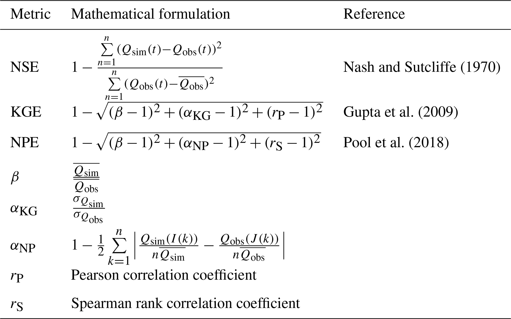
Table 1 Performance measures used in this study. Q_sim and Q_obs are simulated and observed discharge, t is the time step of the simulated and observed time series, I(k) and J(k) are the time steps when the kth largest flow occurs in the simulated and observed time series, n is the length of the simulated and observed time series, and σ is the standard deviation.

2 Data and Methods

2.1 HBV model

We used the HBV (Hydrologiska Byråns Vattenavdelning) model to obtain upper and lower benchmarks of model performance. The HBV model is a typical bucket-type model that has been widely used to simulate catchment runoff using time series of precipitation, temperature and potential evaporation (Lindström et al., 1997; Seibert and Bergström, 2022). The model consists of routines that represent hydrological processes related to snow accumulation and melt, soil moisture storage, groundwater and runoff generation, and routing along the stream network. Here, we used the software implementation HBV light, version 4, (Seibert and Vis, 2012) and a model variant with 13 free parameters.

In this study, the HBV model was applied in a semi-distributed manner to account for the elevation dependence of snow- and soil-water-related processes. Catchments were disaggregated into elevation bands of 200 m using data from digital elevation models (DEM).

The meteorological input data of precipitation and temperature were computed for each elevation band using fixed lapse rates of +10 % per 100 m for precipitation (Johansson, 2000) and −0.6° per 100 m for temperature (Wallace and Hobbs, 2006). Potential evapotranspiration was assumed not to vary with elevation.

2.2 Study catchments

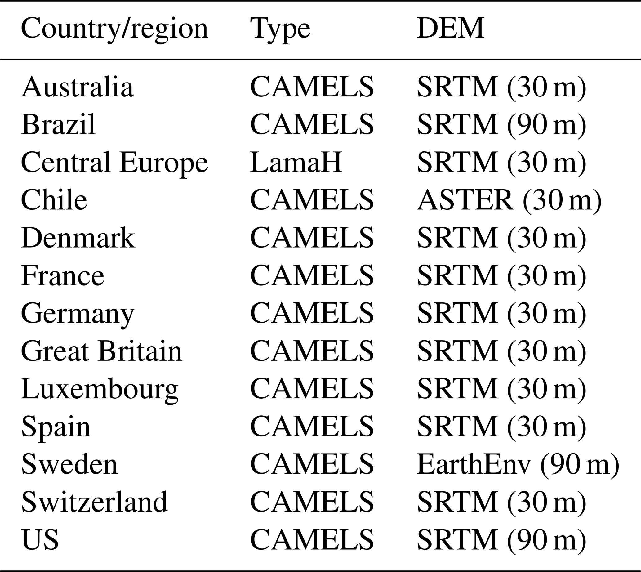
This study was based on thirteen large-sample datasets with daily hydro-meteorological time series and landscape attributes at the catchment scale. These included datasets for Australia (Fowler et al., 2021), Brazil (Chagas et al., 2020), Central Europe (Klingler et al., 2021b), Chile (Alvarez-Garreton et al., 2018a), Denmark (Liu et al., 2025), France (Delaigue et al., 2025), Germany (Loritz et al., 2024), Great Britain (Coxon et al., 2020a), Luxembourg (Nijzink et al., 2025), Spain (Casado-Rodríguez et al., 2026), Sweden (Teutschbein, 2024a), Switzerland (Höge et al., 2023), and the US (Addor et al., 2017; Newman et al., 2015) (Table 2). For model input, catchment-averaged time series of daily precipitation, temperature and potential evapotranspiration were used as provided by the different large-sample datasets. In some datasets, multiple time series of a variable are provided. In these cases, the variant used is explicitly stated in the Supplement (Table S4). For model evaluation, time series of observed catchment streamflow were available in the datasets.

Table 2 Datasets used in this study, the applied DEMs and the starting dates used for the simulations (note that the dates of the warming-up and simulation periods are provided in the data repository).

2.3 Benchmark simulations

The HBV model was used to simulate daily streamflow for each catchment using the continuous daily time series of precipitation, temperature, and potential evapotranspiration. The first one to two years were used as a warming-up period to obtain reasonable initial conditions for the storage components of HBV. The remaining years were then used for model calibration (upper benchmark) and evaluation (lower benchmark) with streamflow. Simulations were always run for the longest possible time for which concurrent data of precipitation, temperature and potential evapotranspiration were available. Thus, the calibration and evaluation period cover the same years. This approach follows the recommendation expressed by Shen et al. (2022): “Calibrating models to the full available data period and skipping temporal model validation entirely is the most robust choice and eliminates additional subjective decisions.” (p. 20). Note that the simulation periods differed across the datasets. As model performance values depend on the simulation period (Maier et al., 2023) the exact periods are provided in the data repository.

2.3.1 Lower benchmark

The lower benchmark performance for a catchment was based on simulations with randomly chosen parameter sets. We started by generating 100 000 random parameter sets, for which values were uniformly sampled within predefined parameter ranges corresponding to those used in previous studies (Seibert and Vis, 2012). The HBV model was run with each of these parameter sets and the catchment-specific model input data, resulting in 100 000 streamflow simulations per catchment. The simulations were evaluated by calculating three model performance measures, namely, the Nash-Sutcliffe efficiency, NSE (Nash and Sutcliffe, 1970), the Kling-Gupta efficiency, KGE (Gupta et al., 2009), and the non-parametric Kling-Gupta efficiency, NPE (Pool et al., 2018) (Table 1).

To analyse how many random parameterisations are needed for a representative lower benchmark, subsets of 1, 2, 5, 10, 20, 50, 100, 200, 500, 1000, 2000, and 10 000 simulations were randomly taken from the initial pool of 100 000 simulations. The selection of subsets was repeated 30 times. Model performance for each sample size (i.e., subset and sampling repetition) was aggregated in two ways: (i) by calculating the median performance of all simulations from a given sample size, and (ii) by calculating a single ensemble mean simulation from all simulations from a given sample size and subsequently calculating the performance of that ensemble mean simulation. This analysis of sample sizes could not be conducted for all catchments due to the high computational costs. Therefore, catchments were selected from the CAMELS-Australia, CAMELS-Brazil, CAMELS-Chile, and CAMELS-US datasets by randomly selecting a maximum of ten catchments from each Köppen-Geiger climate zone (first-order climate zones; Peel et al., 2007) represented in each CAMELS dataset. This resulted in 128 catchments in total (only eight catchments in the polar zone for CAMELS-US).

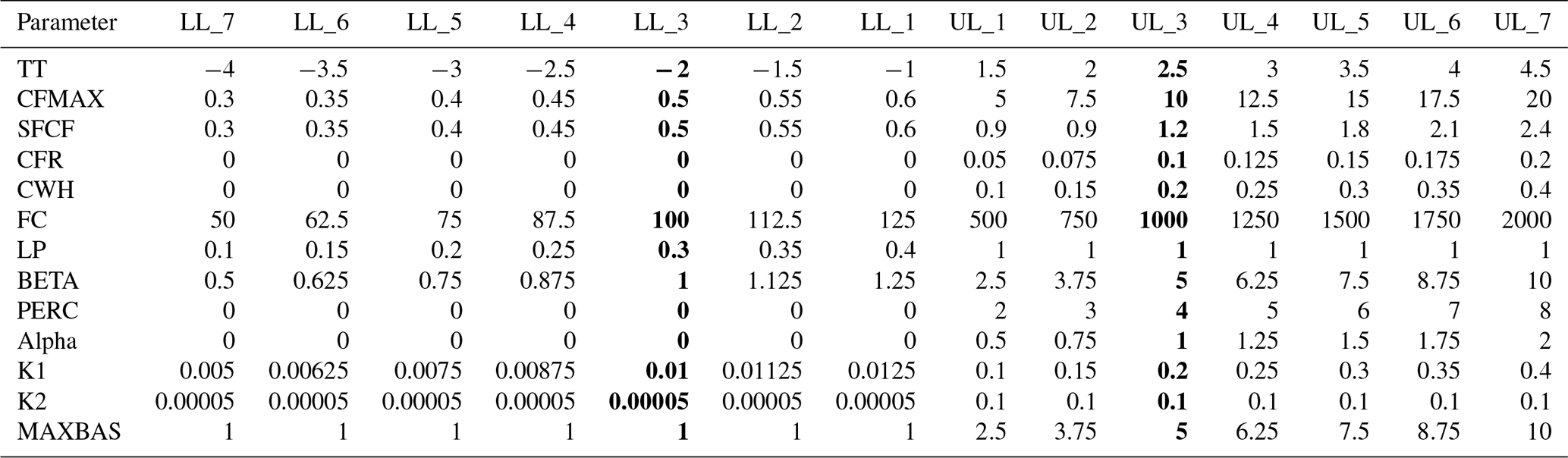
Furthermore, we tested the effect of the chosen parameter value ranges. For this, we tested four wider (i.e. range 4 to 7) and two narrower ranges (i.e. range 1 and 2) than the “standard” ranges (i.e. range 3) used in the rest of the study. The values for the lower and upper boundaries were varied linearly for each parameter in such a way that the parameter space for the widest ranges was about twice as large as the standard parameter space, and the parameter space for the smallest ranges was about half the size of the standard parameter space. The resulting ranges were slightly adjusted to cover the possible ranges (Table 3). For each range, ensembles of randomly selected parameter sets within that range were generated, and the performances were compared across the different ranges. This analysis was conducted for the same subset of 128 catchments as used for the sample size analysis.

Table 3 Limits of the seven parameter ranges used in the analyses. Lower (LL) and upper (UL) limits numbered from narrow distributions (Range 1) to wide distributions (Range 7). LL 3 and UL 3 (i.e. Range 3 in bold) correspond to the ranges used throughout this study.

Finally, we computed lower benchmark values based on regional parameter sets. The ensemble of these regional parameter sets contained the ten calibrated sets (see Sect. 2.3.2) of each other catchment within the respective CAMELS dataset. The performances of these ensembles were compared to those using the randomly chosen ensembles of parameter sets (using the standard parameter range).

2.3.2 Upper benchmark

The upper benchmark values were obtained by calibration for each individual catchment. The performance values thus provide an optimum of what is possible and must be expected to decrease over independent periods. The parameters were calibrated using the genetic algorithm implemented in the HBV model software (Seibert, 2000). The optimisation started with an initial, randomly generated set of 50 parameter sets (using the standard ranges, Table 3), which were recombined during 3500 model runs to maximise model performance. Separate calibrations were run using NSE, KGE, and NPE as performance measures. These model calibration trials were repeated ten times for each catchment and each performance measure, and the highest of the ten calibration performance values was used as the upper benchmark.

2.3.3 Spatial patterns of benchmarks

To explore regional differences in upper and lower benchmark values, we generated maps of model performance for each country and predicted model performance using random forest regression trees (Breiman, 2001). The random forest regression trees were run using the R-package randomForest (Liaw and Wiener, 2002), with 20 catchment characteristics (climatic, hydrological, and topographic) available in all CAMELS datasets as predictors for model performance. We conducted a ten-fold cross-validation in which 90 % of the catchments were used to train the random forest model and the remaining 10 % were used as independent test catchments. Each of the ten random forest models provided an estimate of variable importance based on the percent increase in mean squared error (% IncMSE) if that variable was randomly permuted for prediction. These values were averaged across all ten trees to quantify the importance of each variable for predicting upper and lower benchmark values. We share the ten fitted random forest trees (*.RData files) in the data repository (see data availability section), allowing readers to estimate the upper and lower benchmark values for any catchment of interest.

3 Results

3.1 Lower benchmarks: What is a suitable sample size?

The sample size considerably affected the lower benchmark performance values. As illustrated with an example catchment from the northeastern US, the median model performance of the ensemble at each sample size increased quickly when going from 1 to 10 or more ensemble members (Fig. 1a). When using only a few ensemble members, the variability of the performance among different realisations of the ensembles was high. The variability decreased with larger ensembles and stabilised at around 1000 parameter sets (Fig. 1b). This pattern was observed for both individual catchments (see Fig. 1a and b for an example) and for the aggregation of all catchments (Fig. 1c and d). Our finding means that using ensembles of 1000 or more parameter sets ensures that results for the lower benchmarks are stable and not notably affected by the randomness of generating the ensemble members. While we present the results only for NPE, the findings were consistent across all three performance measures tested here (results for all performance measures are provided in the data repository). In the remainder of this study, we thus always used 1000 ensemble members when computing lower benchmark values.

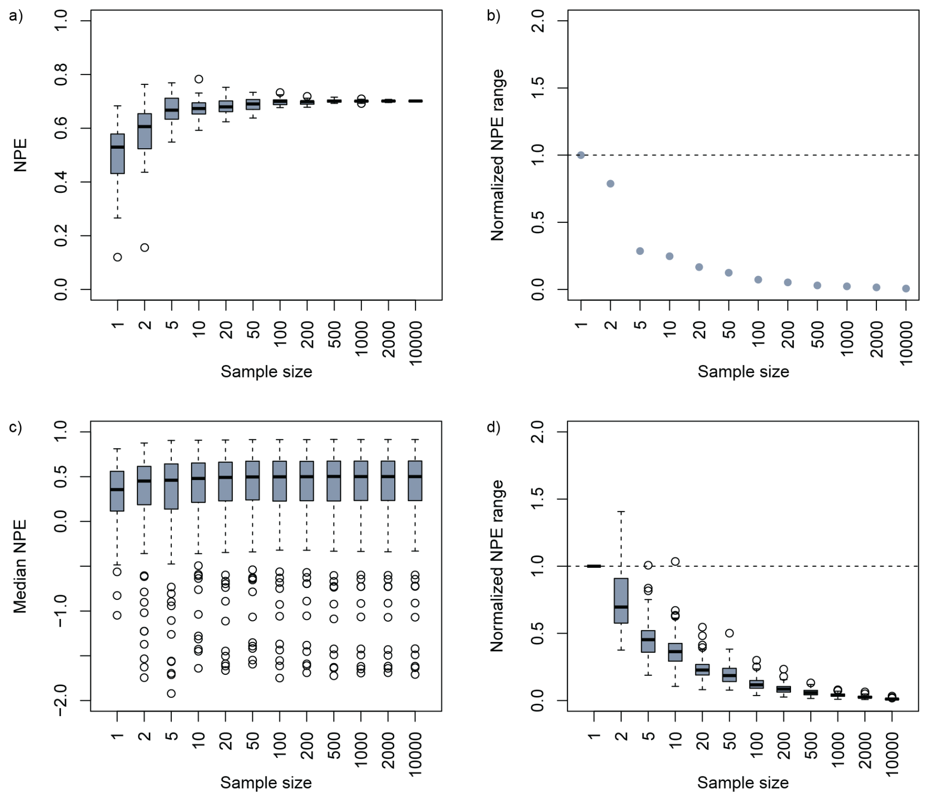
Figure 1 Impact of sample size on the lower-benchmark model performance NPE. Sample sizes range from 1 to 10 000 parameter sets, with values randomly chosen. For each sample size, the sampling was repeated 30 times. Results are shown for a catchment in the northeastern US in (a) and (b). (a) Box plots indicating the model performance values for each of the 30 sampling repetitions. (b) Range in model performances, calculated as the difference between the maximum and minimum value of the 30 sampling repetitions. For each sample size, the range was normalised by the range of sample size 1. Results are shown for all 128 test catchments from Australia, Brazil, Chile, and the US in (c) and (d), with (c) presenting median model performances NPE of the ten sampling repetitions for each test catchment, and (d) presenting the range in model performances.

3.2 Lower benchmark: ensemble mean versus median performance

The ensemble members at a chosen sample size need to be aggregated to obtain a single lower benchmark value. Using the median model performance of all ensemble members vs. the performance of the averaged time series of simulated runoff values makes an important difference (Fig. 2). For catchments with lower benchmark values for NPE below about zero, the median was, on average, better than the performance of the mean simulated time series. However, for NPE values above zero (i.e., reasonably well-performing catchments), the ensemble mean consistently outperformed the median of the individual simulations. A similar effect has been mentioned in previous studies with deep learning models (Heudorfer et al., 2025). Altogether, the ensemble mean performance exceeded the median performance in 94 %, 94 %, and 99 % of all catchments for NPE, KGE, and NSE, respectively.

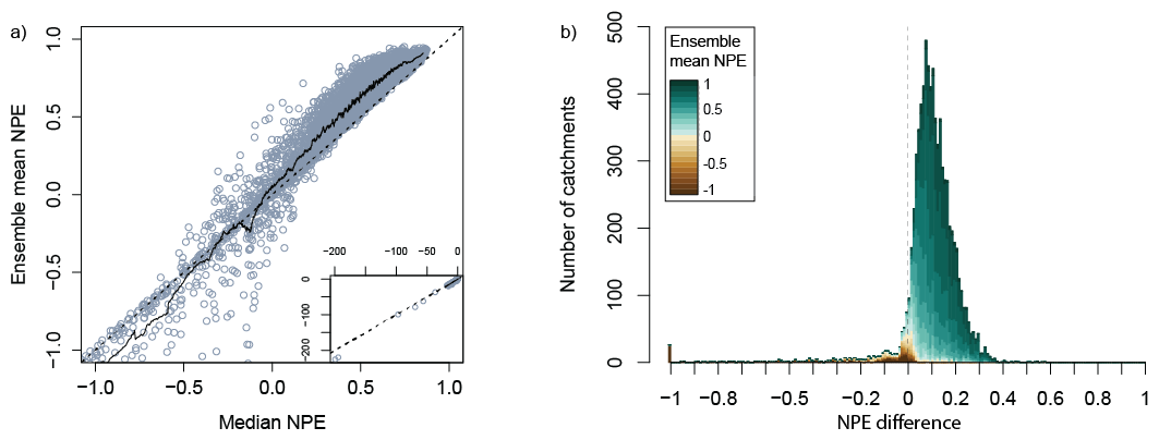
Figure 2 (a) Lower-benchmark model performance NPE when using the median NPE value of 1000 randomly chosen parameter sets vs. using the NPE value of the ensemble mean discharge simulation of 1000 randomly chosen parameter sets. The solid line represents the running mean value of the median, and the ensemble mean values (using a window of 51 catchments), and the dashed line indicates the 1:1 line. (b) Difference in NPE values when using the median NPE value vs. the ensemble mean value.

3.3 Effect of parameter ranges on lower benchmark values

Changing the parameter ranges affects the lower benchmark values when using random parameter values. Although the median model performance over all catchments did not vary much across the different parameter ranges tested (values between 0.42 and 0.52, with the maximum for Range 5), the mean model performance increased monotonically with increasing parameter range width (from −0.07 for Range 1 to 0.41 for Range 7). For individual catchments, there was considerable variation in the relationship between parameter-range width and the agreement between the ensemble mean of simulated streamflow and the observed time series (Fig. 3a). For some catchments, model performances increased for wider parameter ranges, whereas for other catchments, a decrease in performance towards the wider parameter ranges could be observed. Therefore, instead of examining mean model performances, we compared the mean absolute difference across performances when using different ranges for the individual catchments. The results of this analysis indicated that when changing ranges drastically, performance values may vary considerably. However, as long as these differences in the ranges were not too large, the performance values generally agreed (Fig. 3b).

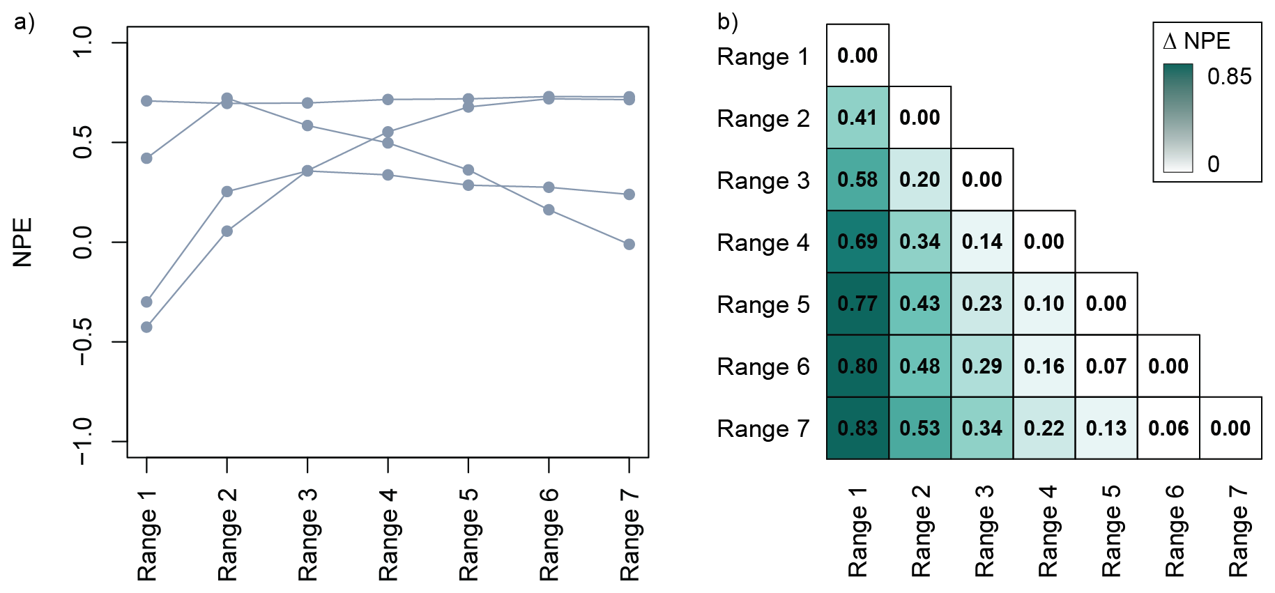
Figure 3 Effect of parameter ranges on the performance (NPE) of the lower benchmark. (a) NPE-values for four example catchments, and (b) pairwise mean absolute differences of the NPE values (based on all 128 test catchments from Australia, Brazil, Chile, and the US). Note that Range 1 corresponds to the parameter ranges between LL_1 and UL_1 Range 2 corresponds to the parameter ranges between LL_2 and UL_2, etcetera (see Table 3 for definitions and values). In other words, ranges varied from narrow (Range 1) to wide (Range 7).

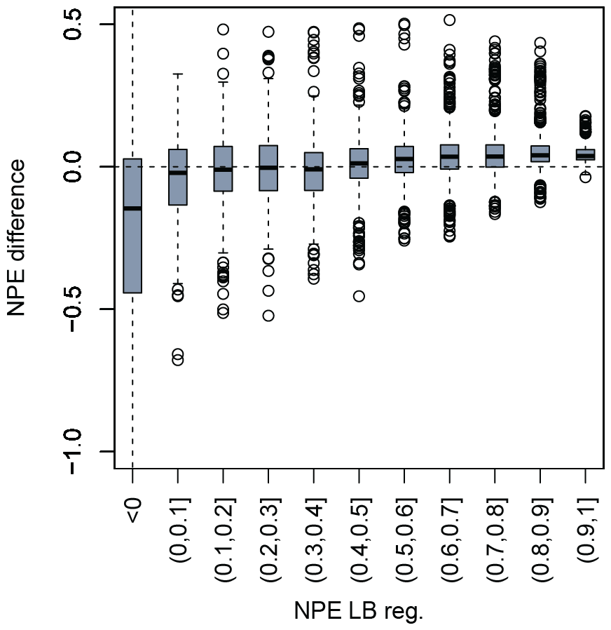
Figure 4 Differences of the lower benchmark values (NPE) when using regional vs. random parameter sets, plotted as box plots for classes of catchments with different NPE values for the regional parameter sets.

3.4 Lower benchmark values from regional parameter sets

The performances obtained with the so-called regional parameter set ensembles correlated well with those from random parameter sets. For catchments for which the random parameter set ensembles resulted in NPE values above 0.5, the regional parameter set ensembles resulted, on average, in higher NPE values with differences of about 0.05 NPE units. However, for catchments where the random parameter ensembles resulted in lower NPE values, using regional ensembles did not improve model fits or resulted in even lower NPE values (Fig. 4).

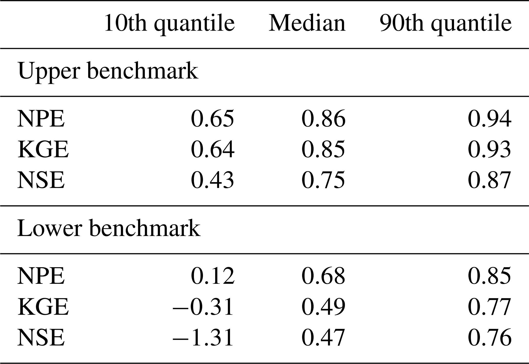
Table 4 Summary of model performances (NPE, KGE, and NSE) for the upper benchmark and lower benchmark (represented by the ensemble mean of 1000 parameterizations). Values are based on all CAMELS datasets used in this study.

3.5 Upper and lower benchmark values

The upper and lower benchmark values varied widely across the catchments in the different CAMELS datasets (Fig. 5 and Table 4). Looking at all CAMELS datasets, on average (median), the upper benchmark values for NPE were 0.86 (KGE 0.85, NSE 0.75) and for 90 % of all catchments, the upper benchmark values were larger than 0.65. The lower benchmark values were, as expected, clearly lower. Here, the median NPE was 0.68; for 90 % of the catchments, the NPE was greater than 0.12, and for 10 % of the catchments, values were greater than 0.85. There was considerable variation across the different CAMELS datasets, especially for the lower benchmarks (Fig. 5b).

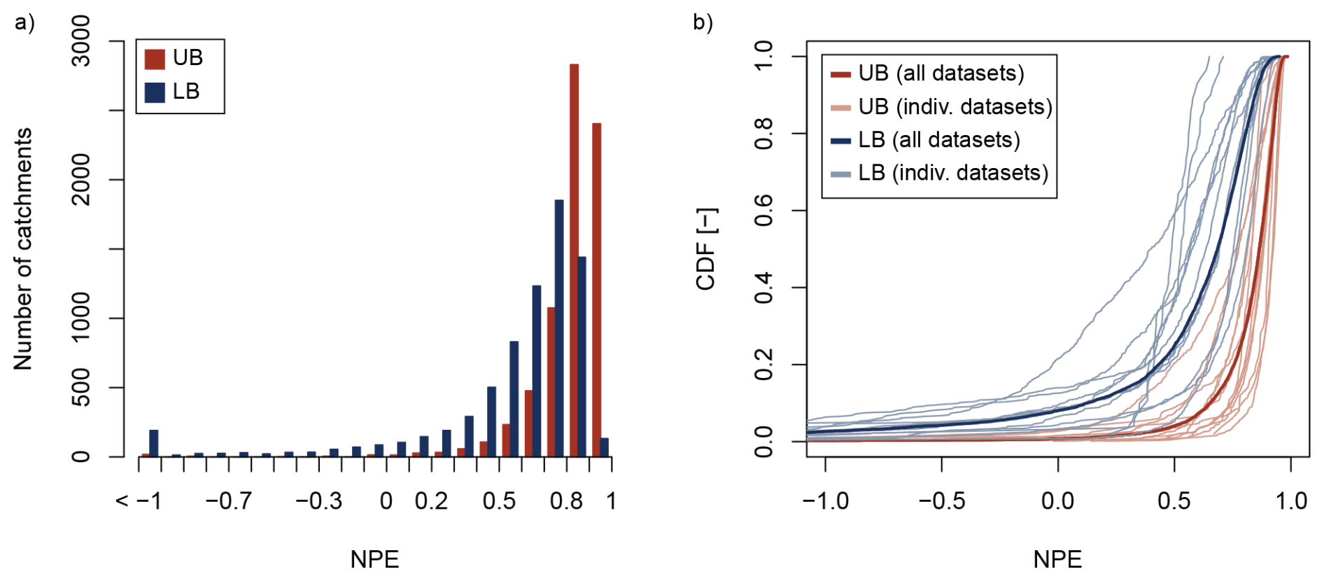
Figure 5 Model performances (NPE) for the upper benchmark (UB) and lower benchmark (LB; represented by the ensemble mean of 1000 parameterizations). (a) Histogram showing the values for all CAMELS datasets. (b) Cumulative distribution functions (CDFs) for all CAMELS datasets and the individual CAMELS datasets.

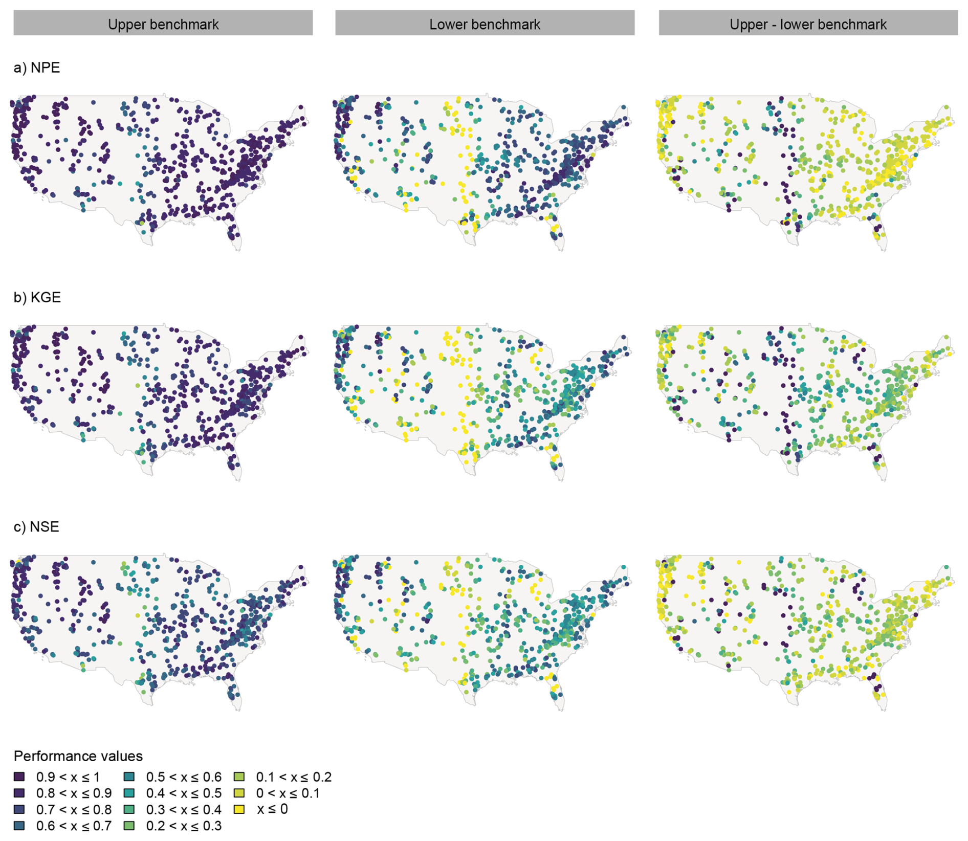
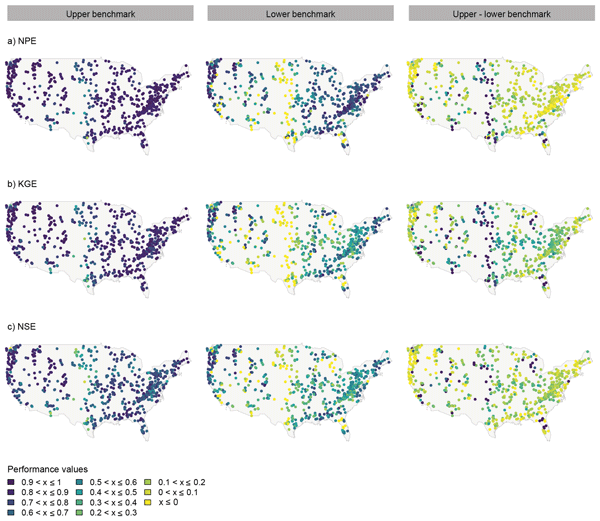
Figure 6 Spatial patterns of model performance for catchments in the contiguous United States (CAMELS-US dataset) for the upper benchmark (first column), lower benchmark (represented by the ensemble mean of 1000 parameterisations, second column), and the difference between upper and lower benchmark (third column). Values are shown for (a) NPE, (b) KGE, and (c) NSE. Spatial patterns for the other CAMELS datasets used in this study are provided in the Supplement (Figs. S1–S12).

Within the different CAMELS datasets, the lower benchmark values varied more than the upper benchmark values. For the CAMELS-US dataset (Fig. 6), for instance, the lower benchmark was higher in regions along the east and west coasts, where it approached the upper benchmark. In contrast, much lower values were obtained for the lower benchmark in the central parts of the country. The larger variability of the lower benchmark than the upper benchmark, also observed for the other datasets (see Figs. S1–S12), implied that the pattern of differences between the upper and lower benchmarks largely followed that of the lower benchmarks (Fig. 6).

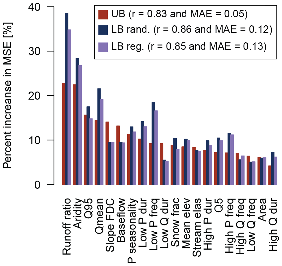
Figure 7 Importance of catchment attributes for predicting model performance NPE for the upper benchmark (UB), the lower benchmark represented by the ensemble mean of 1000 parameterizations (LB rand.), and the lower benchmark based on regionally donated parameter sets (LB reg.) of all CAMELS datasets using a random forest model. The importance of each variable is expressed in terms of the percentage increase in mean squared error (MSE) if that variable is randomly permuted for the prediction of NPE. If a catchment attribute is more important, the related percentage increase in MSE is higher. The performance of the random forest model for the test data was quantified by the Pearson correlation coefficient (r) and the mean absolute error (MAE).

3.6 Predictability of upper and lower benchmark values

The upper and lower benchmark values (derived using randomly selected values within the standard parameter ranges) were related to catchment characteristics. The random forest analysis, which was based on all catchments and datasets, indicated that the most important variables for predicting upper benchmark performance were runoff ratio, aridity, high flows (quantified by Q₉₅) and mean flow (Q_mean) (Fig. 7). Similarly, the most important variables for predicting the lower benchmark performance were runoff ratio, aridity, mean flow (Q_mean), and low precipitation frequency. In general, there were tendencies for model performances to increase with increasing runoff ratios, mean flows, and Q₉₅, but to decrease for increasing aridity, suggesting that catchment wetness exerts a major control on both lower and upper benchmark values (Fig. 8). However, there was a huge variability, and the individual correlations were rather weak, highlighting the importance of simultaneously considering a range of variables for predicting model performance. More details on the performance of the random forest models for all three objective functions are available in Fig. S13 and Tables S1–S3.

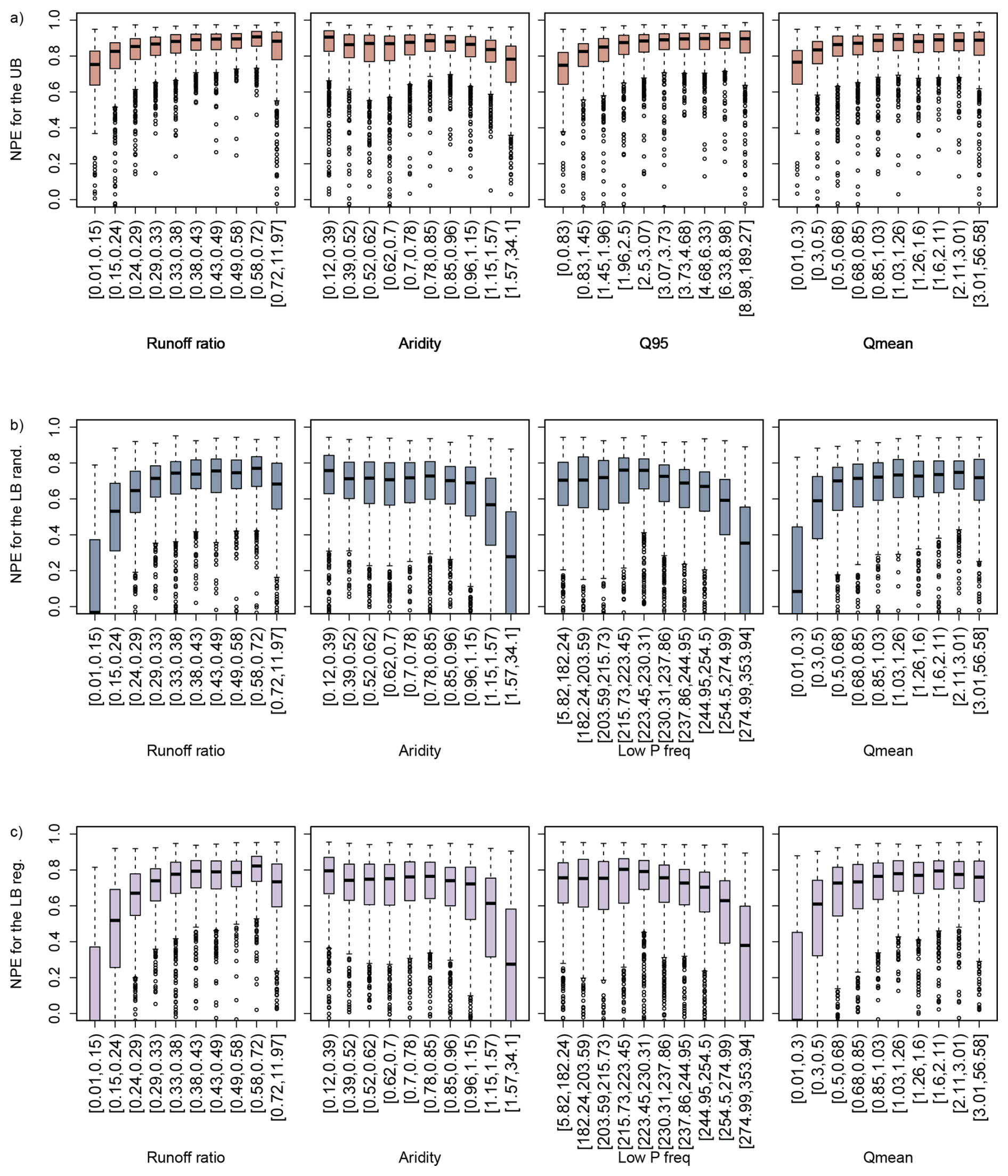
Figure 8 Relationship between model performance NPE and the four most important variables for predicting NPE of all CAMELS datasets with a random forest model. Relationships are shown for (a) the upper benchmark (UB), and (b) the lower benchmark represented by the ensemble mean of 1000 parameterizations, and (c) the lower benchmark based on regionally donated parameter sets.

4 Discussion

4.1 Why use benchmarks?

Often, it is suggested to rate model performance based on fixed values of an objective function (e.g., NSE) that do not vary among catchments (Moriasi et al., 2007). This highly cited paper reflects the widespread habit in the hydrological modelling community of judging model performances based on the absolute values of performance measures without comparison with local conditions. The use of such absolute values is appropriate in some cases, e.g., when the aim is to get an indication whether the model is fit for its intended purpose (such as flood peak simulations for flood management). However, we argue that we need to examine model performance in more detail, especially when comparing model performance across different catchments. Here, we need to consider that the model performance achievable for a particular catchment varies widely across catchments (Fig. 4).

Various reasons can lead to such variability. For example, as shown in our random forest analysis with over 6000 catchments from 13 countries worldwide (Figs. 7 and 8), a modeller should generally expect higher model performance values for relatively humid catchments than for water-limited catchments. This is because in humid catchments the discharge, both observed and simulated, is much more constrained by the precipitation than in arid catchments, where evaporation can play a much more important role in relative terms. Although this is a well-known phenomenon (e.g., Poncelet et al., 2017), it is rarely considered or explicitly mentioned when assessing the goodness of fit of a model.

Furthermore, expectations should vary with the quality or resolution of the model's input and output data. For example, discharge simulations tend to improve with increasing resolution of the meteorological input or increasing spatial density of gauging stations used for model calibration (Girons Lopez and Seibert, 2016). Also, periods of disinformative observed discharge data can considerably challenge model calibration (Beven and Westerberg, 2011). Therefore, it is essential to overcome the common practice of interpreting model performance metrics, such as NSE or KGE, without benchmarking.

4.2 Guidance for computing benchmarks with bucket-type models

One argument against using benchmarks is the additional effort. Our study addresses this issue in two ways: (1) we provide computed values for several CAMELS datasets and, thus, for a large set of catchments, (2) we provide the trained random forests so that benchmarks can be estimated for catchments not included in the dataset. Furthermore, we provide guidance on computing benchmark values, especially on how many ensemble members are needed to obtain lower benchmark values. The findings of this study allow limiting the number of ensemble members for computing lower benchmark values. Based on our results and to ensure robust results, we recommend using 1000 random parameter sets for the ensemble used to compute the lower benchmark values. While more runs would be possible, such guidance helps limit the number of model runs required.

Each ensemble member results in a simulated runoff time series, and for aggregation, one can use the mean or the median. While the latter might be less affected by outliers, the mean has the crucial advantage of preserving the water balance. We therefore used the mean to aggregate the ensemble simulations into a single simulated runoff time series. Based on comparisons between the median performance of individual model runs and the performance of the ensemble mean, we found that the latter produced better results in catchments, where simulated runoff agreed reasonably well. While the ensemble mean generally is the stronger benchmark than the median, it has the disadvantage that it is not directly related to any physically realizable parameter set.

Our results demonstrated that performance values for the lower benchmark varied as the parameter ranges were modified. This could be interpreted as an argument for using regional parameter sets to compute lower benchmark values. In this case, an ensemble of parameter sets calibrated for other catchments in the same region (or country) is used to produce an ensemble-mean time series (Seibert et al., 2018). Since optimised parameter sets are used in this case, the initial parameter ranges are less influential. However, using ensembles of randomly generated parameter sets has the important advantage that no other catchments are required to compute the lower benchmark values.

We argue that both upper and lower benchmarks should be used. The former is important as, in reality, a value of 1 is usually not possible even for a “perfect” model. Comparing performances against a lower benchmark is even more important, as the performance that will be obtained with a completely uninformed model varies largely depending on local hydroclimatic conditions.

When comparing performances of some other model with the upper benchmark, it is fully possible that performance values are better than those obtained as the upper benchmark, i.e., here the performance of the calibrated HBV model. While this might be a result of larger complexity and, thus, flexibility (e.g., more free parameters, including the risk for overparameterization), this situation can also indicate that the tested model is a more suitable representation of the hydrology of this catchment. ML approaches may offer further opportunities to improve runoff simulations.

For some catchments, upper and lower benchmarks might also be very close. In this case, using relative model performances (i.e., scaled between UB and LB) might result in unrealistically large values. In such cases, it is important to distinguish between the situation where both UB and LB are very low, indicating that either the HBV model is unsuitable for a catchment or that there are severe data quality issues, and the situation where both UB and LB are relatively high, indicating that any model could provide a good simulation of observed catchment streamflow.

Table 5 Links to the datasets used in this study.

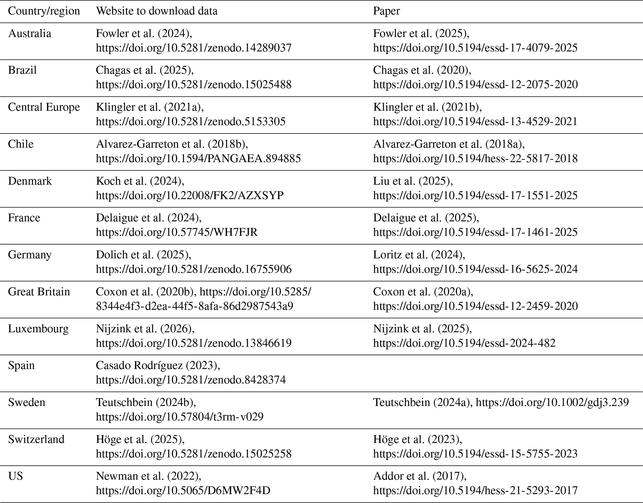
All links last accessed on 10 September 2026.

4.3 Limitations of our study

The benchmark values presented in this study are dependent on the model and settings used. The upper benchmarks are not the absolute best model performances and can be exceeded by other models, especially if these have more degrees of freedom (calibration parameters). However, the values still provide useful guidance, as different models and settings will not dramatically alter them. For the CAMELS-US dataset, for instance, very different model setups tend to yield similar performance patterns (Knoben et al., 2025). Comparing three bucket-type models for catchments in Tunisia, Dakhlaoui et al. (2017) found relatively small differences in model performance between the models. The same applies to studies with different GR4J versions in France (de Lavenne et al., 2016) or different models in Australia (Fowler et al., 2020).

Admittedly, the benchmarks as discussed here evaluate model performance only with regard to runoff. There might be other (internal) variables which could also be used to evaluate model performance (i.e., internal model consistency). This could be done in a similar way as proposed here with upper and lower benchmarks. However, for hydrological catchment models, it is common to focus on runoff.

5 Conclusions

Based on our study, in which we computed lower and upper benchmarks for 13 large-sample datasets around the globe, we recommend that using lower and upper benchmarks should become part of good modelling practice. The performance of lower benchmarks (i.e., uninformed models) can vary largely and in some regions, these lower benchmarks can reach surprisingly high values, meaning that the same fixed value of performance measures is not applicable to judge model performance in every catchment. Upper benchmarks should be used as perfect fits are not possible in practice.

We provide lower and upper benchmarks for several large-sample datasets together with this publication. However, one might want to compute benchmarks for other catchments or time periods. When computing lower benchmarks, we found that a limited number of ensemble members is sufficient; we recommend using 1000 members. The lower benchmark values varied as the parameter ranges were changed; therefore, it is essential to specify these ranges when computing them. However, values generally agreed when the ranges were not changed dramatically. Still, the effects of parameter ranges might be an argument for using ensembles of calibrated regional parameter sets. These ensembles also provide a more challenging benchmark than randomly generated parameter sets. Finally, we recommend aggregating the ensemble members by calculating the ensemble mean time series and using the corresponding performance metric, rather than the median performance of the ensemble members as a lower benchmark.

While the exact values of the lower and upper benchmarks will vary somewhat, we argue that this should not be used as an argument against using such benchmarks altogether. Here, we provide both benchmark values and guidelines for computing them. In other words, this study provides helpful guidance on calculating upper and lower benchmarks with any model for any catchment.