Integrating propagation and recovery dynamics into groundwater drought vulnerability assessment through exposure, pressure, and aquifer system response

Groundwater drought reflects the combined influence of meteorological forcing, aquifer memory, hydraulic connectivity, and anthropogenic modification. This study develops a hydrogeologically informed statistical framework that integrates temporal groundwater-drought characteristics with spatial indicators of Exposure, Pressure, and environmental Sensitivity. Standardized Precipitation and Groundwater Level Indices were analysed at 3-, 6-, and 12-month aggregation scales for 16 piezometers grouped into shallow unconfined, intermediate confined, and deep confined aquifer systems. The shallow unconfined aquifer showed the strongest SPI–SGI association, whereas the deep confined aquifer exhibited weaker correlations, longer drought persistence, and no observed recovery within the available record. These contrasts are consistent with differences in aquifer memory and hydraulic conditions, but conclusions concerning the deep system remain exploratory because it is represented by only two monitoring wells and may also be affected by sustained anthropogenic pressure. The Drought Impact Potential Index (DIPI) combines piezometer-level SGI-12 drought-response metrics with proxy indicators of groundwater abstraction, mining influence, groundwater-dependent ecosystems, and groundwater quality. Weighted and equally weighted formulations produced broadly similar regional patterns, although leave-one-out cross-validation indicated substantial interpolation uncertainty. The resulting maps should therefore be interpreted as exploratory screening products rather than predictive vulnerability maps. The E−P contrast describes only the relative mapped magnitudes of Exposure and Pressure and does not provide causal attribution of climatic and anthropogenic controls.

1 Introduction

Groundwater drought is increasingly recognized as a critical component of hydrological extremes, with impacts extending beyond water supply to ecosystems and water-dependent sectors. Unlike meteorological drought, groundwater drought reflects the integrated response of subsurface storage and flow processes, typically exhibiting delayed onset, attenuation of short-term variability, and prolonged persistence (Van Loon, 2015; Bloomfield and Marchant, 2013). As a result, groundwater drought cannot be interpreted as a direct response to precipitation deficits, but must be understood in the context of aquifer properties, recharge processes, and system memory.

Previous studies have demonstrated that the propagation of meteorological drought into groundwater is highly variable and strongly controlled by hydrogeological conditions, including storage capacity, hydraulic connectivity, and recharge mechanisms (Barker et al., 2016; Bloomfield et al., 2015; Chen et al., 2024). Groundwater systems generally exhibit the longest and most complex response times within the hydrological cycle, reflecting the cumulative nature of subsurface processes and delayed transmission of climatic signals (Zhang et al., 2022; Teutschbein et al., 2025). In particular, deeper and more confined aquifers tend to filter short-term variability and respond primarily to prolonged forcing, whereas shallow systems remain more directly coupled to atmospheric conditions.

A key feature of groundwater drought is the asymmetry between propagation and recovery processes. While propagation depends on the accumulation of meteorological deficits, recovery requires sustained recharge and is therefore typically slower and more constrained, particularly in systems with high storage capacity (Van Loon et al., 2016; Thomas and Famiglietti, 2017). This asymmetry leads to persistent groundwater deficits even after meteorological conditions improve, explaining the decoupling between meteorological and groundwater drought signals observed in many regions.

In human-modified environments, groundwater drought dynamics are further influenced by anthropogenic pressures such as groundwater abstraction and mining-related dewatering, which alter hydraulic gradients, storage conditions, and the broader sustainability of groundwater systems (Gorelick and Zheng, 2015; Van Loon et al., 2016). Recent studies indicate that groundwater drought may be driven either by climatic forcing or by human activities, depending on local conditions, with anthropogenic impacts often amplifying drought severity, duration, and recovery time (Gleeson et al., 2020; Jiao et al., 2020; Ghasempour et al., 2025). However, these effects are spatially heterogeneous and interact with intrinsic aquifer properties, making it difficult to disentangle the relative contribution of external forcing and internal system response.

Despite substantial progress in groundwater drought research, temporal drought-response analysis and spatial vulnerability assessment are commonly treated separately. Temporal studies focus on lag, attenuation, persistence, and recovery, whereas composite spatial indices generally combine hydrogeological, climatic, land-use, and anthropogenic indicators to assess groundwater drought vulnerability (Ling et al., 2023; Saha et al., 2021). Integrating these perspectives may support a more comprehensive, although still indicator-based, assessment of groundwater drought.

This study develops a hydrogeologically informed statistical framework that links observed SPI–SGI relationships and SGI-derived drought-response metrics with a spatial assessment of drought impact potential. The framework is not a numerical groundwater-flow model and does not explicitly simulate recharge, storage, or hydraulic parameters. DIPI is therefore presented as an exploratory screening index that integrates relative Exposure, Pressure, and Sensitivity scores.

The objectives are to: (1) quantify groundwater drought dynamics across multiple temporal scales; (2) compare lag, persistence, and recovery behaviour among the monitored aquifer systems; and (3) examine the relative spatial distribution of groundwater drought Exposure, anthropogenic Pressure, and environmental Sensitivity. The E−P contrast is used only as a descriptive comparison of mapped component magnitudes and not as a causal separation of natural and anthropogenic controls.

2 Study area

2.1 Location and general setting

The study was conducted within Groundwater Body No. 43 (PLGW600043; hereafter GWB 43), located in the Odra basin and extending across northern Greater Poland and parts of Kuyavia (Fig. 1). The unit covers approximately 3666 km² and consists of a mosaic of agricultural landscapes, lake basins, and river valleys shaped by Late Pleistocene glaciations. The area features low relief, extensive sandy plains, and numerous depressions that promote groundwater–surface water interactions (PGI-NRI, 2022).

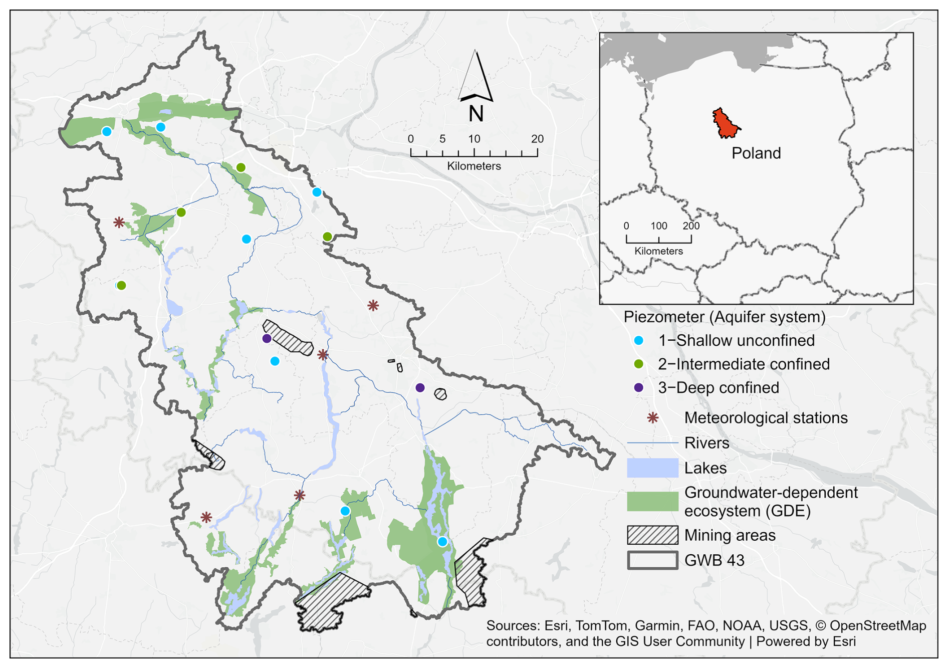
Figure 1 Study area and monitoring network within GWB 43. Location of GWB 43 (PLGW600043) in central-western Poland and spatial distribution of monitoring piezometers grouped into three aquifer systems. The figure includes hydrographic features, lakes, groundwater-dependent ecosystems (GDEs), and mining areas used in the spatial drought-impact framework. Basemap sources: Esri, TomTom, Garmin, FAO, NOAA, USGS, OpenStreetMap contributors, and the GIS User Community | Powered by Esri.

2.2 Hydrogeological framework

GWB 43 comprises three principal aquifer systems: (1) shallow Quaternary sands and gravels, (2) Neogene–Paleogene sandy formations associated with lignite-bearing sequences, and (3) locally fractured Upper Cretaceous carbonates. Recharge of the shallow system occurs mainly through direct infiltration of precipitation, whereas the deeper aquifers are replenished by leakage through discontinuous clay layers and via hydraulic windows. Strong vertical connectivity between aquifers has been documented in several zones, particularly where mining drainage or river valleys modify the hydraulic gradient. This structural configuration results in a system that is sensitive to both climatic forcing and anthropogenic drainage (PGI-NRI, 2022).

Since 2012, national assessments have consistently classified GWB 43 as having poor quantitative and chemical status. Exceedances most often involve nitrate, ammonium, sulfate, and sodium, reflecting the combined impact of agricultural runoff, inadequate rural sanitation, and possible upconing of mineralized waters from deeper layers. Many monitoring wells lack protective low-permeability covers, further increasing their vulnerability to pollution and speeding up the transfer of surface signals into groundwater (The Polish Geological Institute – National Research Institute, 2022). These features are illustrated in the conceptual cross-section (Fig. 2).

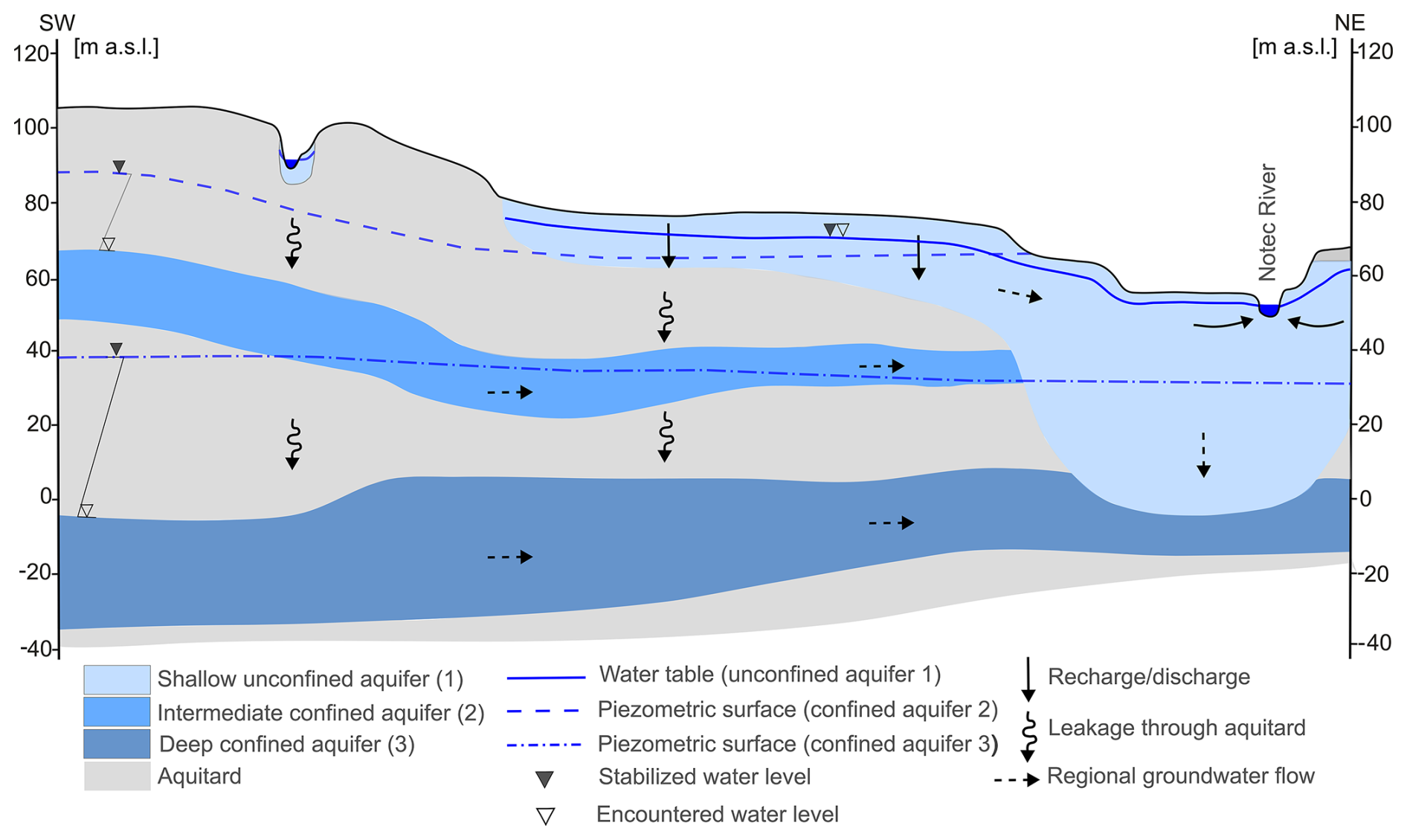
Figure 2 Conceptual hydrogeological cross-section of the GWB 43 aquifer system. Conceptual SW–NE cross-section illustrating the three principal aquifer systems in GWB 43: shallow unconfined, intermediate confined, and deep confined aquifers. The scheme highlights vertical hydraulic connectivity, leakage through aquitards, recharge/discharge zones, and dominant regional groundwater-flow directions that underpin differences in drought propagation and recovery.

2.3 Anthropogenic pressures on groundwater systems

The groundwater system within GWB 43 faces significant human-induced stress from both groundwater extraction and mining activities. Based on available data, a total of 1267 groundwater-related features were identified in the study area, including 1247 abstraction wells and 20 dewatering wells linked to mining operations. The spatial distribution of groundwater abstractions and mining activities, along with the normalised pressure layers used in the DIPI framework, is shown in Appendix A (Fig. A1).

Groundwater abstraction is widespread and includes a range of uses, such as municipal water supply, agricultural abstraction, and individual wells serving local infrastructure (e.g., schools, healthcare facilities, and dispersed settlements). The spatial distribution of these wells is heterogeneous, with locally high densities reflecting areas of intensified water use.

In addition to abstraction, groundwater conditions are influenced by mining-related dewatering associated with open-pit operations. These activities generate local-to-regional-scale depression cones and modify hydraulic gradients, thereby affecting groundwater flow patterns and storage conditions (Fiszer and Derkowska-Sitarz, 2010; Przybyłek, 2018; Nowak et al., 2023).

The coexistence of widespread groundwater abstraction and localized high-intensity dewatering results in a complex pattern of anthropogenic pressure superimposed on natural hydrogeological conditions. This makes GWB 43 a representative example of a groundwater system where climatic forcing interacts with substantial human pressure, providing a suitable framework for analyzing the combined effects of system response and external stressors on groundwater drought dynamics.

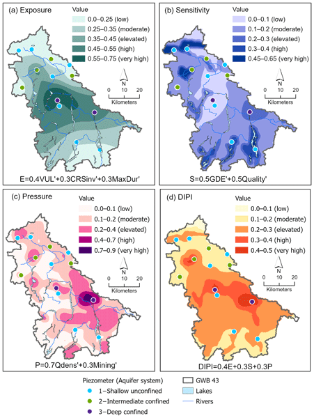
The spatial distribution of these anthropogenic pressures is synthesized in the pressure component (P) and presented as a continuous surface in Fig. 7, forming one of the key inputs to the DIPI framework.

3 Datasets

This study integrates groundwater-level, groundwater-chemistry, and precipitation datasets for the GWB 43 groundwater body. The objective was to characterize groundwater drought dynamics consistently across aquifer levels and to compare them with meteorological forcing.

3.1 Precipitation

Monthly precipitation totals were obtained from five meteorological stations operated by the Institute of Meteorology and Water Management – National Research Institute (IMGW-PIB): Gębice, Zalesie, Trzemeszno, Pakość and Jaksice. Continuous records covering 1986–2024 were used to compute the Standardized Precipitation Index (SPI) at monthly resolution, consistent with SGI calculations.

3.2 Groundwater

Groundwater-level records were obtained from the national monitoring network operated by the Polish Geological Institute – National Research Institute (Państwowy Instytut Geologiczny – Państwowy Instytut Badawczy; PIG-PIB) under the State Hydrogeological Service (Państwowa Służba Hydrogeologiczna; PSH), and by the Chief Inspectorate of Environmental Protection (Główny Inspektorat Ochrony Środowiska; GIOŚ) within the State Environmental Monitoring program (Państwowy Monitoring Środowiska; PMŚ). The hydrogeological and meteorological time series used in this study were partly derived from raw datasets compiled in an earlier MS thesis focused on a preliminary groundwater drought assessment in GWB 43 (Jurzyk, 2025). In the present study, however, these input data were reprocessed within a substantially revised analytical framework, including a new expert-based piezometer classification, expanded event-based drought metrics, and the development of the Drought Impact Potential Index (DIPI). Sixteen monitoring wells within GWB 43 were selected and assigned to three hydrostratigraphic groups: unconfined, intermediate, and deep confined aquifers. Hydraulic heads were converted to monthly means and used to compute the Standardized Groundwater Level Index (SGI).

Observation periods differed among piezometers, and several records contained missing months. The complete start and end dates, number of valid monthly observations, and data completeness for each piezometer are provided in Table 1. Missing groundwater-level observations were not interpolated. For each piezometer, trailing 3-, 6-, and 12-month aggregation windows were calculated only when all constituent calendar months were available. Consequently, the SGI series differ slightly in length among wells and aggregation scales. Key characteristics of the groundwater monitoring wells aggregated by aquifer type are summarised in Table 1.

Table 1 Characteristics of monitoring piezometers grouped by aquifer system in GWB 43.

Notes: Screen interval denotes the top and bottom of the monitored interval below ground level. Observation period is reported separately for each piezometer and spans the first to the last valid monthly observation. Completeness was calculated as the ratio of valid monthly observations to the expected number of months within the reported period. Missing groundwater-level observations were not interpolated.

The assignment of piezometers to three hydrogeological groups was defined a priori, based on stratigraphic position, confinement conditions, and typical groundwater-table depth. These groups represent three conceptually distinct groundwater systems: shallow unconfined, intermediate confined, and deep confined aquifers. The consistency of SGI responses across the three aggregation scales supports the interpretation that the observed differences reflect contrasts in storage and recharge connectivity rather than solely effects of temporal averaging.

Since the grouping is expert-based rather than statistical analysis, and the number of observation wells in confined horizons is limited (4 and 2 wells, respectively), the results should be viewed as characteristic of typical settings rather than as population-wide statistics for the entire aquifer. This limitation is somewhat offset by the internal consistency of SGI metrics across different indices and by agreement with the conceptual hydrogeological model. Future work should evaluate the stability of these groups with additional monitoring points and, where possible, use complementary statistical grouping methods.

Aquifer-group mean SGI series were calculated as the arithmetic mean of the available well-level SGI values for each month. To reduce changes in temporal network support, a monthly aquifer-group mean was calculated only when data were available from at least 50 % of the wells assigned to that group and from at least two wells. This required a minimum of five wells for the shallow unconfined aquifer, two wells for the intermediate confined aquifer, and both wells for the deep confined aquifer. The number of wells contributing to each monthly mean was also recorded.

4 Methods

The conceptual model highlights differences in damping, lag, and memory effects, which are quantified using the drought metrics described below (Fig. 3).

Figure 3 Conceptual model of groundwater drought propagation and recovery across aquifer systems. Schematic representation of SPI–SGI response behaviour across groundwater systems of increasing depth and memory. Dashed lines indicate meteorological forcing (SPI), whereas solid lines represent groundwater response (SGI): (a) rapid propagation in the shallow unconfined aquifer, (b) attenuated and delayed response in the intermediate confined aquifer, and (c) threshold-like response in the deep confined aquifer.

4.1 Standardized Precipitation Index (SPI)

The Standardized Precipitation Index (SPI) was used to quantify meteorological drought at multiple time scales. SPI expresses the deviation of precipitation from the long-term climatology in units of standard deviation, allowing comparison between stations and regions with different climates (McKee et al., 1993; Guttman, 1999; WMO, 2012).

SPI was used as a consistent indicator of precipitation deficit rather than as a complete representation of climatic water balance or effective groundwater recharge. It does not explicitly account for potential or actual evapotranspiration, temperature, soil-moisture dynamics, snow processes, or the timing and magnitude of recharge.

Monthly precipitation totals from the five IMGW-PIB stations were first aggregated to 3-, 6-, and 12-month moving sums to represent short-term, seasonal, and annual-scale water balance conditions, respectively. The cumulative distribution function G(P_k) was then transformed to the standard normal distribution:

$$\begin{array}{}\text{(1)}& \mathrm{SPI}={\mathrm{\Phi }}^{-\mathrm{1}}\left(G\left(P_k\right)\right),\end{array}$$

where Φ⁻¹ is the inverse standard normal cumulative distribution function.

Drought conditions were defined using commonly applied SPI thresholds (McKee et al., 1993; WMO, 2012). In this study, we adopt: SPI < −1.0 moderate drought, SPI < −1.5 severe drought, SPI < −2.0 extreme drought.

For each time scale, drought events were identified as continuous periods during which SPI remained below a given threshold. For every event, we computed the duration (number of months), the minimum SPI value, and the accumulated severity (sum of SPI values below the threshold). These metrics were later compared with groundwater drought characteristics derived from SGI.

4.2 Standardized Groundwater Level Index (SGI)

SGI was calculated separately for each piezometer and aggregation scale. Monthly groundwater levels were first aggregated using trailing 3-, 6-, and 12-month arithmetic means. An aggregation window was retained only when all constituent monthly observations were available; missing groundwater-level values were not interpolated.

To remove seasonality, the aggregated groundwater-level values were transformed separately for each calendar month using a non-parametric normal-score transformation:

$$\begin{array}{}\text{(2)}& {\mathrm{SGI}}_{m,i}={\mathit{\varphi }}^{-\mathrm{1}}\left({\displaystyle \frac{r_{m,i}-\mathrm{0.5}}{n_m}}\right),\end{array}$$

where r_m,i is the rank of observation i among all available aggregated values for calendar month m, n_m is the number of valid observations for that month, and Φ⁻¹ is the inverse standard normal cumulative distribution function. Average ranks were used for tied observations.

Drought conditions were defined as SGI < −1, with severity classes analogous to those used for SPI (Hisdal et al., 2000; Tallaksen and Van Lanen, 2004). A drought event consisted of consecutive valid months below this threshold. A gap in the SGI series terminated an ongoing event. SGI describes standardized groundwater-level anomalies but does not independently identify their cause. In the human-modified GWB 43 system, negative SGI values may reflect the combined influence of meteorological drought, aquifer memory, groundwater abstraction, mining-related dewatering, and induced vertical leakage.

Both SPI and SGI were analysed at consistent temporal scales to enable direct comparison of meteorological and groundwater drought dynamics (aggregation periods of 3, 6, and 12 months). Continuous periods below a given threshold were identified as drought events and summarised using standard drought metrics (see Sect. 4.3).

For aquifer-system analyses, aquifer-group mean SGI series were calculated as described in Sect. 3.2 and were used to derive drought metrics for comparison among the monitored aquifer systems.

Part of the raw groundwater-level and meteorological time series used in this study had previously been compiled within an earlier MS thesis study of groundwater drought in GWB 43 (Jurzyk, 2025). However, in the present study, all input data were reprocessed within a substantially revised analytical framework, including a new expert-based piezometer classification, expanded event-based drought metrics, and the development of the Drought Impact Potential Index (DIPI). The methodological steps applied to derive these drought-response metrics and the final index are described in the following section.

4.3 Drought metrics

Based on the reprocessed monthly SGI-12 time series and the updated piezometer grouping, a set of event-based drought metrics was calculated to quantify groundwater system response, including vulnerability, maximum drought duration, resistance, resilience, propagation probability, and median recovery time. Drought events were defined as continuous periods with SGI < −1.0, and a set of metrics describing duration, severity, propagation and recovery was derived following established approaches (Van Loon, 2015; Peters et al., 2003; Thomas and Famiglietti, 2017). Drought metrics were calculated for both individual piezometer SGI series and aquifer-group mean SGI series. The well-level metrics were used as inputs to the spatial Exposure analysis, whereas the group-level metrics were used to compare temporal drought behaviour among aquifer systems.

The full set of applied drought metrics, together with their definitions and calculation formulas, is summarised in Table 2.

Table 2 Definitions and formulas of event-based groundwater drought metrics derived from SGI.

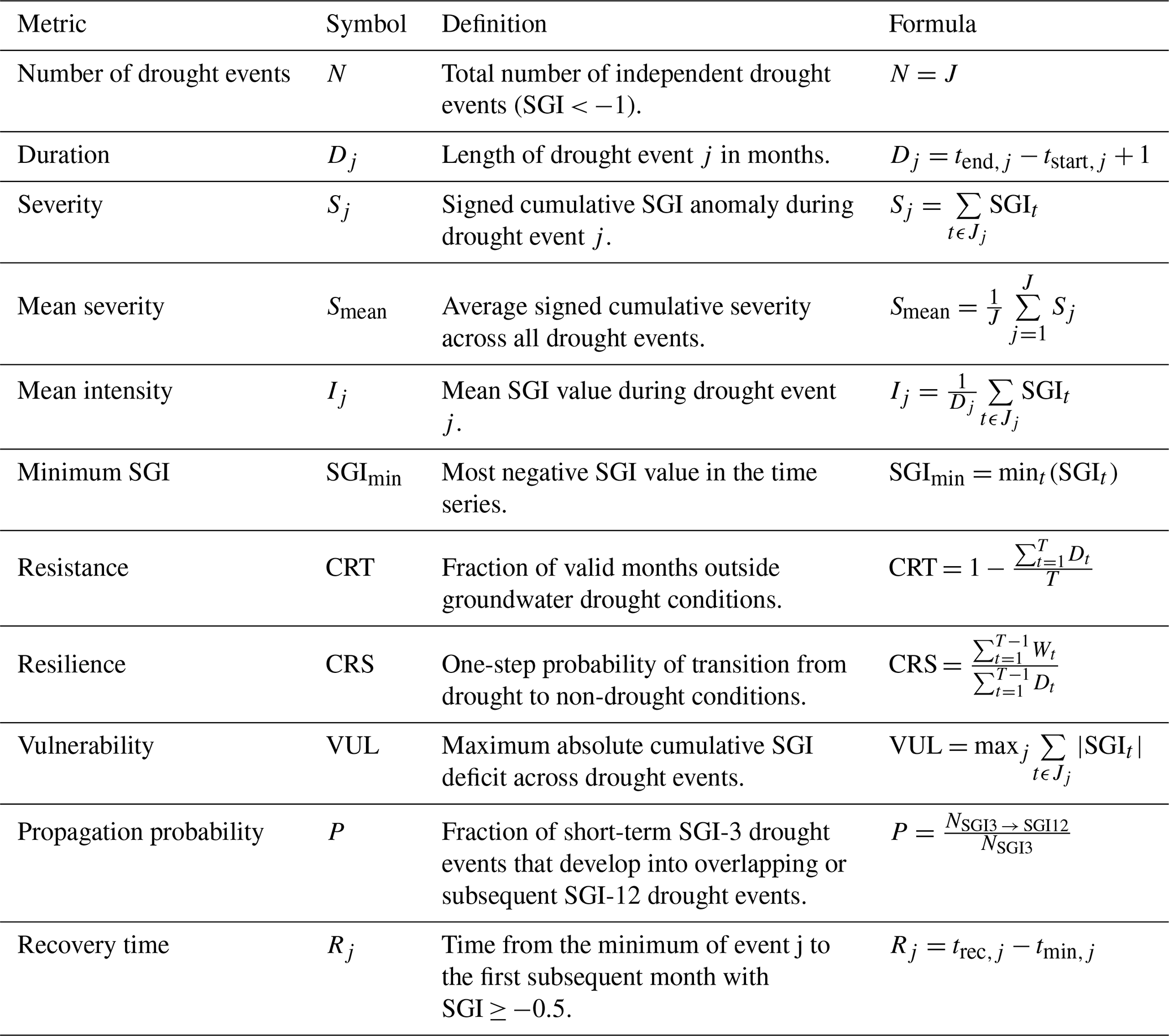
Notes: SGI_t – Standardized Groundwater Level Index at time t; t – time step (month); J – total number of drought events; J_j – set of time steps belonging to drought event j; t_start,j and t_end,j – start and end of event j; t_min,j – time of minimum SGI within event j; t_rec,j – first time step after the event minimum when SGI ≥ −0.5; D_t = 1 if SGI_t < −1 and 0 otherwise; W_t = 1 if D_t = 1 and $D_{t+\mathrm{1}}=\mathrm{0}$, and 0 otherwise; T – total number of valid time steps; NSGI3 – number of short-term SGI-3 groundwater drought events; N_{SGI3 → SGI12} – number of SGI-3 drought events matched to an overlapping or subsequent SGI-12 drought event. Severity is retained as a signed cumulative anomaly and is therefore negative during drought; VUL is reported as a positive absolute cumulative deficit. CRS uses the drought threshold SGI $<-$1, whereas recovery time uses the near-normal threshold SGI ≥ −0.5.

The selected metrics collectively describe both the temporal characteristics of drought events and the dynamic response of groundwater systems, forming the basis for the exposure component of the Drought Impact Potential Index (DIPI) framework.

Statistical analyses, SGI-based drought metrics, and time-series figures were produced in Python within the Google Colab environment using custom scripts. Spatial interpolation, raster processing, and map production were performed in ArcGIS Pro.

4.4 Lagged SPI–SGI correlation analysis

To examine the temporal association between meteorological and groundwater drought, we analysed the relationship between the Standardized Precipitation Index (SPI) and aquifer-group mean Standardized Groundwater Level Index (SGI) series at 3-, 6-, and 12-month aggregation scales, while accounting for delayed groundwater response (Bloomfield and Marchant, 2013; Barker et al., 2016; Kumar et al., 2016). For each monitored aquifer system, SPI was obtained from the precipitation station nearest to the centroid of the corresponding piezometer group. This approach was intended to retain local precipitation variability relevant to groundwater recharge that might be obscured by spatial averaging.

For each station–aquifer-group pair and aggregation scale k, the contemporaneous Pearson correlation coefficient was calculated as:

$$\begin{array}{}\text{(3)}& r_k\left(\mathrm{0}\right)=\mathrm{corr}\left[{\mathrm{SPI}}_k\left(t\right),{\mathrm{SGI}}_k\left(t\right)\right]\end{array}$$

where k=3, 6, or 12 months.

Lagged correlations were then calculated by shifting SGI relative to SPI over lags L=0–12 months:

$$\begin{array}{}\text{(4)}& r_k\left(L\right)=\mathrm{corr}\left[{\mathrm{SPI}}_k\left(t\right),{\mathrm{SGI}}_k\left(t+L\right)\right],\end{array}$$

A positive value of L indicates that the groundwater signal follows the meteorological signal. Only temporally overlapping, non-missing SPI–SGI pairs were included in each correlation calculation.

For each aquifer system and aggregation scale, the lag associated with the highest positive Pearson correlation within the tested 0–12-month range was identified. Similar maximum-correlation approaches have been widely used to characterize the dominant temporal association between meteorological and groundwater drought indices, although the resulting optimal temporal association may vary among sites, aggregation scales, and hydrogeological settings (Bloomfield and Marchant, 2013; Kumar et al., 2016). The identified lag was therefore interpreted as an empirical indicator of the strongest temporal association, rather than as a uniquely determined physical propagation time or a fixed aquifer response time. A maximum at L=12 months indicates that the strongest correlation was found at the upper boundary of the tested range and does not rule out a longer response delay.

To assess whether the identified correlation maxima were stable over time, the lag analysis was repeated within moving 10-year windows, each shifted forward by 1 year. Within each window, Pearson correlations were calculated for lags of 0–12 months, and the lag associated with the maximum positive correlation was recorded. Only windows containing at least 96 valid paired monthly observations were retained. The moving-window analysis was used as a diagnostic sensitivity test of temporal stability, recognizing that the lag associated with the maximum correlation may vary among subperiods and may be influenced by serial dependence and changing climatic or anthropogenic conditions. It was not interpreted as an independent estimate of aquifer response time or as a formal confidence interval for the lag.

To evaluate sensitivity to long-term co-trending, the full-period analysis was also repeated using detrended SPI and SGI series. Interpretation was based on the consistency of the general correlation and lag patterns between the original and detrended series. The complete full-period correlation matrices are presented in Appendix B, whereas the moving-window stability analysis is shown in Appendix C, Fig. C1.

4.5 Spatial analysis and Drought Impact Potential Index (DIPI)

This section represents the core methodological contribution of the study. To assess the spatial distribution of drought impact potential within GWB 43, we developed a composite Drought Impact Potential Index (DIPI) integrating exposure to groundwater drought, anthropogenic pressure, and system sensitivity. This approach is inspired by multidimensional and spatially explicit drought-vulnerability indices that integrate normalized environmental and anthropogenic indicators (Saha et al., 2021; Ling et al., 2023), and is adapted here to hydrogeological conditions.

DIPI was developed as an exploratory spatial screening index intended to compare relative patterns within the study area. The selected component weights reflect expert judgment and were not calibrated against independent observations of groundwater-drought impacts.

For temporal comparison among aquifer systems, SGI series and drought metrics were summarized at the aquifer-group level. In contrast, the spatial Exposure analysis was based on drought metrics calculated independently for each of the 16 monitoring piezometers. Group-level metric values were not assigned to individual wells. For each piezometer, SGI-12 vulnerability (VUL), inverse resilience score (CRS_inv), and maximum drought duration (MaxDur) were calculated from its individual SGI-12 series. These well-level metrics were normalised across the monitoring network and interpolated separately within the GWB 43 boundary. The resulting continuous surfaces were subsequently combined according to the Exposure equation.

The piezometer-level SGI-12 metrics were interpolated separately using the Topo to Raster algorithm, with drainage enforcement disabled. Topo to Raster is based on an iterative finite-difference interpolation procedure related to a discretized thin-plate spline and was used here to generate continuous, smoothed surfaces from irregularly distributed monitoring points (Hutchinson, 1989). The same study-area boundary, raster extent, cell size, and snap raster were applied to all Exposure subcomponents to ensure spatial consistency among the resulting layers.

Interpolation performance was evaluated using leave-one-out cross-validation, a commonly used approach for assessing spatial interpolation accuracy when an independent validation dataset is unavailable (Li and Heap, 2008; Risk et al., 2022). Cross-validation was performed separately for normalized vulnerability (VUL^′), inverse normalized resilience (CRS${}_{\mathrm{inv}}^{\prime }$), and normalized maximum drought duration (MaxDur^′). In each iteration, one of the 16 piezometers was omitted, the interpolation surface was regenerated from the remaining 15 wells using identical settings, and the predicted value was extracted at the location of the omitted piezometer.

Predictive performance was summarized using mean error (ME), mean absolute error (MAE), root mean square error (RMSE), and the Pearson correlation coefficient between observed and predicted values. To further assess the sensitivity of the spatial results to monitoring-network configuration, the existing leave-one-out results were used for an additional network-influence diagnostic. For each piezometer, interpolation errors were compared across the three Exposure subcomponents, and the proportion of the total absolute and squared error attributable to individual monitoring locations was quantified. In addition, local metric contrast was represented by the absolute difference in observed metric values between each piezometer and its nearest neighbouring monitoring point, and its association with absolute LOOCV error was evaluated using Pearson and Spearman correlations. This diagnostic was used to identify whether interpolation uncertainty was broadly distributed across the network or concentrated at locally contrasting or poorly represented monitoring locations. The resulting network-influence diagnostics are summarized in Table D1.

ME was used to assess overall directional bias, whereas MAE and RMSE quantified the magnitude of prediction errors; both measures were retained because they emphasize different characteristics of the error distribution (Willmott and Matsuura, 2006). Detailed observed, predicted, and error values are provided in the reproducibility package.

Interpolation was constrained within the GWB 43 boundary to prevent artifacts outside the study area (e.g., Goovaerts, 1997; Hengl, 2009). We focus on metrics derived from the 12-month Standardized Groundwater Index (SGI-12) because multi-year aggregations better reflect long-term groundwater drought persistence and have stronger relationships with hydrological impacts compared to shorter windows (Bloomfield and Marchant, 2013; Kumar et al., 2016).

The Drought Impact Potential Index (DIPI) is defined as a weighted sum of three components: Exposure (E), Pressure (P), and Sensitivity (S). The weights determine the relative contribution of the normalised Exposure, Pressure, and Sensitivity components to the composite DIPI score (e.g., Wheater and Evans, 2009; Porter et al., 2014).

All components and sub-components were normalised using min–max scaling prior to aggregation, as shown in Table 3.

Table 3 Components, sub-components, and aggregation equations of the Drought Impact Potential Index (DIPI).

Notes: Variables marked with a prime (^′) denote dimensionless values normalised to the interval [0, 1] using min–max scaling. CRSinv^′ is the inverse min–max-normalised resilience score; higher values therefore indicate lower resilience and higher relative Exposure. Mining^′, GDE^′, and Quality^′ are spatially derived indicators normalised to the range 0–1. All Exposure sub-components were calculated independently for each piezometer from SGI-12 metrics and interpolated separately before aggregation. The Pressure component assigns a weight of 0.7 to abstraction density and 0.3 to mining influence, whereas the two Sensitivity sub-components are equally weighted. The final DIPI uses expert-based weights of 0.4 for Exposure, 0.3 for Pressure, and 0.3 for Sensitivity. All component and composite scores are relative, dimensionless screening indicators and should not be interpreted as absolute probabilities or impact magnitudes.

The expert-based weights were used for exploratory spatial screening and were not calibrated against an independent impact dataset. Final DIPI values are mapped using continuous surfaces (interpolated from piezometer measurements) and classified into quantiles for cartographic visualization. The full spatial representation of all normalised sub-components and both DIPI aggregation schemes is provided in Appendix A (Fig. A1) to ensure methodological transparency and reproducibility of the framework. All intermediate datasets, reproducible notebooks, and figure source tables are openly archived in Zenodo (Sawicka and Jurzyk, 2026).

A spatial contrast index was calculated as the difference between the normalised Exposure and Pressure components (E−P). The index was used as a descriptive comparison of their relative mapped magnitudes and not as a causal attribution metric.

5 Results

5.1 Standardized Precipitation Index (SPI)

The temporal evolution of the SPI calculated for 3-, 6-, and 12-month aggregation windows reveals a largely coherent drought signal across the five precipitation stations. Although individual stations show some differences in amplitude, most drought episodes occur synchronously, indicating regionally consistent atmospheric forcing.

For SPI-3, several short and intense droughts are evident, with minima below −3 at most stations. At the 6-month scale, droughts become less abrupt but more persistent, with the most significant regional event in 2003, when the areal mean dropped to −2.93. The 12-month SPI emphasizes the multi-year nature of this episode, with the lowest areal value of −2.69 recorded in late 2003.

Overall, the mean SPI closely tracks individual stations, confirming that major drought episodes were spatially widespread rather than localized.

5.2 Standardized Groundwater Level Index (SGI)

The SGI calculated for 3-, 6-, and 12-month aggregation windows reveals clear differences among the monitored aquifer systems in the timing, magnitude, and persistence of groundwater droughts (Fig. 4). The shallow unconfined aquifer generally showed shorter and less severe anomalies, whereas the deep confined aquifer displayed the most persistent deficits.

Figure 4 Temporal variation in SGI across aquifer systems and aggregation timescales in GWB 43. Mean SGI-3, SGI-6, and SGI-12 time series for the three aquifer systems: (a) shallow unconfined, (b) intermediate confined, and (c) deep confined. The dashed horizontal line marks the groundwater-drought threshold (SGI $=-\mathrm{1}$). Grey shading indicates meteorological drought periods, defined as months in which the spatially averaged SPI-3, SPI-6, or SPI-12 was below −1.

At the SGI-3 scale, the minimum values were −1.34 in the shallow unconfined aquifer in September 2023, −1.87 in the intermediate confined aquifer in June 2016, and −2.15 in the deep confined aquifer in September 2023. The shallow system experienced several relatively short drought episodes, including events in 2015–2016 and 2023. In the intermediate system, the most pronounced short-term event occurred in 2015–2016, followed by additional deficits in 2019–2020 and 2022–2023. In contrast, the deep aquifer showed prolonged SGI-3 droughts, including a 19-month event in 2019–2021 and a 23-month event extending from May 2022 to March 2024.

At the SGI-6 scale, the minima were −1.27, −1.72, and −2.15 for the shallow, intermediate, and deep systems, respectively. Increasing the aggregation window smoothed short-term variability and increased drought persistence, particularly in the deep aquifer. In the deep confined aquifer, one SGI-6 drought event lasted 36 months during 2019–2022, while a subsequent event lasted 22 months from June 2022 to March 2024 (Fig. 4).

The contrast among the systems was most apparent at the SGI-12 scale. The shallow and intermediate aquifers reached minima of −1.19 and −1.57, respectively, and their drought episodes generally lasted between 5 and 10 months. In the deep confined aquifer, SGI-12 remained below −1 from August 2019 until the end of the available record in March 2024, forming a 56-month event with a minimum of −1.87. This prolonged anomaly indicates a persistent depletion signal in the monitored deep system, although its interpretation must account for the limited number of deep-aquifer wells and the possible influence of sustained anthropogenic pressure.

As shown in Appendix B (Fig. B1), the shallow unconfined aquifer exhibited the strongest full-period SPI–SGI associations. Maximum correlations were r=0.32 for SGI-3, r=0.491 for SGI-6, and r=0.651 for SGI-12, all at a lag of 9 months.

The intermediate confined aquifer showed weaker and less uniform associations. Maximum correlations were r=0.272 at a lag of 2 months for SGI-3, r=0.325 at 5 months for SGI-6, and r=0.281 at 6 months for SGI-12.

In the deep confined aquifer, maximum correlations were r=0.184, r=0.303, and r=0.380 for SGI-3, SGI-6, and SGI-12, respectively. All maxima occurred at the upper tested lag of 12 months, indicating that the strongest association may occur beyond the analysed range and cannot be resolved precisely.

Overall, the full-period results indicate the strongest and most coherent meteorological association in the shallow unconfined aquifer and a progressively delayed relationship in the deep confined aquifer. However, the moving-window analysis showed that the lag associated with the maximum correlation varied among subperiods (Appendix C, Fig. C1). The reported lags should therefore be interpreted as empirical indicators of temporal association within the tested range rather than as fixed aquifer-response times or direct evidence of a propagation mechanism.

The moving-window analysis showed that the lag associated with the maximum SPI–SGI correlation was not fully stationary through time (Appendix C, Fig. C1). In the shallow unconfined aquifer, the SGI-12 maximum was comparatively stable and generally occurred at lags of 7–10 months, most frequently at 9 months. The intermediate confined aquifer showed relatively stable maxima for SGI-6 and SGI-12, whereas the SGI-3 lag varied more strongly among subperiods. In the deep confined aquifer, maximum correlations most frequently occurred near the upper boundary of the tested range, particularly for SGI-6 and SGI-12.

5.3 Drought metrics

Groundwater drought characteristics derived from the SGI series show clear differences among aquifer groups and aggregation scales (Table 4; Fig. 5). At the 3-month scale, drought events were shortest in the shallow and intermediate aquifers. The shallow unconfined aquifer experienced five events with a mean duration of 4.0 months and a maximum duration of 7 months, whereas the intermediate confined aquifer experienced eight events with a mean duration of 5.1 months and a maximum duration of 10 months. The deep confined aquifer showed substantially longer and more severe droughts, with a mean duration of 11.8 months, a maximum duration of 23 months, and a mean cumulative severity of −16.96.

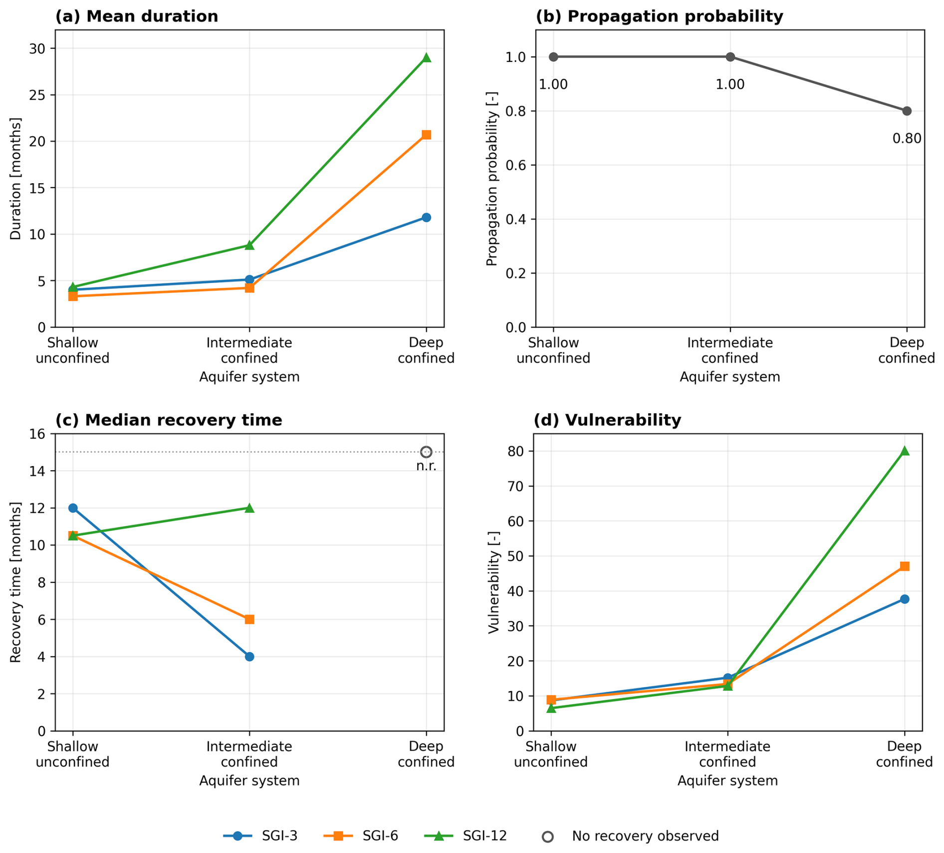
Figure 5 Groundwater drought metrics across the three monitored aquifer systems and aggregation scales. Comparison of (a) mean drought duration, (b) propagation probability from SGI-3 to SGI-12, (c) median recovery time, and (d) vulnerability (VUL) for the shallow unconfined, intermediate confined, and deep confined aquifer systems. Mean duration, recovery time, and vulnerability are shown for SGI-3, SGI-6, and SGI-12. Propagation probability is reported as a single SGI-3-to-SGI-12 value for each aquifer system. Open symbols and “n.r.” indicate that no recovery was observed within the available monitoring period.

At the 6-month scale, droughts in the shallow unconfined and intermediate confined aquifers remained comparatively short, with mean durations of 3.3 and 4.2 months, respectively. In contrast, the deep confined aquifer experienced only three events, but their mean duration increased to 20.7 months, and the longest event lasted 36 months. The corresponding vulnerability value (VUL) increased to 47.02, compared with 8.87 and 13.38 in the shallow unconfined and intermediate confined aquifers. At the 12-month scale, the contrast between the deep aquifer and the two shallower systems remained pronounced. The shallow unconfined aquifer experienced four events with a mean duration of 4.3 months, whereas the intermediate confined aquifer experienced five events with a mean duration of 8.8 months. The deep confined aquifer experienced two long-term events with a mean duration of 29 months and a maximum duration of 56 months. It also had the highest cumulative severity (−41.09) and vulnerability (VUL =80.10).

Resistance (CRT), defined as the fraction of valid months outside groundwater drought, ranged from 0.815 to 0.918. The lowest values occurred in the deep confined aquifer, indicating a larger proportion of months affected by drought. Resilience (CRS), defined as the probability of transition from drought to non-drought conditions, was also lowest in the deep confined aquifer and declined from 0.069 at SGI-3 to 0.018 at SGI-12.

Recovery was observed for all SGI-3 and SGI-6 events in shallow and intermediate aquifers. Median recovery times ranged from 4 to 12 months. At SGI-12, two of four events in the shallow unconfined aquifer recovered, with a median recovery time of 10.5 months, whereas all five events in the intermediate confined aquifer recovered within a median of 12 months. No recovery was observed for any event in the deep confined aquifer within the available observation period.

Across the monitored aquifer systems, the deep confined aquifer exhibited the longest and most persistent drought episodes. Because it is represented by only two wells, this contrast should be interpreted as characteristic of the monitored locations rather than as a general depth-dependent relationship.

Table 4 Groundwater drought metrics derived from aquifer-group mean SGI series at 3-, 6-, and 12-month aggregation scales.

Notes: Propagation probability is defined only for the transition from SGI-3 to SGI-12 and is therefore reported in the SGI-3 rows. Recovery denotes the median number of months from the event minimum to the first month with SGI ≥ −0.5. CRT is the fraction of valid months outside drought conditions, whereas CRS is the one-step probability of transition from drought to non-drought. VUL is the maximum cumulative positive SGI deficit. Recovered and unrecovered events indicate the number of events for which recovery was or was not observed. Mean severity is expressed as the signed mean cumulative SGI severity; negative values indicate groundwater deficit. Propagation probability denotes the fraction of SGI-3 events matched to an SGI-12 event. For the shallow unconfined aquifer at SGI-12, the median recovery time of 10.5 months is based on two recovered events; two additional events did not recover within the available record. n.r. – no recovery observed; – not applicable.

Figure 5 shows systematic differences in drought patterns across groundwater systems. Duration and vulnerability were highest in the monitored deep confined aquifer, whereas propagation probability showed less systematic variation among aquifer systems. At SGI-12, recovery time could not be estimated for the deep confined aquifer because no recovery was observed within the available record.

5.4 Groundwater drought propagation and recovery

Propagation probability was defined as the fraction of SGI-3 drought events that could be matched to a subsequent or overlapping SGI-12 drought event. Under this definition, all SGI-3 events in the shallow unconfined and intermediate confined aquifers propagated to the 12-month scale, giving propagation probabilities of 1.00. In the deep confined aquifer, four of five SGI-3 events were matched to SGI-12 events, resulting in a propagation probability of 0.80.

These values indicate that the occurrence of a short-term groundwater drought was commonly associated with a longer-term groundwater deficit in all three aquifer systems. However, propagation probability alone did not distinguish the deep aquifer as the most drought-prone system. The strongest contrast among aquifer groups was instead expressed by drought duration, cumulative severity, vulnerability, and recovery behaviour.

The shallow and intermediate aquifers generally showed shorter drought events and more frequent recovery. All SGI-3 and SGI-6 events in the shallow unconfined and intermediate confined aquifers returned to near-normal conditions within the available record. At SGI-12, recovery was observed for all events in the intermediate confined aquifer, whereas two of four events in the shallow unconfined aquifer did not recover before the end of the available series.

The deep confined aquifer displayed a markedly different response. Its drought events were longer and more severe at all aggregation scales, and no event recovered to SGI ≥ −0.5 within the available observation period. The progressive decrease in CRS and the increase in maximum duration and VUL with aggregation scale indicate persistent groundwater deficits and limited short-term recovery.

Because aquifer depth is confounded with geographic location, monitoring-period length, and hydrogeological setting, these differences should not be interpreted as a general depth-dependent relationship. They describe the behaviour of the monitored aquifer groups within GWB 43 and should be viewed as characteristic of these specific hydrogeological settings.

Piezometer-level propagation probabilities ranged from approximately 0.57 to 1.00, indicating substantial within-aquifer-system variability (Fig. 6). These values were calculated independently for individual piezometers and therefore should not be interpreted as deviations around the aquifer-system-level probabilities derived from aquifer-group mean SGI series.

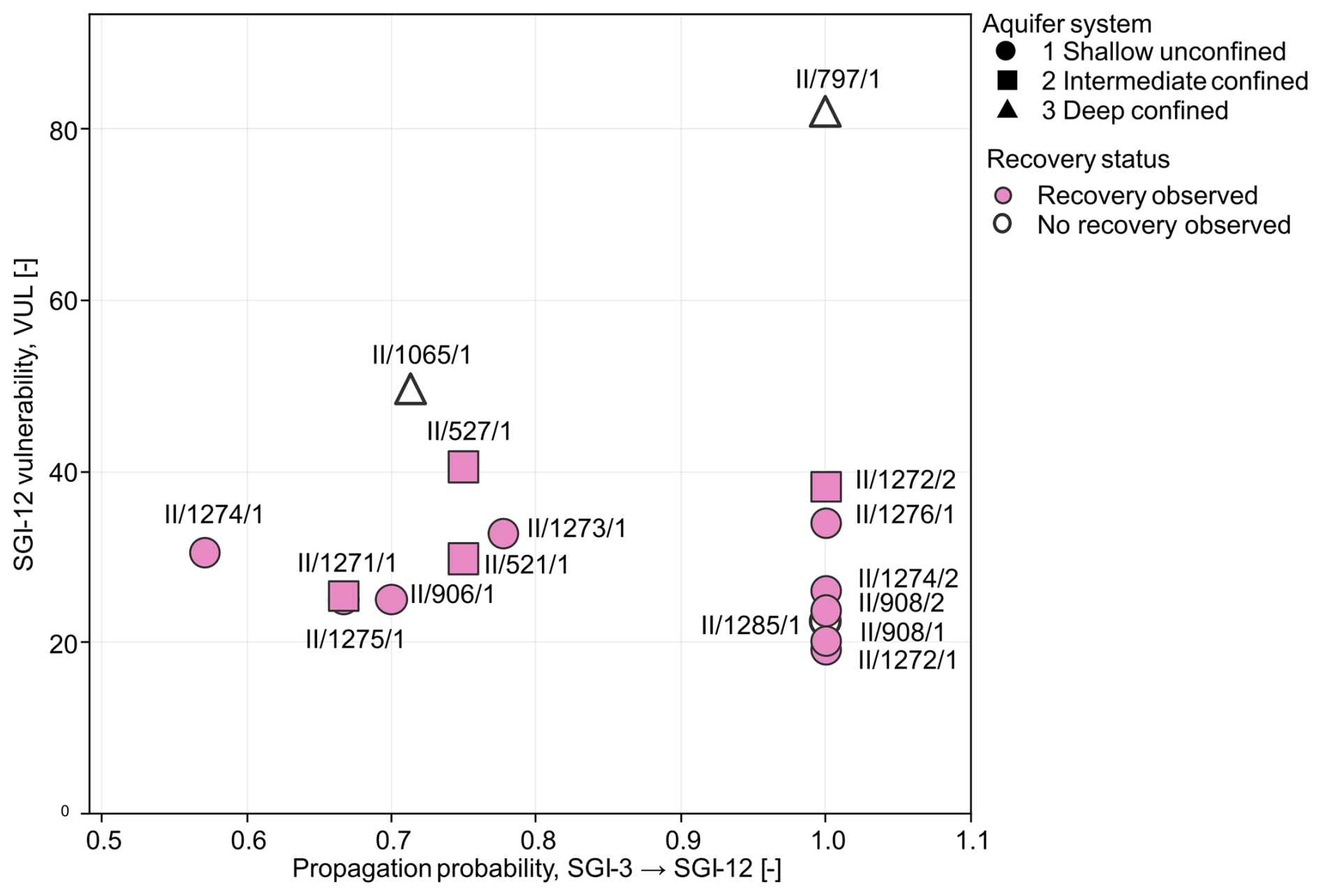
Figure 6 Piezometer-level relationship between groundwater drought propagation and long-term persistence. Propagation probability was calculated independently for each piezometer as the fraction of SGI-3 drought events matched to overlapping or subsequent SGI-12 events. The vertical axis shows piezometer-level SGI-12 vulnerability (VUL), while marker size represents the maximum SGI-12 drought duration. Marker shape identifies the aquifer system, pink-filled symbols indicate that recovery to SGI ≥ −0.5 was observed for at least one event, and open symbols indicate no observed recovery within the available record.

5.5 Drought Impact Potential Index (DIPI)

The mapped DIPI values represent relative spatial scores within GWB 43 and should not be interpreted as absolute probabilities or magnitudes of groundwater drought impact. The revised DIPI was calculated as a weighted combination of Exposure, Pressure, and Sensitivity DIPI $=\mathrm{0.4}E+\mathrm{0.3}P+\mathrm{0.3}S$.

An equally weighted formulation, $(E+P+S)/\mathrm{3}$, was also calculated to examine the sensitivity of the spatial pattern to the adopted component weights.

The weighted and equally weighted formulations produced broadly similar regional patterns, with areas of comparatively higher and lower index values occurring in similar parts of the study area (Fig. 7; Appendix A, Fig. A1). Differences between the two formulations were mainly expressed as local changes in index magnitude and class boundaries. This agreement indicates that the broad spatial pattern is not strongly dependent on the selected weighting scheme. However, it should not be interpreted as evidence that individual mapped values or the boundaries of higher-index areas are spatially robust.

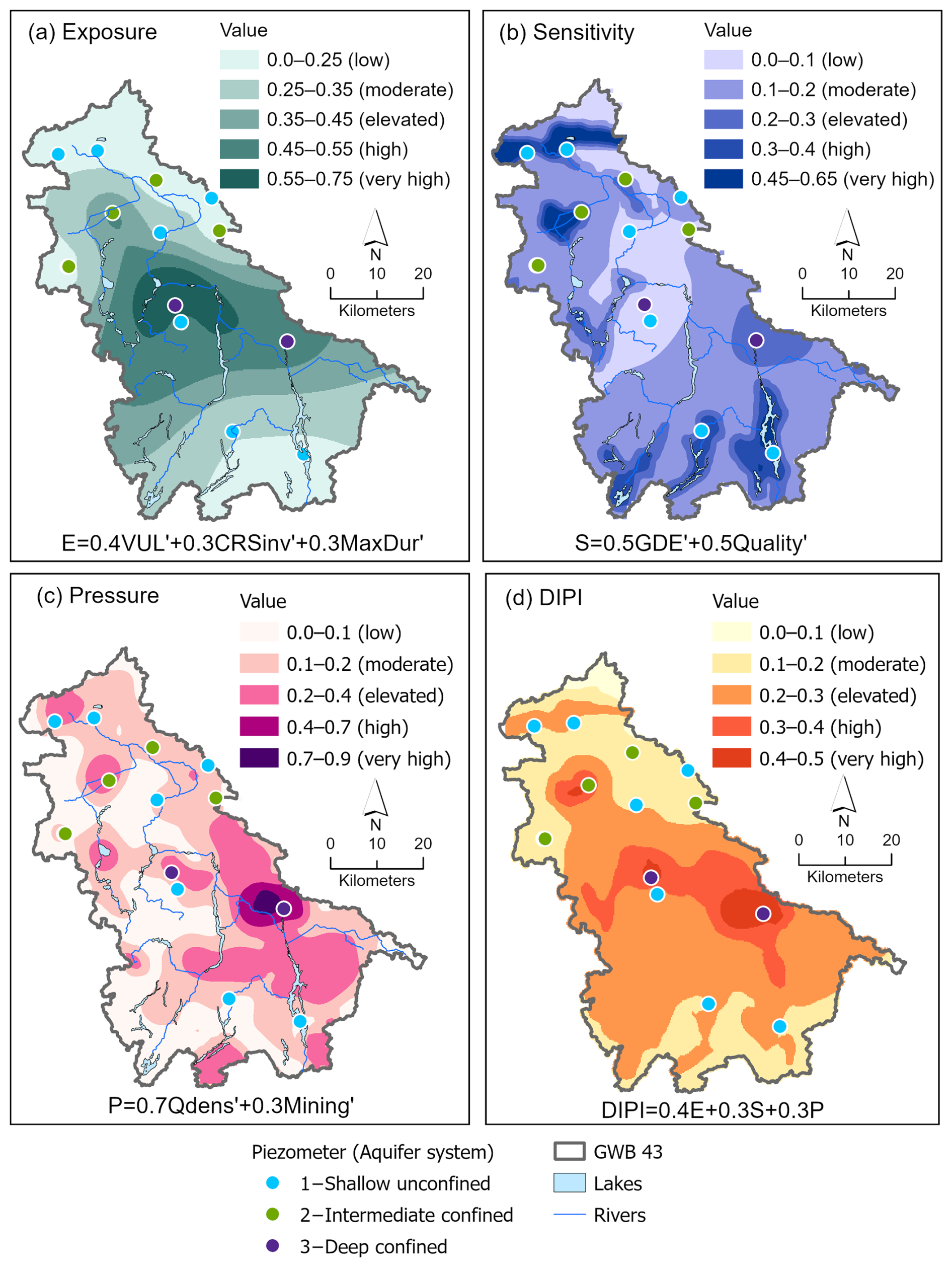
Figure 7 Spatial distribution of DIPI and its component layers in GWB 43. Spatial distribution of the Drought Impact Potential Index (DIPI) and its component layers: (a) Exposure (E), (b) Sensitivity (S), (c) Pressure (P), and (d) final DIPI. Exposure integrates groundwater drought metrics, sensitivity reflects GDE and groundwater-quality constraints, and pressure represents abstraction density and mining-related stress. All components were normalised to the 0–1 range prior to integration.

The weighted DIPI ranged from approximately 0.066 to 0.583. Comparatively higher values occurred mainly in the central and east-central parts of GWB 43, whereas lower values were more common in the northern sector and in parts of the southern area. The resulting surface reflects the combined spatial distribution of groundwater drought Exposure, anthropogenic Pressure, and environmental Sensitivity. It should therefore be interpreted as an exploratory screening representation of relative drought impact potential rather than as a predictive vulnerability map.

Aggregation of DIPI values at piezometer locations showed very similar mean scores for the shallow unconfined and intermediate confined aquifer systems. Under the weighted formulation, mean DIPI was 0.187 for the shallow unconfined aquifer and 0.189 for the intermediate confined aquifer, while the deep confined aquifer reached 0.470. The equal-weight formulation produced corresponding values of 0.194, 0.182, and 0.442. Thus, the distinction between the shallow and intermediate aquifer systems is limited, whereas the deep confined aquifer consistently shows substantially higher relative DIPI values under both weighting schemes. Because the deep confined aquifer is represented by only two piezometers, this contrast should be interpreted cautiously and as indicative rather than spatially representative.

Leave-one-out cross-validation of the three interpolated Exposure subcomponents indicated substantial spatial uncertainty. Across normalised vulnerability, inverse resilience, and maximum drought duration, MAE ranged from 0.211 to 0.287 and RMSE from 0.315 to 0.344. Mean errors were close to zero, indicating limited overall bias, but observed–predicted correlations were weak ($r=-\mathrm{0.195}$ to 0.108). The largest errors occurred in sparsely monitored areas and where spatially adjacent piezometers represented different aquifer systems with contrasting drought-response metrics. These results indicate a limited ability to reproduce local piezometer-scale variability and support the interpretation of the DIPI surface as an exploratory regional screening product.

The network-influence diagnostic showed that interpolation uncertainty was strongly concentrated at a small number of monitoring locations. Two piezometers, II/797/1 and II/1285/1, accounted jointly for 77.8 % of the total squared LOOCV error for VUL^′ and 72.5 % for MaxDur^′, but only 8.1 % for CRS${}_{\mathrm{INV}}^{\prime }$. Local metric contrast was strongly associated with absolute LOOCV error for VUL^′ (Pearson r=0.965) and MaxDur^′ (r=0.963), and more moderately for CRS${}_{\mathrm{INV}}^{\prime }$ (r=0.658). These results indicate that interpolation performance is particularly sensitive to locally contrasting observations and to the hydrostratigraphic representation of the monitoring network, rather than being controlled solely by overall monitoring density (Table D1).

5.6 Exposure–pressure contrast

The spatial contrast between normalised Exposure (E) and Pressure (P), expressed as E−P, was predominantly positive across GWB 43, with localized negative and near-zero zones (Fig. 8). Positive values indicate areas where the mapped Exposure score exceeds the mapped Pressure score, negative values indicate the opposite, and values between −0.1 and 0.1 represent a balanced contrast. Area-based classification showed that E>P covered 65.5 % of the study area, E≈P covered 31.6 %, and E<P covered 2.9 %. These classes describe only the relative mapped magnitudes of the two normalised components and do not provide causal attribution of groundwater-drought controls (Fig. 8).

Figure 8 Spatial contrast between normalised Exposure (E) and Pressure (P) in GWB 43. Positive values indicate areas where E exceeds P, negative values indicate areas where P exceeds E, and values between −0.1 and 0.1 represent a balanced contrast. The E−P classes provide a descriptive comparison of the relative mapped component magnitudes and should not be interpreted as causal attribution.

Spatial contrast between normalised Exposure (E) and Pressure (P) is expressed as E−P. Positive values indicate areas where the normalised Exposure score exceeds the normalised Pressure score, whereas negative values indicate areas where Pressure exceeds Exposure. Values close to zero indicate similar mapped magnitudes of the two components. The contrast is descriptive and does not separate natural and anthropogenic controls.

6 Discussion

The combined analysis of SGI time series, propagation–recovery relationships, and drought metrics indicates contrasting temporal behaviour among the monitored aquifer systems in GWB 43. The shallow unconfined system generally exhibits shorter and less persistent groundwater deficits, whereas the intermediate and deep confined systems show increasingly prolonged anomalies. The persistent signal in the deep aquifer is consistent with greater system memory, although its interpretation remains constrained by the limited number of monitoring wells and the possible influence of sustained anthropogenic pressure.

These results integrate groundwater drought into a hydrogeologically informed statistical framework in which observed system behaviour reflects interactions between external forcing and aquifer characteristics, consistent with recent large-sample groundwater studies (Ebeling et al., 2025).

6.1 System memory and aquifer depth

The observed contrasts are consistent with differences in aquifer memory associated with confinement, storage, and recharge connectivity. The stronger SPI–SGI association in the shallow unconfined aquifer suggests lower attenuation of precipitation variability and closer hydraulic connection with recharge. In the confined systems, greater storage and hydraulic separation may attenuate short-term variability and prolong groundwater-level anomalies. However, these patterns cannot be attributed solely to aquifer depth because monitoring location, record length, hydraulic connectivity, and anthropogenic modification differ among the groups.

This behaviour aligns with previous research emphasizing the importance of aquifer storage and hydraulic connectivity in regulating groundwater memory (Van Loon, 2015; Bloomfield and Marchant, 2013). Recent studies further verify that groundwater response times and memory are heavily influenced by aquifer depth and hydrogeological conditions (Ebeling et al., 2025).

Furthermore, recent studies of the land water cycle show that hydrological memory greatly increases from atmospheric to underground parts, with groundwater showing the strongest persistence and long-term storage effects (Berghuijs et al., 2025).

As a result, deeper and more confined systems display smoother but more persistent drought signals, while shallow systems maintain closer connection with atmospheric forcing. These findings support the interpretation that groundwater drought cannot be viewed simply as a reaction to precipitation anomalies, but must be understood as influenced by aquifer structure and internal system dynamics.

6.2 Propagation and recovery asymmetry

The results indicate an asymmetry between drought development and recovery. Propagation is associated with the accumulation of meteorological deficits, whereas recovery depends on sustained recharge and restoration of groundwater storage. In the monitored deep confined aquifer, drought events were less frequent but more persistent, while the shallow unconfined aquifer generally showed shorter deficits and more frequent recovery.

This asymmetry is especially clear in deeper systems, where droughts happen less often but, once they start, last longer and recover slowly. In contrast, shallow systems show both quick spread and quick recovery, reflecting a more active but less lasting response pattern.

Recent studies increasingly emphasize that drought propagation and recovery are governed by fundamentally different mechanisms: propagation by cumulative deficits and recovery by recharge conditions and storage dynamics (Van Loon et al., 2016; Barker et al., 2016; Jasechko, 2026).

This decoupling explains why groundwater drought persists even after meteorological conditions improve and points out the limitations of interpreting groundwater drought only through climatic indices.

6.3 Process-informed interpretation of the DIPI framework

The DIPI integrates spatially interpolated Exposure, Pressure, and Sensitivity components into an exploratory representation of groundwater drought impact potential. The Exposure component incorporates SGI-12 drought-response metrics derived from observed groundwater-level behaviour, while Pressure and Sensitivity are represented by spatial proxy indicators. The resulting index therefore extends beyond a purely static assessment by incorporating information on the observed duration, vulnerability, and recovery characteristics of groundwater drought.

At the same time, DIPI should be interpreted as a screening framework rather than as a predictive or causally resolved vulnerability model. The monitoring network is limited, particularly for the deep confined system, and spatial interpolation introduces uncertainty in areas distant from observation wells. The Pressure component also has important limitations: well density does not directly quantify abstraction volumes, and the mining layer delineates zones of potential influence without representing temporal variability or dewatering intensity. Moreover, Exposure and Pressure are not fully independent because the observed groundwater-level records used to calculate SGI may already reflect anthropogenic effects.

The spatial pattern represents the combined mapped influence of groundwater drought behaviour, anthropogenic-pressure proxies, and environmental sensitivity. Areas with higher DIPI values should therefore be interpreted as locations where these normalised components jointly produce comparatively higher index scores, rather than as confirmed groundwater drought hotspots or direct evidence of a particular controlling process. Similarly, differences among aquifer systems are consistent with contrasts in drought persistence and system memory, but they cannot be attributed solely to aquifer architecture because climatic forcing, hydraulic connectivity, monitoring configuration, and anthropogenic pressure may contribute simultaneously.

The component weights remain expert-based and require external calibration and validation. The comparison between weighted and equally weighted formulations indicates sensitivity to the adopted weighting structure, but it does not establish the robustness of the detailed spatial pattern. Consequently, agreement between alternative formulations should be interpreted as supporting the general framework structure rather than confirming individual mapped values or hotspot boundaries.

Unlike conventional vulnerability indices based entirely on static hydrogeological attributes, DIPI incorporates hydrogeologically informed drought-response metrics into the Exposure component. This is consistent with recent research emphasizing the importance of temporal system behaviour in drought assessment (Kumar et al., 2020; Vega Briones et al., 2024; Kartal and Nones, 2024). The framework thus provides a structured synthesis of observed groundwater behaviour and spatial indicators, while its outputs remain exploratory and dependent on the quality, density, and representativeness of the available data.

6.4 Anthropogenic pressure and mining effects

Anthropogenic pressure, particularly mining-related dewatering, may modify groundwater drought dynamics by altering hydraulic gradients, groundwater storage, and background water-level conditions. Long-term drainage associated with open-pit mining can lower groundwater levels and potentially intensify the effects of meteorological deficits, thereby increasing the likelihood and persistence of groundwater drought conditions.

Recent studies increasingly distinguish between climate-driven and human-modified groundwater drought, emphasizing that anthropogenic pressures may alter aquifer response and drought persistence (Vega Briones et al., 2024; Jasechko, 2026). In such settings, the distinction between meteorological-drought propagation and anthropogenically induced drawdown becomes difficult to resolve because both influences are recorded within the same groundwater-level series. Their combined effects may contribute to prolonged deficits and delayed recovery, particularly in deeper or hydraulically connected aquifers.

In the multilayered GWB 43 system, dewatering of deeper horizons may alter vertical hydraulic gradients and induce downward leakage from shallower aquifers toward the drained zones. Consequently, groundwater-level declines recorded in shallow piezometers may reflect not only precipitation-deficit propagation and local abstraction but also hydraulic redistribution associated with mining. Quantitative separation of these mechanisms would require nested or paired shallow and deep piezometers at the same locations, which are not available in the present monitoring network.

The mapped E−P contrast was positive across 65.5 % of GWB 43, near-balanced across 31.6 %, and negative across 2.9 % (Fig. 8). This distribution indicates that the normalised Exposure score exceeds the Pressure score across most of the mapped area. Because Exposure is derived from observed groundwater-level behaviour that may already contain anthropogenic effects, these proportions should not be interpreted as separating natural and human controls. The spatial coincidence between higher Pressure scores and mining-affected areas is consistent with a possible local influence of dewatering on groundwater conditions. Nevertheless, the present indicator-based analysis does not allow the climatic and anthropogenic contributions to observed SGI behaviour to be separated quantitatively.

6.5 Limitations and implications

Several limitations should be recognized. The monitoring network is relatively sparse, comprising 16 piezometers, including only two representing the deep confined aquifer. Consequently, group-level comparisons and spatial interpolation are subject to uncertainty, particularly in areas located far from observation wells and for the deep aquifer system. The resulting maps should therefore be interpreted as exploratory screening products rather than as spatially exhaustive or predictive representations.

SPI represents precipitation-deficit forcing but does not account explicitly for atmospheric evaporative demand, actual evapotranspiration, soil-moisture storage, snow processes, or effective recharge. Consequently, the SPI–SGI analysis does not provide a complete climatic water-balance attribution. Future work should incorporate SPEI, soil-moisture observations, and independently estimated recharge where sufficiently consistent data are available.

Monitoring periods and the number of contributing wells varied through time. Group-level SGI series consequently represent dynamically supported aquifer-group means rather than strictly balanced-panel averages. This limitation is most relevant for the shallow group, which contains the largest number of wells and the greatest variation in record length. Differences among group-level SGI series may therefore partly reflect changes in temporal data support as well as hydrogeological contrasts.

The selected SGI aggregation scale also affects the representation of drought duration, persistence, and recovery. Longer aggregation windows smooth short-term variability and emphasize prolonged anomalies, whereas shorter windows identify more frequent and transient events. In addition, the lag associated with the maximum SPI–SGI correlation varied among subperiods and should not be interpreted as a fixed aquifer response time.

The Pressure component relies on simplified spatial proxies. Well density does not directly represent abstraction volumes, while the mining layer identifies potential influence zones without accounting for the temporal variability or intensity of dewatering. The component weights are expert-based and have not yet been externally calibrated. Although alternative weighting schemes provide a useful sensitivity check, they do not establish the robustness of individual mapped values or hotspot boundaries.

Because the groundwater-level records used to derive Exposure may already incorporate anthropogenic influences, Exposure and Pressure are neither statistically nor causally independent. The E−P contrast should therefore not be interpreted as separating intrinsic aquifer behaviour from human pressure, but only as a descriptive comparison of the relative mapped magnitudes of the two normalised components.

Leave-one-out cross-validation indicated substantial and spatially heterogeneous interpolation uncertainty. The highest errors occurred at isolated piezometers and where spatially adjacent wells represented different aquifer systems and strongly contrasting normalised drought metrics. Because the analysis uses a two-dimensional interpolation, it cannot explicitly account for vertical hydrogeological separation between overlapping shallow and deep aquifers. The uneven monitoring density, particularly the limited point support in the southern part of the study area, further reduces the reliability of local predictions. Accordingly, the mapped surfaces and area-based class summaries should be interpreted as exploratory screening outputs rather than precise regional estimates.

The network-influence diagnostic further indicates that interpolation uncertainty reflects not only the limited number and uneven spatial distribution of monitoring points, but also their hydrostratigraphic representativeness. For VUL^′ and MaxDur^′, a large proportion of the total LOOCV error was concentrated at two nearby piezometers representing different aquifer systems and strongly contrasting drought-response characteristics. This demonstrates a structural limitation of two-dimensional interpolation in a multilayered aquifer system: spatial proximity does not necessarily imply hydrogeological similarity. By contrast, the more broadly distributed errors for CRS${}_{\mathrm{INV}}^{\prime }$ suggest that its spatial variability is poorly constrained by the present network even beyond these locally influential observations. Consequently, increasing monitoring density alone may not fully resolve interpolation uncertainty; improved spatial coverage should be accompanied by more balanced representation of the different aquifer systems, particularly through additional confined-aquifer observations and, where feasible, vertically paired monitoring locations.

Despite these limitations, the framework provides a consistent and hydrogeologically informed basis for integrating observed groundwater drought behaviour with spatial indicators of anthropogenic pressure and environmental sensitivity. Its main value lies in supporting comparative screening, identifying areas that may warrant closer investigation, and highlighting data and monitoring needs for future groundwater drought assessment.

7 Conclusions

This study identified contrasting groundwater drought behaviour among the three monitored aquifer systems in GWB 43. The shallow unconfined aquifer showed the strongest SPI–SGI association and generally shorter groundwater drought episodes, whereas the deep confined aquifer exhibited delayed meteorological association, prolonged SGI-12 deficits, and no observed recovery within the available record. These contrasts are consistent with differences in storage, confinement, and hydraulic connectivity, but conclusions concerning the deep system remain exploratory because it is represented by only two piezometers and may also be influenced by sustained anthropogenic pressure.

The analysis highlights an asymmetry between drought development and recovery. Groundwater deficits may persist after meteorological conditions improve because recovery depends on sustained recharge and groundwater-storage restoration. Nevertheless, lagged SPI–SGI correlations describe empirical temporal associations and should not be interpreted as uniquely determined propagation times or causal process attribution.

The DIPI framework integrates piezometer-level groundwater drought characteristics with proxy indicators of anthropogenic Pressure and environmental Sensitivity. Weighted and equally weighted formulations produced broadly similar regional patterns, but leave-one-out cross-validation showed substantial interpolation uncertainty. The resulting maps are therefore suitable for comparative regional screening and identification of areas warranting further investigation, rather than for precise local prediction or delineation of robust hotspot boundaries.

The E−P contrast showed that mapped Exposure exceeded mapped Pressure across 65.5 % of the study area, values were near-balanced across 31.6 %, and Pressure exceeded Exposure across 2.9 %. These proportions represent descriptive mapped classes only. Because SGI-derived Exposure may already contain the effects of abstraction and mine dewatering, the contrast does not separate climatic and anthropogenic controls.

The proposed hydrogeologically informed statistical framework provides a transparent basis for combining temporal groundwater drought behaviour with spatial screening indicators. Application in other groundwater systems would require local calibration, denser and more representative monitoring, direct abstraction and dewatering data, and independent observations of groundwater drought impacts.

Appendix A

Figure A1 Spatial distribution of normalised DIPI sub-components and comparison of aggregation schemes. Panels (a)–(c) present the normalised exposure metrics (VUL^′, CRSinv^′, MaxDur^′), panels (d)–(e) the sensitivity layers (Quality^′, GDE^′), and panels (g)–(h) the pressure layers (Qdens^′, Mining^′). Panels (f) and (i) compare the equally weighted and weighted DIPI variants, respectively, illustrating similarities and local differences between the two weighting schemes.

Appendix B

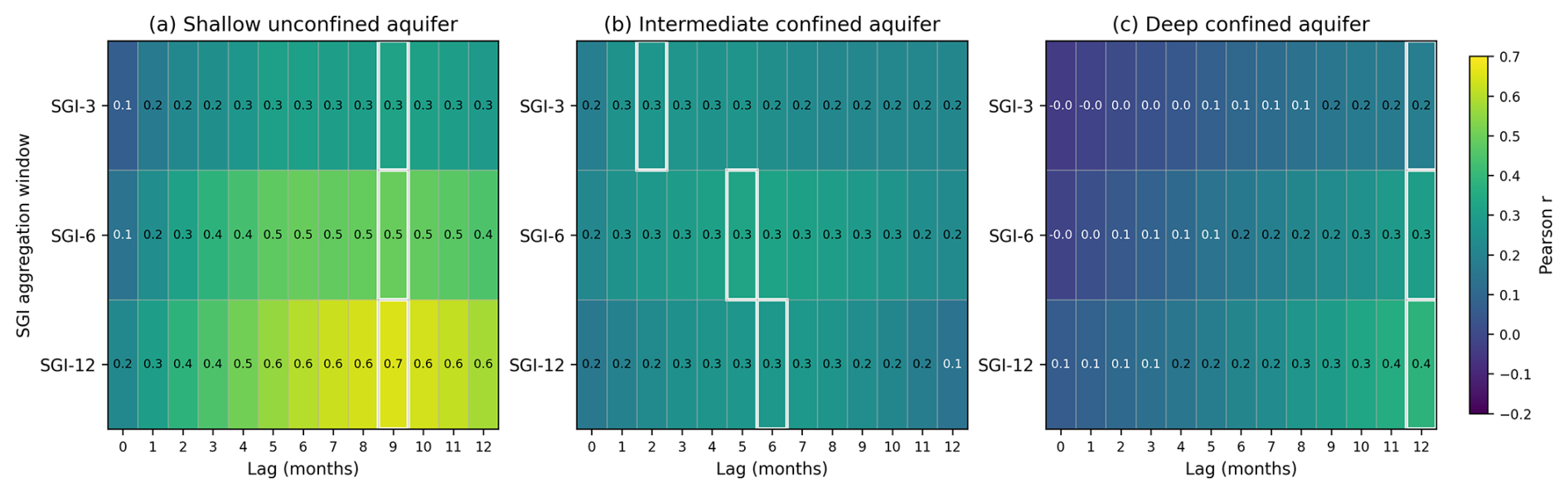
Figure B1 Full-period lagged SPI–SGI correlations for the three monitored aquifer systems in GWB 43. Panels show Pearson correlation coefficients between aquifer-group mean SGI and SPI from the meteorological station nearest to the corresponding aquifer-group centroid for (a) the shallow unconfined aquifer, (b) the intermediate confined aquifer, and (c) the deep confined aquifer. Correlations were calculated separately for the 3-, 6-, and 12-month aggregation scales over lags of 0–12 months. White outlines mark the lag associated with the maximum correlation in each row. Positive lags indicate that SGI follows SPI. Maxima occurring at 12 months represent the upper boundary of the tested range and do not exclude longer response delays.

Appendix C

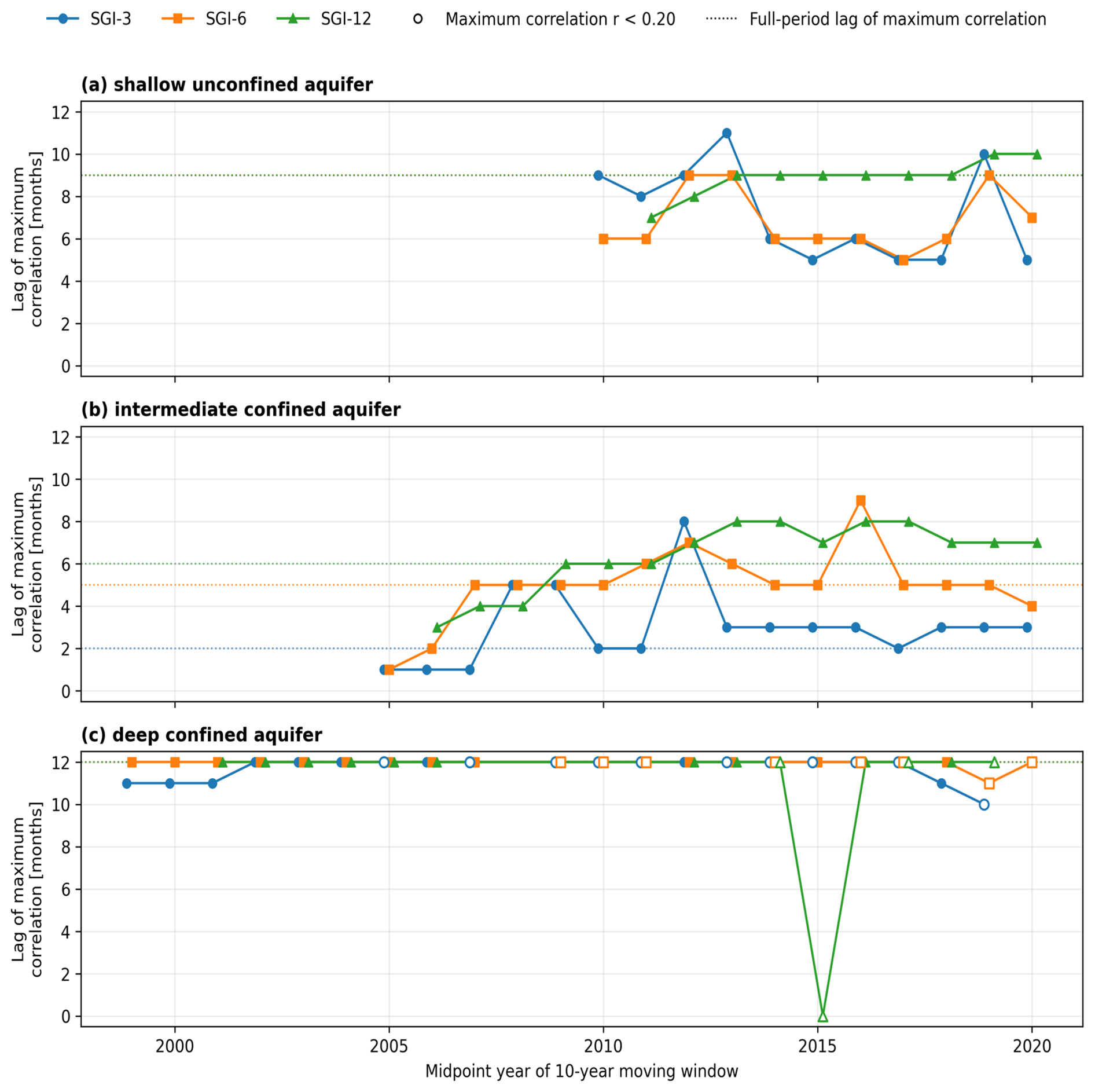
Figure C1 Temporal stability of the lag associated with the maximum SPI–SGI correlation in the three aquifer systems. The panels show results for (a) the shallow unconfined aquifer, (b) the intermediate confined aquifer, and (c) the deep confined aquifer, calculated using 10-year moving windows shifted forward by 1 year. Symbols indicate the lag of the maximum Pearson correlation for SGI-3, SGI-6, and SGI-12. Open symbols denote cases in which the maximum correlation was weak (r<0.20). Horizontal dotted lines indicate the full-period lag of maximum correlation for each SGI aggregation scale. Values reaching the upper tested limit of 12 months indicate that the actual response delay may exceed the analysed lag range.

Appendix D

Table D1 LOOCV-based diagnostic of monitoring-network influence on interpolation uncertainty. Full-network RMSE values refer to the original leave-one-out cross-validation of the three normalised Exposure subcomponents. The exclusion scenarios represent diagnostic recalculation of error statistics from the existing LOOCV results after omitting the indicated held-out observations; interpolation surfaces were not regenerated. SSE share denotes the proportion of total squared LOOCV error attributable to the two indicated monitoring locations. Local metric contrast was defined as the absolute difference in the observed metric value between each piezometer and its nearest neighbouring monitoring point.