
the Creative Commons Attribution 4.0 License.
the Creative Commons Attribution 4.0 License.
 | 08 Sep 2026
Towards a global actual evapotranspiration product for the Copernicus Land Monitoring Service

Héctor Nieto
José Miguel Barrios
Walid Ghariani
Francoise Gellens-Meulenberghs
Jan De Pue
Roselyne Lacaze
Copernicus Land Monitoring Service (CLMS) produces biogeophysical maps of the global land surface. The CLMS portfolio so far did not include actual evapotranspiration (ETa), despite it being a direct link between the energy, water and carbon cycles and its importance for global food security, efficient water resources management and weather forecasting. However, a global CLMS ETa product was recently developed and entered operational production at the end of 2025. It consists of water flux (ETa, evaporation and transpiration) and energy flux (latent and sensible heat) sub-products, has a spatial resolution of 300 m, dekadal (10 d mean) temporal resolution for water fluxes and daily temporal resolution for instantaneous energy fluxes, is produced in near-real-time, and (like all other CLMS products) is distributed under free and open data policy. It is based mainly on Copernicus input data with primary satellite imagery coming from the observations of OLCI and SLSTR sensors on board of Sentinel-3 satellites. Such product fills a gap in previously existing global and operational ETa products, thus satisfying a wide range of potential users' needs. In this paper, we describe, evaluate and justify the various design choices taken during the development of the ETa product, ranging from cloud masking and gap-filling, through derivation of biophysical traits, radiation components and weather forcings to spatial sharpening of the land surface temperature observations. Those data were then used to drive two ETa models: TSEB-PT and ETLook. A prototype implementation of the ETa processing chain was used to produce ETa data (using both models individually and their ensemble) across a globally representative range of climatic zones and plant functional types, which was validated against measurements from 206 Eddy Covariance flux tower sites. The ensemble resulted in the all-site root mean squared error (RMSE) of 0.87 mm d−1 (relative RMSE of 47 %, site range: 0.31–1.96 mm d−1), bias of 0.01 mm d−1 (relative bias of 0.6 %, site range: −1.39–1.50 mm d−1) and correlation coefficient of 0.81 (site mean of 0.77), which compares well with WaPOR global ETa dataset and therefore supports the operational production of global, near-real time, Copernicus-based 300 m ETa maps. Finally, we propose a number of potential evolutions of the CLMS ETa product, including enlarging and enhancing the model ensemble, producing a reanalysis version of the product with more robust meteorological forcing and improved gap-filling, and focusing on aspects of modelling related to influence of surface roughness and soil moisture on energy and water fluxes.
- Article
(20978 KB) - Full-text XML
- BibTeX
- EndNote


Copernicus (https://www.copernicus.eu, last access: 1 September 2025) is the Earth observation (EO) program of the European Union that provides free and open access to data acquired by the Sentinel satellites (and other contributing missions) and to higher level and non-space products through the Copernicus services. One of the main objectives of the program is to bring operational mindset to EO by: (1) providing data in near-real-time (NRT) with regular updates and derived using robust and validated methods; (2) guaranteeing long-term future continuity of this data and predictable planning of future evolutions. The Copernicus Land Monitoring Service (CLMS – https://land.copernicus.eu, last access: 1 September 2025) produces a series of qualified global biogeophysical products on the status and evolution of the land surface. The products are used to monitor vegetation, water cycle, energy budget and terrestrial cryosphere. Production and delivery are carried out in a timely manner and are complemented by the constitution of long-term time series.
Actual evapotranspiration (ETa) can be defined as the phase change from liquid to gaseous water that is transferred from the land surface towards the atmosphere. It can be partitioned between evaporation and transpiration through plants, with the former component implicitly including also evaporation from intercepted water in the canopy. It has historically not been included in the CLMS portfolio. This changed at the end of 2025 when the CLMS near-real-time (NRT) ETa product entered operational production (https://land.copernicus.eu/en/products/evapotranspiration, last access: 28 January 2026). This product will be of importance for many applications and research questions. The ETa is one of the Essential Climate Variables (ECV) as defined by the Global Climate Observing System (Bojinski et al., 2014). It binds different processes occurring at the Earth's surface (related to energy, water and carbon cycles) and evolves coherently with other biophysical variables, including those which are part of the CLMS portfolio (e.g. leaf area index, gross primary productivity, soil moisture, surface temperature). Since actual evapotranspiration is a direct proxy of plant water use it can be utilized for consistent agricultural water use monitoring across natural and political boundaries, and is therefore essential for Sustainable Development Goal (SDG) reporting, e.g. of SDG indicators 6.4.1 and 6.4.2 (O'Connor et al., 2020). ETa can also be useful for forest fire risk/spread forecasting (Vidal et al., 1994), drought monitoring (Anderson et al., 2011), hydrological modelling (Zhang et al., 2020; Larsen et al., 2016), irrigation accounting (Zhang and Long, 2021) and yield modelling (Jurečka et al., 2021; Gómez-Candón et al., 2021). In addition, spatially distributed fields of ET at an adequate spatial resolution can help to improve weather forecasting (Boone et al., 2025), in particular in irrigated fields in semi-arid climates where the additional water supply in the soil affects the surrounding microclimate and thus the atmospheric boundary layer conditions (Udina et al., 2024; Lunel et al., 2024).
One of the initial primary users of the CLMS ETa product is the Food and Agriculture Organisation (FAO) of the United Nations. FAO has been producing and disseminating ETa datasets, including a global product, through its “WAter Productivity through Open-access of Remotely sensed derived data” (WaPOR – https://www.fao.org/in-action/remote-sensing-for-water-productivity/en, last access: 30 July 2025) project. The WaPOR data has been used in multiple applications such as improving water use productivity or monitoring agricultural practices and water consumption (Chukalla et al., 2022; Hajirad et al., 2023; Seijger et al., 2023). Since there is no guarantee of long-term continuity of the WaPOR project, FAO expressed strong interest to the European Commission for the introduction of a global ETa dataset in the CLMS portfolio (https://www.fao.org/in-action/remote-sensing-for-water-productivity/news-and-events/news/news-detail/copernicus-global-land-service-launches-new-global-evapotranspiration-product-based-on-the-wapor-etlook-model/en, last access: 1 May 2026).
Table 1Specifications (requirements) of the Copernicus Land Monitoring Service actual evapotranspiration product based on call for tenders JRC/2023/OP/0273 (https://ec.europa.eu/info/funding-tenders/opportunities/portal/screen/opportunities/tender-details/13795, last access: 11 August 2026).
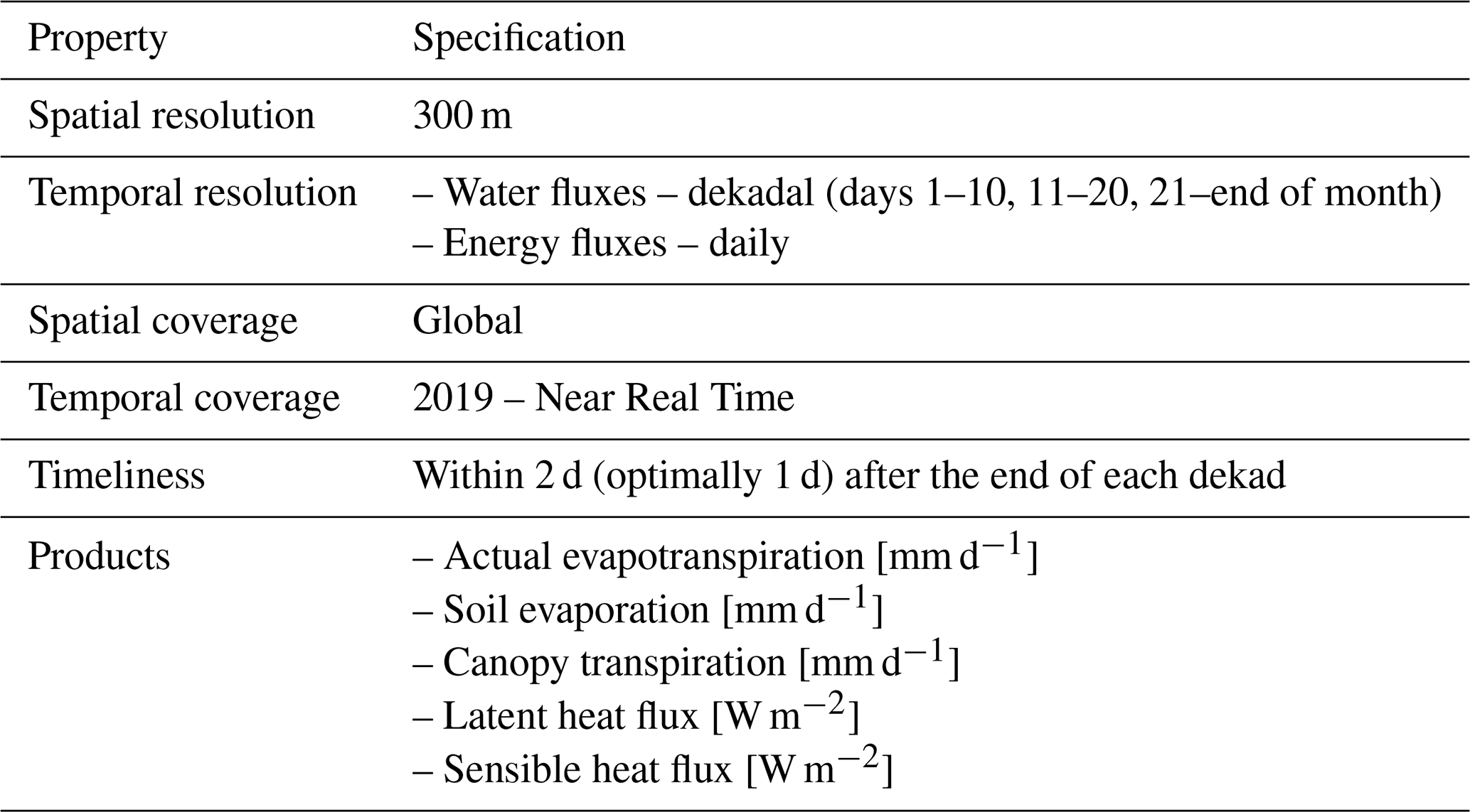
Developing a global, operational product is constrained by certain programmatic, financial and technical limitations. The CLMS products are designed for long-term continuity and are funded by the European Commission. Therefore, issues like compute efficiency, data storage and dissemination costs or long-term availability of sources of core input data need to be considered. Taking those constraints into account, and in order to satisfy a wide range of potential users needs while ensuring consistency with vegetation, primary productivity and other global CLMS products, the European Commission set the requirements for the CLMS ETa product of 300 m spatial resolution, dekadal temporal resolution for water fluxes sub-products and data availability in NRT (within 2 d after the end of each dekad). The product requirements are summarized in Table 1. Those requirements in turn impact the design choices presented in this study for the first version of the CLMS ETa product.
Those requirements also closely match the specifications of the WaPOR global ETa dataset and fill a gap in currently available satellite-based ETa products. Apart from WaPOR (the long-term continuity of which is not guaranteed), global operational ETa datasets produced in NRT with closest matching spatio-temporal specifications are the MODIS and VIIRS ETa products (Román et al., 2024). They have a higher temporal resolution (8 d) but lower spatial resolution (500 m) and use a modeling approach which does not make direct use of land surface temperature (LST) measurements (Mu et al., 2011). Another operational and global product which utilizes MODIS and VIIRS data is produced by United States Geological Survey for their Famine Early Warning Systems Network (FEWS NET) using SSEBop energy balance model (Senay et al., 2020) with dekadal temporal resolution and 1 km spatial resolution. Other ETa datasets have either much lower spatial resolutions (e.g. ETa product based on geostationary observations produced by the EUMETSAT Satellite Application Facility on Land Surface Analysis – Barrios et al., 2024, or the microwave-based GLEAM model – Miralles et al., 2011), do not have global coverage (e.g. OpenET – Melton et al., 2022) or are not produced in NRT (e.g. ETMonitor – Zheng et al., 2022).
Preparatory activities required to develop an operational CLMS ETa product recommended that ET models from two modelling frameworks should be further investigated. The first one is the Sen-ET framework (Guzinski et al., 2020, 2021) developed to model ETa with Copernicus data at various spatial scales and using the Two-Source Energy Balance Priestley-Taylor (TSEB-PT) ET model (Norman et al., 1995; Kustas and Norman, 1999; Anderson et al., 2024). The second is the WaPOR framework developed by FAO through the WaPOR project and using the WaPOR ETLook ETa model (hereafter referred to as ETLook) closely based on Bastiaanssen et al. (2012). Both models, although conceptually different, estimate evaporation and transpiration and use LST as one of core input forcings. This recommendation was mainly based on the availability of mature open-source implementations of the two ET models, on previous studies demonstrating the applicability of both models with Copernicus data sources (i.e. Sentinel-3 imagery and meteorological data from European Center for Medium Range Weather Forecasts) (Guzinski et al., 2021) and on FAO's familiarity with both approaches. This does not imply that those two modelling frameworks clearly outperform all other approaches and indeed it has been shown that the performance of an individual model depends on the landcover and climatic conditions (Reitz et al., 2025). However, due to constraints on developing a publicly funded global and operational dataset (outlined previously) there was a need to limit the design of the first version of the CLMS ETa product to those two frameworks.
This paper aims to describe, evaluate and justify the design choices made for the CLMS ETa product. In Sect. 2, we present the design of the CLMS ETa processing chain, starting with a brief outline of the two ETa models, followed by the description of input data sources and their pre-processing and finishing with the method used for gap-filling of the resulting maps. This is followed by Sect. 3 in which a prototype ETa dataset, produced with both TSEB-PT and ETLook and their ensemble, is validated against measurements from 206 Eddy Covariance (EC) flux tower sites. In Sect. 4, we compare the modelled outputs with each other and with other similar ET datasets, evaluate and justify the design choices described in Sect. 2 and outline suggestions for product improvement. Finally, conclusions are presented in Sect. 5.
2.1 ET modelling
2.1.1 TSEB-PT model
The Two-Source Energy Balance (TSEB) modelling scheme was proposed by Norman et al. (1995) and afterwards refined and applied in a multitude of applications and studies (Anderson et al., 2024) including the Sen-ET framework (Guzinski et al., 2020) and implemented as open source in pyTSEB Python package (Nieto et al., 2025a). In this modelling scheme the directional radiometric LST (TR(θ)) is split into the temperatures of vegetation (TC) and soil (TS) based on Leaf Area Index (LAI) and LST observation geometry.
where θ is the view zenith angle of the thermal observation and Ω(θ) is the clumping factor of the vegetation at view angle θ (Kustas and Norman, 1999) and has a value of less than 1 for clumped vegetation.
Based on this split, the energy fluxes of vegetation and soil (net radiation – Rn, sensible heat flux – H, latent heat flux – λE, soil heat flux – G) are estimated separately, before being combined to obtain the bulk surface fluxes.
The soil (canopy) sensible heat flux is computed from the gradient between the soil (canopy) temperature (TS and TC respectively) and the air temperature at the sink-source height. This transfer of heat between the two components and the atmosphere is modulated by resistances to heat exchange (ra,S (Kustas and Norman, 1999; Kondo and Ishida, 1997; Sauer and Norman, 1995) and ra,C (McNaughton and Van Den Hurk, 1995), respectively) organized in a series resistance network (in analogy to electrical systems) which depend on canopy structure (roughness) and weather (wind and atmospheric stability) conditions.
Since there are multiple solutions to TC and TS satisfying Eq. (1), an iterative approach is employed. The initial assumption is that green canopy transpires at potential rate based on Priestley-Taylor formulation (Priestley and Taylor, 1972):
where αPT is the Priestley-Taylor coefficient, fg is the fraction of vegetation that is green and thus transpiring, Δ is the slope of the vapour pressure to air temperature curve (hPa K−1) and γ is the psychrometric constant (hPa K−1). In all land-covers αPT has an initial value of 1.26, except for coniferous forests where it is lowered to account for reduction in stem conductivity (and therefore stomatal conductance) with height () and broadleaved and mixed forests where it is assigned a value of 0.82, both following Komatsu (2005). If unrealistic fluxes are obtained (λES<0 indicating condensation in the soil during daytime) during this first iteration, then the canopy transpiration (i.e., αPT) is sequentially reduced and soil and canopy temperatures and fluxes are recalculated until realistic values are obtained. This implementation of the TSEB scheme is called the TSEB-PT model.
TSEB-PT outputs instantaneous fluxes at the time of thermal image acquisition. The modelled instantaneous latent heat flux (λEinst), calculated during clear-sky conditions, can be extrapolated to daily ET values as (Cammalleri et al., 2014), where and are the daily and instantaneous shortwave irradiances, respectively.
2.1.2 ETLook model
ETLook model (Bastiaanssen et al., 2012) is used in the WaPOR framework and is described in detail in the Methodology section of the WaPOR ETLook wiki (https://github.com/un-fao/wapor-et-look/wiki/Actual%20Evapotranspiration%20and%20Interception#methodology, last access: 22 January 2026) (FRAME Consortium, 2024). Similarly to TSEB-PT, ETLook is a two-source model, meaning that it derives soil evaporation (E) and vegetation transpiration (T) as two separate fluxes, and it ensures conservation of energy at the land-surface. The model assumes potential rates of daily E and T based on the Penman–Monteith equation (Monteith, 1965) that are throttled down to actual E and T using stress factors:
where Δe (hPa) is vapor pressure deficit, ρ (kg m−3) is the air density, cp (J kg−1 K−1) is specific heat of dry air, ra,S and ra,C are aerodynamic resistances for heat turbulent transport for soil and canopy respectively calculated following Allen (1998) and adjusted for buoyancy using Monin-Obukhov similarity theory in unstable conditions, and rS and rC are resistances of water transfer in respectively the soil and canopy. All resistances are in s m−1.
The resistance of soil to water vapour transfer is calculated as
where rs,min is minimum soil resistance with constant value of 800 (s m−1), c is a power factor with a constant value of −2.1 and is relative top-soil soil moisture (Camillo and Gurney, 1986).
The canopy stomatal resistance is affected by air temperature stress (St), vapour pressure stress (Sv), radiation stress (Sr) and root-zone soil moisture stress (Sm)
where rst,min (s m−1) is the minimum stomatal resistance and LAIeff is effective leaf area index (Jarvis, 1976; Stewart, 1988).
In addition, ETLook estimates evaporation from rainfall intercepted by the canopy (I in mm d−1):
where P is precipitation, and FVC is fractional vegetation cover. The energy used in this process is subtracted from net radiation (Rn) before it is split into the soil and canopy components (Rn,S and Rn,C respectively) and used to estimate E and T in Eq. (7).
The main difference between WaPOR implementation of ETLook and Bastiaanssen et al. (2012) is the method of obtaining soil moisture required for E and T stress factors. In Bastiaanssen et al. (2012) it is based on microwave observations while in WaPOR ETLook it is derived using a trapezoid constructed in the LST – vegetation fractional cover (fC) space (Yang et al., 2015). The trapezoid corner values are set based on theoretical calculations by inverting the Penman-Monteith equation for both dry and moist bare soil and vegetated conditions. Then the soil moisture of a pixel (representing both top-soil and root-zone) is estimated using the relative location of LST and fC of that pixel within that trapezoid. The CLMS implementation of ETLook adopts the WaPOR methodology. The one major difference between the WaPOR and CLMS ETLook-derived fluxes is that the former includes I as a separate sub-product while the latter does not. To ensure consistency of ETLook model formulations, we pass rainfall estimates to the ETLook and let it calculate I internally, before adding it to E calculated in Eq. (7):
This aligns also with TSEB-PT model in which I is implicitly included in evaporation. EETLook,CLMS is referred to as evaporation from ETLook in the rest of this manuscript.
Apart from land-cover dependent parameters (see Sect. 2.2.6), ETLook uses other spatially-distributed but temporally constant parameters (e.g. theoretical albedo of bare soil and full vegetation cover used during soil moisture estimation) which are provided as maps distributed by FAO.
2.2 Input data sources
Modelling actual evapotranspiration with satellite observations and TSEB-PT or ETLook models is a complex task requiring diverse set of input forcing variables (Table 2). Those are derived from shortwave optical imagery needed to estimate biophysical properties of the surface (e.g. leaf area index – LAI and albedo), thermal infrared observations of land surface temperature which is the boundary condition for the land surface – air energy exchange and a proxy for root-zone soil moisture, weather forcing, which drive (e.g. solar irradiance) and modulate (e.g wind speed) the energy exchange between the land surface and the air, and ancillary data (e.g. digital elevation models and canopy height maps) that cannot be derived from the other data sources.
Table 2Input forcing variables for Copernicus Land Monitoring Service actual evapotranspiration product. PAR indicates photosynthetically active radiation part of the spectrum (400–700 nm) while NIR indicates near infra-red part of the spectrum (700–2500 nm).
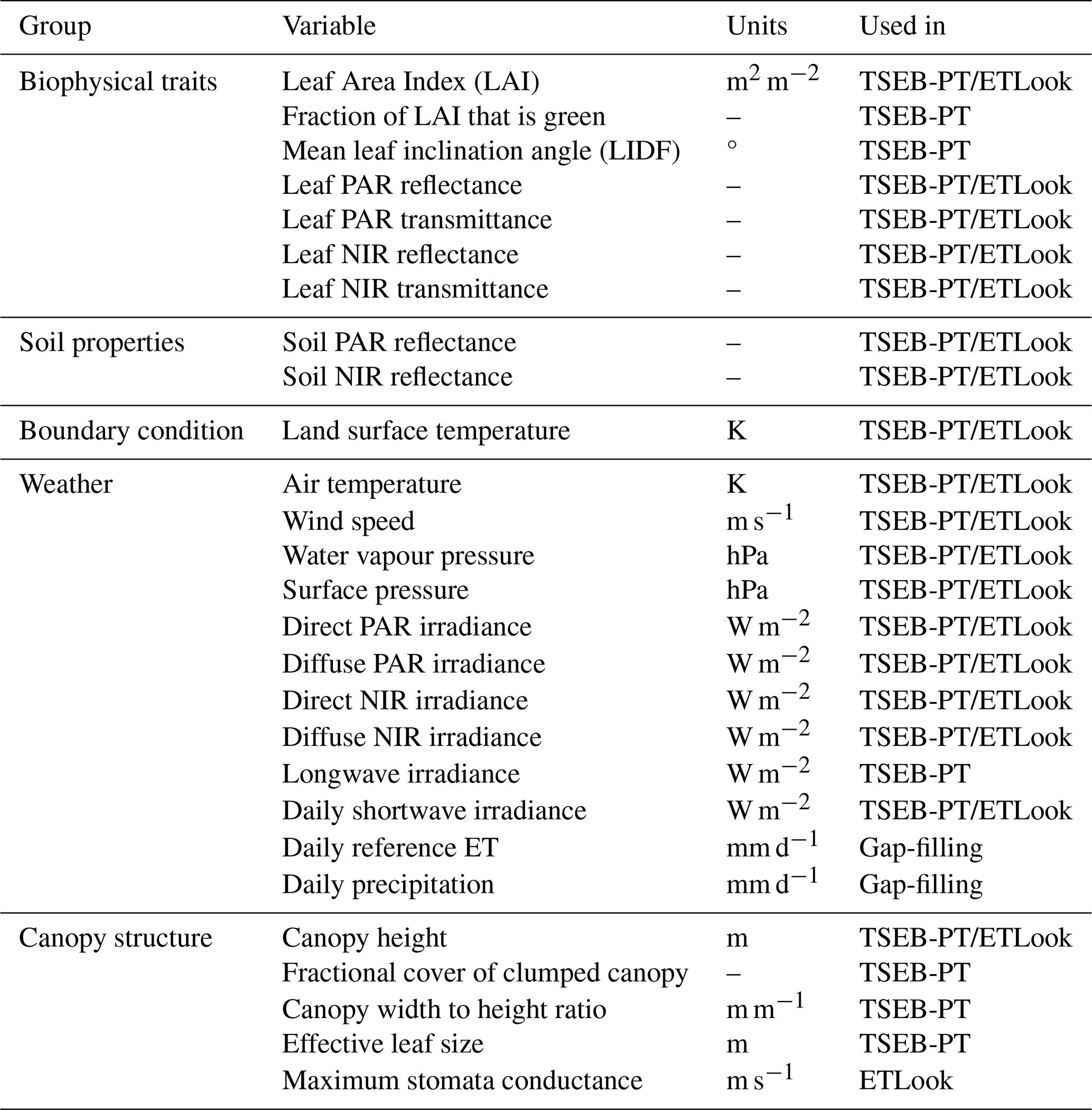
Copernicus products should, to the largest extent possible, be based on other Copernicus data. This is to ensure the free and open license conditions, long-term future continuity and consistency across the CLMS portfolio. In case of the CLMS ETa product, this means observations from optical (both shortwave and thermal infrared) sensors on board of Sentinel-3 satellites and Copernicus Digital Elevation Model (DEM – European Space Agency and Airbus, 2022), both available from the Copernicus Data Space Ecosystem (https://dataspace.copernicus.eu/, last access: 25 August 2025), and products provided by CLMS and Copernicus Atmosphere Monitoring Service (Peuch et al., 2022) (Table 3). The only exception is the canopy height map, which is derived from fusion of GEDI LiDAR measurements and Sentinel-2 imagery (Lang et al., 2023).
Table 3Input data sources for the Copernicus Land Monitoring Service actual evapotranspiration near-real-time product.

The subsections below describe the pre-processing methods selected to convert the input data from Table 3 into ET model input forcing variables shown in Table 2.
2.2.1 Sentinel-3 cloud-masking and gap-filling
Biophysical characterization of the land-surface is based on imagery obtained by two sensors on-board Sentinel-3 satellites: shortwave Ocean and Land Colour Intrument (OLCI); and combined shortwave and thermal infrared Sea and Land Surface Temperature Radiometer (SLSTR). Both sensors operate in the optical spectral domain, which is blocked by clouds and therefore cloud detection and masking needs to be performed before further analysis of these data.
Atmospherically corrected and geolocated Top-Of-Canopy (TOC) reflectances derived from shortwave optical detectors on OLCI and SLSTR sensors are generated and distributed by the CLMS (Copernicus Land Monitoring Service, 2025b). The cloud mask of this product is based on quality flags from Level 1 SLSTR and OLCI products and IDEPIX approach (Wevers et al., 2022). No further cloud masking is performed during the ETa production and instead the recommendations on using the annotation flags from Sect. 5.1 of Product User Manual (Copernicus Land Monitoring Service, 2025d) are followed.
Land Surface Temperature (LST) product (SL_2_LST___) is a Level 2 product based on thermal observations by the SLSTR sensor. It comes with quality layers indicating the presence of clouds. As recommended in the Copernicus Sentinel-3 SLSTR Land User Handbook (https://sentiwiki.copernicus.eu/__attachments/a_0b084365 0153c5e0933699cf9259d22d5995022524c99c86c744555f7 ebe3af4/OMPC.ACR.HBK.002%20-%20Sentinel%203%20 SLSTR%20Land%20Handbook%202024%20-%201.4.pdf? cb=e7c5d241da616f170b23f3a61f552a4e, last access: 27 August 2026), the probabilistic cloud mask is used during ETa production. This cloud mask uses a semi-Bayesian approach by estimating a probability of a clear-sky using radiative transfer modelling and meteorological conditions at the time of satellite overpass and observational climatology (Bulgin et al., 2014).
The TOC reflectance is used to derive land surface biophysical traits (Sect. 2.2.2) and albedo (Sect. 2.2.3) and to sharpen the LST (Sect. 2.2.4). The reflectance values, as well as biophysical traits, usually show a clear seasonal cycle and spatial similarity, and have same or similar values in both cloudy and sunny conditions (e.g. leaf area index does not change day to day depending on cloudiness). Therefore, gaps in this data are highly suitable for filling using spatio-temporal gap-filling, e.g. StarFM (Gao et al., 2006), and smoothing methods, e.g. Whittaker-Eilers smoother used by WaPOR (Eilers, 2003). On the other hand, LST is highly variable in both time (the temperature can change significantly at short time intervals even though it also has a strong seasonal cycle) and space. In addition, LST under clouds is different to LST in clear-sky conditions (Abbasi et al., 2020). This makes gap-filling of LST particularly difficult and using inaccurately gap-filled values can lead to energy imbalance at the land surface. Therefore, LST is usually not gap-filled, especially if it is to be used as input into ETa models.
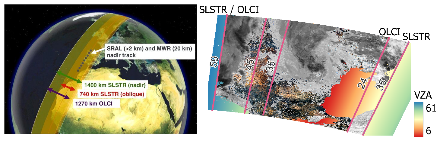
Figure 1Widths and locations of swaths of Sentinel-3 OLCI and SLSTR instruments (courtesy of Donlon et al., 2012) (left) and maximum view zenith angles (VZA) of those swaths overlaid on an example OLCI (colour) and SLSTR (greyscale) image (right). Also indicated are potential limits of VZA on the western side of the swath (45 and 35°).
In the case of the CLMS ETa product, we are using TOC reflectance and LST observations acquired by sensors onboard the same satellite platform and thus observing the land surface (and the clouds) at the same time. Therefore, since LST is not gap-filled, there is also no need to gap-fill TOC reflectance acquired at the same time and location. However, the Sentinel-3 OLCI sensor has a swath width of 1270 km, while the nadir pointing scan of SLSTR sensor has a swath width of 1400 km (Donlon et al., 2012). Both sensors are tilted to reduce the sun glint effect and therefore larger part of the swath is located westwards of the satellite orbit path (Fig. 1, left).
The sensors are positioned such that their swaths align at the western edge, while on the eastern edge the coverage of OLCI ends at view zenith angle (VZA) of 24° while coverage of SLSTR ends at VZA of 35° (Fig. 1, right). When modelling ETa, LST observations acquired at high VZA (e.g. above 45° as in the Sen-ET approach; Guzinski et al., 2020) are usually omitted due to increased uncertainty caused by longer atmospheric path, LST anisotropy and larger pixel footprint. However, SLSTR observations from the eastern edge of the swath with VZA between 24 and 35° could still potentially be used if OLCI data for that part of the swath was gap-filled.
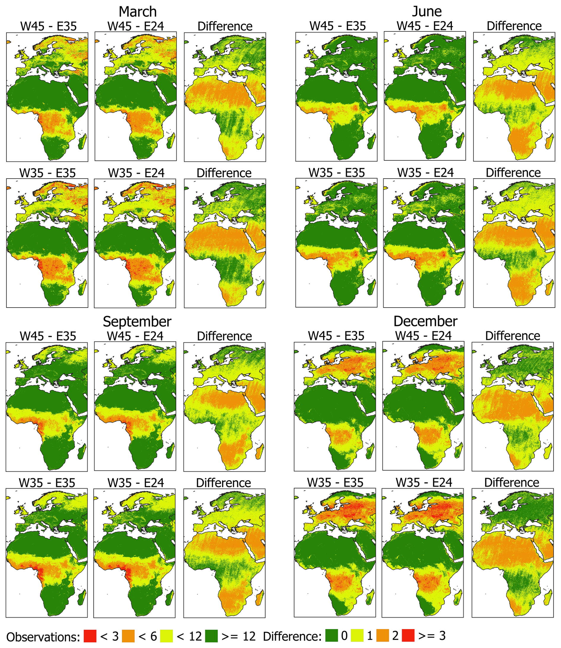
Figure 2Mean number of monthly cloud-free SLSTR observations for period 2020–2024 (apart from March 2020 and December 2024) for March (top-left), June (top-right), September (bottom-left) and December (bottom-right). The titles of the sub-plots indicate view zenith angle (VZA) limits on the western and eastern edges of the swath (e.g. W45–E35 indicates a VZA limit of 45° on the western edge and 35° on the eastern edge). The last column of each panel shows the difference in cloud-free observations per month between limiting eastern swath to either 35° or 24°. Less than 3 observations per month means on average less than one observation per 10 d aggregation period (dekad), less than 6 per month means less than 2 per dekad, less than 12 per month means less than 4 per dekad.
To assess whether it is worth to gap-fill the missing part of OLCI's eastern swath, and whether maximum VZA should be limited to 45° or 35° (threshold mission requirement value for planned Copernicus Land Surface Temperature Monitoring mission; Koetz et al., 2021), we performed an analysis of number of monthly cloud-free Sentinel-3 LST acquisitions over Europe and Africa (Fig. 2). This analysis was performed using 5 years of data (2020–2024) for months of March, June, September and December (apart from March 2020 and December 2024) and while limiting VZA of the western edge of swath to either 45° or 35° and eastern edge to either 35° or 24°.
Figure 2 shows a clear seasonal trend in the number of cloud-free SLSTR observations. In June and September, most of Europe has sufficient number of cloud-free observations for each dekad (at least 2 but often more than 4), while in March and, especially in December, there are areas where less than two or even less than one cloud free observations are available in each dekad. In the equatorial region of Africa, there are predominantly cloudy conditions throughout the year but they shift north in June and September and south in December and March. The difference between number of monthly cloud-free observations with eastern VZA limited to 35° or 24° is in large majority of cases less than 2, except in the Sahara region and southern Africa where there is sufficient number of observations in either case. The difference between limiting western swath to either 45° or 35° is more pronounced and can push some regions to having less than 1 observation per dekad.
Based on this analysis, it was decided to limit the western VZA to 45° and eastern VZA to 24°. This means that the extra processing that would be required to gap-fill the OLCI swath is avoided. Even though gap-filling of input imagery will not be performed, the filling of cloud gaps in the produced ETa maps is required to fulfill the requirements of the ETa product. Therefore gap-filling of outputs will be performed as described in Sect. 2.3.
2.2.2 Biophysical traits
A sound and generalizable approach to obtain the biophysical traits required by the ETa models is the inversion of canopy radiative transfer models (RTM), such as the combined PROSPECT (Jacquemoud and Baret, 1990; Feret et al., 2008; Féret et al., 2017, 2021) and 4SAIL (Verhoef et al., 2007) RTMs. Together those models can simulate the canopy spectra from 400 to 2500 nm at every nm based on the inputs listed in Table 4 (Jacquemoud et al., 2009). One computationally efficient inversion method consists of training a regression model based on large number of PROSPECT and 4SAIL simulations (Weiss et al., 2000, 2002; Verrelst et al., 2012). Then this regression model is applied to the spectral imagery to obtain the biophysical traits maps.
Campbell (1990)Table 4List of biophysical traits and ancillary information required by PROSPECT-D+4SAIL radiative transfer models together with range of values which are simulated or set during the simulation. Ranges are based on information extracted from the LOPEX database (Hosgood et al., 1993) and the Sentinel-2 Biophysical ATBD (Weiss et al., 2020).
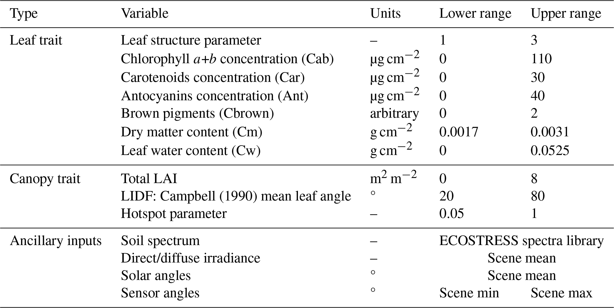
In case of CLMS ETa, we are using a vectorized version of Féret et al. (2017) PROSPECT-D and Verhoef et al. (2007) 4SAIL models (Nieto, 2025). This vectorized version allows us to run the RTMs very efficiently and thus enables us to generate specific regression models for each scene, given their actual observation and illumination conditions. This contrasts with other similar algorithms, such as the BiophysicalOp in the Sentinel-2 toolbox of Sentinel Application Platform (Djamai et al., 2019), which applies the same generic hybrid inversion approach to all scenes. The biophysical processing framework is summarized as:
-
Estimating the proportion of spectral direct and diffuse irradiance using the 6S model (Vermote et al., 1997) and mean sun zenith and azimuth angles together with mean aerosol optical thickness and total column water vapor of Sentinel-3 TOC scene.
-
Generating ca. 40 000 PROSPECT-D+4SAIL simulated spectra by:
- a.
Creating the same amount of Monte Carlo random samples (Saltelli et al., 1999) of biophysical traits and observation angles, based on prescribed plausible ranges listed in Table 4.
- b.
Running PROSPECT-D+4SAIL for each of these samples together with the generated proportion of spectral direct and diffuse irradiance and the mean solar angles of the scene.
- c.
Convolving the simulated narrowband spectra using the Sentinel-3 OLCI and SLSTR spectral response functions in order to obtain a set of 40 000 simulated Sentinel-3 TOC reflectances.
- a.
-
Training a random forest regression in which the dependent variables are the randomly generated biophysical traits and the explicative variables the correspondent simulated TOC reflectances and observation angles.
-
Applying the random forest regression to the actual TOC reflectance scene.
As outputs we obtain 8 products: leaf area index (LAI), Campbell (1990) mean leaf angle, leaf chlorophyll a+b concentration, leaf carotenoids concentration, leaf antocyanin concentration, brown pigments, leaf dry matter content, and leaf water content. The retrieved leaf pigments concentration gives us an idea about the canopy greenness, and we have observed an increase of Sentinel-3 estimated antocyanin concentration during vegetation curing in summer and the leaf senescence in fall. Indeed antocyanins are red pigments and thus may become dominant over other leaf pigments in those situations (Féret et al., 2017). For that reason, we can express the fraction of LAI that is green (fg) using an empirical piecewise linear relation to the antocyanins (Ant):
2.2.3 Albedo and net shortwave radiation
Net radiation (Rn) provides the energy that drives all other energy fluxes at the land-surface (including ET) and can be approximated as:
where Sn (S↓) and Ln (L↓) are the shortwave and longwave net radiation (incoming irradiances) respectively, α and ϵ are surface albedo and emissivity, respectively, LST is the Land Surface Temperature, and (W m−2 K−4) is the Stefan-Boltzmann constant.
Considering the larger magnitude of shortwave irradiance (S↓) compared to the longwave irradiance (L↓), and the fact that Ln is usually computed internally by each ET model, we will focus on method for deriving Sn. In particular, this study concentrates on the canopy and leaf properties that influence albedo and radiation partitioning between soil and canopy. The albedo (α) is defined as the proportion of incident shortwave radiation that is reflected by the surface. The shortwave net radiation (Sn) is therefore the balance between the incident shortwave irradiance (S↓) and the reflected shortwave radiance ().
The spectral properties of the surface are key in determining the albedo. Leaves, due to their photosynthetic activity, absorb a large proportion of light due to the presence of chlorophylls, as well as other leaf pigments. On the other hand, soils can have a large range of albedo values, depending on their mineral composition, texture and topsoil moisture. Therefore, the albedo of a vegetated surface, and also radiation partitioning between soil and canopy, will depend not only on leaf chlorophyll concentration but also on canopy density and, in a lesser degree, on the soil albedo in situations of sparse vegetation or initial growth stages. Indeed, most of the Earth's surface show certain anisotropic behaviour when reflecting radiation i.e. it scatters different amounts of radiation depending on the scattering direction. Vegetation, as it is mainly composed by an array of leaves, is also affected by this anisotropic behaviour. Therefore, plants will reflect radiation differently depending on their structural characteristics as well as the illumination geometry (i.e. the solar position) and the scattering direction (i.e. the sensor position), changing their albedo with time.
To compute the net shortwave radiation and its partitioning between the canopy (SnC) and the soil (SnS) the model of Campbell and Norman (1998) is used. The key aspect of this model is the calculation of the transmitted shortwave radiation through the canopy (τC), which is wavelength dependent due to vegetation absorbing a greater portion of photosynthetically active radiation (PAR – 400–700 nm) than near infra-red (NIR – 700–2500 nm) wavelengths. τC is partitioned into two components (direct/diffuse) and in two spectral band (PAR/NIR).
where ρC,DIR is the canopy directional-hemispherical reflectance, ρC,DIF is the canopy bihemispherical reflectance, τC,DIR canopy directional-hemispherical transmittance, τC,DIF canopy bihemispherical transmittance, which depend on leaf spectral properties (absortance) and canopy structure (LAI and leaf inclination distribution parameter; Campbell, 1990). On the other hand, ρS is the soil bihemispherical reflectance. In all cases τ and ρ are separated between the PAR and NIR regions of the solar spectrum. The calculation of canopy transmittances and reflectances is shown in Appendix A.
Campbell RTM requires the leaf absorptance () as input for calculating canopy transmittance and reflectance. To estimate this parameter, we are using the leaf traits retrievals from the biophysical processor described in Sect. 2.2.2. With the information of these traits, we can run the PROSPECT-D leaf RTM in forward mode to get a spectral reflectance (ρ) and transmittance (τ) that could then be integrated to the required broadband regions. However, running PROSPECT-D for a large array of pixels is too computationally expensive. For that reason, a PROSPECT-D emulator (Guzinski et al., 2021) was developed (Rivera et al., 2015): we generated broadband leaf reflectances and transmittances in the PAR and NIR from a large range of PROSPECT-D simulations, covering all plausible range of leaf traits from Table 4, which was then used to train a random forest model that relates the leaf traits to the broadband PAR and NIR leaf reflectance and transmittance. Figure 3 depicts the importance that each leaf trait has on the broadband reflectance emulator, showing that the most important pigment is the chlorophyll a+b concentration, due to its strong absorption of PAR radiation, followed by the leaf dry matter and water contents, which are the main absorbers of the NIR/SWIR radiation.
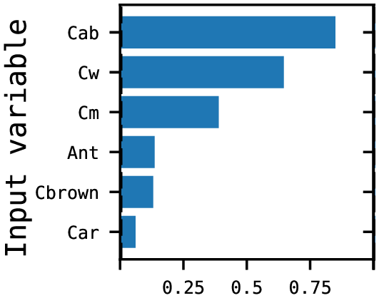
Figure 3Mean permutation importance for leaf biochemical components in the PROSPECT-D leaf radiative transfer emulator. Cab – chlorophyll a+b concentration, Cw – leaf water content, Cm – dry matter content, Ant – antocyanins concentration, Cbrown – brown pigments concentration, Car – carotenoids concentration.
Soil reflectance has a smaller role in most situations, since the radiation reaching the ground is smaller due to the interception of light by the canopy. However, in sparse and semi-arid conditions, where vegetation is scarce or even not present, soil albedo plays a significant role. Furthermore, these semi-arid areas are usually characterized by brighter soils since they are composed by sands, salts and with a small fraction of organic matter. For that reason, Guzinski et al. (2023) developed a method to unmix the broadband soil reflectance (ρsoil,λ) from the TOC reflectance:
where P0(θv) is the canopy gap fraction at the satellite observation angle θv computed by the Beer-Lambert law (), ρsurface,λ is the broadband surface reflectance, and ρleaf,λ is the leaf broadband reflectance computed previously.
Table 5Narrowband to Broadaband conversion coefficients for Sentinel-3A and Sentinel-3B platforms.

In order to convert the narrowband reflectances of the TOC product into broadband reflectances we have applied the approach proposed by Liang (2001), who derived a linear regression model between the satellite spectral bands and the broad bands corresponding to the PAR region (400–700 nm), NIR region (700–2500 nm) and the solar spectrum (SW – 400–2500 nm). Similarly to Liang (2001), to overcome the limited amount of in situ measurements of albedo, we again made use of the PROSPECT-D+4SAIL canopy RTM coupled with the 6S atmospheric RTM (Vermote et al., 1997) to run a large number of simulations covering all plausible illumination, atmospheric and canopy conditions. Once the RTM simulations are performed (at 1 nm step), we convolved the results to both Sentinel-3A and Sentinel-3B specific spectral response functions, and integrated these simulated spectra to the broadband regions defined above. Then, one multivariate linear regression model per broadband region and per platform is fitted with the broadband reflectances as dependent variables and the Sentinel-3 simulated TOC reflectances as explanatory variables. The resulting coefficients are shown in Table 5, showing the weight of each Sentinel-3 band has on the broadband reflectances. It is worth noting that the coefficients are consistent with the expected behaviour, since the spectral bands located in the PAR region have no influence on the NIR broadband reflectances, nor the spectral bands in the NIR/SWIR influence on the PAR broadband model.
2.2.4 Land surface temperature sharpening
The CLMS ETa product specification states a spatial resolution of 300 m. However, the spatial resolution of the SLSTR LST product is 1 km. Therefore, a method to perform thermal sharpening of the LST is required. Most such methods are based on machine learning approaches, of various complexities, which capture the relationships between shortwave spectral reflectance (and possibly other ancillary data) and the LST. The shortwave reflectance is of higher spatial resolution and is resampled to the resolution of LST to be used as explanatory variables for model training. Once trained, the model is applied to the reflectance at its original resolution to obtain a representation of LST at that resolution. In most approaches, this is followed by a bias correction step to ensure conservation of energy between the LST maps at both the original and sharpened spatial resolutions (Agam et al., 2007; Gao et al., 2012; Sánchez et al., 2020).
Both the Sen-ET and WaPOR (version 3) modelling frameworks use a Data Mining Sharpener (DMS) thermal sharpening approach (Gao et al., 2012) as implemented in the pyDMS Python package (https://github.com/radosuav/pyDMS, last access: 30 July 2025). It is a quite complex method that however works well even for sharpening by a ratio of 50 i.e. sharpening Sentinel-3 LST from 1 km to 20 m using Sentinel-2 reflectance (Guzinski and Nieto, 2019; Guzinski et al., 2023; Sánchez et al., 2024). Based on this work, we are applying it to sharpen Sentinel-3 LST using CLMS TOC product with 300 m spatial resolution. The DMS regression models are trained on the whole Sentinel-3 TOC tile (10° by 10°) as well as on subsets of 30 by 30 LST pixels in a moving window fashion.
In Sen-ET framework all relevant reflectance bands from Sentinel-2 or Sentinel-3 (depending on the target spatial resolution) covering visible, near-infrared and shortwave-infrared parts of the spectrum were used as explanatory variables. For Sentinel-3 this means the following 17 bands from CLMS TOC product: Oa02, Oa03, Oa04, Oa05, Oa06, Oa07, Oa08, Oa09, Oa10, Oa11, Oa12, Oa16, Oa17, Oa18, Oa21, S5N, S6N. This configuration of variables, in addition to DEM and cosine of solar inclination angle, is called “DMS – Reflectance” in Sect. 4.3.2. During the WaPOR project, feature engineering was performed and spectral bands were converted to indices before evaluating their usefulness in DMS (FRAME Consortium, 2024). This resulted in following 11 spectral bands, reflectance indices and DEM-related products being used as explanatory variables: Oa04 (blue), Oa17 (NIR), Modified Normalized Difference Water Index (MNDWI), Plant Senescence Reflectance Index (PSRI), Normalized Difference Moisture Index (NMDI), Visible Atmospherically Resistant Index Red Edge (VARI_RED_EDGE), Bare Soil Index (BI), elevation, cosine solar inclination angle, aspect and slope. More details and the list of evaluated indices are available in the WaPOR wiki (https://github.com/un-fao/wapor-et-look/wiki/Land%20Surface%20Temperature#processing-approach, last access: 22 January 2026). This combination of explanatory variables is called “DMS – WaPOR” in Sect. 4.3.2. Finally, since the main influence of aspect and slope on LST is already captured in the solar inclination angle variable and their additional impact on sharpened LST accuracy is negligible (see Sect. 4.3.2), those two variables were removed from the WaPOR list. The resulting combination of 9 variables (called “DMS – WaPOR selected” in Sect. 4.3.2) is used in the ETa processing chain to sharpen the 1 km Sentinel-3 LST to the required 300 m spatial resolution.
2.2.5 Weather forcing
Weather forcing is critical for accurate estimation of ET. Due to the 2 d timeliness requirements for the CLMS ETa product, the weather data source is Copernicus Atmosphere Monitoring Service (CAMS) forecasts (Peuch et al., 2022), produced by the European Center for Medium Range Weather Forecasts and distributed freely and openly through the CAMS Data Store. CAMS data contain surface meteorological parameters with forecast runs every 12 h covering the whole Earth on a 0.4° grid and hourly temporal resolution. In this study we used CAMS forecasts with 12 h lead time also for the production of historical data to ensure fair comparison with the NRT dataset.
Table 6List of required CAMS global atmospheric composition forecast fields and their topographic correction status.
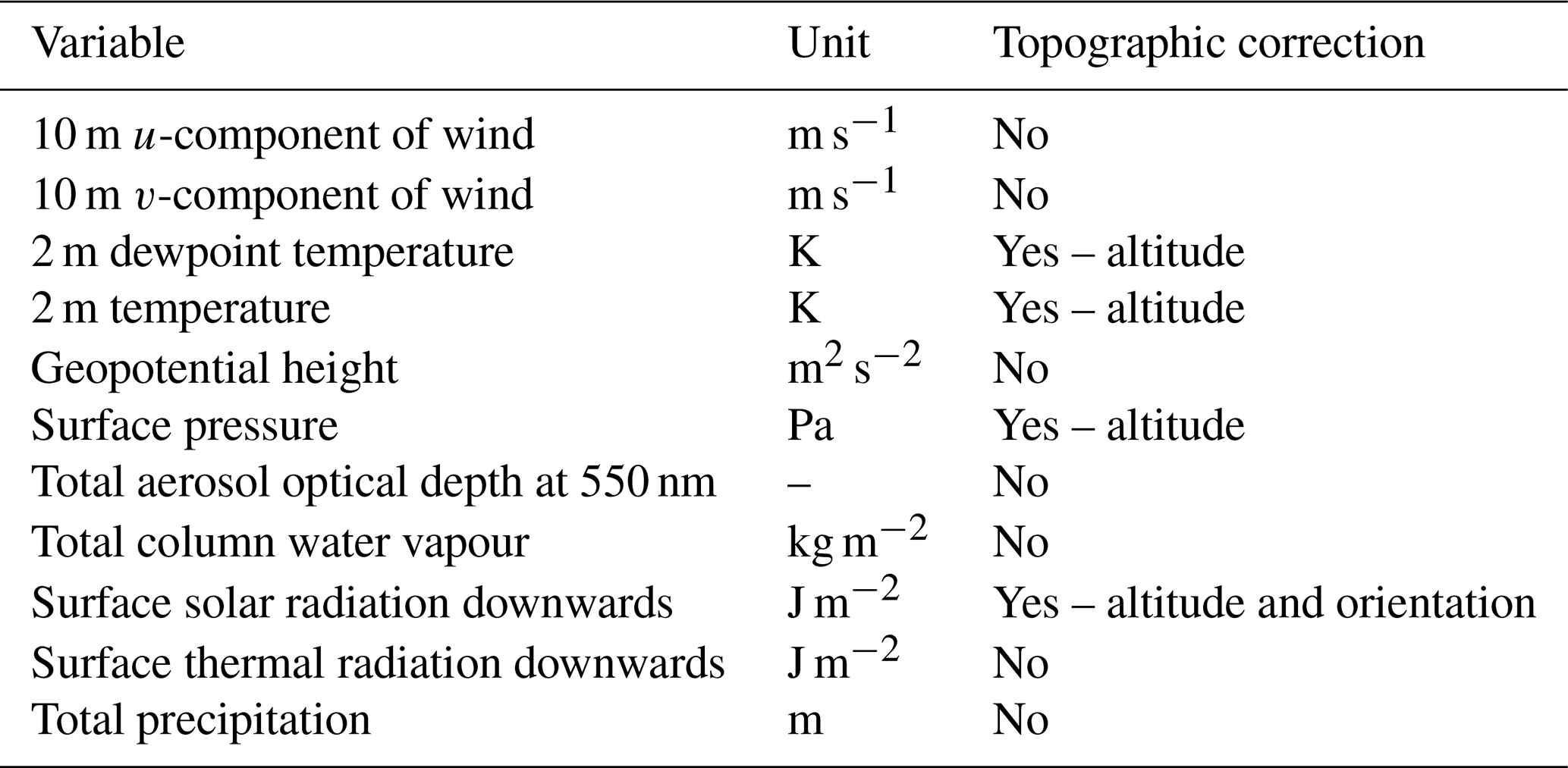
Instantaneous weather forcing at the satellite overpass are used to drive both ET models and include air temperature, vapor pressure, wind speed, surface pressure, and clear-sky solar irradiance (Table 6). All instantaneous data were obtained by linear interpolation between two CAMS hourly forecasts to the time of Sentinel-3 SLSTR acquisition over the area of interest. Daily weather forcing is used to drive the ETLook ET model and to extrapolate and interpolate the instantaneous estimates of ET and include solar irradiance as well as air and dew temperatures, wind speed, and pressure, which are then used to calculate the FAO-56 reference ET (Allen, 1998) required for the gap filling (see Sect. 2.3). They are being integrated over a 24 h period starting at midnight local time.
The pre-processing of CAMS weather forcing, including topographic correction, was done using the open source Python software meteo_utils (Nieto et al., 2025b) and as described in Guzinski et al. (2021). The only differences from Guzinski et al. (2021) being the use of Copernicus DEM (COP-DEM_GLO-90-DTED – European Space Agency and Airbus, 2022) resampled to a resolution of 300 m for topographic correction and the use of REST2 model (Gueymard, 2008) to estimate instantaneous clear sky solar irradiance and its PAR and NIR, beam and diffuse components. In addition daily total precipitation is calculated using 24 h integration of CAMS hourly total precipitation forecasts.
2.2.6 Structural and ancillary parameters
Resistance energy balance models need additional ancillary inputs, such as canopy height or roughness. The latter influences the efficiency of the turbulent transport of heat and water between the land surface and the overlying air (Raupach, 1994; Alfieri et al., 2019). Vegetation structure and density are thus important for estimating turbulent transport of momentum, heat and water vapour in the canopy air space (Garratt and Hicks, 1973; Thom, 1972; Raupach, 1994; Shaw and Pereira, 1982).
Table 7Land Cover (LC) Look-Up-Table for ancillary and structural parameters required by ET models, adapted from Guzinski et al. (2020). hmin (m) is the minimum canopy height; hmax (m) is the maximum canopy height occurring when leaf area index (LAI) reaches its optimal maximum LAImax (for annual plant functional types only); fc is the at-nadir fraction of the ground occupied by a clumped canopy (fc=1 for a homogeneous canopy); is the canopy shape parameter, representing the canopy width to canopy height ratio; lw (m) is the average leaf size; and rst (s m−1) is the minimum stomatal resistance. LC classes come from the CLMS Dynamic Land Cover map. Note that snow/ice and water surfaces are masked in the current implementation.
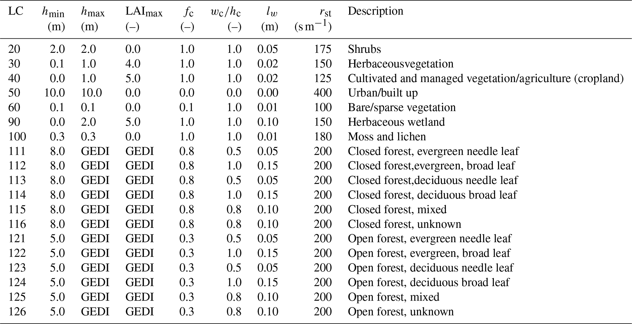
For that reason, the CLMS Global Dynamic Land Cover map (Copernicus Land Monitoring Service, 2015) is used to assign vegetation parameters, which are difficult to estimate directly from other Earth Observation data (Guzinski et al., 2021). Those parameters, and values assigned to different plant functional types, are listed in Table 7. The TSEB-PT model requires all of the parameters, apart from stomatal resistance, while ETLook requires only vegetation height and stomatal resistance. Values of all parameters, except for vegetation height of forested land covers, were adapted from Guzinski et al. (2020).
Vegetation height is one of the most important of the ancillary parameters, especially for the TSEB model (Burchard-Levine et al., 2020), as it influences the aerodynamic resistance to heat transport. In order to better estimate the obstacle (canopy) height in different land covers we use a framework that differs depending on predominant plant functional type of each land cover. For annual plant functional types, canopy height is dynamically computed considering its growth as:
where the symbols are described in Table 7.
For forest plant functional types we set a static canopy height based on a 10 m spatial resolution (averaged to 300 m resolution) global forest canopy height map developed by combining the Global Ecosystem Dynamics Investigation (GEDI) LiDAR and Sentinel-2 observations using a probabilistic deep learning model (Lang et al., 2023). Whenever the land cover map indicated a forest while the GEDI-based canopy height map was below the hmin parameter, the minimum value was enforced.
2.3 Output gap-filling and temporal compositing
The CLMS ETa product consists of 5 sub-products: instantaneous sensible and latent heat fluxes (in W m−2), and dekadal (10 d mean) evapotranspiration and its components evaporation and transpiration (in mm d−1). The instantaneous heat fluxes represent values modeled at the time of Sentinel-3 satellite overpass and, therefore, do not undergo any gap-filling. On the other hand, the daily water fluxes (used for the production of the dekadal sub-products) need to undergo gap-filling. Otherwise, the dekadal mean would only take into account fluxes modeled during clear-sky conditions within the aggregation period. This would firstly result in frequent gaps and secondly in a systematic overestimation of the dekadal aggregate. The data availability is strongly time and region dependent, but the majority of the dekades have fewer than 6 daily ET estimates per pixel. To illustrate this, Fig. 4 shows the number of valid observations in the first dekad of July 2021 across the globe.
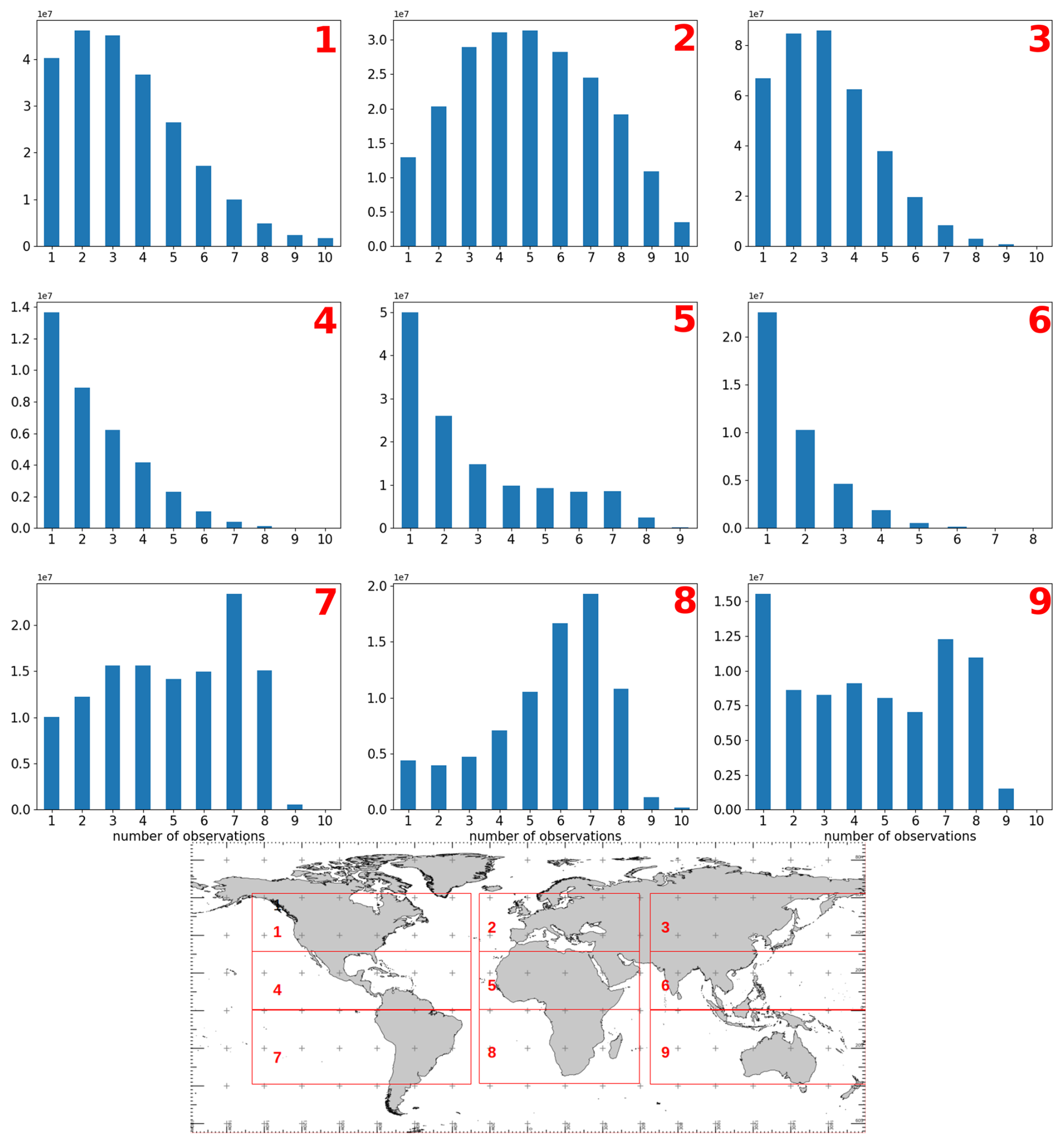
Figure 4Number of land pixels (y-axis) having 1–10 observations on the first dekad of July 2021 per region of the world.
The gap-filling of ET product, i.e. estimation of ET during cloudy conditions, is usually performed using a reference quantity that can be derived for any date regardless of cloud conditions. This implies that this reference quantity is mostly dependent on weather forcing. In the Sen-ET approach the choice was made to use reference evapotranspiration calculated using the FAO-56 method (Allen, 1998). A ratio of modeled daily ETa to reference ET (called crop-stress coefficient Ks,c) is calculated on dates for which daily ETa is available and is used to recreate ETa on the target date which needs to be gap-filled, as described in Guzinski et al. (2021). This method was further developed in Guzinski et al. (2023) to better account for soil drying by performing linear interpolation of Ks,c (applicable only in non-NRT modelling when ETa after the target date is available) and for soil wetting through rainfall by setting Ks,c to the maximum value observed during the gap-filling period if a simple water-balance approach indicates sufficient moisture in the soil. Taking rainfall into account is important especially for longer gap-filling periods (Delogu et al., 2021) and in climates in which rainfall initiates the growing season (e.g. rainy season in the Sahel and other semi-arid areas). For the CLMS ETa processing chain we further improved the robustness of this method, especially for longer gap-filling windows, by replacing the maximum Ks,c observed within the gap-filling window with the 80th percentile of ratios observed within the gap-filling period. If the latest know Ks,c before the target date was larger than 80th percentile then the value of that last know Ks,c was preserved. This was done to ensure that taking rainfall into account would only increase, and not reduce, the gap-filled ET values. To accommodate longer periods with few satellite observations (see Fig. 2) a 60 d gap-filling window is used during ETa production.
Once the gap-filled ET is estimated, the split into evaporation and transpiration is performed using the ratio of evaporation or transpiration to ET from the closest non-gap-filled preceding date. The all-sky gap-filled daily estimates of evapotranspiration, evaporation and transpiration are then aggregated to dekadal timesteps by taking the mean of all valid values within the aggregation period. Finally the Ensemble dataset is computed by averaging the gap-filled evapotranspiration, evaporation and transpiration estimates from the TSEB-PT and ETLook models. The degree of gap-filling for a given dekad is indicated in the quality layers as the number of valid modelled clear-sky (i.e. not gap-filled) ET values within each dekad and the average temporal distance (in days) between the gap-filled ETs within a given dekad and the closest previous valid clear-sky modelled ET.
The main aim of the validation is to evaluate the performance of the prototype product through comparison of dekadal ETa values, as modelled by the TSEB-PT and ETLook algorithms, with ETa data derived from in-situ measurements in the period 2020–2022, from stations covering main worldwide climatic zones and plant functional types. In addition to assessing the performance of the two ETa models driven by input forcing as described in Sect. 2, the statistical metrics were also computed for an ETa dataset composed by the average of the TSEB-PT and ETLook estimates. This additional dataset is referred to as Ensemble ETa (Volk et al., 2024). The statistical metrics used in the analysis were: bias, root mean squared error (RMSE) and Pearson correlation coefficient (r). This comparison focused only on the variables that could be extracted from measurements at eddy covariance stations (ETa, λE, H). Evaporation and transpiration were generated by the models but could not be routinely contrasted against in situ observations and therefore accuracy of partition of ET into E and T is uncertain.
3.1 Validation data collection and preparation
The search for eddy covariance sites was intended to collect data representing the largest possible diversity of climate regions and plant functional types. Different eddy covariance networks and datasets were explored in search for validation data for recent years. The years 2020–2022 were selected for this analysis considering the overall in situ data availability.
When building the reference database we used the energy balance closure (EBC) (Foken et al., 2011) correction provided by the dataset, in order to ensure transparency and minimize scientific bias. Therefore, priority was given to datasets in which λE and H data had been corrected for EBC problem. A commonly applied procedure delivering corrected values of λE and H is the ONEflux processing which uses the Bowen Ratio correction method (Pastorello et al., 2020). Data generated by this procedure could be obtained from the AmeriFlux (FLUXNET dataset) (Novick et al., 2018), ICOS (Integrated Carbon Observations System – Heiskanen et al., 2022) and OzFlux (Isaac, 2014) networks. In search for more diversity in the reference datasets, other networks/datasets were queried even if the processing chain was not accounting for the EBC. Thus, data from the European Fluxes Database Cluster (EFDC – https://www.europe-fluxdata.eu/, last access: 1 September 2025), l'observatoire AMMA-CATCH (Analyse Multidisciplinaire de la Mousson Africaine – Couplage de l'Atmosphère Tropicale et du Cycle Hydrologique – Galle et al., 2018; AMMA-CATCH, 1990), AsiaFlux (Mizoguchi et al., 2009), JapanFlux (Ueyama et al., 2025), South African Environmental Observation Network (SAEON, https://observationsmonitor.saeon.ac.za, last access: 15 January 2026) and AmeriFlux (BASE dataset) (Chu et al., 2023) networks were also included in the analysis.
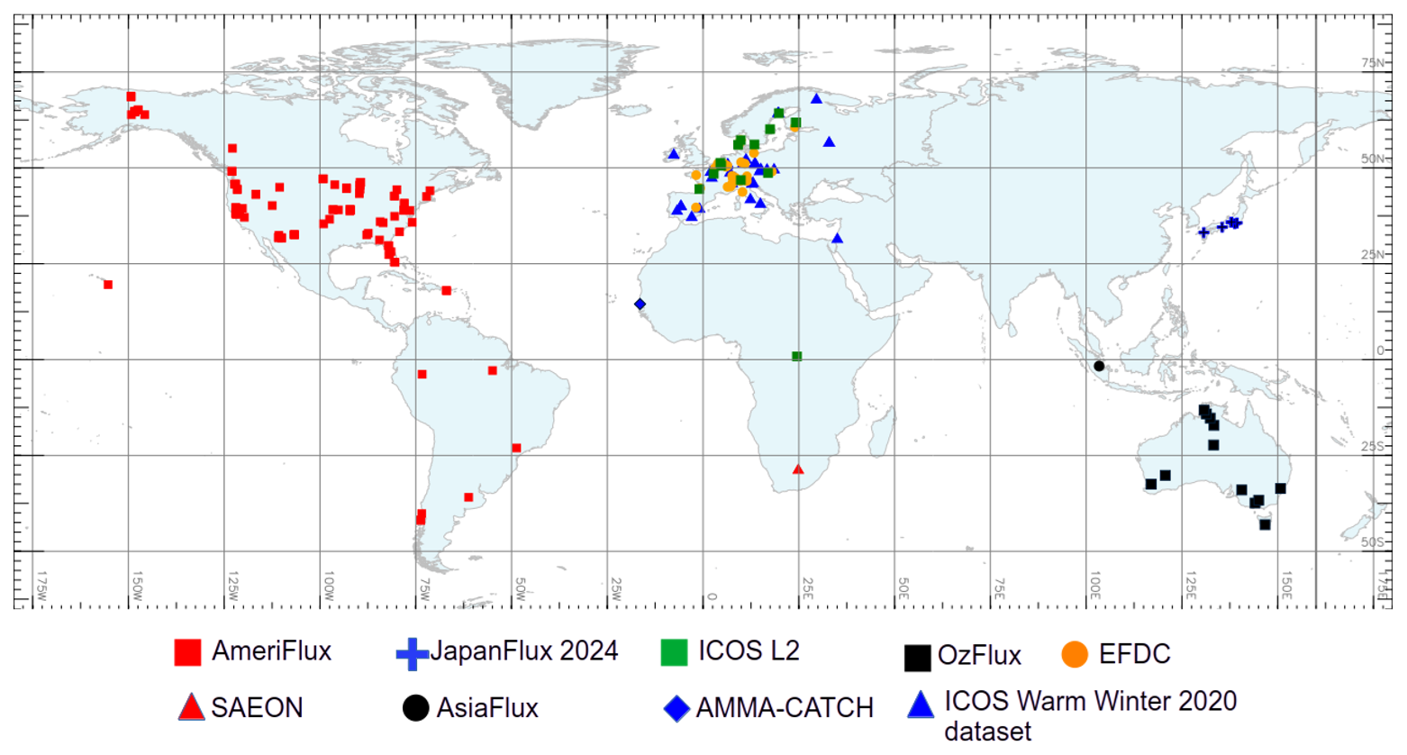
Figure 5Eddy covariance sites and networks used for ETa validation.
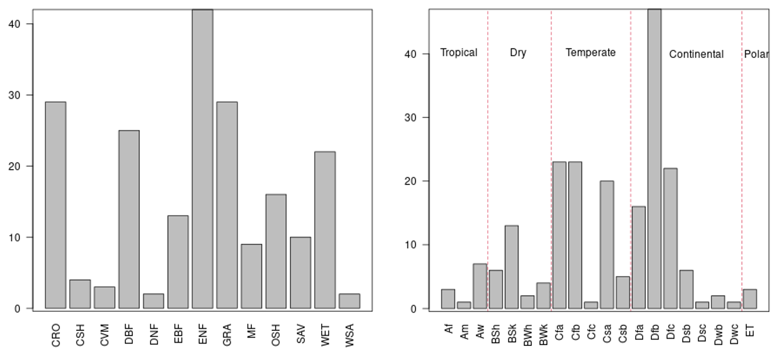
Figure 6Number of eddy covariance sites grouped per PFT (left) and per Köppen climate region (right). CRO: Cropland; CSH: Closed Shrubland; CVM: Crop Vegetation Mosaic; DBF: Deciduous Broadleaved Forest; EBF: Evergreen Broadleaved Forest; ENF: Evergreen Needleleaved Forest; GRA: Grassland; OSH: Open Shrubland; SAV: Savanna; URB: Urban; WET: Wetland; WSA: Woody Savanna.
Figure 5 shows the location of the eddy covariance sites considered in this study and the network/dataset the data were taken from, while Fig. 6 provides an overview of the representation of climate regions and plant functional types (PFT) in this set of eddy covariance sites. Further details of the location, climate, PFT and network of each site can be found in Appendix B.
Figures 5 and 6 show that the available eddy covariance networks are not equally distributed across the globe which results in imbalanced representativeness of climate regions and plant functional types. However, there are stations located in all major climate zones and PFTs and across all continents (except Antarctica). Despite lack on in-situ measurements in some larger geographical areas (mainly in Asia, Africa and South America), there are other sites which are located in similar climatic zones, e.g. tropics (northern Australia) as well as arid and semi-arid (Spain, southern Australia and western US). Therefore, we believe that the validation should be representative also of the geographical areas for which in-situ ET data is currently missing.
The data acquired from the AmeriFlux, ICOS and OzFlux networks was available at half-hourly and daily time steps and format aspects like variable naming, units, quality flags, etc. were uniform. Daily λE data were discarded if the value of the quality flag was lower than 0.6 (i.e. less than 60 % of sub-daily data was measured or had a good quality gap filling). A dekadal ETa value was computed if the dekad was composed of at least 7 valid daily ETa values. The computation of ETa from λE and air temperature was conducted as follows:
where lv is the latent heat of vaporization, Ta is the average daily air temperature, λE is the daily average latent heat flux and ET is the daily evapotranspiration in mm d−1.
The data from other networks was delivered at half-hourly time step only. Therefore, an additional aggregation step needed to be considered to obtain daily ETa values. In doing this, the half-hourly data were filtered using quality flag (provided with the data) to remove invalid and poor quality values. For each day, the number of valid timeslots between sunrise and sunset was computed (the sunrise and sunset times change as function of geographic location and time of the year). Missing half-hourly data during the day were computed by linear interpolation if the number of valid timeslots during daytime was at least 50 % of the total number of timeslots in that period. Otherwise, the day was discarded. The criterion for aggregating the daily ETa values to dekadal values was the same as indicated in the previous paragraph.
The last preparatory step was matching the modelled and reference values on the basis of timeslot and location. The temporal matching is a straightforward step for the dekadal ETa values. The data at satellite overpass time (λE and H) were matched to the nearest timeslot of the eddy covariance half-hourly datasets. The satellite overpass time, in local time, varied along the year for the different sites. For instance, the AU-Cum site registered values between 09:05 and 10:52 local time (LT); US-Ton, between 10:03 and 11:52 LT; ES-LM1, between 11:27 and 13:13 LT; etc. The analysis for λE and H at satellite overpass time was conducted for TSEB-PT only as the ETLook algorithm does not generate those variables. Spatial matching was performed on the basis of selecting the 300 m pixel within which the flux tower is located. The spatial scale mismatch between the flux tower footprint and the pixel size could affect the reported accuracy of the products, especially at heterogeneous sites and during stable atmospheric conditions.
3.2 Validation results
The procedure described in the previous section resulted in a dataset of over 13 000 records (206 sites) of dekadal ETa values obtained from eddy covariance measurements. A first appraisal on the performance of the ETa models can be obtained from the statistical scores shown in Table 8. A graphical representation of the performance of the models under consideration is presented in the Taylor plot of Fig. 7. The overall statistics (i.e. not at site level) were generated from the full dataset of observed and modelled ETa pairs across all the validation sites.
Table 8Bias (modelled − measured: mm d−1), Root Mean Squared Error (RMSE: mm d−1), and Pearson correlation coefficient (r) scores for dekadal ETa per model (all sites combined), and summary statistics at site level. rBias and rRMSE are relative metrics (i.e., divided by mean measured ET). SD stands for standard deviation.

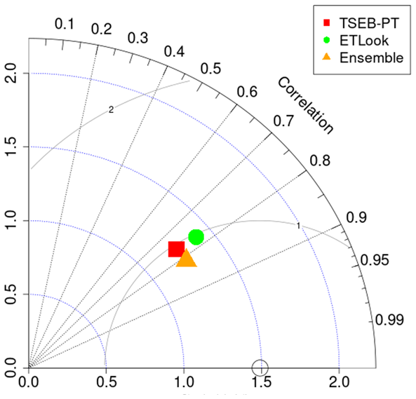
Figure 7Taylor-plot overview of ETa accuracies of TSEB-PT, ETLook and Ensemble dataset. Azimuthal angle represents the Pearson r, radial distance from the origin is the standard deviation (mm d−1). Circle marker at the horizontal axis represents perfect model performance, markers closer to this point indicate better model performance. Radial distance from this point is equivalent to centered RMSE (contour values shown in mm d−1). The statistics shown in the Taylor diagram were generated from the full dataset of observed and modelled ETa pairs across all the validation sites.
The points to be highlighted in these statistical scores are:
-
All ETa models exhibit high correlation with the in situ observations (r above 0.75).
-
Pairwise t-tests of the site-level validation results indicated that the Ensemble model had a significantly (p<0.05) higher r, lower RMSE and smaller bias, compared to TSEB-PT and ETLook.
-
The bias values of all three datasets are small (relative bias below 4 %) with Ensemble showing negligible bias.
Around 82 % of the data records used in calculating the scores of Table 8 and Fig. 7 had been corrected for the EBC problem. The same analysis was conducted for the subset of data records composed only of EBC-corrected data. The overall results were very similar to those presented above (Fig. C1 and Table C1), although not addressing the EBC issue could have large impact when looking at individual sites.
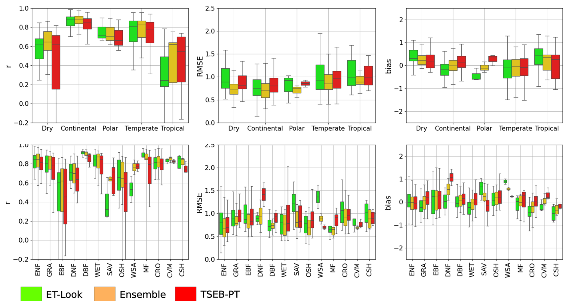
Figure 8Boxplots of r (left), RMSE (center) and bias (right) between in-situ observations and values of dekadal ET as computed by ETLook and TSEB-PT and the Ensemble dataset for years 2020–2022, for sites grouped per climates (top) or per plan functional types (bottom). The horizontal line indicates the median value, the box limits show the first and third quartiles, while the whiskers give the minimum and maximum value.
The plots of Fig. 8 show a more detailed view of these results, split into climate regions (based on Köppen climate classification system) and plant functional type classes. Complementary Taylor plots are available in Appendix C (Fig. C2 for climate regions and Fig. C3 for PFTs).
While ETLook and TSEB-PT have a different modelling approach, outputs of both models achieved comparable results in many cases. The CRO, GRA and WET and shrublands (CSH, OSH) Taylor plots reveal that both models exhibited similar performance in the generation of dekadal ETa values in those groups. The five classes together account for 49 % of the evaluated sites spread across different climate regimes and represent a wide range of conditions. The Ensemble ETa series exhibits slightly better correlation scores than the individual models.
Differentiating between climates, the r-score of the Ensemble was significantly better in continental and temperate climate regions, compared to dry and tropical regions (t-test p value < 0.05). In terms of bias, Ensemble ET estimates in dry climate regions had a significantly larger overestimation, compared to continental and temperate sites. This was also the case for tropical sites, though not significantly.
The sites in tropical and dry climates demonstrated the largest variability in model output performance and inter-model disagreement. This can also be observed in the classification according to PFT, where EBF, SAF, OSH and WSA exhibit a low and highly variable r. In tropical sites (and EBF sites), this is partly explained by the lack of pronounced seasonal cycle. In dry climates, this underlines the challenge to estimate ET under water-restricted conditions and the impact of different modelling approaches. Overall, the best scores were obtained with the Ensemble in tropical and dry areas, though a notable exception is the significantly smaller bias of TSEB-PT in the dry climate (0.17 mm d−1) compared to ETLook (0.31 mm d−1) and the ensemble (0.23 mm d−1). TSEB-PT also has the smallest bias in the tropics, though not significantly better than the other models.
Looking at PFTs, all models achieved the highest correlation in DBF (Ensemble median r: 0.92). However, this is not fully confirmed in the other validation metrics. Notably, the RMSE of TSEB-PT for this class is high (0.93 mm d−1), and significantly higher compared to ETLook and the Ensemble (0.72 and 0.74 mm d−1, respectively). Similar behavior was found in MF, where ETLook had a significantly lower RMSE, compared to TSEB-PT. This aligns with the underestimated variability of the fluxes (standard deviation in Fig. C3) in DBF and MF by TSEB-PT.
Conversely, ETLook had a significantly higher RMSE in SAV, compared to TSEB-PT. This corresponds to a large (positive) bias in ETLook for this class, whereas TSEB-PT has a small (negative) bias.
Some other classes also exhibit interesting behavior (e.g. contrasting RMSE and bias in DNF and WSA between models) but might be misleading due to small sample size (see Fig. 6) and are therefore not discussed here.
Table 9Bias (modelled − measured: W m−2), Root Mean Squared Error (RMSE: W m−2), and Pearson correlation coefficient (r) scores for instantaneous TSEB-PT λE and H (all sites combined), and summary statistics at site level. rBias and rRMSE are relative metrics (i.e., divided by mean measured λE or H).

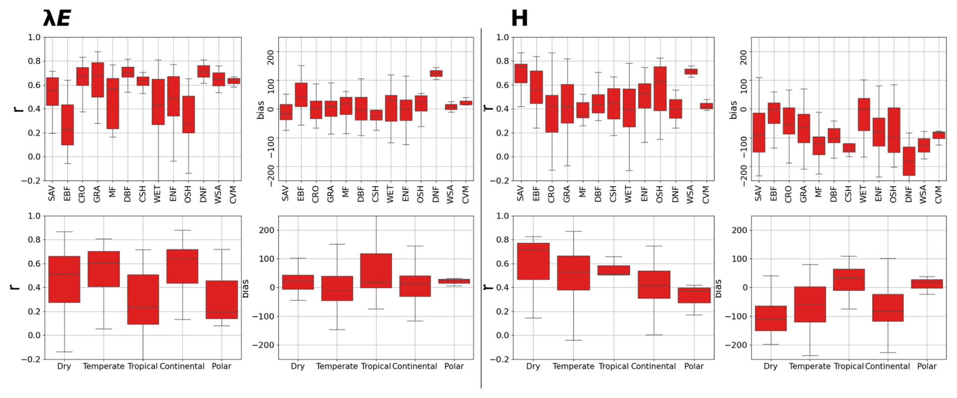
Figure 9Boxplots of r (left panels) and bias (right panels) values of λE (top panels) and H (bottom panels) at overpass time as modelled by the TSEB-PT model. The horizontal line indicates the median value, the box limits show the first and third quartiles, while the whiskers give the minimum and maximum value.
Table 9 shows the overall accuracy statistics and summary scores at site levels for λE and H, while Fig. 9 shows the range of r and bias values obtained for each climate and PFT class. A number of aspects in this plot can be connected to the analysis of dekadal ETa presented above. For instance, the large positive bias and low correlation of λE in the evergreen broadleaved forest (EBF) classes that is translated to the dekadal ET performance of Fig. 8. However, looking at the performance of H in EBF we see that TSEB-PT is explaining fairly well the variability in H, with mean correlation values of 0.6 and bias near 0 W m−2. An opposite behavior occurs for ENF, with a systematic underestimation of H but no bias in λE. It is also notable that the median bias in λE was positive and small (below 50 W m−2) in the majority of the sites while H estimates show a dominant negative bias with a larger magnitude, as can also be seen in timeseries modelled at the individual sites (Fig. C4). The length of the boxes in the boxplots of Fig. 9 suggests an important degree of variability in the correlation and error of the modelled values among the sites of each PFT class. Apart from modelling uncertainty, the differences in the time window at which satellite overpass takes place, the uncertainty associated with the in situ energy balance closure correction, and the large heterogeneity in ecosystem properties (e.g. heat storage) within each class can partly explain this variability and the differences between biases seen in H and λE.
Validation was not performed in urban areas since neither of the models is designed to estimate fluxes in those conditions. Urban areas present specific challenges when applying energy balance models due to, among other things, strong shadowing effects of buildings surrounding vegetated patches, increased complexity in modelling turbulent transport between surface and atmospheric boundary layer caused by the interaction between buildings of different heights and vegetated surfaces, and additional heat and water vapour sources interacting between themselves and with the atmosphere: buildings, paved roads, parks with different canopies coexisting (grass/trees). Therefore, a specific modelling approach for urban areas would be required to accurately account for those processes.
4.1 Comparison between the TSEB-PT, ETLook and Ensemble datasets
The validation assessment presented in Sect. 3 was based on the comparison of TSEB-PT, ETLook and Ensemble ETa estimates with measurements at eddy covariance towers and presented as one set of statistics for the whole validation period. However, the view of the spatial and temporal patterns in the ETa calculation by the ETLook and TSEB-PT models can give interesting insights towards the design of an operational ETa product.
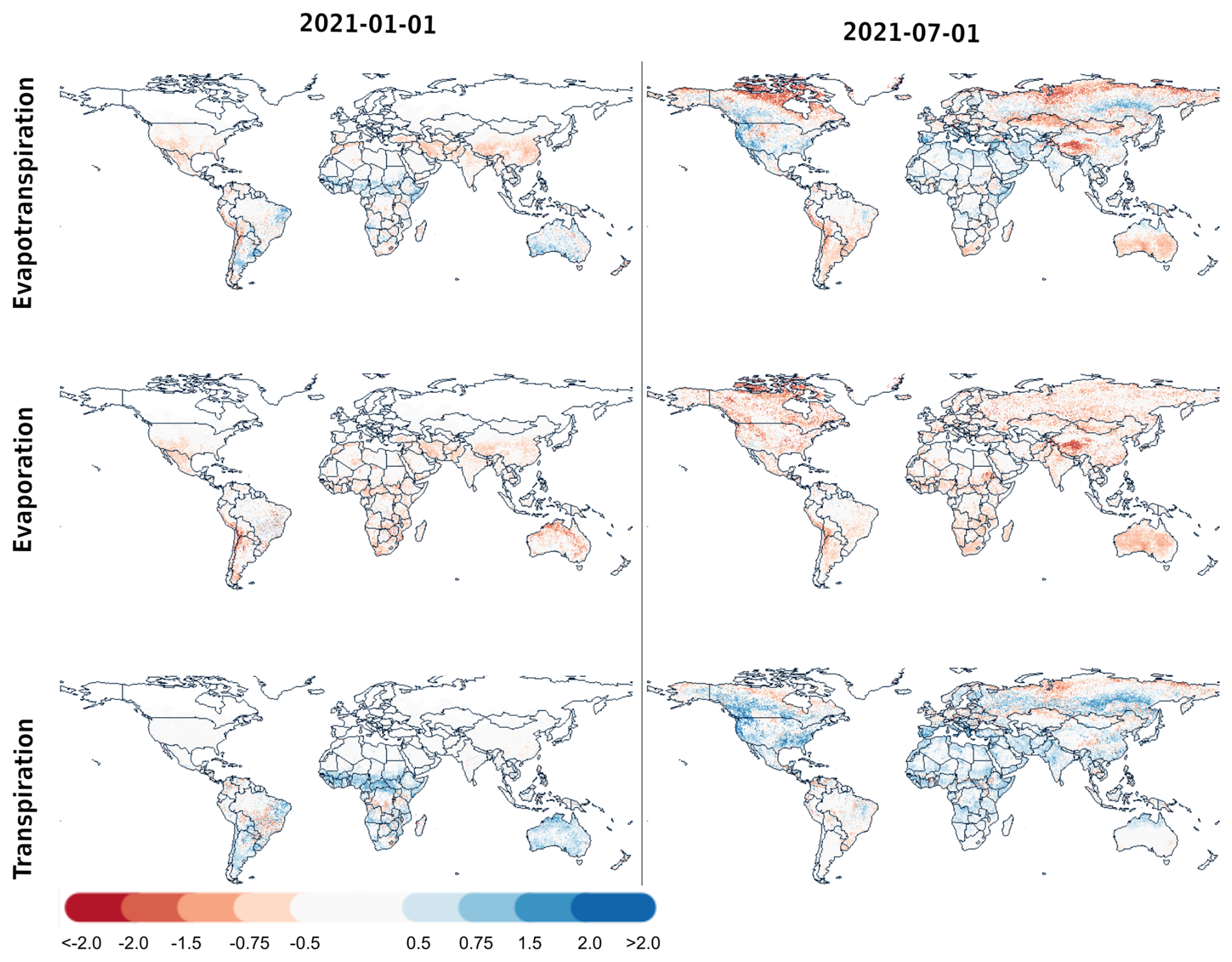
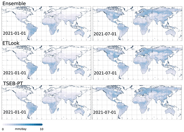
Figure 10Differences (ETLook − TSEB-PT: mm d−1) between estimates of ET, E and T of the two models on the first dekad of January and July 2021.
The global distribution of differences between the two models during two selected dekads (northern hemisphere winter and northern hemisphere summer) can be seen in Fig. 10 with absolute bias and values of ET on the same dekads shown in Appendix C (Figs. C5 and C6 respectively). A complementary view of the differences and similarities between the two models is also presented in Appendix C (Fig. C7), which shows histograms of the dekadal ETa values (for the same two dekads) as modelled by ETLook and TSEB-PT for a number of 10° lat/lon tiles capturing different climatic zones.
Looking at the figures it is clear that the differences between ETLook and TSEB-PT are more pronounced in July. This is expected as northern hemisphere summer is the main global growing season and thus the magnitude of the fluxes is the largest. During January the main differences appear in savannas, shrublands and grasslands in the southern parts of the globe, e.g. Sahel and southern Africa, parts of Brazil and Argentina and Australia. In those areas, ETLook yields higher ET values due to a higher estimation of transpiration by that model. Observable differences, but of smaller magnitude, are also present in a band spanning latitudes of around 20 to 40° N and the Andes, where TSEB-PT produces higher ET values due to higher estimation of E. In July the picture is mixed with larger ET estimates by TSEB-PT at both higher latitudes (both northern and southern) and higher altitudes (e.g. Tibetan plateau and Andes), and ETLook estimating higher rates in semi-arid areas. The higher ET estimated by TSEB-PT can be mainly attributed to higher evaporation estimates by that model, and conversely higher ET estimates by ETLook can be attributed to higher transpiration estimates. In tropical rainforests (Amazon, Congo, Borneo) and agricultural areas (e.g. central and eastern Europe, parts of India and China) the differences between the ET (and E and T) from the two models are minimal in both dekads.
The above observations are supported by the tower-based validation results in Sect. 3.2. It was demonstrated that ETLook and TSEB-PT generally achieve similar performance, and that the main differences emerge in dry climates and forests in temperate and continental climates.
Dry climate regions and savannas sites (SAV, WSA) were generally characterized by a stronger positive bias in ETLook, compared to TSEB-PT. Furthermore, TSEB-PT displayed higher correlation and lower RMSE than ETLook. Still, the Ensemble was generally outperforming TSEB-PT. Those regions are water, not radiation, limited and therefore in ETLook the soil moisture stress factor plays an important role. Previous studies have shown that the WaPOR ETa dataset, based on the same ETLook model implementation as used in this study, tends to overestimate ET in such regions due to likely overestimation of the internally derived soil moisture (Blatchford et al., 2020; Cogill et al., 2025). Those studies also highlighted the difficulty of ETLook in capturing the ET dynamics in tropical (humid) regions due to poorer performance of Penman–Monteith based models in areas with low vapour pressure deficit. This can be observed in the current study too with much lower correlation of ETLook in tropical climate compared to TSEB-PT, despite having comparable RMSE and (to smaller extent) bias in this climate.
In forest sites (DBF, ENF, MF), ETLook in general showed higher variability (standard deviation) of fluxes and closer to that of flux-towers, resulting in a higher accuracy. In most cases (DNF, EBF, ENF) the Ensemble performed better than the two individual models but in DBF and MF ETLook showed the best overall model performance. The lower performance of TSEB-PT in those cases might be caused by two reasons: (i) its relative higher sensitivity to canopy height (Burchard-Levine et al., 2020), and (ii) its dependence of a first-guess potential transpiration based on the Priestley-Taylor parameter, which in case of broadleaved and needleleaved forests might deviate from (respectively) the fixed value of 0.82 and the empirical relationship with canopy height described by Komatsu (2005). In deciduous needleleaved forest (DNF) in particular the bias and RMSE of TSEB-PT is much higher than that of ETLook and this could point to poor applicability of Komatsu (2005) relationship in that type of forest caused by only two out of 45 needeleaved sites used to derive it being located in this PFT.
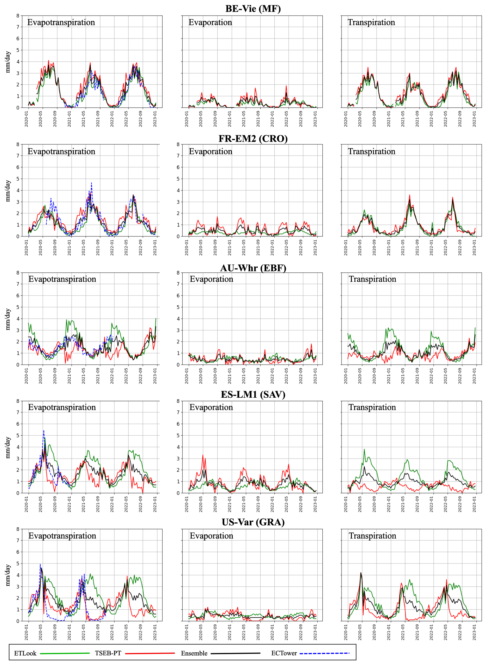
Figure 11Dekadal ET, E and T as modelled by TSEB-PT and ETLook and Ensemble product and dekadal ET from the eddy covariance towers in five validation sites covering different PFTs. The Tower line represents EBC corrected value.
Looking at the timeseries of selected sites (Fig. 11), covering different PFTs, again supports the above conclusions. At the two of the sites where TSEB-PT and ETLook show similar performance against in-situ measurements (MF BE-Vie and CRO FR-EM2) both models also show very good agreement in the T estimates, although at the FR-EM2 site the E estimate of TSEB-PT is significantly higher than that of ETLook. Conversely, at the three sites where models show divergent behavior against EC measurements (EBF Au-Whr, SAV ES-LM1 and GRA US-Var), there is a large disagreement in T estimates with ETLook producing significantly higher values. In addition, at ES-LM1 the E estimate of TSEB-PT is significantly higher and at both ES-LM1 and US-Var the temporal patterns of E produced by the two models are inverted (TSEB-PT shows higher values in winter and spring and ETLook shows higher values in summer). In case of ES-LM1 and US-Var, TSEB-PT is able to capture a sudden drop of ET, which could be a result of agricultural practices or dry conditions, while ETLook continues to estimate high T and ET for the duration of the growing season. On the other hand, at AU-Whr TSEB-PT models a similar drop in ET and T, which results in negative correlation with tower measurements, while ETLook overestimates ET and T but captures well the relative temporal changes. Finally, Au-Whr and ES-LM1 are good examples in which the errors of the two models cancel each other out in the Ensemble dataset that results in good agreement with EC measurements, while in US-Var the Ensemble shows worse performance compared to TSEB-PT outputs.
Detailed attribution of the behavior described above to the different model assumptions and formulations is beyond the scope of this study. However, some general observations can already be made. Firstly, the partition of ET into E and T is to a large extent guided by the partition on net radiation into the soil and canopy components respectively. Here, TSEB-PT employs a more complex radiation transfer model (Kustas and Norman, 1999; Campbell and Norman, 1998) that accounts for differential spectral behavior in the PAR, NIR spectral regions, while ETLook relies on a simpler partition based on LAI and Beer-Lambert law (FRAME Consortium, 2024). In addition the longwave component of net radiation (Ln) is also computed differently. In the TSEB-PT model, Ln is computed according to Eq. (2a) from Kustas and Norman (1999) using CAMS “surface thermal radiation downwards” field together with internally computed leaf and soil temperatures, constant emissivity values for the leaf and soil components (0.98 and 0.95 respectively) and effective leaf area index. ETLook estimates it following the FAO-56 approach and daily values of air temperature, vapour pressure and transmissivity (FRAME Consortium, 2024).
Another aspect is the partition of the net radiation of soil and canopy into latent and sensible heat fluxes (and ground heat flux in case of soil). In TSEB-PT the transpiration is initially assumed to be at the potential rate and this is later throttled down if invalid values of other fluxes are obtained (see Sect. 2.1.1). In forests the potential ET is set to a lower values, depending on forest height and type, based on the empirical model developed by Komatsu (2005). This model might not be applicable to all the different forest types and during all phenological stages which might lead to low variability (standard deviation) of the observed fluxes in most forest classes (see Fig. C3). Taking AU-Whr as an example, it is an open eucalyptus forest and classified as evergreen broadleaved forest and thus assigned a constant αPT parameter of 0.82. However, this value might not capture the different transpiration rates of the understory or specific adaptations of tree-grass ecosystems in dry climates. In the TSEP-PT model, evaporation is estimated as a residual of the other fluxes. For example in FR-EM2 TSEB-PT E has high values in spring and autumn, leading to overestimation of TSEB-PT ET during those seasons, and this could be caused by increased uncertainty in modelling the other energy fluxes of the soil at the time when it is exposed.
In ETLook the partition between latent and sensible heat fluxes of soil and canopy depends on the environmental stress factors and resistances which are based on meteorological and structural conditions as well as soil moisture (SM). The soil moisture is derived using LST (see Sect. 2.1.2) and therefore in vegetated conditions (when satellite mainly observes the canopy) it is more closely connected to root-zone moisture while in bare soil conditions it is connected mainly to top-soil moisture. However, the same SM estimate is used for both E and T calculations and therefore could lead to increased uncertainty of E or T depending on the canopy cover. In Fig. 11 it can be observed that T is overestimated in the three sites located in arid conditions (AU-Whr, ES-LM1 and US-Var) which could point to problems with the root-zone SM estimation in such conditions. The evaporation estimated by ETLook tends to display both low variability and low values. This again could be linked to uncertainties in the estimation of top-soil moisture and to the use of constant parameterization (regardless of soil type) when calculating soil resistance (Eq. 8).
Since the two ET models take different approaches, with different assumptions and approximations, they perform differently in various PFTs, climates and even phenological stages. The Ensemble (average) of the two provides more accurate ET than either of the models in most cases due to cancellation of random (and sometimes systematic) errors. However, there are also sites and PFTs where individual models might obtain better accuracy statistics. Therefore, as part of the CLMS ETa product users have access to individual TSEB-PT and ETLook model outputs as well as the Ensemble dataset. In addition, per-pixel standard deviation between the dekadal ET estimated by the two models is also included in the product as an ancillary quality layer since it can provide information on the uncertainty of the ET estimates due to model formulations. Finally, the TSEB-PT model also produces instantaneous latent and sensible heat fluxes which are available as part of the CLMS ETa product. Those heat fluxes do not undergo gap-filling and are distributed with a daily time-step and therefore might be preferred for applications such as fire risk/spread monitoring which are time-critical and in which gap-filling might produce increased uncertainty due to potential of significant changes at the land surface.
4.2 Comparison with WaPOR and OpenET ETa products
WaPOR global ETa dataset is the only existing operational and global ETa product with specifications very similar to the CLMS ETa. Furthermore, given the particular interest of FAO in the quality of the upcoming CLMS ETa product, WaPOR dekadal ETa values (WaPOR Level 1 version 3 – https://data.apps.fao.org/catalog//iso/7f4a7339-d56e-4393-8712-a8ffeffe2731, last access: 4 August 2025) were extracted for the study sites and timeslots and included in the analysis presented in Table 10. Based on those figures, the accuracy of the CLMS Ensemble ETa is significantly improved compared to WaPOR ETa (especially bias), while the individual model runs of TSEB-PT or ETLook have smaller bias but slightly lower correlation than WaPOR. It is also worth noting that the bias values of TSEB-PT and the Ensemble ETa are positive whereas ETLook and WaPOR exhibited a negative bias.
Table 10Bias (modelled − measured: mm d−1), Root Mean Squared Error (RMSE: mm d−1), and Pearson correlation coefficient (r) scores for dekadal ET for the CLMS products and WaPOR. rRMSE and rBias are the relative RMSE and relative Bias (i.e. RMSE and Bias divided by mean measured ET).
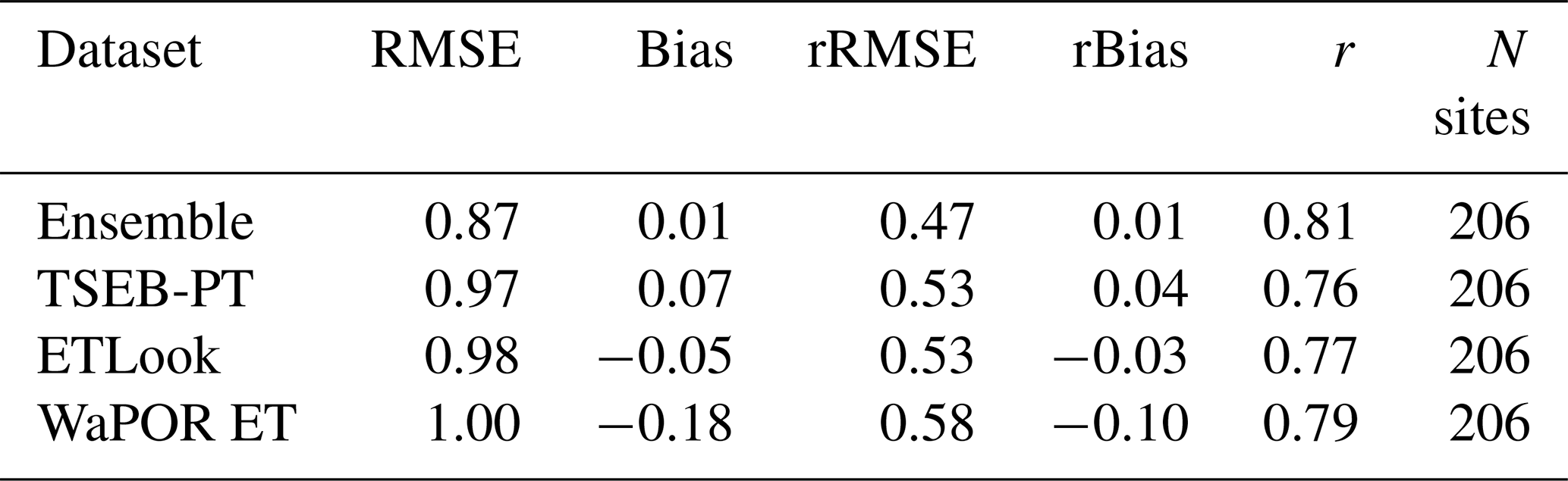
When comparing global spatial patterns (Fig. C8), it can be observed that compared to the CLMS datasets, WaPOR generally produces higher T estimates and lower E estimates. As expected the differences are smallest when comparing ETLook and WaPOR since the model setup should be fairly similar (the operational production setup of WaPOR is not public although FAO has created equivalent open-source package which produces similar results when run with the same input data). Therefore, the differences can be attributed mainly to the input data. Here, four possible reasons appear likely:
-
While CLMS relies on DMS to improve the spatial resolution of 1 km Sentinel-3 LST, WaPOR (version 3) uses the LST observations acquired by the VIIRS sensor on board of Suomi-NPP satellite with 375 m spatial resolution.
-
The CLMS ETa dataset was produced in NRT mode, meaning that forecast meteorological forcing were used and gap-filling was performed using only preceding dates. On the other hand, historical WaPOR ETa used in this study is a reanalysis product which means that reanalysis meteorological forcing was used and gap-filling was performed using both preceding and succeeding dates.
-
WaPOR ETLook implementation relies of some temporarily-static – spatially-distributed layers which parameterize the model. Those layers were used in CLMS ETLook implementation whenever available but there are still some layers which are not publicly disclosed in which case default constant values were used.
-
WaPOR dataset explicitly separates evaporation from canopy interception into a sub-product while in the CLMS dataset (for both ETLook and TSEB-PT) it is bundled together with E.
OpenET (Melton et al., 2022) is another dataset with which CLMS ETa can be compared. Although OpenET is produced with much higher spatial (30 m) and temporal (daily) resolutions and only in the United States, similarly to CLMS dataset it contains a product which is an average (ensemble) of individual ET models (6 in case of OpenET). In a recent validation study, the RMSE of monthly ensemble product was between 12 % and 30 % lower than that of individual models while r2 increased from 0.83–0.87 for individual models to 0.9 for ensemble (Volk et al., 2024). In our case the RMSE of dekadal Ensemble product was 10 % lower than that of TSEB-PT and ETLook models, while r increased from 0.76/0.77 for individual models to 0.81 for Ensemble product. In another study, the daily mean Ensemble OpenET product had a RMSE of 0.96 mm d−1, bias of −0.2 mm d−1 and r2 of 0.84 (Melton et al., 2022) which is very similar to the results presented in Table 8 for the Ensemble dekadal ETa despite the increased uncertainty when validating 300 m product due to spatial-scale mismatch between flux tower footprint and pixels size.
Further comparison of CLMS ETa product, and its E and T components, and other global ETa datasets can be found in Sect. 4.5 of the product Validation Report (Barrios et al., 2025).
4.3 Evaluation of CLMS ETa modelling framework components
Section 3 focused on the validation of the final CLMS ETa model outputs. During the development of the ETa modelling framework various design choices were made and intermediate products evaluated to justify those choices. In this section, we briefly present this evaluation.
4.3.1 Biophysical traits, albedo and net shortwave radiation
The biophysical traits were obtained by random-forest inversion of PROSPECT-D+4SAIL RTM (Sect. 2.2.2). In order to test the sensitivity and robustness of such inversion method, we ran an independent set of PROSPECT-D+4SAIL simulations to compare how the regression model predicts the biophysical traits. Random white noise was added to this test dataset, considering that retrieved TOC have relative uncertainty of 10 % (). This is shown as an example in Table 11.
Table 11Evaluation performance for the Random Forest hybrid inversion of the PROSPECT-D+4SAIL radiative transfer model. The “observed” dataset corresponds to 40 000 independent simulation of PROSPECT-D+4SAIL for a VZA = 0°, SZA = 37.5°, a standard atmosphere, and a relative uncertainty of 10 % in the TOC reflectance retrievals. Cab, Car, Ant, Cbrown, are respectively the leaf concentrations of chlorophyll a+b, carotenoids, anthocyanins and brown pigments; Cm and Cw are respectively the leaf dry matter and water contents; LAI is the leaf area index and Leaf Angle is the Campbell (1990) mean leaf inclination angle. Physical units in the error metrics are consistent with those on Table 4.
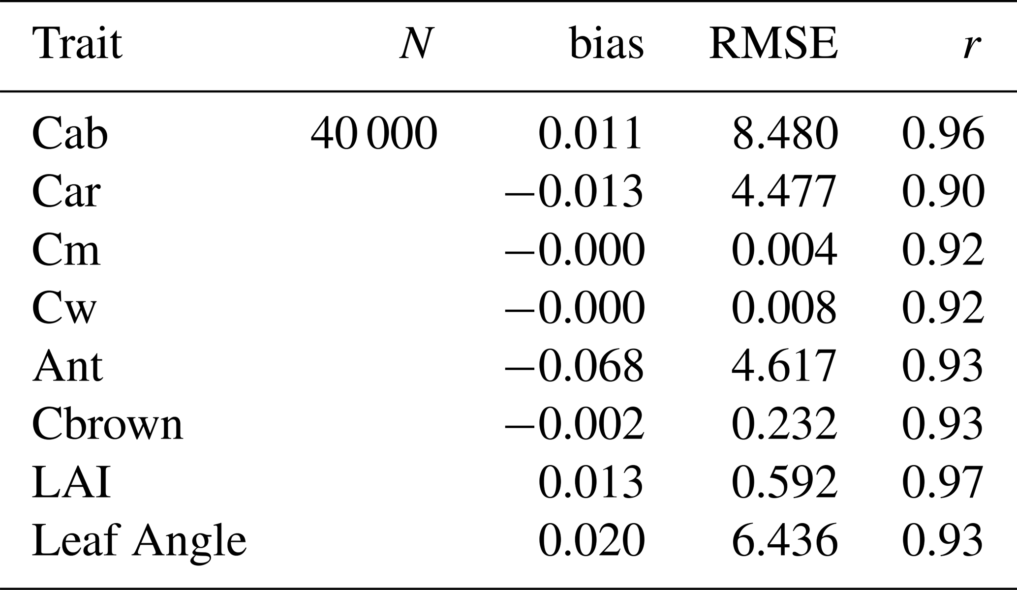
A more computationally efficient alternative for the retrieval of LAI and fg (but not pigments used for albedo estimation) would be to use the daily estimates of LAI and fraction of absorbed photosynthetically active radiation (fAPAR), which are internal CLMS datasets used to produce the 300 m dekadal biophysical CLMS product. In this case we could use a simple relationship between fg, LAI and fAPAR (Fisher et al., 2008) in order to derive the fraction of LAI that is green (fg).
where LAI is the total Leaf Area Index , fIPAR is fraction of intercepted photosynthetically active radiation and K(θs) is the shortwave beam coefficient of extinction at solar zenith angle θs.
Since CLMS LAI product actually represents the green LAI (Copernicus Land Monitoring Service, 2022), and with fg and total LAI unknown, an iterative procedure proposed by Guzinski et al. (2020) is performed to find the optimal value of fg based on gLAI and fAPAR. An initial LAI is assumed equal to gLAI (i.e. fg=1), from which fIPAR is computed from Eq. (20) and then fg recalculated with Eq. (19). This process is repeated until the fg value converges between iterations.
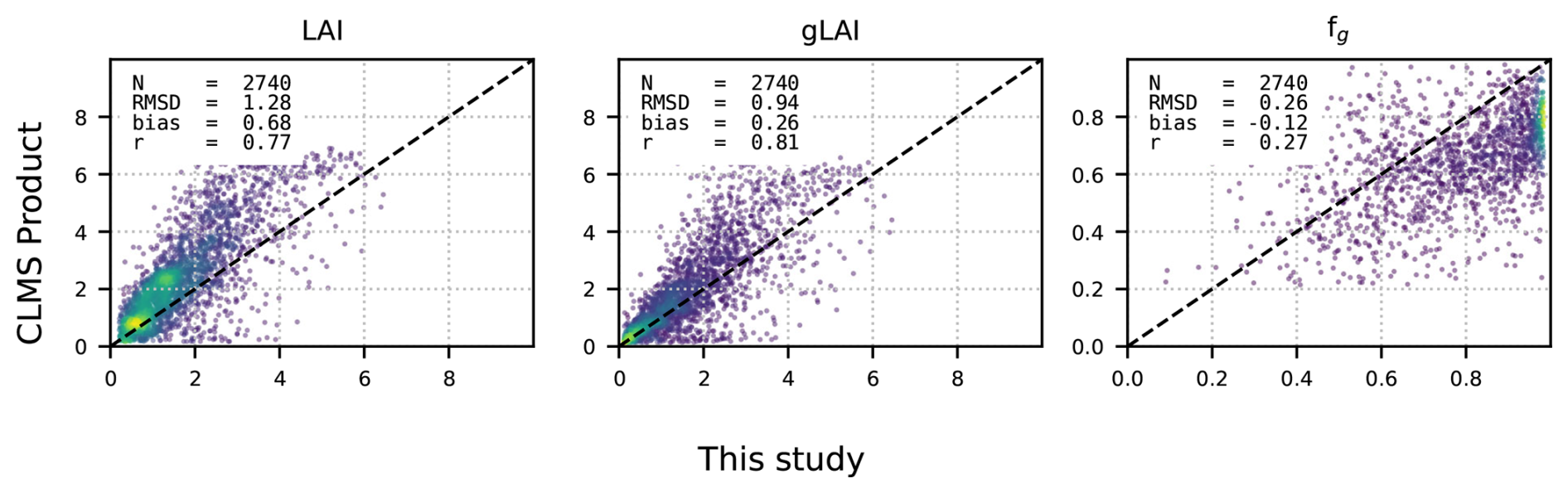
Figure 12Density scatterplot intercomparison between the biophysical processor LAI, green LAI (gLAI) and fg (x-axis) and those derived from the alternative use of CLMS LAI/FAPAR 300 m global products, version 1 (y-axis).
In order to evaluate whether both approaches provide consistent data, we ran the biophysical processor over sites included in the ICOS WarmWinter2020 database (Warm Winter 2020 Team et al., 2022). These selected sites are listed in Table B5. We thus compared both LAI and fg retrieved between 2019 and 2021 using the method described in Sect. 2.2.2 against the Fisher et al. (2008) and Guzinski et al. (2020) LAI/fAPAR approach using the CLMS FAPAR (Copernicus Land Monitoring Service, 2017a) and LAI (Copernicus Land Monitoring Service, 2017b) global products at 300 m, version 1. The density plots of Fig. 12 shows that overall the LAI products agree well, in particular at values lower than 2–3, with best agreement for green LAI (gLAI). Nonetheless, the larger scatter at higher LAI (i.e. denser vegetation) is not of great concern, as over these very dense canopies the interception (transmission) of radiation is already close to the maximum (minimum), i.e. near the light saturation, and thus these uncertainties have a minimal effect on ETa modelling. It is worth noting these results do not evaluate whether any of the two approaches is better than the other. Indeed, the CLMS gLAI has been intensively validated with a wide dataset of in situ LAI measurements (Copernicus Land Monitoring Service, 2025a) and thus it can be trusted with great confidence.
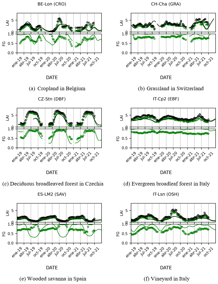
Figure 13Timeseries intercomparison between the LAI (in black), gLAI (in green in LAI sub-panel) and fg (in green in FG sub-panel) products retrieved from the biophysical processor (plain line) and those derived from the alternative use of CLMS LAI/fAPAR products (hollow circles).
However, the fraction of LAI that is green (fg) shows larger scatter and with the point cloud in Fig. 12 far from the 1 : 1 line. This deviation has indeed an effect on the comparison of total LAI with larger scatter and a slight positive bias towards the total LAI derived from the CLMS LAI/fAPAR. In order to better understand the different behavior of fg, Fig. 13 shows the timeseries for LAI, gLAI and fg over selected representative ICOS sites. These sites include both temperate and semi-arid conditions and a wide range of biomes: broadleaved and conifer forests, croplands, grasslands, savannas, and orchards/vineyards.
These timeseries confirm that LAI trends are mostly in agreement, with only some bias present in very dense vegetation: croplands during their peak development, broadleaved forests in summer and conifer forests. However, the behavior of fg shows discrepancies in certain cases. For instance, we would expect that herbaceous croplands (Fig. 13a) remain mostly green during the growing phase (spring) with fg values very close to 1 which then decrease during crop senescence in summer. However, thefg data derived from the CLMS LAI/fAPAR products shows values significantly lower than one during spring, and sometimes values close to 1 when LAI decreases during senescence. Another inconsistent behaviour was found in the savanna site (Fig. 13e), in which the CLMS LAI/fAPAR fg even shows an opposite trend as one would expect i.e. decrease of fg in late spring reaching a minimum in summer where most of the grass layer in this site is dead and only the evergreen oak canopy remains green and then a re-greening with the first rains of autumn. In addition, the fg derived with the CLMS LAI/fAPAR product seems to be also underestimated in the temperate grassland (Fig. 13b) and evergreen forest (Fig. 13d), as over these two temperate biomes the canopy should remain mostly green all year round.
PROSPECT-D model, through an emulator, was also used to derive leaf bihemispherical reflectances and transmittance (Sect. 2.2.3). The evaluation of the performance of this emulator is shown in Fig. 14. There is a larger scatter for the NIR reflectances and transmittances, likely due to the fact that we are intentionally excluding the PROSPECT-D leaf structural parameter, that basically controls the multiple scattering within the leaf tissues, which is of a larger magnitude in the NIR region than in the PAR. However, the uncertainties when deriving the reflectances and transmittances seem to be cancelled out when computing the leaf absorptance and therefore the conversion from pigments to leaf spectra seems sufficiently robust.
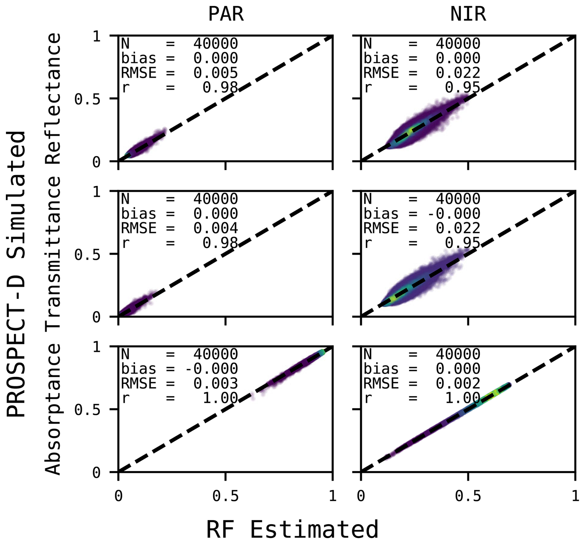
Figure 14Emulator of PROSPECT-D leaf radiative transfer model for the retrieval of broadband leaf reflectance, transmittance and absorptance factors.
To derive soil bihemispherical reflectance we converted narrowband reflectance values measured by Sentinel-3 satellites into broadband reflectance in PAR and NIR spectral regions using a linear regression approach (Sect. 2.2.3). We evaluated the goodness of this approach by running an independent set of simulations and compared the retrieved broadbands using the coefficients of Table 5. For both platforms, the evaluation confirms the robustness of conversion from the Sentinel-3 TOC reflectances to the broadband PAR, NIR and SW spectral regions, with negligible mean bias (≈ 0), very low RMSE and very good correlation (≈ 1) (Fig. 15).
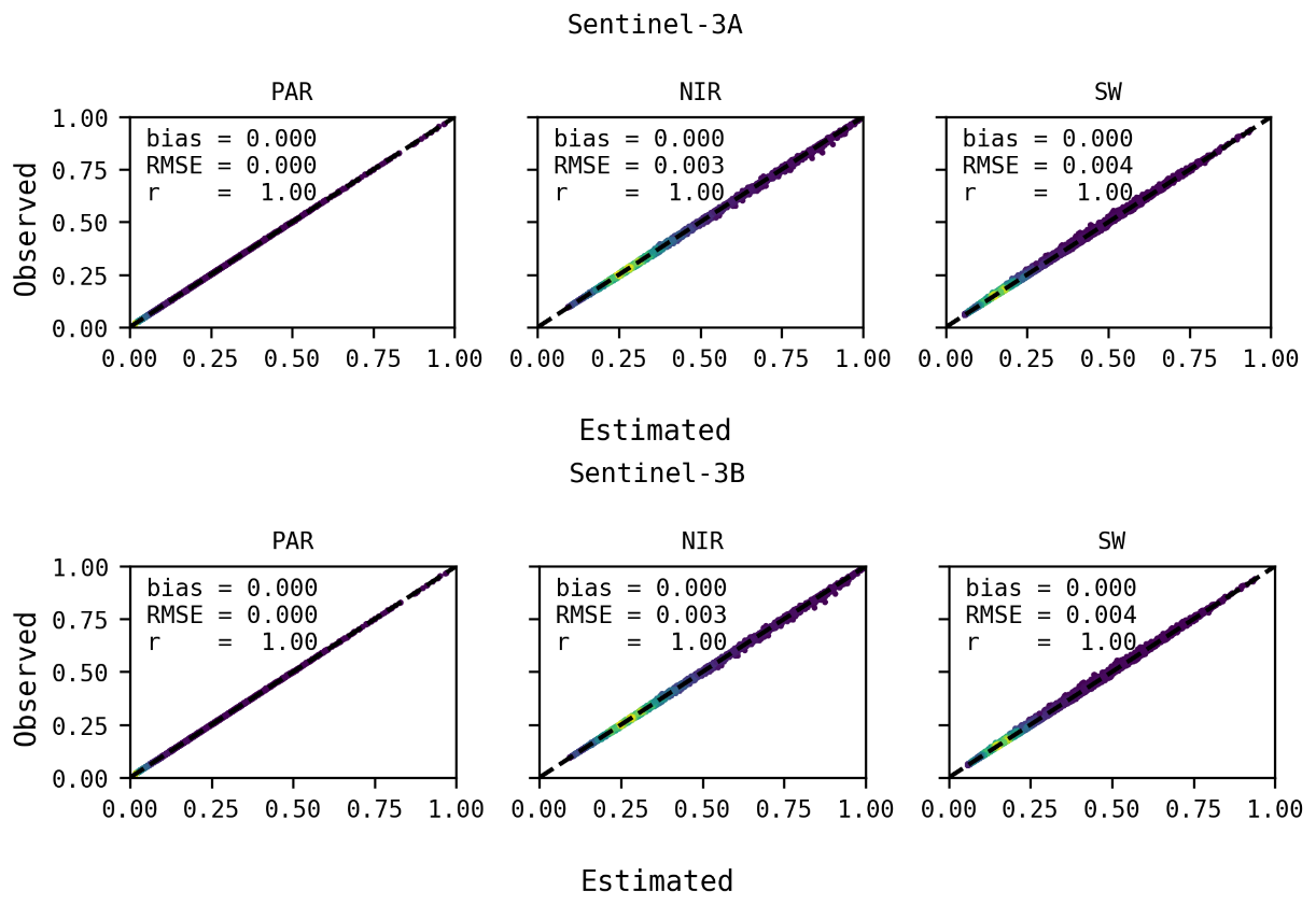
4.3.2 Land surface temperature sharpening
In the case of CLMS ETa product, the LST sharpening needs to be performed by a ratio of around 3 (i.e. from 1 km to 300 m). Because of this relatively small ratio, the sharpening could potentially be achieved with methods which are more computationally efficient than DMS. Therefore, we also evaluated the performance of a classic and simple (and therefore faster) sharpening method called TsHARP (Agam et al., 2007). It relies on finding a linear regression between the Normalized Difference Vegetation Index (NDVI) and LST. The regression is derived on the whole LST scene to be sharpened with NDVI resampled to the LST spatial resolution. Afterwards, the linear regression is applied to NDVI at its native resolution to estimate the representation of LST at this resolution. Finally, a bias correction step is applied to ensure the consistency of LST between the original and sharpened maps.
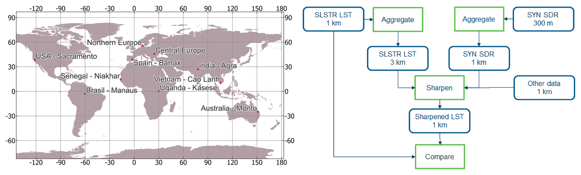
Figure 16Locations of areas of interest (left) and outline of the framework (right) used to evaluate DMS and TsHARP approaches for sharpening SLSTR LST images.
The two LST sharpening methods were tested in a number of geographically distributed areas of interest (AOI) covering different climatic zones and PFTs (Fig. 16 left panel) and across different seasons (images from at least four dates were sharpened at each AOI) to ensure a robust comparison. SY_2_SYN___ (SYN) Sentinel-3 product was used as a proxy for CLMS TOC reflectance product since the latter was still in production at the time this analysis was performed. The two products share the same spectral bands and spatial resolutions. The DMS regression models are trained on the entire Sentinel-3 SYN 3 min product data unit (PDU) (around 1400 km by 1200 km) as well as on subsets of 30 by 30 LST pixels in a moving window fashion. The evaluation of the sharpening methods was performed using the Sentinel-3 LST (as shown in Fig. 16 right panel) due to the lack of in situ LST data which could be used to validate satellite LST with 300 m spatial resolution. The SLSTR LST product was first resampled from 1 to 3 km and the SYN reflectance product was resampled from 300 m to 1 km, as was the ancillary data. The two sharpening methods were then used to recreate the LST at 1 km resolution, and the resulting map was compared with the original LST product. This evaluation framework assumes that there are no significant differences in relations between the explanatory variables and the LST when sharpening from 3 to 1 km and when sharpening from 1 to 300 m.
The results of the comparison are summarized in Table 12. At all sites the DMS method produces more accurate sharpened LST compared to TsHARP (see supplementary Table C2). The largest difference is at the Central Europe AOI where RMSE of DMS is up to 0.3 K lower than that of TsHARP and Mean Absolute Error (MAE) is up to 0.24 K lower. Looking at all sites, the RMSE of DMS is around 0.1 K lower compared to TsHARP (12 % difference) and MAE is around 0.06 K lower (10 % difference). Bias is minimal for both methods because bias correction is incorporated in both of them. Both methods also have similar and very high r2, with DMS being slightly better, and the slope of the linear regression between sharpened and original LST very close to 1.
Table 12Accuracy statistics for thermal sharpening: coefficient of determination (r2), Root Mean Square Error (RMSE), Mean Absolute Error (MAE), bias (modelled minus observed) and slope of the linear regression line between modelled and observed values. Model configurations are described in text.
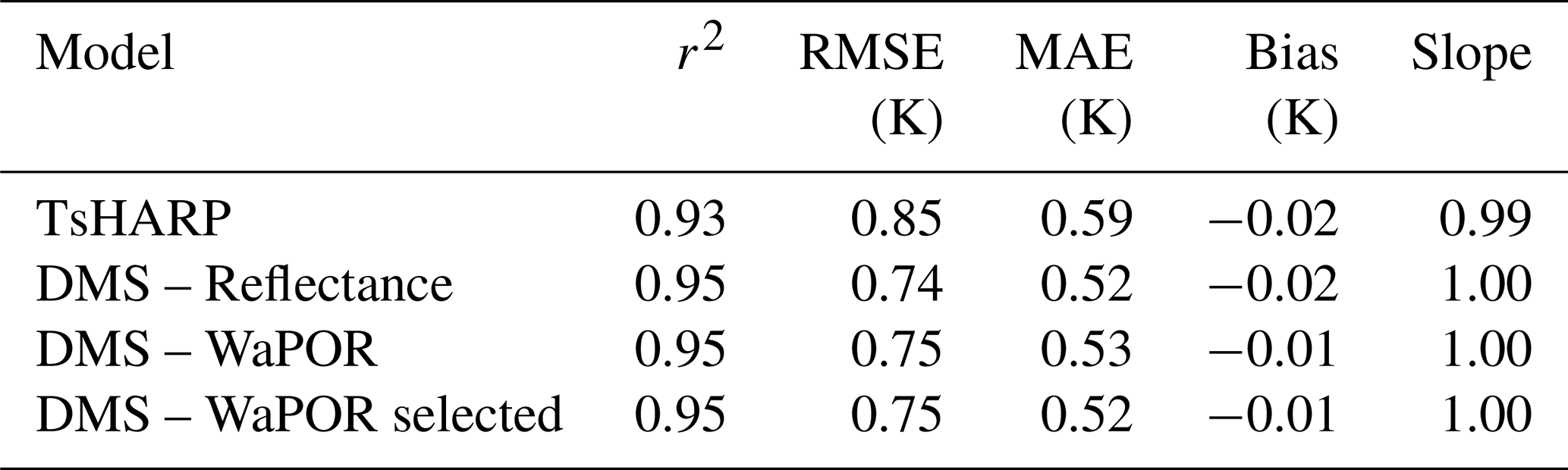
Regarding the three sets of DMS explanatory variables (see Sect. 2.2.4 for details), the differences between them are negligible. Looking at the details, there is no site in which “DMS – WaPOR” performs better than the other two configurations, while “DMS – Reflectance” has slightly better performance at some sites and “DMS – WaPOR selected” at others. However, the reduction in explanatory variables from 19 (“DMS – Reflectance”) to 9 (“DMS – WaPOR selected”) results in speed-up of the execution by a factor of around 2.3.
Qualitative assessment of the sharpened LST maps reveals that, in some cases, when variability of NDVI is low, TsHARP fails to find a meaningful relation between NDVI and LST (i.e. the linear regression has a slope close to 0). In such cases, the resulting sharpened LST is mainly an output of the bias correction step and has a blurry appearance consistent with simple resampling of lower resolution LST to higher resolution (see Fig. C9). In those cases, the quantitative analysis might still result in good accuracy statistics due to a small difference in spatial resolution between 3 and 1 km LST. DMS is less sensitive to, but not fully unaffected by, this issue because it relies on a range of spectral bands, indices, and DEM-based datasets. It is also noticeable that, in some cases, when there is insufficient information in the spectral data, DMS relies too heavily on DEM-based datasets, which can result in artifacts in the sharpened LST. One of the root causes of this issue could be the insufficient or incorrect atmospheric correction applied to SYN spectral bands. For operational production of CLMS ETa (and for production of data validated in Sect. 3) the SYN product is replaced by CLMS TOC reflectance product. The latter has shown improved agreement with in-situ measurements (Copernicus Land Monitoring Service, 2025c) and could therefore lead to an improvement in LST sharpening in such cases.
4.3.3 Weather forcing and ETa gap-filling
The suitability of the topographically corrected CAMS forecast data (Sect. 2.2.5) for modelling of actual evapotranspiration was assessed by comparing modelled daily solar irradiance and reference ET against measurements from 43 EC flux towers located in western Europe (France, Belgium, western Germany, Switzerland Spain, and northern Italy), United States and Australia (Fig. C10) for the year 2020. Those towers represent various topographical conditions from flat and low-lying to mountainous terrain as well as different climates, from arid to temperate. The statistical results of this comparison are shown in Fig. 17 and confirm the applicability of CAMS forecast for ETa modelling and suitability of the correction methods.
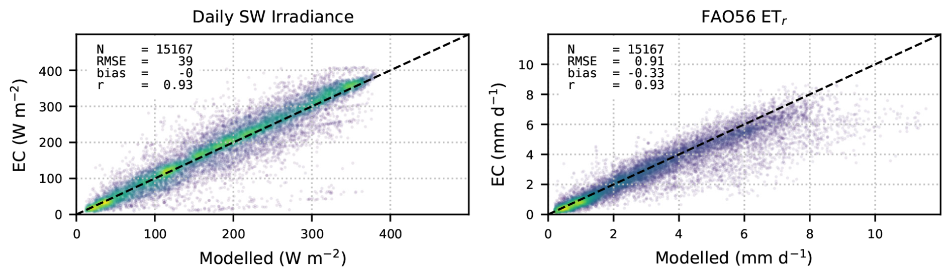
Figure 17Density scatter plots between daily solar irradiance (Daily SW Irradiance panel in W m−2) and reference ET (FAO56 ETr panel in mm d−1) modelled with topographically corrected CAMS forecast data (x-axis) and measured in 43 representative Eddy Covariance (EC) stations located in western Europe, United States and Australia (y-axis).
Apart from forcing the ET models, CAMS data was used for gap-filling of modelled ETa maps through the use of reference ET and precipitation (PR) (Sect. 2.3). We evaluated three gap-filling approaches: ignoring rainfall (called GFETr – Guzinski et al., 2021); taking rainfall into account as described in Guzinski et al. (2023) (called GFETr+PR); conservative modification of GFETr+PR described in Sect. 2.3 (called GFETr+PR80). We also evaluated near real-time (NRT) gap-filling periods with different maximum durations: 15 d (as used by default in Sen-ET approach), 30 and 60 d (as used in WaPOR during reprocessing). Finally, a non-time-critical (NTC) gap-filling with a maximum duration of 60 d (i.e. up to 60 d before and after target date) was also evaluated.
To evaluate the behaviour of the methods in diverse climates, we performed an analysis using in-situ ET measured at geographically distributed ICOS stations (Table B5). The daily ET at ICOS stations was calculated by summing up good quality instantaneous ET at hourly or half-hourly timesteps. Dates on which more than two measurements were of poor quality were ignored and no correction for lack of energy balance closure was performed. The determination of quality of ET data was based on ICOS quality flags associated with each measurement. Reference ET and rainfall sums were calculated from the stations' meteorological measurements. Cloudy days were identified as those for which measured solar irradiance was less than 80 % of theoretical surface solar irradiance in clear-sky conditions.
Table 13 presents the results on this evaluation. Statistics are calculated on daily basis and only for data points which were gap-filled and for which the rainfall adjustment is relevant. Neglecting rainfall can introduce an overall negative bias (underestimation) of up to −0.18 mm d−1 on wet, gap-filled dates. When rainfall is taken into account the introduced bias can become negligible and this reduction in bias leads to a less significant reduction in introduced uncertainty. Method GFETr+PR performs well with shorter window size but performance degrades significantly as window size increases and for largest windows the uncertainty is higher than for method GFETr. Method GFETr+PR80 results in lowest introduced bias and uncertainty with 60 d window size, chosen for the CLMS ETa processing chain. Finally, the NTC gap-filling performs better than NRT gap-filling and with method GFETr+PR80 performing the best in this case. An example timeseries of ET gap-filled with methods GFETr and GFETr+PR80 is shown in Fig. 18.
Table 13Accuracy statistics for gap-filling of evapotranspiration on cloudy days using ICOS in-situ data and different methods (described in text) and maximum window sizes (in NRT mode apart from last rows). Numbers highlighted in bold represent the best obtained statistics for each window size.
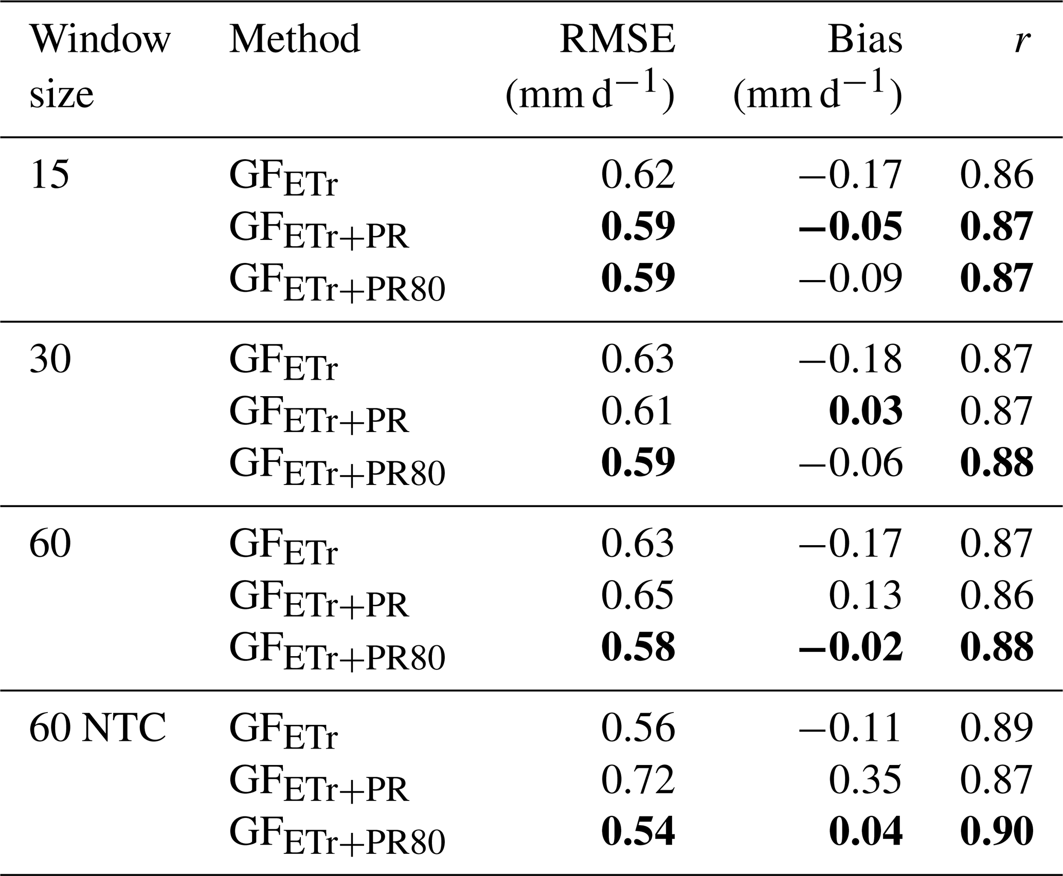
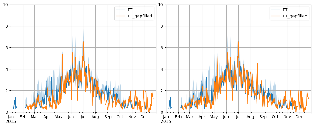
Figure 18An example of gap-filled ET timeseries at Voulundgaard ICOS station in 2015. Maximum gap-filling window of 60 d was used with, at left, gap-filling with rainfall not taken into account (method GFETr) and, at right, gap-filling with rainfall taken into account using the best performing method (method GFETr+PR80). Most notable differences are in spring (March–April) and late summer (July–August). Shaded area represents the uncertainty (energy balance closure error) of the data.
4.4 Limitations and potential improvements to the CLMS ETa product
The CLMS ETa product entered operational production at the end of 2025. Therefore, given the very short timeframe, it was not feasible to introduce changes for the initial version of the product. However, like most CLMS products, ETa might undergo evolution and reprocessing in the coming years and, therefore, it is worth to highlight some potential areas of improvement which might be the focus of this evolution.
One of the main limitations in producing medium- and high spatial resolution ET products (below 1 km) is the lack of LST observations with high spatio-temporal resolution, especially within the Copernicus Sentinel satellites. This situation should be resolved by the end of the decade when Land Surface Temperature Monitoring (LSTM) mission, with a primary objective of frequent monitoring of field-scale ETa, will join the Copernicus constellation (Koetz et al., 2018). In the meantime, it might be advantageous to make use of well established non-Copernicus sensors, such as VIIRS on board of Suomi-NPP satellite which can provide daily observations of LST with spatial resolution of 375 m.
Another potential improvement would be to compute a temporal running mean of biophysical parameters and TOC reflectance using the latest week of data. This should result in two benefits. Firstly, inverting the PROSPECT-D+4SAIL RTM (see Sect. 2.2.2) is an ill-posed problem, meaning that multiple combinations of biophysical parameters can result in the same reflectance. By taking a mean of multiple inversions, under the assumption that the biophysical conditions of vegetation do not change significantly over short time periods, the robustness of this inversion can be improved. Secondly, this will allow the full use of SLSTR swath with VZA below 35° by gap-filling the OLCI image on the eastern edge of the swath (see Sect. 2.2.1).
Producing a reanalysis dataset, e.g. two months after the completion of NRT production, might also lead to improvements in the accuracy of the CLMS ETa product. Firstly, because it would allow the use of ERA5 reanalysis meteorological data (Hersbach et al., 2020) instead of CAMS forecast as ET model forcing. The former has improved accuracy and increased spatial resolution compared to the latter and is therefore expected to result in more robust ET estimates. Secondly, gap-filling could be performed using 60 d both preceding and succeeding the target date which will result in less cloud gaps in the final ETa maps but also in improved accuracy (compare two bottom rows of Table 13).
Currently the Ensemble is created by simple averaging of the ET (and E and T) modelled by TSEB-PT and ETLook. However, the two models might not perform equally well, or be equally suitable, for all climates and PFTs (see Sect. 4.1). Therefore, following the approach being suggested for other ET model ensembles (Reitz et al., 2025) it might be advantageous to use the assessment of individual model performance and uncertainty in different conditions when creating the Ensemble dataset. Those two ET models were chosen based on preliminary analysis funded by European Commission which led in their explicit inclusion in the call for tenders for the CLMS ETa product (JRC/2023/OP/0273 – https://ec.europa.eu/info/funding-tenders/opportunities/portal/screen/opportunities/tender-details/13795). This however does not imply that they are the best performing models in all circumstances. Therefore, enlarging the ensemble member size with additional ET models, e.g. those included in the OpenET ensemble (Melton et al., 2022) or other models which were shown to be applicable globally such as ETMonitor (Zheng et al., 2022), can further improve the robustness of the CLMS ETa product in future evolutions.
Adding an explicit sub-product on evaporation from canopy interception (currently implicitly included in the evaporation sub-product) could be another development area. Modeling this component robustly and operationally is not a straightforward task as the currently existing semi-empirical methods might not account for all the complexities of this process. Therefore, a novel multi-source energy balance model might need to be developed.
The modelling of evaporation of inland water bodies can be important for many applications, such as water resources management or SDG reporting. Therefore, a post-processing step could be introduced in which this flux could be estimated, e.g. using Penman model (Monteith and Unsworth, 2013) parameterized for water.
Finally, the implemented ET modelling workflows present some limitations compared to the state-of-the-art in ET modelling research, particularly in some climates and PFTs as discussed in Sect. 4.1. There are multiple studies looking into different aspects of ET modelling including more detailed radiation partitioning (Ponce De León et al., 2026), accounting for multiple sources of heat fluxes (Mwangi et al., 2022), improved estimation of aerodynamic resistances (Li et al., 2019) and surface roughness (Alfieri et al., 2019) and integration of direct soil moisture estimates into ET models (Huang et al., 2025). In an operational and global product there is an inherent trade-off between keeping up to date with latest research and maintaining consistency and accuracy in a global context within reasonable computational costs. The current version of the CLMS ETa product is the result of such trade-off analysis, assessing the potential pros and cons of research findings for a global product, executed within tight budget and time constraints. Upcoming evolutions will provide opportunities to re-assess this, guided by user feedback and new scientific developments.
In addition to the potential input data and model improvements presented above, the validation methodology could also be extended. The focus of this study was on point validation using EC sites spread around the globe. Despite our best efforts, there are still large areas (especially in Asia, Africa and South America) from which no EC measurements are available. In such areas, other quality assessment methods could be performed (Tran et al., 2023), including catchment scale water balance (Blatchford et al., 2020; Weerasinghe et al., 2020; Comini De Andrade et al., 2024), and statistical analysis of consistency and uncertainty using other global or regional products (He et al., 2025).
A global and operational actual evapotranspiration (ETa) product was introduced to the portfolio of the Copernicus Land Monitoring Service (CLMS) at the end of 2025. This addition is motivated by a request from the Food and Agriculture Organization of the United Nations but the new product will have a multitude of applications in water resources management, SDG reporting, food security, forest management and other fields. The product is designed to have a 300 m spatial resolution, dekadal (10 d average) temporal resolution for water fluxes (evapotranspiration and its components of evaporation and transpiration) and daily temporal resolution for instantaneous heat fluxes (latent and sensible heat), global extent and to be produced in near-real-time with 2 d delay (Table 1). As all other CLMS products, it is distributed with a free and open license and will have guaranteed long-term continuity.
The product is based almost exclusively on Copernicus data, ranging from imagery acquired by OLCI and SLSTR sensors on board of Sentinel-3 satellites through meteorological forecast data provided by Copernicus Atmosphere Monitoring Service (CAMS) to higher-level products such as land cover maps produced by Copernicus Land Monitoring Service (Table 3). Those data undergo significant pre-processing to turn them into input forcing (Table 2) for two ET models: TSEB-PT and ETLook (Sect. 2). The cloud masked top-of-canopy (TOC) reflectance from OLCI and SLSTR shortwave optical bands were obtained from CLMS TOC product, while LST from SLSTR thermal bands was based on the Sentinel-3 LST product. A decision was made not to gap-fill the cloud gaps in those input products since the TOC reflectances were acquired at the same time and location as LST and it was preferred not to gap-fill the latter in order to obtain most accurate energy balance at the surface. In addition, a maximum view zenith angle of 45° was enforced to limit uncertainty due to different directionality effects. The derivation of biophysical parameters (e.g. LAI, leaf pigments, fraction of LAI that is green, canopy albedo) was based on inversion of radiative transfer models driven by the TOC product spectral bands. This allowed us to obtain LAI comparable with the CLMS LAI product while at the same time to derive fraction of vegetation that is green which better aligns with the expected phenological patterns, and leaf pigments required for canopy albedo estimation. Applying efficient vectorization and inversion techniques allows even such complex approaches to be applied in NRT at global scale and daily timestep. Meteorological forcing was based on the CAMS forecast dataset and after undergoing rather simple topographical correction showed to be highly suitable for modelling of ET at 300 m resolution. The 1 km SLSTR LST product was sharpened to 300 m using Data Mining Sharpener, a complex machine learning method, and 300 m TOC product based spectral indices, reflectance and a DEM with a specific model trained and applied to each pair of scenes. The resulting LST recreates well the finer spatial details of the higher resolution although can also produce artifacts or blurry appearance when there is insufficiently strong relationship between the shortwave and thermal observations. Finally, the outputs of the two ET models were gap-filled using reference ET and rainfall to obtain all-weather ET estimates, with the latter adding important information on soil wetting and leading to improved accuracy of gap-filled ET. The selected input data are available globally and the pre-processing and ET gap-filling methods do not undergo any localized fine-tuning or specific parameterization and therefore are applicable globally (Sect. 4.3) and suitable as input also for other ET models.
A demonstration dataset of three years was produced using the prototype end-to-end processing chain for the CLMS ETa product and validated using three years of measurements from 206 globally distributed eddy covariance stations (Sect. 3). Despite our best efforts for EC data collection, there are areas of the globe which lack in-situ measurements and in which product performance is therefore more uncertain.
The two ET models individually proved to be capable of producing global ET estimates, both achieving RMSE below 1 mm d−1, correlation coefficient above 0.75, and absolute bias below 0.1 mm d−1 when compared to the in-situ measurements. Those results compare favourably with the WaPOR global ETa dataset produced by FAO, which has the same spatio-temporal characteristics as the Copernicus ETa products, and other higher-resolution ETa datasets (Sect. 4.2). However, when looking at different climates and plant functional types (PFTs), the differences between the model become apparent (Sect. 4.1). In particular ETLook model shows higher positive bias in semi-arid and arid areas, most probably due to the limitations of the LST – vegetation fractional cover trapezoid soil moisture estimation method. It also achieves lower correlation in tropical climate, possibly due to the underlying constraints of Penman Monteith model in humid environments. On the other hand, the TSEB-PT model struggles more in forested PFTs due to its higher sensitivity to vegetation height and unsuitability of default parameterization of Priestley-Taylor potential ET in forests. We tried to address those issues by using a LiDAR based vegetation height map and empirical correction factors but especially the latter could benefit from a more thorough physics-based approach.
Taking an ensemble (average) of the two models has shown to be an effective method to improve the ETa product performance. The Ensemble product achieved RMSE of 0.87 mm d−1, bias of 0.01 mm d−1 and correlation of 0.81 and outperformed the individual models in all climates and large majority of PFTs (Sect. 3.2). This was mainly due to cancellation of random and systematic errors when averaging the model outputs. However, in some circumstances either of the individual models outperformed the ensemble and therefore both individual model outputs and the ensemble values are distributed as part of the CLMS ETa product. A more intelligent method of creating the ensemble, based on specific model performances in different climate-PFT zones, as well as addition of new model members to the ensemble is expected to further improve product performance (Sect. 4.4).
The results of this study are highly encouraging for the production of global ETa dataset based on Copernicus data sources. The addition of operational and NRT ETa product in the CLMS portfolio should significantly enlarge the CLMS user community and encourage further development of applications leveraging ET maps from regional to global scales.
The direct-hemispherical spectral transmittance () at a given solar zenith angle (θS) is calculated following the equations of Campbell and Norman (1998) for a single layer canopy:
with λ being either the PAR or NIR. is the beam spectral reflection coefficient for a deep canopy with non-horizontal leaves (see Eq. A2), ζλ is the leaf absorptivity, κb is the extinction coefficient for direct-beam radiation (per LAI unit), and ρS,λ is the soil spectral reflectance. The multiple scattering between the soil and the canopy is accounted for in the and ρS,λ terms.
is the reflectance factor for a canopy with horizontal leaves.
Finally, the canopy beam extinction κb(ψ) is calculated based on the ellipsoidal LADF of Campbell (1990):
Diffuse spectral transmittance () is calculated by numerically integrating κb over the hemisphere:
and replacing κb by κd in Eq. (A1).
Similarly the canopy direct spectral albedo is computed as:
and the diffuse canopy albedo () by replacing κb(θS) by κd.
Tables B1, B2, B3 and B4 list all the EC flux tower sites used to validate CLMS ETa datasets. The ICOS datasets used in the analysis were the ETC L2 FLUXNET (ICOS RI et al., 2025) and the Warm Winter 2020 (ICOSww – Warm Winter 2020 Team et al., 2022). AsiaFlux site is described in Meijide et al. (2017). The DOIs of AmeriFlux sites are listed below:
-
CA-DBB: https://doi.org/10.17190/AMF/1881565 (Christen and Knox, 2025)
-
US-ARM: https://doi.org/10.17190/AMF/1854366 (Biraus et al., 2026)
-
US-Bi1: https://doi.org/10.17190/AMF/1871134 (Rey-Sanchez et al., 2025)
-
US-Bi2: https://doi.org/10.17190/AMF/1871135 (Rey-Sanchez et al., 2026)
-
US-BZF: https://doi.org/10.17190/AMF/1881570 (Euskirchen, 2026)
-
US-HB3: https://doi.org/10.17190/AMF/2229378 (Forsythe et al., 2026)
-
US-Jo1: https://doi.org/10.17190/AMF/1902833 (Tweedie, 2026)
-
US-Me6: https://doi.org/10.17190/AMF/2204871 (Hanson et al., 2026)
-
US-Mo1: https://doi.org/10.17190/AMF/2229382 (Schreiner-McGraw, 2026a)
-
US-Mo2: https://doi.org/10.17190/AMF/2229383 (Schreiner-McGraw, 2026b)
-
US-Mo3: https://doi.org/10.17190/AMF/2229384 (Schreiner-McGraw, 2026c)
-
US-ONA: https://doi.org/10.17190/AMF/1832163 (Silveira and Bracho, 2025)
-
US-Rls: https://doi.org/10.17190/AMF/2229387 (Flerchinger, 2026)
-
US-Ro4: https://doi.org/10.17190/AMF/1881589 (Baker and Griffis, 2026)
-
US-Ro5: https://doi.org/10.17190/AMF/1818371 (Baker and Griffis, 2025a)
-
US-Ro6: https://doi.org/10.17190/AMF/1881590 (Baker and Griffis, 2025b)
-
US-Sne: https://doi.org/10.17190/AMF/1871144 (Shortt et al., 2026)
-
US-SRG: https://doi.org/10.17190/AMF/2204877 (Scott, 2026a)
-
US-Ton: https://doi.org/10.17190/AMF/2204880 (Ma et al., 2026a)
-
US-Tw4: https://doi.org/10.17190/AMF/2204881 (Eichelmann et al., 2026)
-
US-Var: https://doi.org/10.17190/AMF/1993904 (Ma et al., 2026b)
-
US-Whs: https://doi.org/10.17190/AMF/1984574 (Scott, 2026b)
-
US-Wkg: https://doi.org/10.17190/AMF/1984575 (Scott, 2026c)
-
US-xAE: https://doi.org/10.17190/AMF/1985434 (NEON, 2025a)
-
US-xDC: https://doi.org/10.17190/AMF/1985437 (NEON, 2025b)
-
US-xDS: https://doi.org/10.17190/AMF/1985439 (NEON, 2025c)
-
US-xJE: https://doi.org/10.17190/AMF/1985443 (NEON, 2025d)
-
US-xSB: https://doi.org/10.17190/AMF/1985451 (NEON, 2025e)
-
US-xSE: https://doi.org/10.17190/AMF/1985452 (NEON, 2026a)
-
US-xST: https://doi.org/10.17190/AMF/1985454 (NEON, 2026b)
-
US-xTA: https://doi.org/10.17190/AMF/1985455 (NEON, 2026c)
-
US-xWD: https://doi.org/10.17190/AMF/2229412 (NEON, 2026d)
Table B5 lists selected sites from ICOS WarmWinter2020 database which were used to evaluate biophysical modelling and ET gap-filling approaches.
Table C1 and Fig. C1 show validation of modelled dekadal ETa (similarly to Table 8 and Fig. 7) but only against the flux towers for which ECB correction was applied.
Table B1Geographical location, climate region (Köppen classification), plant functional type (PFT) and network/dataset of origin for EC flux towers used for CLMS ETa model validation – part 1/4.
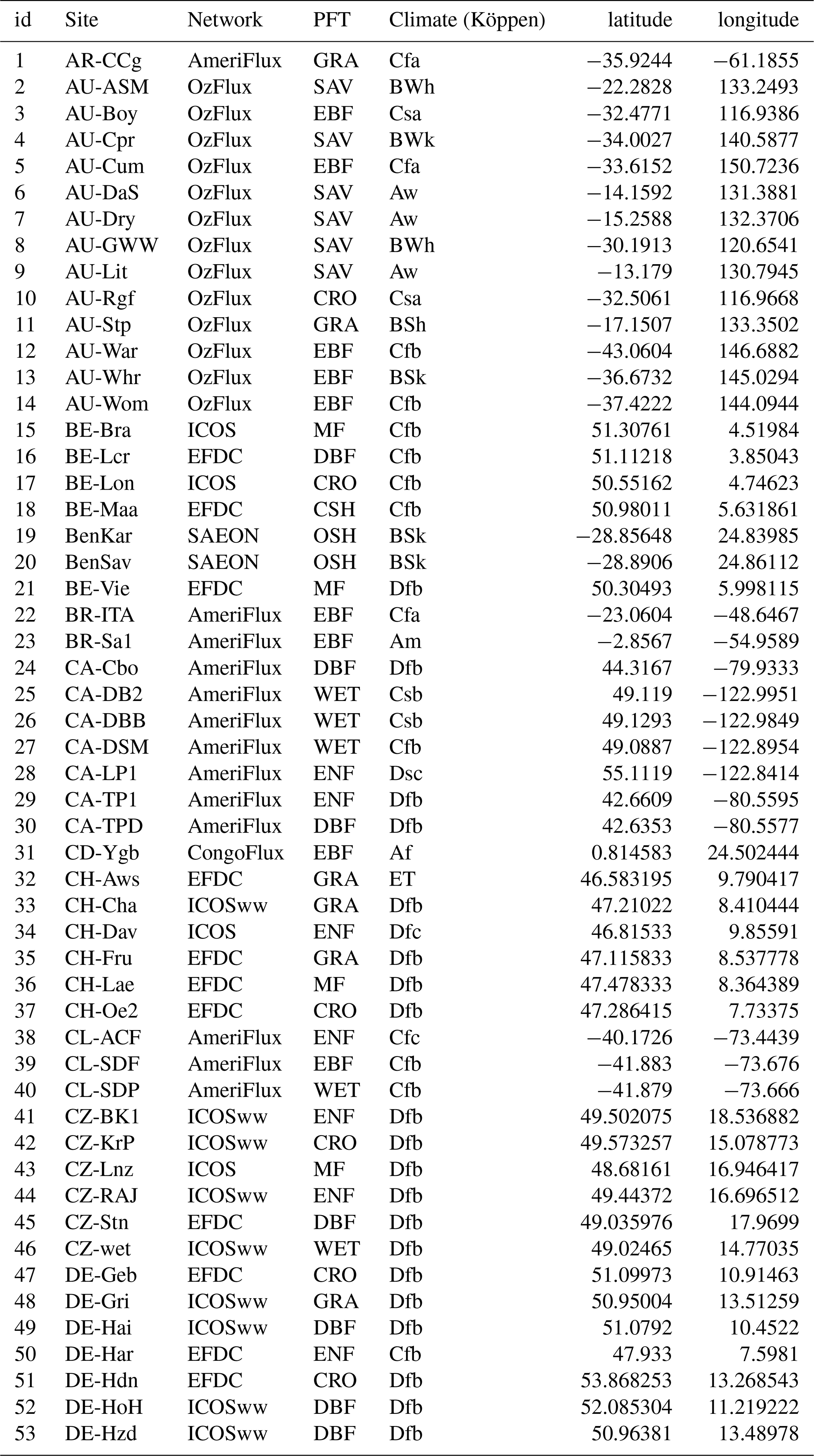
Table B2Geographical location, climate region (Köppen classification), plant functional type (PFT) and network/dataset of origin for EC flux towers used for CLMS ETa model validation – part 2/4.
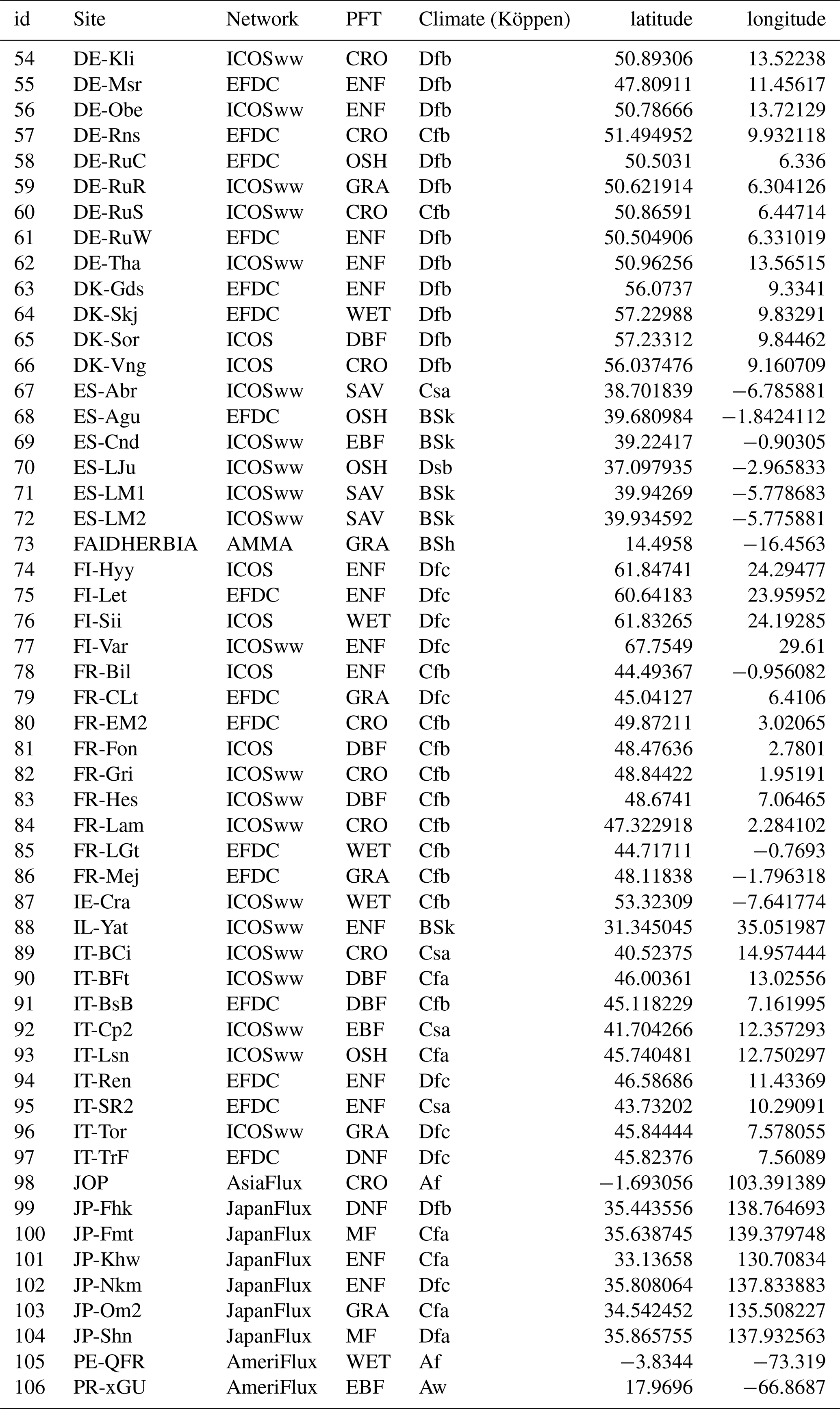
Table B3Geographical location, climate region (Köppen classification), plant functional type (PFT) and network/dataset of origin for EC flux towers used for CLMS ETa model validation – part 3/4.
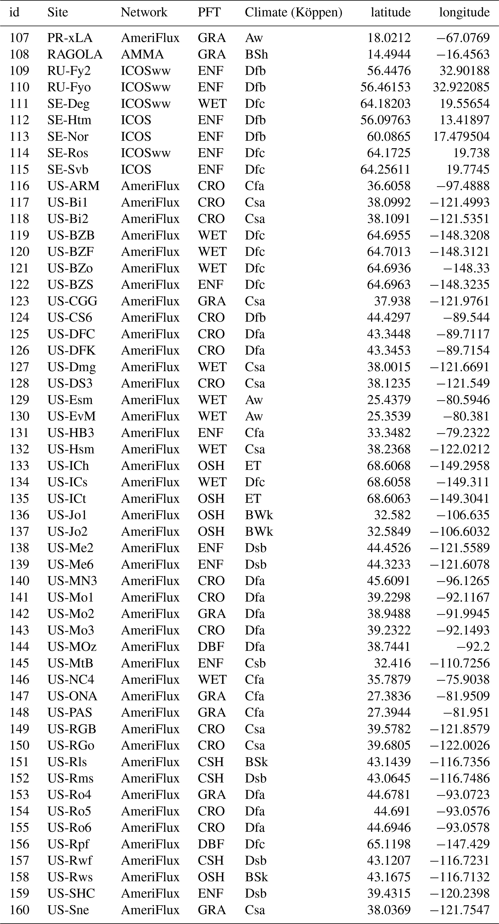
Table B4Geographical location, climate region (Köppen classification), plant functional type (PFT) and network/dataset of origin for EC flux towers used for CLMS ETa model validation – part 4/4.
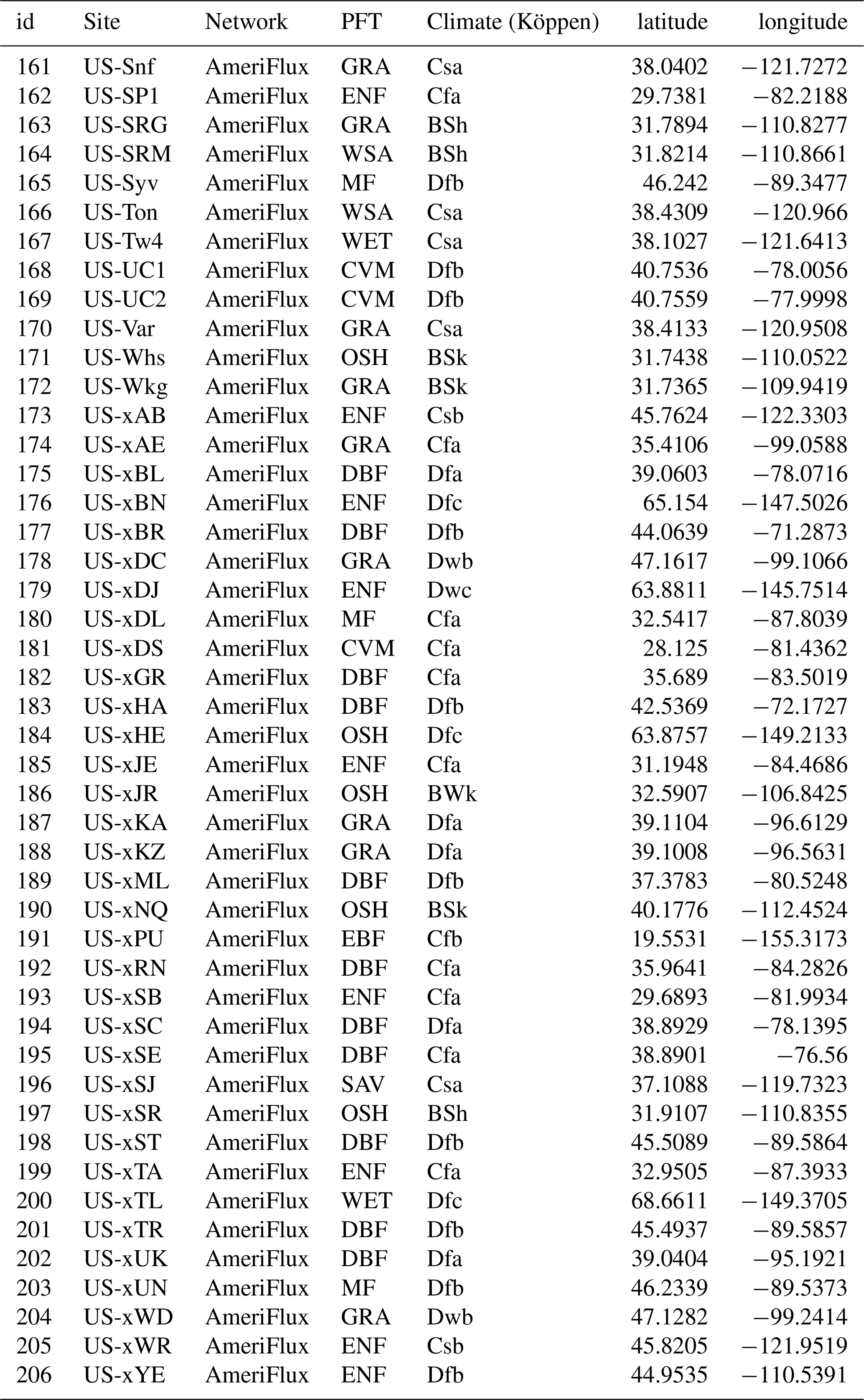
Table B5Selected sites from ICOS WarmWinter2020 database (Warm Winter 2020 Team et al., 2022) used to evaluate biophysical modelling and ET gap-filling approaches. In addition to geographical location the table shows climate region (Köppen classification) and plant functional type (PFT) of each site.
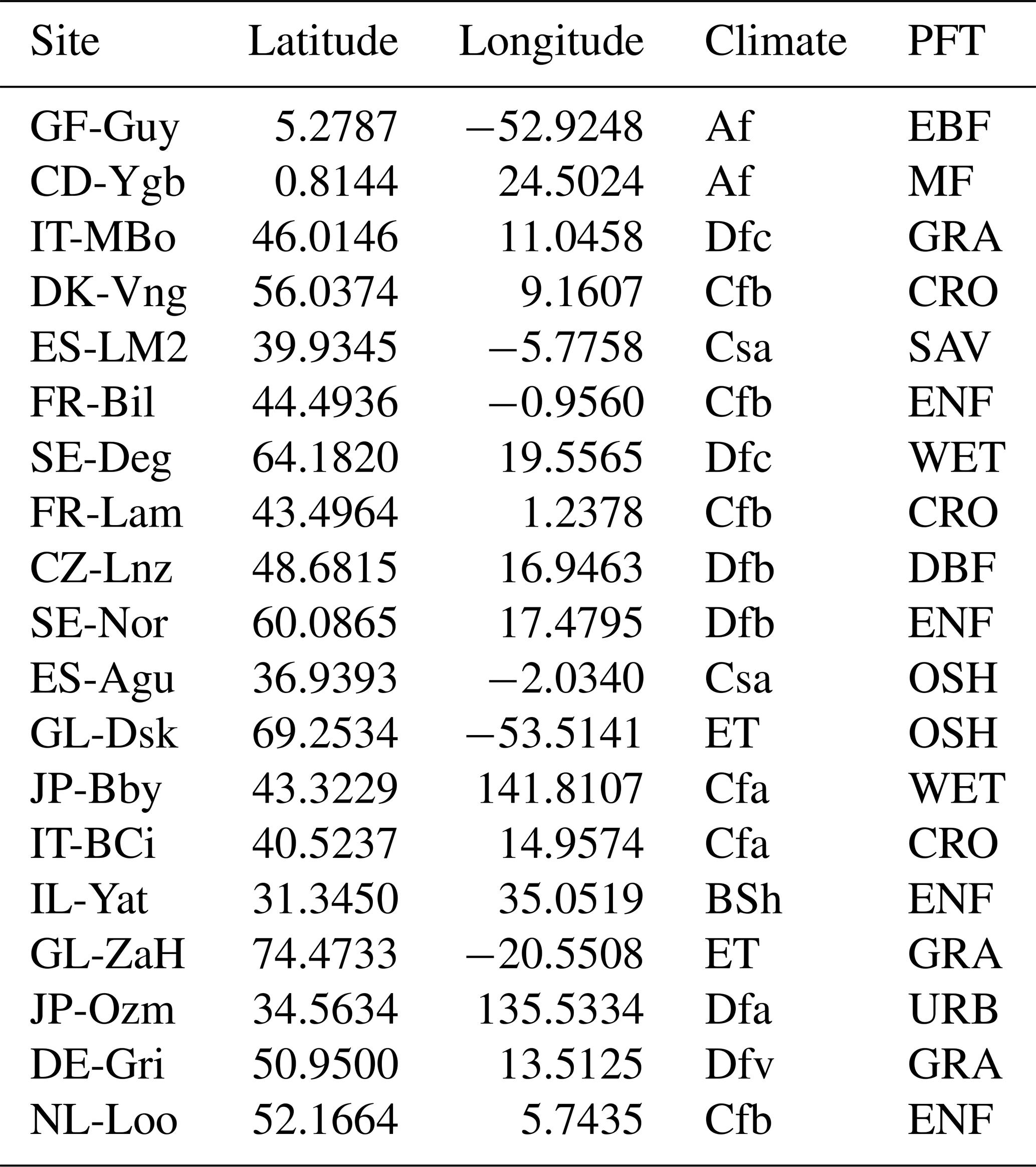
In this appendix we present supplementary figures and tables supporting the analysis conducted in the Sect. 3.2 (Validation results) and Sect. 4 (Discussion). Reader is referred to those section for more details.
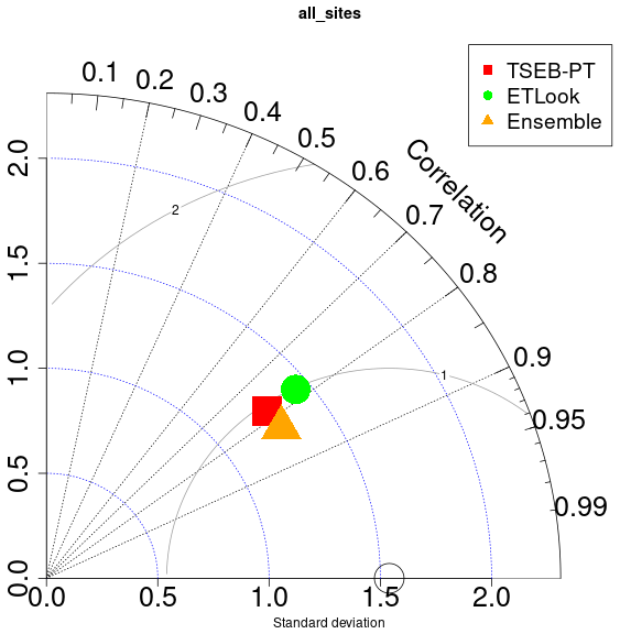
Figure C1Taylor-plot overview of dataset accuracies using only those sites in which energy balance closure (EBC) correction was applied (AmeriFlux, ICOS, OzFlux networks). Azimuthal angle represents the Pearson r, radial distance from the origin is the standard deviation (mm d−1). Circle marker at the horizontal axis represents perfect model performance, markers closer to this point indicate better model performance. Radial distance from this point is equivalent to centered RMSE (contour values shown in mm d−1). The statistics shown in the Taylor diagram were generated from the full dataset of observed and modelled ETa pairs across all EBC corrected validation sites.
Table C1Bias (modelled − measured: mm d−1), Root Mean Squared Error (RMSE: mm d−1), and Pearson correlation coefficient (r) scores for dekadal ETa per model (all sites combined), and summary statistics at site level for sites in which energy balance closure correction was applied (AmeriFlux, ICOS, OzFlux networks). rBias and rRMSE are relative metrics (i.e., divided by mean measured ET).

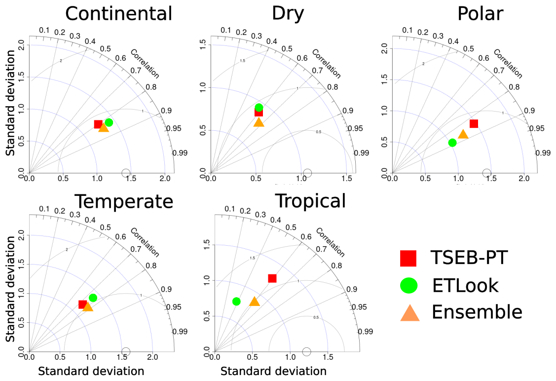
Figure C2Taylor plots on the performance of the dekadal ET from TSEB-PT, ETLook and Ensemble datasets. Sites grouped per climate region (Köppen climate classification system). For number of sites in each group see Fig. 6. Azimuthal angle represents the Pearson r, radial distance from the origin is the standard deviation (mm d−1). Circle marker at the horizontal axis represents perfect model performance, markers closer to this point indicate better model performance. Radial distance from this point is equivalent to centered RMSE (contour values shown in mm d−1).
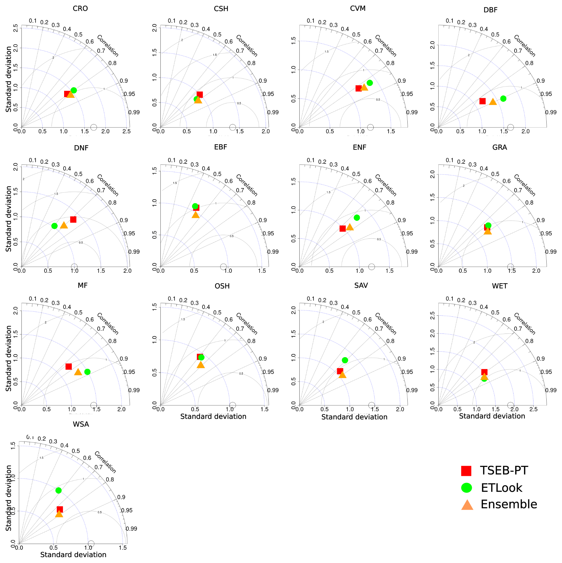
Figure C3Taylor plots on the performance of the dekadal ET from TSEB-PT, ETLook and Ensemble datasets. Sites grouped per Plant Functional Type. For number of sites in each group see Fig. 6. Azimuthal angle represents the Pearson r, radial distance from the origin is the standard deviation (mm d−1). Circle marker at the horizontal axis represents perfect model performance, markers closer to this point indicate better model performance. Radial distance from this point is equivalent to centered RMSE (contour values shown in mm d−1).
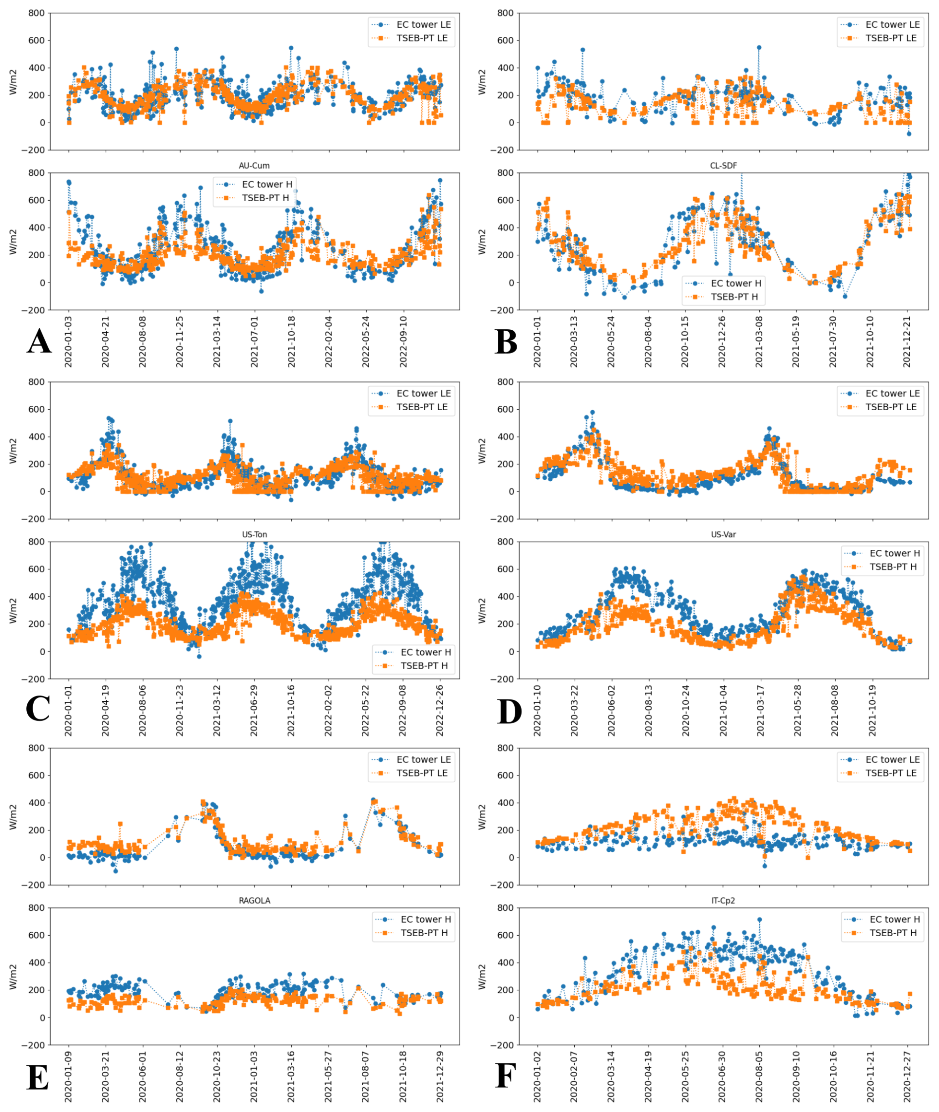
Figure C4Timeseries plots of LE (top panels) and H (bottom panels) (W m−2) as measured at the eddy covariance stations (blue) and as modelled by TSEB-PT (orange) at satellite overpass time in AU-Cum (EBF), CL-SDF (EBF), US-Ton (WSA), US-Var (GRA), Ragola (GRA) and IT-Cp2 (EBF) sites.
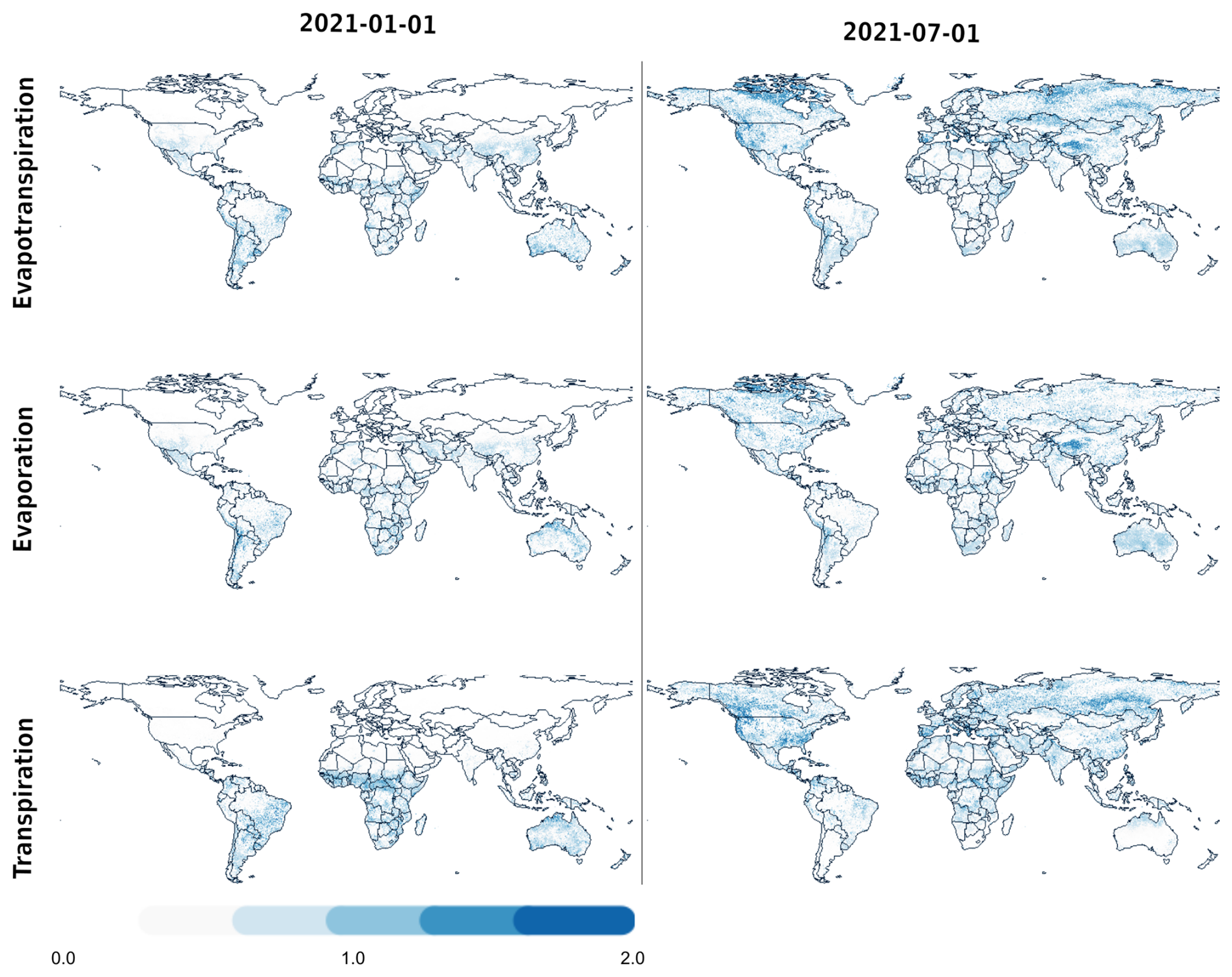
Figure C5Absolute differences (mm d−1) between estimates of ET, E and T of the ETLook and TSEB-pT models on the first dekad of January and July 2021.
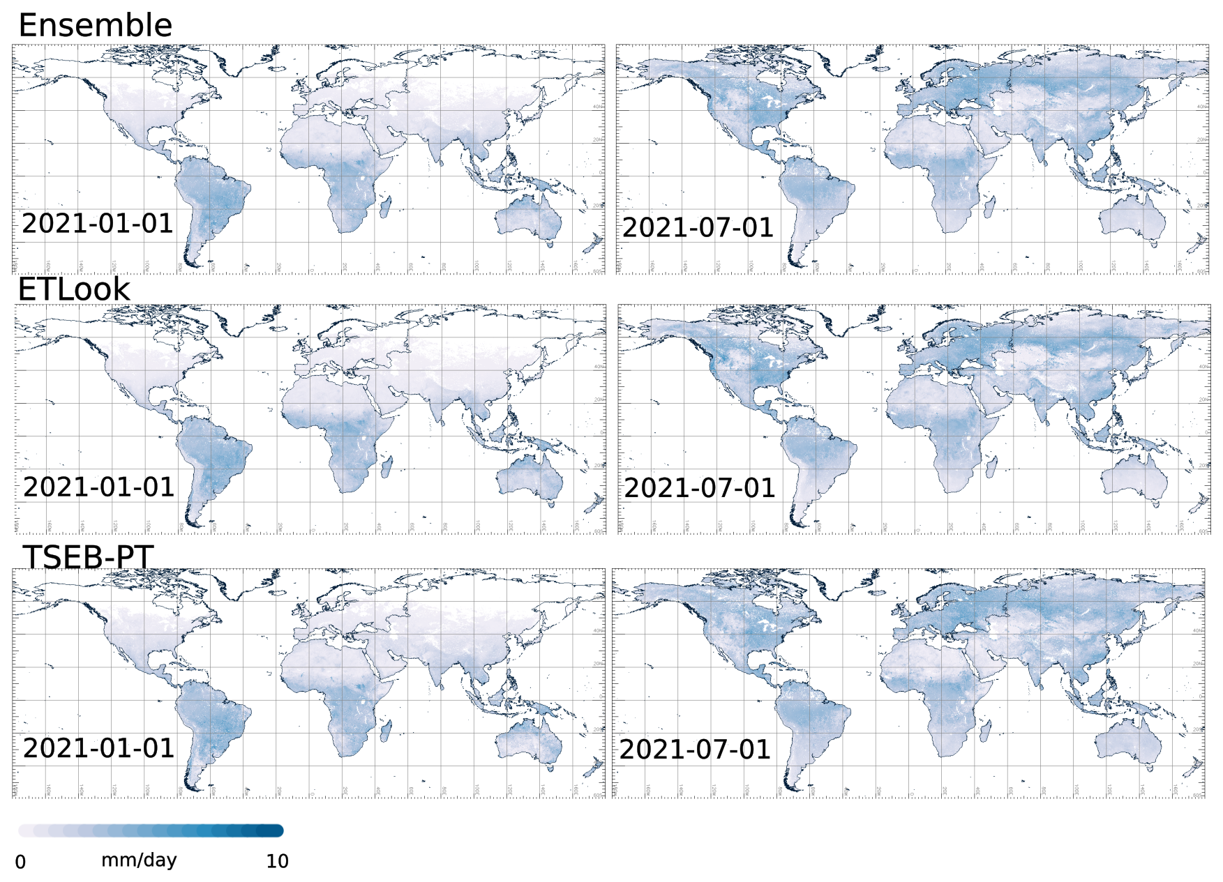
Figure C6Global maps of the Ensemble, ETLook and TSEB-PT ET estimates for norther hemisphere winter (left panels – first dekad of January 2021) and northern hemisphere summer (right panels – first dekad of July 2021).
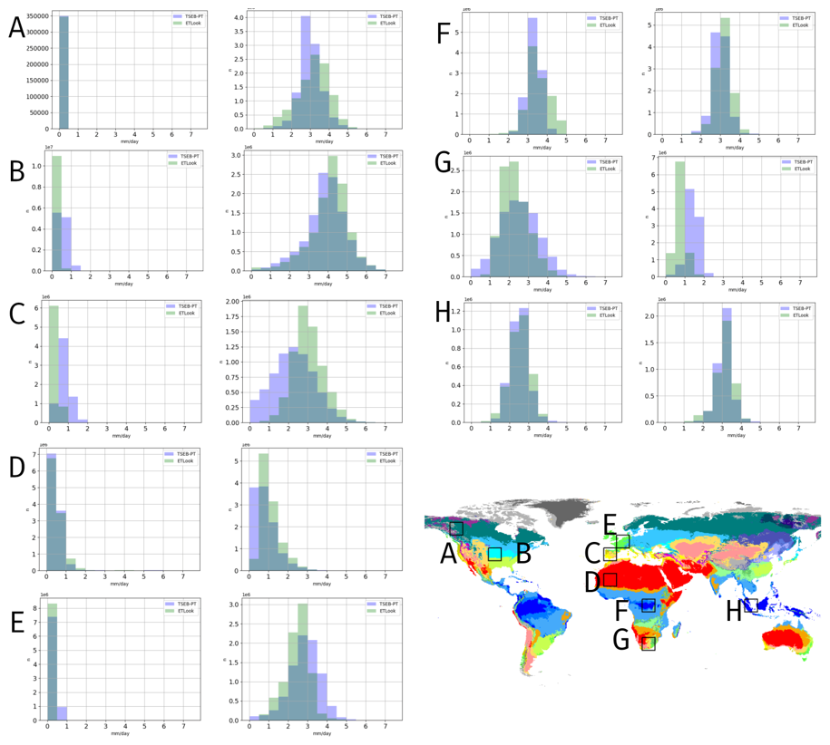
Figure C7Histograms of TSEB-PT (blue) and ETLook (green) dekadal ET in first dekads of January (left panels) and of July (right panels) 2021 across 10° lat/lon tiles located in different climate regions according to the Köppen classification system. Climate types per region: A – Dfc; B – Dfa; C – mosaic of Csa, BSk, Csb, Cfb; D – BWh; E – Cfb; F – Af; G – mosaic of BWh, BSk, Cwb, Cfb; H – Af.
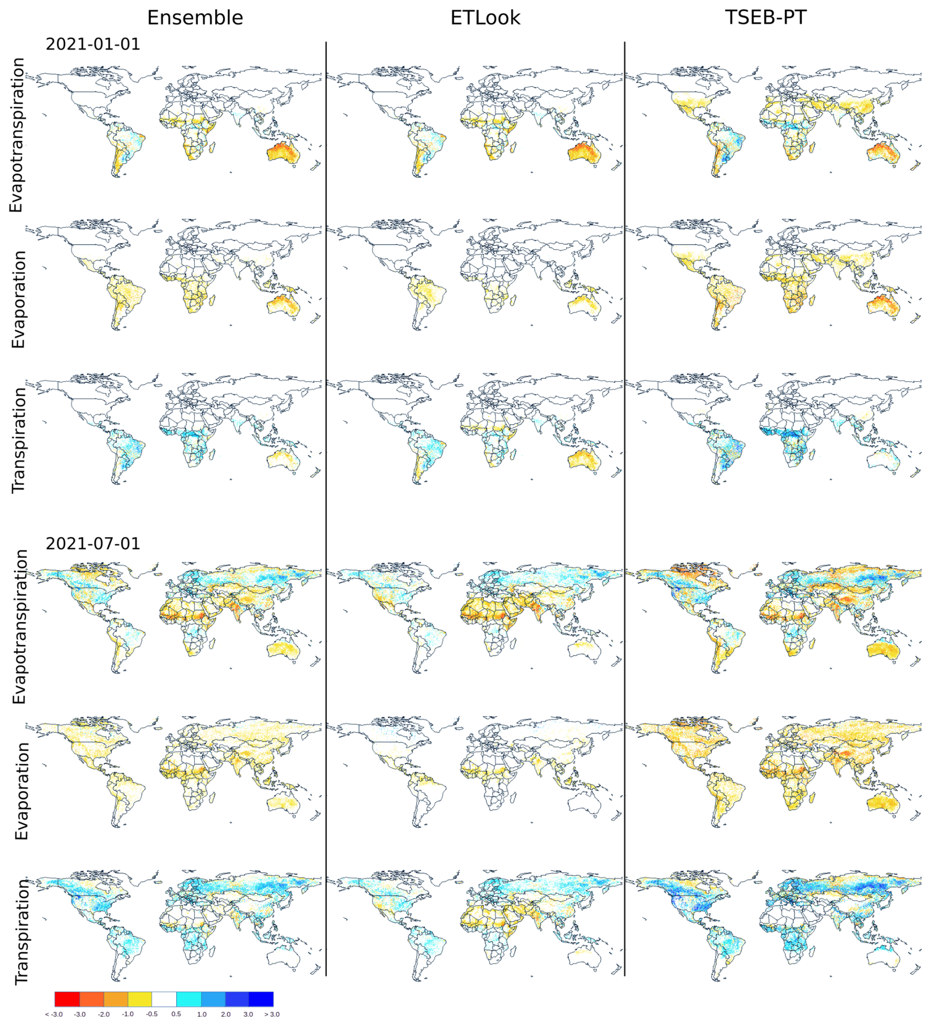
Figure C8Differences (WaPOR − CLMS: mm d−1) between estimates of ET, E and T of the two products on the first dekad of January and July 2021.
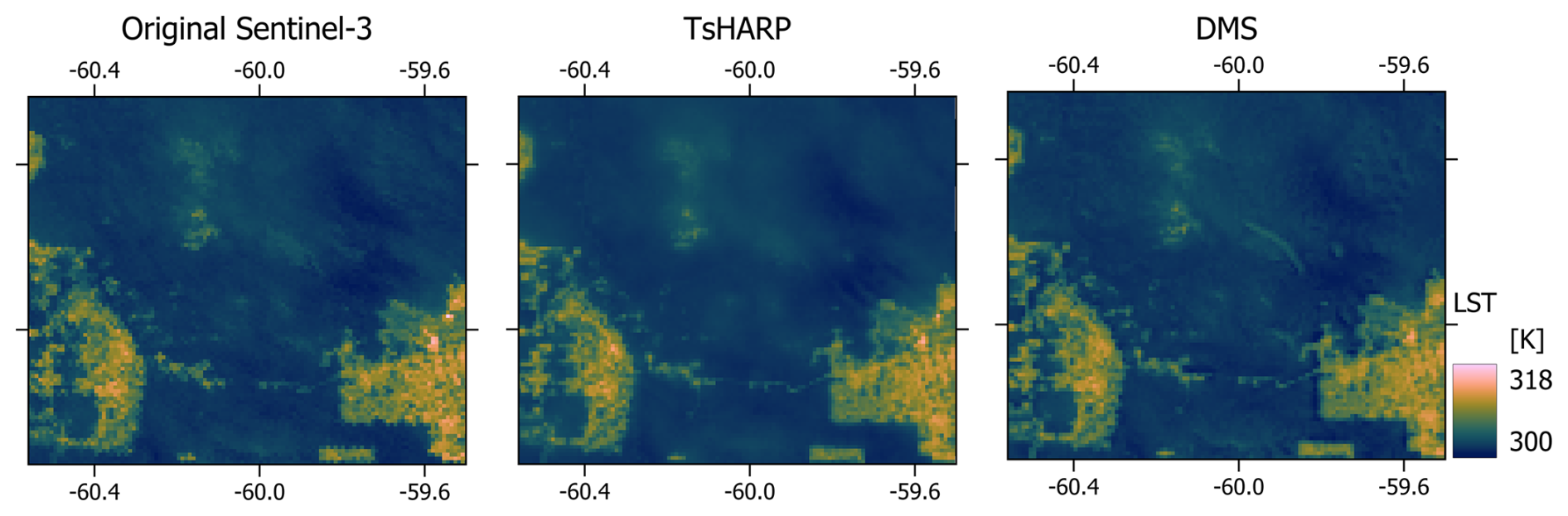
Figure C9Example from Amazon rainforest (forested and cleared areas) of original 1 km resolution Sentinel-3 LST and Sentinel-1 LST resampled to 3 km and then sharpened back to 1 km using TsHARP and DMS (see Sect. 4.3.2 for details).
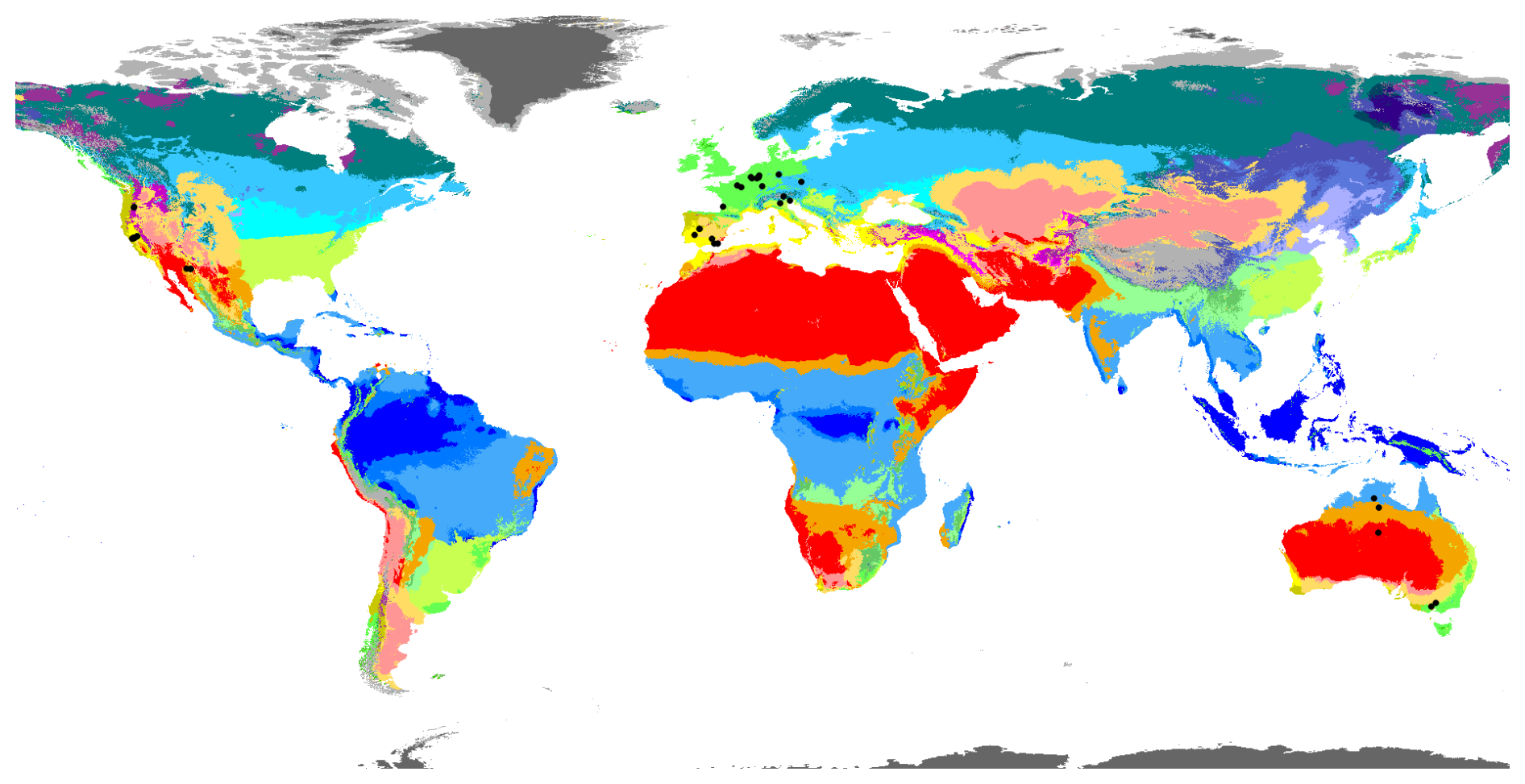
Figure C10Location of sites used to evaluate CAMS meteorological data (Sect. 4.3.3). Background map shows Köppen climate classification.
Table C2Accuracy statistics for thermal sharpening: coefficient of determination (r2), Root Mean Square Error (RMSE), Mean Absolute Error (MAE), bias (modelled minus observed) and slope of the linear regression line between modelled and observed values. Model configurations are described in Sect. 2.2.4.
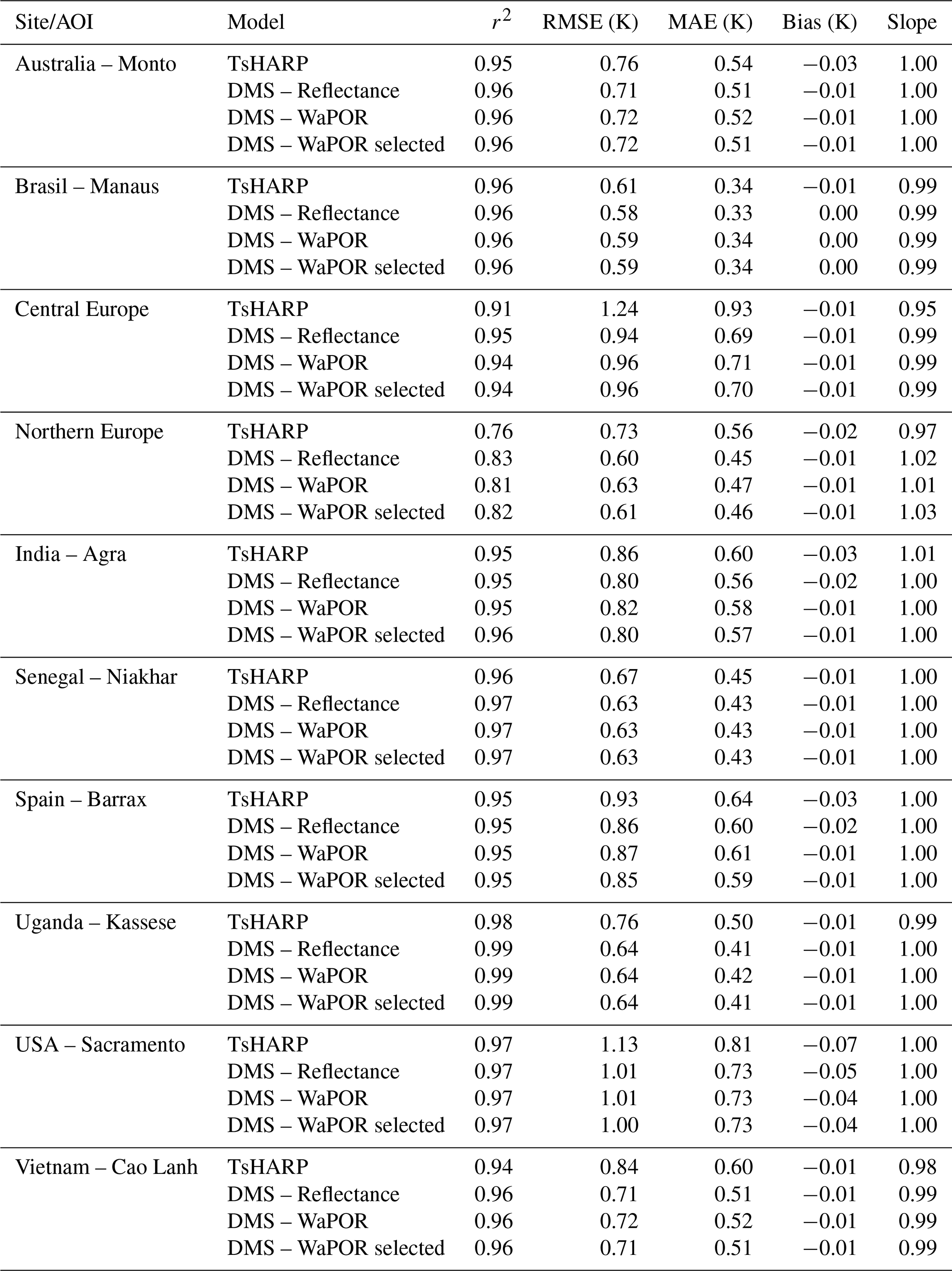
The biophysical processor based on PROSPECTD+4SAIL described in Sect. 2.2.2 is available at https://github.com/hectornieto/pyPro4Sail (last access: 27 August 2026) with the specific version used in this study being https://github.com/hectornieto/pypro4sail/releases/tag/v1.2 (last access: 27 August 2026; https://doi.org/10.5281/zenodo.15094926, Nieto, 2025).
The Data Mining Sharpener used to sharpen LST described in Sect. 2.2.4 is available at https://github.com/radosuav/pyDMS (last access: 27 August 2026) with the specific version used in this study being https://github.com/radosuav/pyDMS/releases/tag/v1.2 (last access: 1 September 2026; https://doi.org/10.5281/zenodo.22237789, Guzinski et al., 2026).
The code used to access and topographically correct meteorological forcings described in Sect. 2.2.5 is available at https://github.com/hectornieto/meteo_utils/ (last access: 27 August 2026) with the specific version used in this study being https://github.com/hectornieto/meteo_utils/releases/tag/v2.1.1 (last access: 27 August 2026; https://doi.org/10.5281/zenodo.15095543, Nieto et al., 2025b).
The implementation of TSEB-PT model described in Sect. 2.1.1 is available at https://github.com/hectornieto/pyTSEB (last access: 27 August 2026) the specific version used in this study being https://github.com/hectornieto/pyTSEB/releases/tag/v2.3 (last access: 27 August 2026; https://doi.org/10.5281/zenodo.15094917, Nieto et al., 2025a).
The implementation of ETLook model described in Sect. 2.1.2 is available at https://github.com/un-fao/fao-wetl-pywapor (Coerver and FAO WaPOR Team, 2026) with the specific version used in this study being https://github.com/DHI-GRAS/pywapor/releases/tag/v1.0-clms_eta (Guzinski and DHI, 2026).
The near-real-time ETa data produced by Copernicus Land Monitoring Service (https://doi.org/10.2909/861003ed-2082-41ea-9eb5-b068ca63b168, Copernicus Land Monitoring Service, 2025e) can be accessed from Copernicus Data Space Ecosystem (https://dataspace.copernicus.eu/, last access: 27 August 2026).
RG contributed to the input forcing analysis, integration of the processing chain and data production as well as the pyDMS code. HN contributed to the input forcing analysis and pyTSEB, pyPro4SAIL and meteo_utils code. JMB, FGM and JDP contributed to in-situ and WaPOR data collection and model validation. WG contributed to evaluation of LST sharpening methods. RL contributed to the funding acquisition and coordinated the presented work.
The contact author has declared that none of the authors has any competing interests.
Publisher's note: Copernicus Publications remains neutral with regard to jurisdictional claims made in the text, published maps, institutional affiliations, or any other geographical representation in this paper. The authors bear the ultimate responsibility for providing appropriate place names. Views expressed in the text are those of the authors and do not necessarily reflect the views of the publisher.
We would like to acknowledge the helpful interactions with Livia Peiser, Jippe Hoogeveen and Bert Coerver from FAO WaPOR team and their support with access to the WaPOR/ETLook code. We would also like to thank Dominique De Munck from VITO for great help with data production.
This work utilized data from the Integrated Carbon Observation System (ICOS – https://www.icos-cp.eu/, last access: 27 August 2026), the OzFlux network (https://www.ozflux.org.au/, last access: 27 August 2026) which is supported by the Australian Terrestrial Ecosystem Research Network (TERN – http://www.tern.org.au, last access: 27 August 2026), the AmeriFlux network (https://ameriflux.lbl.gov/, last access: 27 August 2026; funding for the AmeriFlux data portal was provided by the U.S. Department of Energy Office of Science), the European Fluxes Database Cluster (EFDC – https://www.europe-fluxdata.eu/), l'observatoire AMMA-CATCH (Analyse Multidisciplinaire de la Mousson Africaine – Couplage de l'Atmosphère Tropicale et du Cycle Hydrologique – https://www.amma-catch.org/, last access: 27 August 2026) and the AsiaFlux network (https://asiaflux.net/index.php, last access: 27 August 2026).
The presented work was funded by Specific Contract no. 4 of the implementing framework contract no. 945120 – IPR – 2023 with the European Union represented by European Commission, Directorate-General Joint Research Centre.
This paper was edited by Adriaan J. (Ryan) Teuling and Bob Su and reviewed by Xuelong Chen, Prajwal Khanal, Annemarie Klaasse, Bich Ngoc Tran, and one anonymous referee.
Abbasi, B., Qin, Z., Du, W., Li, S., Fan, J., and Zhao, S.: Effects of Cloud on Land Surface Temperature (LST) Change in Thermal Infrared Remote Sensing Images: a Case Study of Landsat 8 Data, in: IGARSS 2020 – 2020 IEEE International Geoscience and Remote Sensing Symposium, IEEE, Waikoloa, HI, USA, ISBN 978-1-7281-6374-1, 5430–5433, https://doi.org/10.1109/IGARSS39084.2020.9324415, 2020. a
Agam, N., Kustas, W. P., Anderson, M. C., Li, F., and Neale, C. M. U.: A vegetation index based technique for spatial sharpening of thermal imagery, Remote Sens. Environ., 107, 545–558, https://doi.org/10.1016/j.rse.2006.10.006, 2007. a, b
Alfieri, J. G., Kustas, W. P., Nieto, H., Prueger, J. H., Hipps, L. E., McKee, L. G., Gao, F., and Los, S.: Influence of wind direction on the surface roughness of vineyards, Irrigation Sci., 37, 359–373, https://doi.org/10.1007/s00271-018-0610-z, 2019. a, b
Allen, R. G. (Ed.): Crop evapotranspiration: guidelines for computing crop water requirements, no. 56 in FAO irrigation and drainage paper, Food and Agriculture Organization of the United Nations, Rome, repr. edition, ISBN 978-92-5-104219-9, 1998. a, b, c
AMMA-CATCH: AMMA-CATCH: a hydrological, meteorological and ecological observatory on West Africa, IRD, CNRS-INSU, OSUG, OMP, OREME, https://doi.org/10.17178/AMMA-CATCH.all, 1990. a
Anderson, M. C., Hain, C., Wardlow, B., Pimstein, A., Mecikalski, J. R., and Kustas, W. P.: Evaluation of Drought Indices Based on Thermal Remote Sensing of Evapotranspiration over the Continental United States, J. Climate, 24, 2025–2044, https://doi.org/10.1175/2010JCLI3812.1, 2011. a
Anderson, M. C., Kustas, W. P., Norman, J. M., Diak, G. T., Hain, C. R., Gao, F., Yang, Y., Knipper, K. R., Xue, J., Yang, Y., Crow, W. T., Holmes, T. R., Nieto, H., Guzinski, R., Otkin, J. A., Mecikalski, J. R., Cammalleri, C., Torres-Rua, A. T., Zhan, X., Fang, L., Colaizzi, P. D., and Agam, N.: A brief history of the thermal IR-based Two-Source Energy Balance (TSEB) model – diagnosing evapotranspiration from plant to global scales, Agr. Forest Meteorol., 350, 109951, https://doi.org/10.1016/j.agrformet.2024.109951, 2024. a, b
Baker, J. and Griffis, T.: AmeriFlux FLUXNET-1F US-Ro5 Rosemount I18-South, v1.3-r1, AmeriFlux AMP [data set], https://doi.org/10.17190/AMF/1818371, 2025a. a
Baker, J. and Griffis, T.: AmeriFlux FLUXNET-1F US-Ro6 Rosemount I18-North, v1.3-r1, AmeriFlux AMP [data set], https://doi.org/10.17190/AMF/1881590, 2025b. a
Baker, J. and Griffis, T.: AmeriFlux FLUXNET-1F US-Ro4 Rosemount Prairie, v1.3-r1, AmeriFlux AMP [data set], https://doi.org/10.17190/AMF/1881589, 2026. a
Barrios, J. M., Arboleda, A., Dutra, E., Trigo, I., and Gellens‐Meulenberghs, F.: Evapotranspiration and surface energy fluxes across Europe, Africa and Eastern South America throughout the operational life of the Meteosat second generation satellite, Geosci. Data J., gdj3.235, https://doi.org/10.1002/gdj3.235, 2024. a
Barrios, J. M., de Pue, J., and Meulenberghs, F.: Validation Report – Evapotranspiration and Heat Flux 300 m, Tech. Rep. I1.00, Copernicus Land Monitoring Service, https://land.copernicus.eu/en/technical-library/validation-report-evapotranspiration-version-1.0/@@download/file (last access: 27 August 2026), 2025. a
Bastiaanssen, W. G. M., Cheema, M. J. M., Immerzeel, W. W., Miltenburg, I. J., and Pelgrum, H.: Surface energy balance and actual evapotranspiration of the transboundary Indus Basin estimated from satellite measurements and the ETLook model, Water Resour. Res., 48, https://doi.org/10.1029/2011WR010482, 2012. a, b, c, d
Biraus, S., Fischer, M., Chan, S., and Torn, M.: AmeriFlux FLUXNET-1F US-ARM ARM Southern Great Plains site- Lamont, v1.3-r1, AmeriFlux AMP [data set], https://doi.org/10.17190/AMF/1854366, 2026. a
Blatchford, M. L., Mannaerts, C. M., Njuki, S. M., Nouri, H., Zeng, Y., Pelgrum, H., Wonink, S., and Karimi, P.: Evaluation of WaPOR V2 evapotranspiration products across Africa, Hydrol. Process., 34, 3200–3221, https://doi.org/10.1002/hyp.13791, 2020. a, b
Bojinski, S., Verstraete, M., Peterson, T. C., Richter, C., Simmons, A., and Zemp, M.: The Concept of Essential Climate Variables in Support of Climate Research, Applications, and Policy, B. Am. Meteorol. Soc., 95, 1431–1443, https://doi.org/10.1175/BAMS-D-13-00047.1, 2014. a
Boone, A., Bellvert, J., Best, M., Brooke, J. K., Canut-Rocafort, G., Cuxart, J., Hartogensis, O., Moigne, P. L., Miró, J. R., Polcher, J., Price, J., Seguí, P. Q., Bech, J., Bezombes, Y., Branch, O., Cristóbal, J., Dassas, K., Fanise, P., Gibert, F., Goulas, Y., Groh, J., Hanus, J., Hmimina, G., Jarlan, L., Kim, E., Dantec, V. L., Page, M. L., Lohou, F., Lothon, M., Mangan, M. R., Martí, B., Martínez-Villagrasa, D., McGregor, J., Kerr-Munslow, A., Ouaadi, N., Philibert, A., Quiros-Vargas, J., Rascher, U., Siegmann, B., Udina, M., Vial, A., Wrenger, B., Wulfmeyer, V., and Zribi, M.: The Land Surface Interactions with the Atmosphere over the Iberian Semi-Arid Environment (LIAISE) field campaign, Journal of the European Meteorological Society, 2, 100007, https://doi.org/10.1016/j.jemets.2025.100007, 2025. a
Bulgin, C., Sembhi, H., Ghent, D., Remedios, J., and Merchant, C.: Cloud-clearing techniques over land for land-surface temperature retrieval from the Advanced Along-Track Scanning Radiometer, Int. J. Remote Sens., 35, 3594–3615, https://doi.org/10.1080/01431161.2014.907941, 2014. a
Burchard-Levine, V., Nieto, H., Riaño, D., Migliavacca, M., El-Madany, T. S., Perez-Priego, O., Carrara, A., and Martín, M. P.: Seasonal Adaptation of the Thermal-Based Two-Source Energy Balance Model for Estimating Evapotranspiration in a Semiarid Tree-Grass Ecosystem, Remote Sens., 12, 904, https://doi.org/10.3390/rs12060904, 2020. a, b
Camillo, P. J. and Gurney, R. J.: A Resistance Parameter For Bare-Soil Evaporation Models, Soil Sci., 141, 95–105, https://doi.org/10.1097/00010694-198602000-00001, 1986. a
Cammalleri, C., Anderson, M. C., and Kustas, W. P.: Upscaling of evapotranspiration fluxes from instantaneous to daytime scales for thermal remote sensing applications, Hydrol. Earth Syst. Sci., 18, 1885–1894, https://doi.org/10.5194/hess-18-1885-2014, 2014. a
Campbell, G.: Derivation of an angle density function for canopies with ellipsoidal leaf angle distributions, Agr. Forest Meteorol., 49, 173–176, https://doi.org/10.1016/0168-1923(90)90030-A, 1990. a, b, c, d, e
Campbell, G. S. and Norman, J. M.: The Light Environment of Plant Canopies, in: An Introduction to Environmental Biophysics, Springer New York, New York, NY, ISBN 978-0-387-94937-6, 247–278, https://doi.org/10.1007/978-1-4612-1626-1_15, 1998. a, b, c
Christen, A. and Knox, S.: AmeriFlux FLUXNET-1F CA-DBB Delta Burns Bog, v1.3-r1, AmeriFlux AMP [data set], https://doi.org/10.17190/AMF/1881565, 2025. a
Chu, H., Christianson, D. S., Cheah, Y.-W., Pastorello, G., O'Brien, F., Geden, J., Ngo, S.-T., Hollowgrass, R., Leibowitz, K., Beekwilder, N. F., Sandesh, M., Dengel, S., Chan, S. W., Santos, A., Delwiche, K., Yi, K., Buechner, C., Baldocchi, D., Papale, D., Keenan, T. F., Biraud, S. C., Agarwal, D. A., and Torn, M. S.: AmeriFlux BASE data pipeline to support network growth and data sharing, Scientific Data, 10, 614, https://doi.org/10.1038/s41597-023-02531-2, 2023. a
Chukalla, A. D., Mul, M. L., van der Zaag, P., van Halsema, G., Mubaya, E., Muchanga, E., den Besten, N., and Karimi, P.: A framework for irrigation performance assessment using WaPOR data: the case of a sugarcane estate in Mozambique, Hydrol. Earth Syst. Sci., 26, 2759–2778, https://doi.org/10.5194/hess-26-2759-2022, 2022. a
Coerver, B. and FAO WaPOR Team: pyWaPOR, GitHub [code], https://github.com/un-fao/fao-wetl-pywapor, last access: 1 September 2026. a
Cogill, L. S., Toucher, M., Wolski, P., Esler, K. J., and Rebelo, A. J.: Evaluating the performance of satellite-derived evapotranspiration products across varying bioclimates in South Africa, Remote Sensing Applications: Society and Environment, 38, 101612, https://doi.org/10.1016/j.rsase.2025.101612, 2025. a
Comini De Andrade, B., Laipelt, L., Fleischmann, A., Huntington, J., Morton, C., Melton, F., Erickson, T., Roberti, D. R., De Arruda Souza, V., Biudes, M., Gomes Machado, N., Antonio Costa Dos Santos, C., Cosio, E. G., and Ruhoff, A.: geeSEBAL-MODIS: Continental-scale evapotranspiration based on the surface energy balance for South America, ISPRS J. Photogramm., 207, 141–163, https://doi.org/10.1016/j.isprsjprs.2023.12.001, 2024. a
Copernicus Land Monitoring Service: Land Cover 2015-2019 (raster 100 m), global, annual – version 3, Copernicus Data Space Ecosystem (CDSE), https://doi.org/10.2909/C6377C6E-76CC-4D03-8330-628A03693042, 2015. a
Copernicus Land Monitoring Service: Fraction of Absorbed Photosynthetically Active Radiation 2014-present (raster 300 m), global, 10-daily – version 1, Copernicus Data Space Ecosystem (CDSE), https://doi.org/10.2909/5A38461B-3EF7-4F97-A933-4C9F51A0EDA5, 2017a. a
Copernicus Land Monitoring Service: Leaf Area Index 2014-present (raster 300 m), global, 10-daily – version 1, Copernicus Data Space Ecosystem (CDSE), https://doi.org/10.2909/219FDC9F-616B-444B-A495-198F527B4722, 2017b. a
Copernicus Land Monitoring Service: Product User Manual – Leaf Area Index (LAI), Fraction of Absorbed Photosynthetically Active Radiation (FAPAR), Fraction of green Vegetation Cover (FCover), Collection 300 m, Version 1.1, Tech. rep., Copernicus Land Monitoring Service, https://land.copernicus.eu/en/technical-library/product-user-manual-leaf-area-index-333-m-version-1-1 (last access: 5 August 2025), 2022. a
Copernicus Land Monitoring Service: Validation Report – LAI, FAPAR, FCOVER from Sentinel-3/OLCI, version 2.1, Tech. rep., Copernicus Land Monitoring Service, https://land.copernicus.eu/en/technical-library/quality-assessment-report-leaf-area-index-300m-version-1-1-annex-update-2023/@@download/file (last access: 4 August 2025), 2025a. a
Copernicus Land Monitoring Service: Sentinel-3 Top-Of-Canopy Reflectance 2018-present (raster 300 m), global, daily – version 2, Copernicus Data Space Ecosystem (CDSE), https://doi.org/10.2909/B4149B9B-F020-42EA-9159-9C437CE4C15B, 2025b. a
Copernicus Land Monitoring Service: Validation Report – Surface Reflectance, Version 2.3, Tech. rep., Copernicus Land Monitoring Service, https://land.copernicus.eu/en/technical-library/validation-report-surface-reflectance-300m-version-2-3/@@download/file (last access: 4 August 2025), 2025c. a
Copernicus Land Monitoring Service: Product User Manual – Sentinel-3 OLCI and SLSTR Surface Reflectance, Version 2.3, Tech. rep., Copernicus Land Monitoring Service, https://land.copernicus.eu/en/technical-library/product-user-manual-surface-reflectance-300m-version-2.3/@@download/file (last access: 4 August 2025), 2025d. a
Copernicus Land Monitoring Service: Evapotranspiration 2025–present (raster 300 m), global, 10-daily – version 1, Copernicus Land Monitoring Service [data set], https://doi.org/10.2909/861003ed-2082-41ea-9eb5-b068ca63b168, 2025e. a
Delogu, E., Olioso, A., Alliès, A., Demarty, J., and Boulet, G.: Evaluation of Multiple Methods for the Production of Continuous Evapotranspiration Estimates from TIR Remote Sensing, Remote Sens., 13, 1086, https://doi.org/10.3390/rs13061086, 2021. a
Djamai, N., Fernandes, R., Weiss, M., McNairn, H., and Goïta, K.: Validation of the Sentinel Simplified Level 2 Product Prototype Processor (SL2P) for mapping cropland biophysical variables using Sentinel-2/MSI and Landsat-8/OLI data, Remote Sens. Environ., 225, 416–430, https://doi.org/10.1016/j.rse.2019.03.020, 2019. a
Donlon, C., Berruti, B., Buongiorno, A., Ferreira, M. H., Féménias, P., Frerick, J., Goryl, P., Klein, U., Laur, H., Mavrocordatos, C., Nieke, J., Rebhan, H., Seitz, B., Stroede, J., and Sciarra, R.: The Global Monitoring for Environment and Security (GMES) Sentinel-3 mission, Remote Sens. Environ., 120, 37–57, https://doi.org/10.1016/j.rse.2011.07.024, 2012. a, b
Eichelmann, E., Shortt, R., Knox, S., Rey Sanchez, C., Valach, A., Sturtevant, C., Szutu, D., Verfaillie, J., and Baldocchi, D.: AmeriFlux FLUXNET-1F US-Tw4 Twitchell East End Wetland, v1.3-r1, AmeriFlux AMP [data set], https://doi.org/10.17190/AMF/2204881, 2026. a
Eilers, P. H. C.: A Perfect Smoother, Anal. Chem., 75, 3631–3636, https://doi.org/10.1021/ac034173t, 2003. a
European Space Agency and Airbus: Copernicus DEM, European Space Agency, https://doi.org/10.5270/ESA-c5d3d65, 2022. a, b
Euskirchen, E: AmeriFlux FLUXNET-1F US-BZF Bonanza Creek Rich Fen, v1.3-r1, AmeriFlux AMP [data set], https://doi.org/10.17190/AMF/1881570, 2026. a
Feret, J.-B., François, C., Asner, G. P., Gitelson, A. A., Martin, R. E., Bidel, L. P., Ustin, S. L., Le Maire, G., and Jacquemoud, S.: PROSPECT-4 and 5: Advances in the leaf optical properties model separating photosynthetic pigments, Remote Sens. Environ., 112, 3030–3043, https://doi.org/10.1016/j.rse.2008.02.012, 2008. a
Féret, J.-B., Gitelson, A., Noble, S., and Jacquemoud, S.: PROSPECT-D: Towards modeling leaf optical properties through a complete lifecycle, Remote Sens. Environ., 193, 204–215, https://doi.org/10.1016/j.rse.2017.03.004, 2017. a, b, c
Féret, J.-B., Berger, K., De Boissieu, F., and Malenovský, Z.: PROSPECT-PRO for estimating content of nitrogen-containing leaf proteins and other carbon-based constituents, Remote Sens. Environ., 252, 112173, https://doi.org/10.1016/j.rse.2020.112173, 2021. a
Fisher, J. B., Tu, K. P., and Baldocchi, D. D.: Global estimates of the land–atmosphere water flux based on monthly AVHRR and ISLSCP-II data, validated at 16 FLUXNET sites, Remote Sens. Environ., 112, 901–919, https://doi.org/10.1016/j.rse.2007.06.025, 2008. a, b
Flerchinger, G.: AmeriFlux FLUXNET-1F US-Rls RCEW Low Sagebrush, v1.3-r1, AmeriFlux AMP [data set], https://doi.org/10.17190/AMF/2229387, 2026. a
Foken, T., Aubinet, M., Finnigan, J. J., Leclerc, M. Y., Mauder, M., and Paw U, K. T.: Results Of A Panel Discussion About The Energy Balance Closure Correction For Trace Gases, B. Am. Meteorol. Soc., 92, ES13–ES18, https://doi.org/10.1175/2011BAMS3130.1, 2011. a
Forsythe, J. D., Kline, M. A., and O'Halloran, T. L.: AmeriFlux FLUXNET-1F US-HB3 Hobcaw Barony Longleaf Pine Restoration, v1.3-r1, AmeriFlux AMP [data set], https://doi.org/10.17190/AMF/2229378, 2026. a
FRAME Consortium: WaPOR methodology, version 3, https://github.com/un-fao/wapor-et-look/wiki (last access: 27 August 2026), 2024. a, b, c, d
Galle, S., Grippa, M., Peugeot, C., Moussa, I. B., Cappelaere, B., Demarty, J., Mougin, E., Panthou, G., Adjomayi, P., Agbossou, E., Ba, A., Boucher, M., Cohard, J.-M., Descloitres, M., Descroix, L., Diawara, M., Dossou, M., Favreau, G., Gangneron, F., Gosset, M., Hector, B., Hiernaux, P., Issoufou, B.-A., Kergoat, L., Lawin, E., Lebel, T., Legchenko, A., Abdou, M. M., Malam-Issa, O., Mamadou, O., Nazoumou, Y., Pellarin, T., Quantin, G., Sambou, B., Seghieri, J., Séguis, L., Vandervaere, J.-P., Vischel, T., Vouillamoz, J.-M., Zannou, A., Afouda, S., Alhassane, A., Arjounin, M., Barral, H., Biron, R., Cazenave, F., Chaffard, V., Chazarin, J.-P., Guyard, H., Koné, A., Mainassara, I., Mamane, A., Oi, M., Ouani, T., Soumaguel, N., Wubda, M., Ago, E., Alle, I., Allies, A., Arpin-Pont, F., Awessou, B., Cassé, C., Charvet, G., Dardel, C., Depeyre, A., Diallo, F., Do, T., Fatras, C., Frappart, F., Gal, L., Gascon, T., Gibon, F., Guiro, I., Ingatan, A., Kempf, J., Kotchoni, D., Lawson, F., Leauthaud, C., Louvet, S., Mason, E., Nguyen, C., Perrimond, B., Pierre, C., Richard, A., Robert, E., Román-Cascón, C., Velluet, C., and Wilcox, C.: AMMA-CATCH, a Critical Zone Observatory in West Africa Monitoring a Region in Transition, Vadose Zone J., 17, 180062, https://doi.org/10.2136/vzj2018.03.0062, 2018. a
Gao, F., Masek, a. J., Schwaller, M., and Hall, F.: On the blending of the Landsat and MODIS surface reflectance: predicting daily Landsat surface reflectance, IEEE T. Geosci. Remote, 44, 2207–2218, https://doi.org/10.1109/TGRS.2006.872081, 2006. a
Gao, F., Kustas, W., and Anderson, M.: A Data Mining Approach for Sharpening Thermal Satellite Imagery over Land, Remote Sens., 4, 3287, https://doi.org/10.3390/rs4113287, 2012. a, b
Garratt, J. and Hicks, B.: Momentum, heat and water vapour transfer to and from natural and artificial surfaces, Q. J. Roy. Meteor. Soc., 99, 680–687, https://doi.org/10.1002/qj.49709942209, 1973. a
Gómez-Candón, D., Bellvert, J., and Royo, C.: Performance of the Two-Source Energy Balance (TSEB) Model as a Tool for Monitoring the Response of Durum Wheat to Drought by High-Throughput Field Phenotyping, Front. Plant Sci., 12, 658357, https://doi.org/10.3389/fpls.2021.658357, 2021. a
Gueymard, C. A.: REST2: High-performance solar radiation model for cloudless-sky irradiance, illuminance, and photosynthetically active radiation – Validation with a benchmark dataset, Sol. Energy, 82, 272–285, https://doi.org/10.1016/j.solener.2007.04.008, 2008. a
Guzinski, R. and DHI: CLMS ETA: Copernicus Adaptation of pyWaPOR, v1.0-clms_eta, Fork of FAO pyWaPOR, GitHub [code], https://github.com/DHI-GRAS/pywapor/releases/tag/v1.0-clms_eta, last access: 1 September 2026. a
Guzinski, R. and Nieto, H.: Evaluating the feasibility of using Sentinel-2 and Sentinel-3 satellites for high-resolution evapotranspiration estimations, Remote Sens. Environ., 221, 157–172, https://doi.org/10.1016/j.rse.2018.11.019, 2019. a
Guzinski, R., Nieto, H., Sandholt, I., and Karamitilios, G.: Modelling High-Resolution Actual Evapotranspiration through Sentinel-2 and Sentinel-3 Data Fusion, Remote Sens., 12, 1433, https://doi.org/10.3390/rs12091433, 2020. a, b, c, d, e, f, g
Guzinski, R., Nieto, H., Sanchez, J. M., Lopez-Urrea, R., Boujnah, D. M., and Boulet, G.: Utility of Copernicus-Based Inputs for Actual Evapotranspiration Modeling in Support of Sustainable Water Use in Agriculture, IEEE J. Sel. Top. Appl., 14, 11466–11484, https://doi.org/10.1109/JSTARS.2021.3122573, 2021. a, b, c, d, e, f, g, h
Guzinski, R., Nieto, H., Ramo Sánchez, R., Sánchez, J. M., Jomaa, I., Zitouna-Chebbi, R., Roupsard, O., and López-Urrea, R.: Improving field-scale crop actual evapotranspiration monitoring with Sentinel-3, Sentinel-2, and Landsat data fusion, Int. J. Appl. Earth Obs., 125, 103587, https://doi.org/10.1016/j.jag.2023.103587, 2023. a, b, c, d
Guzinski, R., Lund Larsen, M., and Nieto, H.: radosuav/pyDMS: v1.3_zenodo (Version v1.3_zenodo), Zenodo [code], https://doi.org/10.5281/zenodo.22237789, 2026. a
Hajirad, I., Mohammadi, S., and Dehghanisanij, H.: Determining the Critical Points of a Basin from the Point of View of Water Productivity and Water Consumption Using the WaPOR Database, in: The 7th International Electronic Conference on Water Sciences, p. 86, MDPI, https://doi.org/10.3390/ECWS-7-14322, 2023. a
Hanson, C., Still, C., and Law, B.: AmeriFlux FLUXNET-1F US-Me6 Metolius Young Pine Burn, v1.3-r1, AmeriFlux AMP [data set], https://doi.org/10.17190/AMF/2204871, 2026. a
He, S., Yang, Q., Zhang, L., Shi, Z., Wang, X., and Lv, B.: Consistency Assessment and Uncertainty Analysis of Spatial-temporal Characteristics of Evaporation Data in the Greater Mekong Subregion, J. Hydrometeorol., https://doi.org/10.1175/JHM-D-24-0014.1, 2025. a
Heiskanen, J., Brümmer, C., Buchmann, N., Calfapietra, C., Chen, H., Gielen, B., Gkritzalis, T., Hammer, S., Hartman, S., Herbst, M., Janssens, I. A., Jordan, A., Juurola, E., Karstens, U., Kasurinen, V., Kruijt, B., Lankreijer, H., Levin, I., Linderson, M.-L., Loustau, D., Merbold, L., Myhre, C. L., Papale, D., Pavelka, M., Pilegaard, K., Ramonet, M., Rebmann, C., Rinne, J., Rivier, L., Saltikoff, E., Sanders, R., Steinbacher, M., Steinhoff, T., Watson, A., Vermeulen, A. T., Vesala, T., Vítková, G., and Kutsch, W.: The Integrated Carbon Observation System in Europe, B. Am. Meteorol. Soc., 103, E855–E872, https://doi.org/10.1175/BAMS-D-19-0364.1, 2022. a
Hersbach, H., Bell, B., Berrisford, P., Hirahara, S., Horányi, A., Muñoz‐Sabater, J., Nicolas, J., Peubey, C., Radu, R., Schepers, D., Simmons, A., Soci, C., Abdalla, S., Abellan, X., Balsamo, G., Bechtold, P., Biavati, G., Bidlot, J., Bonavita, M., Chiara, G. D., Dahlgren, P., Dee, D., Diamantakis, M., Dragani, R., Flemming, J., Forbes, R., Fuentes, M., Geer, A., Haimberger, L., Healy, S., Hogan, R. J., Hólm, E., Janisková, M., Keeley, S., Laloyaux, P., Lopez, P., Lupu, C., Radnoti, G., Rosnay, P. D., Rozum, I., Vamborg, F., Villaume, S., and Thépaut, J.-N.: The ERA5 global reanalysis, Q. J. Roy. Meteor. Soc., 146, 1999–2049, https://doi.org/10.1002/qj.3803, 2020. a
Hosgood, B., Jacquemound, S., Andreeoli, G., Verdebout, J., Pedrini, A., and Schmuck, G.: Leaf Optical Properties Experiment Database (LOPEX93), Ecological Spectral Information System (EcoSIS), http://ecosis.org (last access: 2 September 2026), 1993. a
Huang, J., Sehgal, V., Alvarez, L. V., Brocca, L., Cai, S., Cheng, R., Cheng, X., Du, J., El Masri, B., Endsley, K. A., Fang, Y., Hu, J., Jampani, M., Kibria, M. G., Koren, G., Li, L., Liu, L., Mao, J., Moreno, H. A., Rigden, A., Shi, M., Shi, X., Wang, Y., Zhang, X., and Fisher, J. B.: Remotely Sensed High‐Resolution Soil Moisture and Evapotranspiration: Bridging the Gap Between Science and Society, Water Resour. Res., 61, e2024WR037929, https://doi.org/10.1029/2024WR037929, 2025. a
ICOS RI, Aalto, J., Aalto, P., Aaltonen, H., Aiguier, T., Akubia, J., Ala-Könni, J., Alivernini, A., Alonso, L., Aluome, C., Andersson, T., Arriga, N., Aurela, M., BRECHET, L., Baab, F., Back, J., Bagheri, S., Baltes, U., Baneschi, I., Barral, H., Barten, S., Bastos Campos, F., Baur, T., Bauters, M., Bazot, S., Beauclair, P., Becker, N., Behrens, N., Belelli Marchesini, L., Bergström, G., Bernhofer, C., Berveiller, D., Biermann, T., Bignotti, L., Biron, R., Bloor, J., Bodson, B., Boeckx, P., Boeske, L., Bogaerts, G., Bonal, D., Boon, G., Bornet, F., Bortoli, M., Boschetti, F., Bosio, I., Bresseleers, S., Brut, A., Brümmer, C., Buchmann, N., Bulonza, E., Burban, B., Burri, S., Buysse, P., Båth, A., Calandrelli, D., Calvet, J.-C., Canut-Rocafort, G., Carrara, A., Cash, J., Cavagna, M., Ceschia, E., Chabbi, A., Chan, T., Chebbi, W., Chebil, B., Chianucci, F., Chipeaux, C., Chopin, H., Christen, A., Chrysoulakis, N., Claverie, N., Cobbe, I., Cohard, J.-M., Colosse, D., Conte, A., Corsanici, R., Coulaud, C., Courtois, P., Coyle, M., Cremonese, E., Crill, P., Cuntz, M., Cuocolo, D., Czerný, R., Depuydt, J., Daelman, R., Darenová, E., Darsonville, O., De Ligne, A., De Meulder, T., De Simon, G., Decau, M.-L., Dejosez, S., Dell'Acqua, A., Delorme, J.-P., Delpierre, N., Demoulin, L., Denou, J.-L., Di Tommasi, P., Dienstbach, L., Dignam, R., Dolfus, D., Domec, J.-C., Douxfils, B., Drösler, M., Drüe, C., Dufrêne, E., Dumont, B., Durand, B., Dusek, J., Eberl, J., Eichelmann, U., Ekili, D., Engelmann, T., Esposito, A., Esser, O., Etienne, J.-C., Etzold, S., Eugster, W., Famulari, D., Fares, S., Faurès, A., Fauvel, Y., Feigenwinter, C., Feigenwinter, I., Feldmann, I., Ferraris, D., Filippa, G., Fincham, W., Finco, A., Fischer, M., Flechard, C., Folino, G., Foltýnová, L., Foret, J., Foulquier, A., François, B., Friborg, T., Galliot, J.-N., Galvagno, M., Garcia Quiros, I., Garrigou, C., Gastal, F., Geilfus, N.-X., Gerosa, G., Gessler, A., Gharun, M., Giamberini, M., Gianelle, D., Gibrin, H., Gimper, S., Gioli, B., Girardin, C., Goded, I., Graf, A., Granouillac, F., Grehan, E., Grenier, M., Grudd, H., Grünwald, T., Guillot, T., Guzman, R., Hamon, Y., Harvey, D., Hatakka, J., Haustein, A., Hautmann, D., Hehn, M., Heinesch, B., Helfter, C., Heliasz, M., Herbst, M., Hildebrandt, A., Holst, J., Holst, T., Holtmann, A., Hortnagl, L., Hug, C., Huguet, C., Häni, M., Ibrom, A., Ilardi, F., Jackowicz-Korczynski, M. A., Jacotot, A., Janssens, I., Jensen, R., Jocher, G., Joetzjer, E., Jones, M., Järvi, L., Kalalian, C., Kempf, J., Kempka, P., Keronen, P., Kettler, M., Kimbesa, F., Kivalov, S., Klatt, J., Klimo, P., Kljun, N., Klumpp, K., Kogxylakis, G., Kolari, P., Kolbe, S., Korkiakoski, M., Korrensalo, A., Kowalska, N., Kozii, N., Krejza, J., Kristoffersson, A., Kruijt, B., Kruszewski, A., Kulmala, L., Kumar, S., Kummer, S., Laakso, H., Lafont, S., Lange, H., Lange Rønn, E., Larmanou, E., Laurila, T., Leeson, S., Lefevre, L., Lehner, I., Lemaire, B., Leonard, J., Levula, J., Levy, P., Liechti, K., Liger, L., Lily, J.-B., Limousin, J.-M., Linderson, M.-L., Lindgren, K., Lo Cascio, M., Lodsgaard Justesen, M., Lofvenius, P., Lohila, A., Longdoz, B., Lootens, R., Loubet, B., Loustau, D., Lucarini, A., Lundin, E., López, R., López-Blanco, E., Magliulo, V., Mammarella, I., Manco, A., Manise, T., Marcolla, B., Marek, M. V., Marklund, P., Marloie, O., Marras, S., Martin, R., Martin Saint Paul, N., Marty, M., Martín, M. P., Marzuoli, R., Matilainen, T., Mattes, J., Matteucci, M., Mauder, M., Maurel, W., Mbifo, J., Meggio, F., Meier, F., Meier, P., Meire, A., Meis, J., Meissner, H., Mensah, C., Meyer, H., Michaud, L., Minerbi, S., Moderow, U., Molder, M., Montagnani, L., Moreno, G., Moretti, V., Morfin, A., Morra di Cella, U., Mullinger, N., Mäkelä, T., Männikkö, M., Männistö, E., Møller, F., Naiken, A., Naseer, M., Nemitz, E., Nezval, O., Nilsson, M., Norkko, J., Ocallaghan, F., Ojala, A., Orgun, A., Ottosson-Löfvenius, M., Ourcival, J.-M., Paasch, S., Paci, A., Pavelka, M., Pavot, L., Peichl, M., Peressotti, A., Perot-Guillaume, C., Perrot, C., Pihlatie, M., Pilegaard, K., Pilkottu, R., Piret, A., Pitacco, A., Plapp, T., Plebani, D., Politakos, K., Prasse, H., Provenzale, A., Pumpanen, J., Putzolu, S., Raco, B., Rainne, J., Rakos, N., Rebmann, C., Rebmann, C., Redepenning, D., Rinne, J., Rodeghiero, M., Roland, M., Rudd, D., Ryhti, K., Røjle Christensen, T., Sahoo, G., Salze, P., Schaarup Sørensen, J., Schindler, D., Schlaipfer, M., Schmidt, M., Schmidt, P., Schmitt Oehler, M., Schrader, F., Segers, J., Shivhalli Gopal, A., Sibret, T., Siivola, E., Simioni, G., Sirca, C., Smith, P., Snellen, H., Sorgi, T., Soudani, K., Spano, D., Spence, K., Spyridakis, N., Stagakis, S., Staník, K., Staudinger, M., Stecher, M., Stellner, S., Stutz, T., Suopajärvi, S., Sutter, F., Taipale, R., Tallec, T., Tenca, F., Tezza, L., Thimonier Rickenmann, A., Thyrion, T., Tomelleri, E., Trotsiuk, V., Trusina, J., Tuittila, E.-S., Tuovinen, J.-P., Tyssandier, J., Vagnoli, C., Valay, J.-G., Van Damme, F., Van Look, J., Vande Sompele, A., Vandome, E., Varjonen, S., Vendrame, N., Ventura, M., Verbeeck, H., Vesala, T., Vescovo, L., Vincent, G., Vincke, C., Vitale, L., Vivaldo, G., Voisin, D., Vágner, L., Vähä, A., Waldner, P., Wiesen, R., Wilhelm, M., Winck, B., Yeung, K., Zaldei, A., Zampedri, R., Zawilski, B., Zenone, T., Zhao, H., Zhao, J., Zhu, J., Zimmermann, S., Zweifel, R., de Berranger, C., van Dijk, N., van der Molen, M., Šigut, L., and Šlížek, J.: Ecosystem final quality (L2) product in ETC-Archive format – release 2025-1, ICOS ERIC – Carbon Portal, https://doi.org/10.18160/S6HM-CP8Q, 2025. a
Isaac, P.: FluxNet Data OzFlux: Australian and New Zealand Flux Research and Monitoring, http://doi.org/102.100.100/14247 (last access: 27 August 2026), 2014. a
Jacquemoud, S. and Baret, F.: PROSPECT: A model of leaf optical properties spectra, Remote Sens. Environ., 34, 75–91, https://doi.org/10.1016/0034-4257(90)90100-Z, 1990. a
Jacquemoud, S., Verhoef, W., Baret, F., Bacour, C., Zarco-Tejada, P. J., Asner, G. P., François, C., and Ustin, S. L.: PROSPECT+SAIL models: A review of use for vegetation characterization, Remote Sens. Environ., 113, S56–S66, https://doi.org/10.1016/j.rse.2008.01.026, 2009. a
Jarvis, P. G.: The interpretation of the variations in leaf water potential and stomatal conductance found in canopies in the field, Philos. T. Roy. Soc. B, 273, 593–610, https://doi.org/10.1098/rstb.1976.0035, 1976. a
Jurečka, F., Fischer, M., Hlavinka, P., Balek, J., Semerádová, D., Bláhová, M., Anderson, M. C., Hain, C., Žalud, Z., and Trnka, M.: Potential of water balance and remote sensing-based evapotranspiration models to predict yields of spring barley and winter wheat in the Czech Republic, Agr. Water Manage., 256, 107064, https://doi.org/10.1016/j.agwat.2021.107064, 2021. a
Koetz, B., Bastiaanssen, W., Berger, M., Defourney, P., Bello, U. D., Drusch, M., Drinkwater, M., Duca, R., Fernandez, V., Ghent, D., Guzinski, R., Hoogeveen, J., Hook, S., Lagouarde, J., Lemoine, G., Manolis, I., Martimort, P., Masek, J., Massart, M., Notarnicola, C., Sobrino, J., and Udelhoven, T.: High Spatio- Temporal Resolution Land Surface Temperature Mission – a Copernicus Candidate Mission in Support of Agricultural Monitoring, in: IGARSS 2018 – 2018 IEEE International Geoscience and Remote Sensing Symposium, 8160–8162, https://doi.org/10.1109/IGARSS.2018.8517433, 2018. a
Koetz, B., Baschek, B., Bastiaanssen, W., Berger, M., Blommaert, J., Bolea Alamanac, A., Barat, I., Buongiorno, M. F., D'Andrimont, R., Del Bello, U., Drusch, M., Duca, R., Gamet, P., Gascon, F., Ghent, D., Guzinski, R., Hoogeveen, J., Hook, S., Manolis, I., Martimort, P., Masek, J., Massart, M., Notarnicola, C., Olioso, A., Schuettemeyer, D., Sobrino, J., Such Taboada, M., Volden, E., and Udelhofen, T.: Copernicus High Spatio-Temporal Resolution Land Surface Temperature Mission: Mission Requirements Document, Mission Requirements Document Revision 3, European Space Agency, Netherlands, https://esamultimedia.esa.int/docs/EarthObservation/Copernicus_LSTM_MRD_v3.0_Issued_20210514.pdf (last access: 27 August 2026), 2021. a
Komatsu, H.: Forest categorization according to dry‐canopy evaporation rates in the growing season: comparison of the Priestley–Taylor coefficient values from various observation sites, Hydrol. Process., 19, 3873–3896, https://doi.org/10.1002/hyp.5987, 2005. a, b, c, d
Kondo, J. and Ishida, S.: Sensible Heat Flux from the Earth's Surface under Natural Convective Conditions, J. Atmos. Sci., 54, 498–509, https://doi.org/10.1175/1520-0469(1997)054<0498:SHFFTE>2.0.CO;2, 1997. a
Kustas, W. P. and Norman, J. M.: Evaluation of soil and vegetation heat flux predictions using a simple two-source model with radiometric temperatures for partial canopy cover, Agr. Forest Meteorol., 94, 13–29, https://doi.org/10.1016/S0168-1923(99)00005-2, 1999. a, b, c, d, e
Lang, N., Jetz, W., Schindler, K., and Wegner, J. D.: A high-resolution canopy height model of the Earth, Nat. Ecol. Evol., 7, 1778–1789, https://doi.org/10.1038/s41559-023-02206-6, 2023. a, b
Larsen, M. A., Refsgaard, J. C., Jensen, K. H., Butts, M. B., Stisen, S., and Mollerup, M.: Calibration of a distributed hydrology and land surface model using energy flux measurements, Agr. Forest Meteorol., 217, 74–88, https://doi.org/10.1016/j.agrformet.2015.11.012, 2016. a
Li, Y., Kustas, W. P., Huang, C., Nieto, H., Haghighi, E., Anderson, M. C., Domingo, F., Garcia, M., and Scott, R. L.: Evaluating Soil Resistance Formulations in Thermal-Based Two-Source Energy Balance (TSEB) Model: Implications for Heterogeneous Semiarid and Arid Regions, Water Resour. Res., 55, 1059–1078, https://doi.org/10.1029/2018WR022981, 2019. a
Liang, S.: Narrowband to broadband conversions of land surface albedo I, Remote Sens. Environ., 76, 213–238, https://doi.org/10.1016/S0034-4257(00)00205-4, 2001. a, b, c
Lunel, T., Boone, A. A., and Le Moigne, P.: Irrigation strongly influences near‐surface conditions and induces breeze circulation: Observational and model‐based evidence, Q. J. Roy. Meteor. Soc., 150, 2798–2819, https://doi.org/10.1002/qj.4736, 2024. a
Ma, S., Xu, L., Verfaillie, J., and Baldocchi, D.: AmeriFlux FLUXNET-1F US-Ton Tonzi Ranch, v1.3-r1, AmeriFlux AMP [data set], https://doi.org/10.17190/AMF/2204880, 2026a. a
Ma, S., Xu, L., Verfaillie, J., and Baldocchi, D.: AmeriFlux FLUXNET-1F US-Var Vaira Ranch- Ione, v1.3-r1, AmeriFlux AMP [data set], https://doi.org/10.17190/AMF/1993904, 2026b. a
McNaughton, K. G. and Van Den Hurk, B. J. J. M.: A “Lagrangian” revision of the resistors in the two-layer model for calculating the energy budget of a plant canopy, Bound.-Lay. Meteorol., 74, 261–288, https://doi.org/10.1007/BF00712121, 1995. a
Meijide, A., Röll, A., Fan, Y., Herbst, M., Niu, F., Tiedemann, F., June, T., Rauf, A., Hölscher, D., and Knohl, A.: Controls of water and energy fluxes in oil palm plantations: Environmental variables and oil palm age, Agr. Forest Meteorol., 239, 71–85, https://doi.org/10.1016/j.agrformet.2017.02.034, 2017. a
Melton, F. S., Huntington, J., Grimm, R., Herring, J., Hall, M., Rollison, D., Erickson, T., Allen, R., Anderson, M., Fisher, J. B., Kilic, A., Senay, G. B., Volk, J., Hain, C., Johnson, L., Ruhoff, A., Blankenau, P., Bromley, M., Carrara, W., Daudert, B., Doherty, C., Dunkerly, C., Friedrichs, M., Guzman, A., Halverson, G., Hansen, J., Harding, J., Kang, Y., Ketchum, D., Minor, B., Morton, C., Ortega‐Salazar, S., Ott, T., Ozdogan, M., ReVelle, P. M., Schull, M., Wang, C., Yang, Y., and Anderson, R. G.: OpenET: Filling a Critical Data Gap in Water Management for the Western United States, JAWRA J. Am. Water Resour. As., 58, 971–994, https://doi.org/10.1111/1752-1688.12956, 2022. a, b, c, d
Miralles, D. G., Holmes, T. R. H., De Jeu, R. A. M., Gash, J. H., Meesters, A. G. C. A., and Dolman, A. J.: Global land-surface evaporation estimated from satellite-based observations, Hydrol. Earth Syst. Sci., 15, 453–469, https://doi.org/10.5194/hess-15-453-2011, 2011. a
Mizoguchi, Y., Miyata, A., Ohtani, Y., Hirata, R., and Yuta, S.: A review of tower flux observation sites in Asia, J. Forest Res., 14, 1–9, https://doi.org/10.1007/s10310-008-0101-9, 2009. a
Monteith, J. and Unsworth, M.: Principles of environmental physics: plants, animals, and the atmosphere, Academic press, ISBN 9780123869104, 2013. a
Monteith, J. L.: Evaporation and environment, Symposia of the Society for Experimental Biology, Cambridge University Press (CUP) Cambridge, 19, 205–234, https://repository.rothamsted.ac.uk/item/8v5v7/evaporation-and-environment (last access: 27 August 2026), 1965. a
Mu, Q., Zhao, M., and Running, S. W.: Improvements to a MODIS global terrestrial evapotranspiration algorithm, Remote Sens. Environ., 115, 1781–1800, https://doi.org/10.1016/j.rse.2011.02.019, 2011. a
Mwangi, S., Boulet, G., and Olioso, A.: Assessment of an extended SPARSE model for estimating evapotranspiration from directional thermal infrared data, Agr. Forest Meteorol., 317, 108882, https://doi.org/10.1016/j.agrformet.2022.108882, 2022. a
NEON (National Ecological Observatory Network): AmeriFlux FLUXNET-1F US-xAE NEON Klemme Range Research Station (OAES), v1.3-r1, AmeriFlux AMP [data set], https://doi.org/10.17190/AMF/1985434, 2025a. a
NEON (National Ecological Observatory Network): AmeriFlux FLUXNET-1F US-xDC NEON Dakota Coteau Field School (DCFS), v1.3-r1, AmeriFlux AMP [data set], https://doi.org/10.17190/AMF/1985437, 2025b. a
NEON (National Ecological Observatory Network): AmeriFlux FLUXNET-1F US-xDS NEON Disney Wilderness Preserve (DSNY), v1.3-r1, AmeriFlux AMP [data set], https://doi.org/10.17190/AMF/1985439, 2025c. a
NEON (National Ecological Observatory Network): AmeriFlux FLUXNET-1F US-xJE NEON Jones Ecological Research Center (JERC), v1.3-r1, AmeriFlux AMP [data set], https://doi.org/10.17190/AMF/1985443, 2025d. a
NEON (National Ecological Observatory Network): AmeriFlux FLUXNET-1F US-xSB NEON Ordway-Swisher Biological Station (OSBS), v1.3-r1, AmeriFlux AMP [data set], https://doi.org/10.17190/AMF/1985451, 2025e. a
NEON (National Ecological Observatory Network): AmeriFlux FLUXNET-1F US-xSE NEON Smithsonian Environmental Research Center (SERC), v1.3-r1, AmeriFlux AMP [data set], https://doi.org/10.17190/AMF/1985452, 2026a. a
NEON (National Ecological Observatory Network): AmeriFlux FLUXNET-1F US-xST NEON Steigerwaldt Land Services (STEI), v1.3-r1, AmeriFlux AMP [data set], https://doi.org/10.17190/AMF/1985454, 2026b. a
NEON (National Ecological Observatory Network): AmeriFlux FLUXNET-1F US-xTA NEON Talladega National Forest (TALL), v1.3-r1, AmeriFlux AMP [data set], https://doi.org/10.17190/AMF/1985455, 2026c. a
NEON (National Ecological Observatory Network): AmeriFlux FLUXNET-1F US-xWD NEON Woodworth (WOOD), v1.3-r1, AmeriFlux AMP [data set], https://doi.org/10.17190/AMF/2229412, 2026d. a
Nieto, H.: pyPro4SAIL: Vectorized vesions of the Prospect5 and 4SAIL Radiative Transfer Models for simulating the transmission of radiation in leaves and canopies (Version v1.2), Zenodo [code], https://doi.org/10.5281/zenodo.15094926, 2025. a, b
Nieto, H., Guzinski, R., and Kustas, W. P.: pyTSEB: A python Two Source Energy Balance model for estimation of evapotranspiration with remote sensing data (Version v2.3), Zenodo [code], https://doi.org/10.5281/zenodo.15094917, 2025a. a, b
Nieto, H., Guzinski, R., and Lund Larsen, M.: meteo_utils: Python module for processing gridded GRIB meteorological data (Version v2.1.1), Zenodo [code], https://doi.org/10.5281/zenodo.15095543, 2025b. a, b
Norman, J. M., Kustas, W. P., and Humes, K. S.: Source approach for estimating soil and vegetation energy fluxes in observations of directional radiometric surface temperature, Agr. Forest Meteorol., 77, 263–293, https://doi.org/10.1016/0168-1923(95)02265-Y, 1995. a, b
Novick, K., Biederman, J., Desai, A., Litvak, M., Moore, D., Scott, R., and Torn, M.: The AmeriFlux network: A coalition of the willing, Agr. Forest Meteorol., 249, 444–456, https://doi.org/10.1016/j.agrformet.2017.10.009, 2018. a
O'Connor, B., Moul, K., Pollini, B., de Lamo, X., Allison, H., Albrecht, F., Guzinski, R., Larsen, H., McGlade, J., and Paganini, M.: Compendium of Earth Observation contributions to the SDG Targets and Indicators, European Space Agency, Paris, France, https://eo4society.esa.int/wp-content/uploads/2021/01/EO_Compendium-for-SDGs.pdf (last access: 27 August 2026), 2020. a
Pastorello, G., Trotta, C., Canfora, E., Chu, H., Christianson, D., Cheah, Y.-W., Poindexter, C., Chen, J., Elbashandy, A., Humphrey, M., Isaac, P., Polidori, D., Reichstein, M., Ribeca, A., Van Ingen, C., Vuichard, N., Zhang, L., Amiro, B., Ammann, C., Arain, M. A., Ardö, J., Arkebauer, T., Arndt, S. K., Arriga, N., Aubinet, M., Aurela, M., Baldocchi, D., Barr, A., Beamesderfer, E., Marchesini, L. B., Bergeron, O., Beringer, J., Bernhofer, C., Berveiller, D., Billesbach, D., Black, T. A., Blanken, P. D., Bohrer, G., Boike, J., Bolstad, P. V., Bonal, D., Bonnefond, J.-M., Bowling, D. R., Bracho, R., Brodeur, J., Brümmer, C., Buchmann, N., Burban, B., Burns, S. P., Buysse, P., Cale, P., Cavagna, M., Cellier, P., Chen, S., Chini, I., Christensen, T. R., Cleverly, J., Collalti, A., Consalvo, C., Cook, B. D., Cook, D., Coursolle, C., Cremonese, E., Curtis, P. S., D'Andrea, E., Da Rocha, H., Dai, X., Davis, K. J., Cinti, B. D., Grandcourt, A. D., Ligne, A. D., De Oliveira, R. C., Delpierre, N., Desai, A. R., Di Bella, C. M., Tommasi, P. D., Dolman, H., Domingo, F., Dong, G., Dore, S., Duce, P., Dufrêne, E., Dunn, A., Dušek, J., Eamus, D., Eichelmann, U., ElKhidir, H. A. M., Eugster, W., Ewenz, C. M., Ewers, B., Famulari, D., Fares, S., Feigenwinter, I., Feitz, A., Fensholt, R., Filippa, G., Fischer, M., Frank, J., Galvagno, M., Gharun, M., Gianelle, D., Gielen, B., Gioli, B., Gitelson, A., Goded, I., Goeckede, M., Goldstein, A. H., Gough, C. M., Goulden, M. L., Graf, A., Griebel, A., Gruening, C., Grünwald, T., Hammerle, A., Han, S., Han, X., Hansen, B. U., Hanson, C., Hatakka, J., He, Y., Hehn, M., Heinesch, B., Hinko-Najera, N., Hörtnagl, L., Hutley, L., Ibrom, A., Ikawa, H., Jackowicz-Korczynski, M., Janouš, D., Jans, W., Jassal, R., Jiang, S., Kato, T., Khomik, M., Klatt, J., Knohl, A., Knox, S., Kobayashi, H., Koerber, G., Kolle, O., Kosugi, Y., Kotani, A., Kowalski, A., Kruijt, B., Kurbatova, J., Kutsch, W. L., Kwon, H., Launiainen, S., Laurila, T., Law, B., Leuning, R., Li, Y., Liddell, M., Limousin, J.-M., Lion, M., Liska, A. J., Lohila, A., López-Ballesteros, A., López-Blanco, E., Loubet, B., Loustau, D., Lucas-Moffat, A., Lüers, J., Ma, S., Macfarlane, C., Magliulo, V., Maier, R., Mammarella, I., Manca, G., Marcolla, B., Margolis, H. A., Marras, S., Massman, W., Mastepanov, M., Matamala, R., Matthes, J. H., Mazzenga, F., McCaughey, H., McHugh, I., McMillan, A. M. S., Merbold, L., Meyer, W., Meyers, T., Miller, S. D., Minerbi, S., Moderow, U., Monson, R. K., Montagnani, L., Moore, C. E., Moors, E., Moreaux, V., Moureaux, C., Munger, J. W., Nakai, T., Neirynck, J., Nesic, Z., Nicolini, G., Noormets, A., Northwood, M., Nosetto, M., Nouvellon, Y., Novick, K., Oechel, W., Olesen, J. E., Ourcival, J.-M., Papuga, S. A., Parmentier, F.-J., Paul-Limoges, E., Pavelka, M., Peichl, M., Pendall, E., Phillips, R. P., Pilegaard, K., Pirk, N., Posse, G., Powell, T., Prasse, H., Prober, S. M., Rambal, S., Rannik, Ü., Raz-Yaseef, N., Rebmann, C., Reed, D., Dios, V. R. D., Restrepo-Coupe, N., Reverter, B. R., Roland, M., Sabbatini, S., Sachs, T., Saleska, S. R., Sánchez-Cañete, E. P., Sanchez-Mejia, Z. M., Schmid, H. P., Schmidt, M., Schneider, K., Schrader, F., Schroder, I., Scott, R. L., Sedlák, P., Serrano-Ortíz, P., Shao, C., Shi, P., Shironya, I., Siebicke, L., Šigut, L., Silberstein, R., Sirca, C., Spano, D., Steinbrecher, R., Stevens, R. M., Sturtevant, C., Suyker, A., Tagesson, T., Takanashi, S., Tang, Y., Tapper, N., Thom, J., Tomassucci, M., Tuovinen, J.-P., Urbanski, S., Valentini, R., Van Der Molen, M., Van Gorsel, E., Van Huissteden, K., Varlagin, A., Verfaillie, J., Vesala, T., Vincke, C., Vitale, D., Vygodskaya, N., Walker, J. P., Walter-Shea, E., Wang, H., Weber, R., Westermann, S., Wille, C., Wofsy, S., Wohlfahrt, G., Wolf, S., Woodgate, W., Li, Y., Zampedri, R., Zhang, J., Zhou, G., Zona, D., Agarwal, D., Biraud, S., Torn, M., and Papale, D.: The FLUXNET2015 dataset and the ONEFlux processing pipeline for eddy covariance data, Scientific Data, 7, 225, https://doi.org/10.1038/s41597-020-0534-3, 2020. a
Peuch, V.-H., Engelen, R., Rixen, M., Dee, D., Flemming, J., Suttie, M., Ades, M., Agustí-Panareda, A., Ananasso, C., Andersson, E., Armstrong, D., Barré, J., Bousserez, N., Dominguez, J. J., Garrigues, S., Inness, A., Jones, L., Kipling, Z., Letertre-Danczak, J., Parrington, M., Razinger, M., Ribas, R., Vermoote, S., Yang, X., Simmons, A., Garcés De Marcilla, J., and Thépaut, J.-N.: The Copernicus Atmosphere Monitoring Service: From Research to Operations, B. Am. Meteorol. Soc., 103, E2650–E2668, https://doi.org/10.1175/BAMS-D-21-0314.1, 2022. a, b
Ponce De León, M. A., Knipper, K. R., Bambach, N. E., Kustas, W. P., McElrone, A. J., Roby, M. C., Rizzo, K. T., Frehner, E. H., and Bailey, B. N.: Development and Evaluation of a Simple Geometric Radiation Absorption Model for Discontinuous Canopies With Ellipsoidal Crown Shapes, J. Geophys. Res.-Biogeo., 131, e2025JG009386, https://doi.org/10.1029/2025JG009386, 2026. a
Priestley, C. H. B. and Taylor, R. J.: On the Assessment of Surface Heat Flux and Evaporation Using Large-Scale Parameters, Mon. Weather Rev., 100, 81–92, https://doi.org/10.1175/1520-0493(1972)100<0081:OTAOSH>2.3.CO;2, 1972. a
Raupach, M. R.: Simplified expressions for vegetation roughness length and zero-plane displacement as functions of canopy height and area index, Bound.-Lay. Meteorol., 71, 211–216, https://doi.org/10.1007/BF00709229, 1994. a, b
Reitz, M., Volk, J. M., Ott, T., Anderson, M., Senay, G. B., Melton, F., Kilic, A., Allen, R., Fisher, J. B., Ruhoff, A., Purdy, A. J., and Huntington, J.: Performance Mapping and Weighting for the Evapotranspiration Models of the OpenET Ensemble, Water Resour. Res., 61, e2024WR038899, https://doi.org/10.1029/2024WR038899, 2025. a, b
Rey-Sanchez, C., Wang, C. T., Szutu, D., Shortt, R., Chamberlain, S. D., Verfaillie, J., and Baldocchi, D.: AmeriFlux FLUXNET-1F US-Bi1 Bouldin Island Alfalfa, v1.3-r1, AmeriFlux AMP [data set], https://doi.org/10.17190/AMF/1871134, 2025. a
Rey-Sanchez, C., Wang, C. T., Szutu, D., Hemes, K., Verfaillie, J., and Baldocchi, D.: AmeriFlux FLUXNET-1F US-Bi2 Bouldin Island corn, v1.3-r1, AmeriFlux AMP [data set], https://doi.org/10.17190/AMF/1871135, 2026. a
Rivera, J., Verrelst, J., Gómez-Dans, J., Muñoz-Marí, J., Moreno, J., and Camps-Valls, G.: An Emulator Toolbox to Approximate Radiative Transfer Models with Statistical Learning, Remote Sens., 7, 9347–9370, https://doi.org/10.3390/rs70709347, 2015. a
Román, M. O., Justice, C., Paynter, I., Boucher, P. B., Devadiga, S., Endsley, A., Erb, A., Friedl, M., Gao, H., Giglio, L., Gray, J. M., Hall, D., Hulley, G., Kimball, J., Knyazikhin, Y., Lyapustin, A., Myneni, R. B., Noojipady, P., Pu, J., Riggs, G., Sarkar, S., Schaaf, C., Shah, D., Tran, K. H., Vermote, E., Wang, D., Wang, Z., Wu, A., Ye, Y., Shen, Y., Zhang, S., Zhang, S., Zhang, X., Zhao, M., Davidson, C., and Wolfe, R.: Continuity between NASA MODIS Collection 6.1 and VIIRS Collection 2 land products, Remote Sens. Environ., 302, 113963, https://doi.org/10.1016/j.rse.2023.113963, 2024. a
Saltelli, A., Tarantola, S., and Chan, K. P.-S.: A Quantitative Model-Independent Method for Global Sensitivity Analysis of Model Output, Technometrics, 41, 39–56, https://doi.org/10.1080/00401706.1999.10485594, 1999. a
Sánchez, J. M., Galve, J. M., González-Piqueras, J., López-Urrea, R., Niclòs, R., and Calera, A.: Monitoring 10-m LST from the Combination MODIS/Sentinel-2, Validation in a High Contrast Semi-Arid Agroecosystem, Remote Sens., 12, 1453, https://doi.org/10.3390/rs12091453, 2020. a
Sánchez, J. M., Galve, J. M., Nieto, H., and Guzinski, R.: Assessment of High-Resolution LST Derived From the Synergy of Sentinel-2 and Sentinel-3 in Agricultural Areas, IEEE J. Sel. Top. Appl., 17, 916–928, https://doi.org/10.1109/JSTARS.2023.3335896, 2024. a
Sauer, T. and Norman, J.: Simulated canopy microclimate using estimated below-canopy soil surface transfer coefficients, Agr. Forest Meteorol., 75, 135–160, https://doi.org/10.1016/0168-1923(94)02208-2, 1995. a
Schreiner-McGraw, A: AmeriFlux FLUXNET-1F US-Mo1 LTAR CMRB Field 1 (CMRB ASP), v1.3-r1, AmeriFlux AMP [data set], https://doi.org/10.17190/AMF/2229382, 2026a. a
Schreiner-McGraw, A.: AmeriFlux FLUXNET-1F US-Mo2 LTAR CMRB Tucker Prairie (CMRB TP), v1.3-r1, AmeriFlux AMP [data set], https://doi.org/10.17190/AMF/2229383, 2026b. a
Schreiner-McGraw, A.: AmeriFlux FLUXNET-1F US-Mo3 LTAR CMRB Field 3 (CMRB BAU), v1.3-r1, AmeriFlux AMP [data set], https://doi.org/10.17190/AMF/2229384, 2026c. a
Scott, R.: AmeriFlux FLUXNET-1F US-SRG Santa Rita Grassland, v1.3-r1, AmeriFlux AMP [data set], https://doi.org/10.17190/AMF/2204877, 2026a. a
Scott, R.: AmeriFlux FLUXNET-1F US-Whs Walnut Gulch Lucky Hills Shrub, v1.3-r1, AmeriFlux AMP [data set], https://doi.org/10.17190/AMF/1984574, 2026b. a
Scott, R.: AmeriFlux FLUXNET-1F US-Wkg Walnut Gulch Kendall Grasslands, v1.3-r1, AmeriFlux AMP [data set], https://doi.org/10.17190/AMF/1984575, 2026c. a
Seijger, C., Chukalla, A., Bremer, K., Borghuis, G., Christoforidou, M., Mul, M., Hellegers, P., and Van Halsema, G.: Agronomic analysis of WaPOR applications: Confirming conservative biomass water productivity in inherent and climatological variance of WaPOR data outputs, Agr. Syst., 211, 103712, https://doi.org/10.1016/j.agsy.2023.103712, 2023. a
Senay, G. B., Kagone, S., and Velpuri, N. M.: Operational Global Actual Evapotranspiration: Development, Evaluation, and Dissemination, Sensors, 20, 1915, https://doi.org/10.3390/s20071915, 2020. a
Shaw, R. H. and Pereira, A.: Aerodynamic roughness of a plant canopy: A numerical experiment, Agr. Meteorol., 26, 51–65, https://doi.org/10.1016/0002-1571(82)90057-7, 1982. a
Shortt, R., Hemes, K., Szutu, D., Verfaillie, J., and Baldocchi, D.: AmeriFlux FLUXNET-1F US-Sne Sherman Island Restored Wetland, v1.3-r1, AmeriFlux AMP [data set], https://doi.org/10.17190/AMF/1871144, 2026. a
Silveira, M. L. and Bracho, R.: AmeriFlux FLUXNET-1F US-ONA Florida pine flatwoods, v1.3-r1, AmeriFlux AMP [data set], https://doi.org/10.17190/AMF/1832163, 2025. a
Stewart, J.: Modelling surface conductance of pine forest, Agr. Forest Meteorol., 43, 19–35, https://doi.org/10.1016/0168-1923(88)90003-2, 1988. a
Thom, A.: Momentum, mass and heat exchange of vegetation, Q. J. Roy. Meteor. Soc., 098, 124–134, https://doi.org/10.1256/smsqj.41509, 1972. a
Tran, B. N., van der Kwast, J., Seyoum, S., Uijlenhoet, R., Jewitt, G., and Mul, M.: Uncertainty assessment of satellite remote-sensing-based evapotranspiration estimates: a systematic review of methods and gaps, Hydrol. Earth Syst. Sci., 27, 4505–4528, https://doi.org/10.5194/hess-27-4505-2023, 2023. a
Tweedie, C: AmeriFlux FLUXNET-1F US-Jo1 Jornada Experimental Range Bajada Site, v1.3-r1, AmeriFlux AMP [data set], https://doi.org/10.17190/AMF/1902833, 2026. a
Udina, M., Peinó, E., Polls, F., Mercader, J., Guerrero, I., Valmassoi, A., Paci, A., and Bech, J.: Irrigation impact on boundary layer and precipitation characteristics in Weather Research and Forecasting model simulations during LIAISE‐2021, Q. J. Roy. Meteor. Soc., 150, 3251–3273, https://doi.org/10.1002/qj.4756, 2024. a
Ueyama, M., Takao, Y., Yazawa, H., Tanaka, M., Yabuki, H., Kumagai, T., Iwata, H., Awal, Md. A., Du, M., Harazono, Y., Hata, Y., Hirano, T., Hiura, T., Ide, R., Ishida, S., Ishikawa, M., Kitamura, K., Kominami, Y., Komiya, S., Kotani, A., Inoue, Y., Machimura, T., Matsumoto, K., Matsuura, Y., Mizoguchi, Y., Murayama, S., Nagano, H., Nakai, T., Nakaji, T., Nakaya, K., Ohkubo, S., Ohta, T., Ono, K., Saitoh, T. M., Sakabe, A., Shimizu, T., Shimoda, S., Sugita, M., Takagi, K., Takahashi, Y., Takamura, N., Takanashi, S., Takimoto, T., Yasuda, Y., Wang, Q., Asanuma, J., Hasegawa, H., Hiyama, T., Iijima, Y., Ishidoya, S., Itoh, M., Kato, T., Kondo, H., Kosugi, Y., Kume, T., Maeda, T., Matsuura, S., Maximov, T., Miyama, T., Moriwaki, R., Muraoka, H., Petrov, R., Suzuki, J., Taniguchi, S., and Ichii, K.: The JapanFlux2024 dataset for eddy covariance observations covering Japan and East Asia from 1990 to 2023, Earth Syst. Sci. Data, 17, 3807–3833, https://doi.org/10.5194/essd-17-3807-2025, 2025. a
Verhoef, W., Jia, L., Xiao, Q., and Su, Z.: Unified optical-thermal four-stream radiative transfer theory for homogeneous vegetation canopies, IEEE T. Geosci. Remote, 45, 1808–1822, https://doi.org/10.1109/TGRS.2007.895844, 2007. a, b
Vermote, E. F., Tanre, D., Deuze, J. L., Herman, M., and Morcette, J.: Second Simulation of the Satellite Signal in the Solar Spectrum, 6S: an overview, IEEE T. Geosci. Remote, 35, 675–686, https://doi.org/10.1109/36.581987, 1997. a, b
Verrelst, J., Muñoz, J., Alonso, L., Delegido, J., Rivera, J. P., Camps-Valls, G., and Moreno, J.: Machine learning regression algorithms for biophysical parameter retrieval: Opportunities for Sentinel-2 and -3, Remote Sens. Environ., 118, 127–139, https://doi.org/10.1016/j.rse.2011.11.002, 2012. a
Vidal, A., Pinglo, F., Durand, H., Devaux-Ros, C., and Maillet, A.: Evaluation of a temporal fire risk index in mediterranean forests from NOAA thermal IR, Remote Sens. Environ., 49, 296–303, https://doi.org/10.1016/0034-4257(94)90024-8, 1994. a
Volk, J. M., Huntington, J. L., Melton, F. S., Allen, R., Anderson, M., Fisher, J. B., Kilic, A., Ruhoff, A., Senay, G. B., Minor, B., Morton, C., Ott, T., Johnson, L., Comini De Andrade, B., Carrara, W., Doherty, C. T., Dunkerly, C., Friedrichs, M., Guzman, A., Hain, C., Halverson, G., Kang, Y., Knipper, K., Laipelt, L., Ortega-Salazar, S., Pearson, C., Parrish, G. E. L., Purdy, A., ReVelle, P., Wang, T., and Yang, Y.: Assessing the accuracy of OpenET satellite-based evapotranspiration data to support water resource and land management applications, Nature Water, 2, 193–205, https://doi.org/10.1038/s44221-023-00181-7, 2024. a, b
Warm Winter 2020 Team, ICOS Ecosystem Thematic Centre, ICOS Ecosystem Thematic Centre, and Trotta, C.: Warm Winter 2020 ecosystem eddy covariance flux product for 73 stations in FLUXNET-Archive format – release 2022-1, ICOS Carbon Portal, https://doi.org/10.18160/2G60-ZHAK, 2022. a, b, c
Weerasinghe, I., Bastiaanssen, W., Mul, M., Jia, L., and van Griensven, A.: Can we trust remote sensing evapotranspiration products over Africa?, Hydrol. Earth Syst. Sci., 24, 1565–1586, https://doi.org/10.5194/hess-24-1565-2020, 2020. a
Weiss, M., Baret, F., Myneni, R. B., Pragnère, A., and Knyazikhin, Y.: Investigation of a model inversion technique to estimate canopy biophysical variables from spectral and directional reflectance data, Agronomie, 20, 3–22, https://doi.org/10.1051/agro:2000105, 2000. a
Weiss, M., Baret, F., Leroy, M., Hautecœur, O., Bacour, C., Prévot, L., and Bruguier, N.: Validation of neural net techniques to estimate canopy biophysical variables from remote sensing data, Agronomie, 22, 547–553, https://doi.org/10.1051/agro:2002036, 2002. a
Weiss, M., Baret, F., and Jay, S.: S2ToolBox Level 2 products: LAI, FAPAR, FCOVER. Version 2.1, Tech. rep., sentinel2 ToolBox Level2 Products, INRAE, https://step.esa.int/docs/extra/ATBD_S2ToolBox_V2.1.pdf (last access: 27 August 2026), 2020. a
Wevers, J., Müller, D., Kirches, G., Quast, R., and Brockmann, C.: IdePix for Sentinel-3 OLCI Algorithm Theoretical Basis Document (Version 1.0), Zenodo, https://doi.org/10.5281/zenodo.6517333, 2022. a
Yang, Y., Guan, H., Long, D., Liu, B., Qin, G., Qin, J., and Batelaan, O.: Estimation of Surface Soil Moisture from Thermal Infrared Remote Sensing Using an Improved Trapezoid Method, Remote Sens., 7, 8250–8270, https://doi.org/10.3390/rs70708250, 2015. a
Zhang, C. and Long, D.: Estimating Spatially Explicit Irrigation Water Use Based on Remotely Sensed Evapotranspiration and Modeled Root Zone Soil Moisture, Water Resour. Res., 57, e2021WR031382, https://doi.org/10.1029/2021WR031382, 2021. a
Zhang, Y., Chiew, F. H. S., Liu, C., Tang, Q., Xia, J., Tian, J., Kong, D., and Li, C.: Can Remotely Sensed Actual Evapotranspiration Facilitate Hydrological Prediction in Ungauged Regions Without Runoff Calibration?, Water Resour. Res., 56, e2019WR026236, https://doi.org/10.1029/2019WR026236, 2020. a
Zheng, C., Jia, L., and Hu, G.: Global land surface evapotranspiration monitoring by ETMonitor model driven by multi-source satellite earth observations, J. Hydrol., 613, 128444, https://doi.org/10.1016/j.jhydrol.2022.128444, 2022. a, b
- Abstract
- Introduction
- Data and methods
- Prototype product validation
- Discussion
- Conclusions
- Appendix A: Estimation of canopy transmittance and reflectance
- Appendix B: List of flux towers
- Appendix C: Supplementary plots, maps and tables
- Code availability
- Data availability
- Author contributions
- Competing interests
- Disclaimer
- Acknowledgements
- Financial support
- Review statement
- References
- Abstract
- Introduction
- Data and methods
- Prototype product validation
- Discussion
- Conclusions
- Appendix A: Estimation of canopy transmittance and reflectance
- Appendix B: List of flux towers
- Appendix C: Supplementary plots, maps and tables
- Code availability
- Data availability
- Author contributions
- Competing interests
- Disclaimer
- Acknowledgements
- Financial support
- Review statement
- References