Evaluating different roughness approaches and infiltration parameters for vegetation-influenced overland flow in hydrological model

Accurately simulating overland flow in vegetated landscapes remains a challenge in hydrological modeling due to the complex interactions between vegetation, surface roughness, and soil infiltration. This study evaluates multiple methods for estimating Manning's roughness coefficient and explores the influence of vegetation on infiltration parameters, namely saturated hydraulic conductivity (K_sat) and wetting front suction (Psi), using the OpenLISEM model. Based on 132 artificial rainfall experiments across 22 sites in southwest Germany, the model was calibrated and validated against observed runoff data, incorporating both depth-independent and depth-dependent roughness formulations. Incorporating water depth-dependent roughness into the model can improve its performance in simulating overland flow. Beyond roughness effects, vegetation was shown to significantly alter soil hydraulic properties, particularly saturated hydraulic conductivity (K_sat). Paired site comparisons revealed that increased vegetation cover corresponded with higher infiltration capacities, emphasizing vegetation's role not only in surface resistance but also in enhancing subsurface water fluxes. The findings demonstrate that models must account for both surface and subsurface impacts of vegetation to improve runoff predictions.

1 Introduction

Overland flow is a critical component of the hydrological cycle, playing a significant role in flood generation, soil erosion, and pollutant transport (Nicosia et al., 2024). Accurate overland flow modelling is essential for effective water resource management, flood prediction, and environmental protection. Representing the effects of vegetated areas remains one of the primary challenges in overland flow modelling, as these areas play a critical role in the hydrological cycle (Busari and Li, 2016; Crompton et al., 2020; Peel, 2009). Vegetation significantly influences flow dynamics by increasing surface roughness, modifying flow patterns, and providing additional drag (Busari and Li, 2016; Crompton et al., 2025; Zhang et al., 2018). Beyond these hydrodynamic effects, vegetation also changes the infiltration regime, thereby the partitioning between infiltration and overland flow (Ajayi et al., 2021; Bachmair et al., 2012; Beven and Germann, 1982).

1.1 Vegetation effects on flow resistance

The hydrodynamic effects of vegetation on flow vary significantly between emergent and submergent plant communities, with distinct hydrodynamic impacts based on their structural characteristics and interaction with water depth (D'Ippolito et al., 2021). As vegetation density increases, it slows flow velocity and can reduce the erosive power of surface runoff (Mu et al., 2019). The interaction between vegetation and overland flow is often quantified through roughness coefficients, with Manning's coefficient being one of the most widely used parameters in hydrological modelling. At present, roughness parameters for overland flow are derived mainly from field measurements and laboratory experiments. Oberle et al. (2024) conducted controlled experiments on natural surfaces to obtain precise measurements of flow characteristics in the presence of vegetation and to derive hydraulic resistance parameters, which represent natural processes and can be applied in 2D numerical models to simulate overland flow.

Recent studies have shown that roughness coefficients are not constant but vary with factors such as water depth, vegetation density, and flow velocity (Fu et al., 2019; Hinsberger et al., 2022). Hinsberger et al. (2022) conducted laboratory experiments to investigate roughness variations in submerged and emergent vegetation, demonstrating that increased submergence reduces roughness, whereas for emergent vegetation, greater submergence leads to heightened roughness. Their findings suggested that roughness-water depth relationships for intermediate zones can be approximated using a linear approach. Feldmann et al. (2023) proposed a framework to estimate Manning roughness dependent on shallow water depth. First, the partitioning of overland flow and infiltration was calculated during the descending limb of the hydrograph to determine the minimum infiltration rate. Then, they reduced the solution space by comparing experiments conducted at one site and by comparing sites with similar properties. The framework's robustness was tested using three different depth-dependent roughness equations and a constant Manning coefficient.

Mügler et al. (2011) compared four roughness formulations for simulating overland flow and tracer transport under rainfall simulation experiments at the plot scale. They evaluated Darcy–Weisbach, Lawrence, constant Manning, and depth-dependent Manning formulations using Saint-Venant equation. The best performance was obtained with a Manning-type model using a water-depth-dependent roughness coefficient, however, models with constant roughness coefficients underestimated high flow velocities and failed to reproduce tracer transport adequately.

The study by Crompton et al. (2020) investigated how the selection of different roughness schemes affects hydrological predictions in modeling shallow overland flow on hillslopes with patchy vegetation. The authors propose a kinematic framework that enables the calibration and comparison of these formulations under a common flow condition. Using numerical simulations of overland flow on synthetic hillslopes with patchy vegetation, they express different roughness relationships within a unified velocity–depth formulation, cylinder array; Darcy-Weisbach; Manning; transitional and laminar. The roughness parameter is then calibrated so that flow outputs (velocity and depth) at a reference point, such as the hillslope outlet, are consistent across all models. In this way, any remaining differences are attributed solely to the underlying physics of the roughness formulations, allowing for a fair comparison. Their results show that, in modeling shallow overland flow, the choice of roughness scheme is less important than the correct calibration of roughness parameters. Crompton et al. (2025) also used discharge and velocity data from 112 rainfall simulation experiments to evaluate four commonly used roughness schemes by calibrating runoff model. They incorporated both discharge and velocity into the calibration process to improve the selection of an appropriate roughness formulation. Among the tested approaches, a transitional flow equation provided the best overall performance. The calibrated roughness coefficients were found to vary with surface characteristics, with litter cover emerging as the dominant control.

Utilizing flow resistance models in vegetated areas holds immense value in evaluating the potential for flooding and formulating flood mitigation strategies grounded in scientific principles (Green, 2005; Gurnell, 2014). Corenblit et al. (2007) highlighted the strong interactions among vegetation, flow, and geomorphological processes, while Köhler and Lewandowski (2026) demonstrated that dense aquatic vegetation significantly increases water retention and alters hydrological connectivity. The uncertainty associated with roughness coefficients can significantly impact surface runoff accumulation. For example, Dalledonne et al. (2019) introduced an approach to evaluate uncertainty in floodplain hydrodynamic models influenced by vegetation, testing four resistance formulas. Oberle et al. (2021), carried out a review on flow resistance in overland flow. Based on some previous laboratory experiments concerning artificial grass, they demonstrated that the roughness function varies with water depth in the presence of vegetation. They noted that uncertainties emerge as the cross-sectional impact of vegetation elements is usually not considered in the calculation of resistance coefficients. Luhar and Nepf (2013) investigated the effect of vegetation distribution on channel velocity, presenting physically based models that link drag generated by vegetation at the blade and patch scale to hydraulic resistance. They have proposed an approach to calculate roughness coefficients in different conditions of water depth and blockage factor, which represents the fraction of the channel cross-section occupied by vegetation. However, their roughness equation was proposed for channels, we assessed the applicability of their approach to calculate roughness coefficient in overland flow in our study.

These studies highlight evaluating the equations to calculate overland flows and continue to be an active research area within hydrology because the appropriate roughness formulation is difficult to determine under varying flow conditions (Crompton et al., 2025; Nicosia et al., 2024). Overland flow can shift between laminar, turbulent, and transitional regimes over short spatial scales depending on surface cover and slope (Nicosia et al., 2024).

By utilizing the experimental dataset and hydrodynamic simulation, this study takes a significant step forward in assessing the accuracy of roughness coefficient estimations in a hydrological model. This assessment covers a variety of scenarios involving different levels of vegetation coverage and vegetation height and varying rainfall intensities.

1.2 Vegetation effects on infiltration

On the other hand, vegetation and root systems influence soil structure, creates preferential flow paths, which promote infiltration and reduce overland flow (Ajayi et al., 2021; Beven and Germann, 1982; Jarvis et al., 2013). These processes have been investigated in several studies. For example, VanderKwaak and Loague (2001) developed a fully coupled surface and subsurface hydrological model that explicitly represents infiltration and overland flow processes. More recently, Schwemmle et al. (2024) incorporated vegetation-related hydrological processes into the process-based RoGeR model, while Zwartendijk et al. (2026) highlighted that, although many physically based models account for vegetation through infiltration and roughness parameterizations, comprehensive representations of vegetation–hydrology interactions, including dynamic vegetation effects on runoff and infiltration remain limited. Gao et al. (2023) stated that the most established hydrological theories, such as those presented by Drewniak (2019) and Lu et al. (2019), predominantly parameterize water fluxes based on soil properties, including texture, porosity, moisture retention capacity, wilting point, and plant-available water. These approaches are grounded in the assumption that soil properties govern key hydrological processes such as infiltration, drainage, and evapotranspiration. In traditional modelling approaches, infiltration parameters are often estimated using soil texture-based pedotransfer functions as a primary input when direct measurements are unavailable. Gao et al. (2023) challenge this perspective, suggesting instead that this causality is misrepresented: soil properties should be viewed as outcomes rather than drivers of water movement, which is fundamentally regulated by the dynamics of the surrounding terrestrial ecosystem. Neglecting key site factors, such as land use, in parameter estimation routines can introduce significant errors in the partitioning of infiltration and runoff in hydrological modelling (Jarvis et al., 2013). The impact of vegetation cover on infiltration properties such as saturated hydraulic conductivity remains insufficiently implemented in surface runoff models, as highlighted in recent studies. For example, Liu et al. (2025) studied how different forest restoration types on the Loess Plateau affect soil water retention and infiltration. They found that natural secondary forests performed much better than planted forests by improving soil organic matter, porosity, and infiltration capacity. The authors showed that vegetation restoration improves hydrological processes mainly by changing soil properties. Thompson et al. (2010) analyzed how vegetation affects soil infiltration across different climates, from deserts to humid tropical regions, using field data and a meta-analysis of nearly 50 ecosystems. They concluded that in dry ecosystems, infiltration capacity increases strongly with vegetation biomass, while in humid regions the relationship becomes much weaker. Zwartendijk et al. (2017) by comparing abandoned agricultural land with regenerating forests in eastern Madagascar, found that soil compaction and degradation caused by repeated cultivation strongly reduce hydraulic conductivity, increasing erosion and overland flow. They also showed secondary forest succession contributes to the restoration of soil structure through root development, litter deposition, and increased biological activity.

1.3 Objectives

Understanding the vegetation effects on soil parameters is crucial for improving the accuracy of hydrological models. In surface runoff models, saturated hydraulic conductivity is often calibrated to align with observed data, indirectly capturing the influence of vegetation on soil properties. This study explores whether such calibrated values can implicitly reflect the influence of vegetation on soil hydraulic properties. The scope of our research encompasses the following objectives:

• Modelling the overland flow to compare and validate different approaches for Manning's coefficient estimation.

• Evaluation of overland flow model performance in estimating infiltration in the presence of vegetation.

By addressing these objectives, our research contributes to improving the accuracy of hydrological models and enhancing our understanding of overland flow dynamics in vegetated areas. By providing insights into the most effective approaches for estimating surface roughness and understanding the interactions of vegetation and infiltration, this research aims to enhance the reliability of overland flow predictions and support more informed decision-making in hydrological engineering and environmental planning.

2 Materials and methods

The effect of stormflow events is difficult to observe in an undisturbed environment, as the events do not occur predictably. Highly artificial lab experiments using flumes and vegetation proxies (Luhar and Nepf, 2013; Oberle et al., 2021) are important to understand the flow regime, but the findings are difficult to transfer to the heterogeneity of naturally developed vegetation and soils. Sprinkling experiments can bridge the gap between lab experiments and field observation. Conducting sprinkler experiments is resource intensive and in many cases the setup between experiments is not directly comparable or the results are not fully published. Ries et al. (2020) conducted 132 sprinkling experiments on natural hillslopes at 23 sites with different soil types and land use in Baden-Württemberg (Germany), one of the most extensive datasets accessible in southwest Germany. Our modelling study builds on this dataset to test how a numerical model with a multitude of roughness approaches deals with vegetation effects on surface runoff in a natural environment.

Section 2.1 introduces the setup and terms of the sprinkler experiments (Ries et al., 2020), Sect. 2.2 presents the chosen numerical model including the extensions implemented for this study and Sect. 2.3 the extensive calibration and validation system.

2.1 Study site and experimental setup

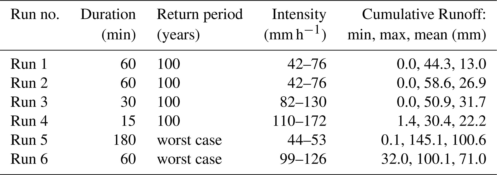
To develop and evaluate overland flow models in the absence of real measurement, artificial sprinkling studies present an opportunity to investigate vegetation effects on overland flow. Table 1 provides information about land use, vegetation properties, and soil characteristics for each site based on Ries et al. (2020) experiment data. The experimental area was a 10 by 10 m square, with slopes ranging from 9 % to 32 %. These experiments aimed to simulate a 100-year or locally observed maximum rainfall intensity event with different durations. Rainfall experiments started with Run 1 on the first day. Subsequently, Run2–Run5 were conducted on the following day and Run 6 was carried out on the third day (Table 2).

Table 1 Properties of experimental sites and the values of constant Manning's roughness coefficient. Paired sites are indicated by boxes and bold font, parameters indicated by * are published in the original dataset (Ries et al., 2020).

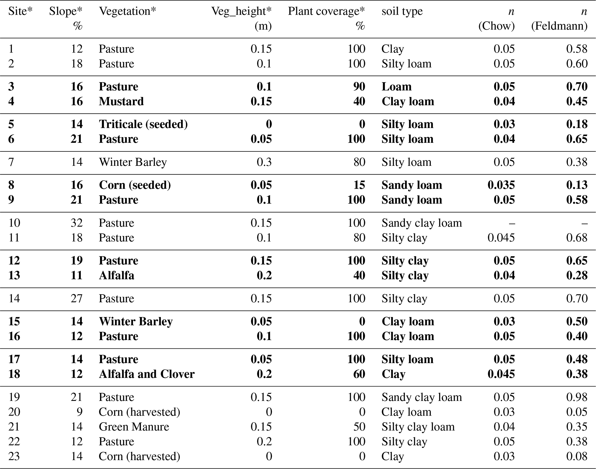
The experiments conducted at Site 10 did not produce any runoff and were not used in this study. Discharge at the outlet, rainfall intensity, and initial soil moisture were measured at a temporal resolution of 1 min. Out of the 23 sites surveyed, 12 locations are paired sites, highlighted in bold in Table 1. This arrangement facilitates a direct comparison between the effects of two different land uses on runoff and infiltration. The deliberate choice of these paired sites is underscored by their proximity, with distances maintained within the threshold of less than 100 m. For more comprehensive details of these experiments, refer to Ries et al. (2020).

Table 2 Characteristics of rainfall for experimental sites (Ries et al., 2020).

2.2 Model

To explore the impact of different roughness functions on overland flow simulations, it is crucial to integrate the relationship between roughness and water depth into the model. For this purpose, OpenLISEM (Open LImburg Soil Erosion Model), which was developed based on the original LISEM (Jetten, 2002), was chosen for its modular structure, physics-based approach and accessibility of the source code, published under a free licence (GNU Public Licence v3, https://github.com/vjetten/openlisem/, last access: 25 August 2026). It is an event-based and spatial hydrological model suitable for different sizes of catchments. It focuses on simulating runoff, sediment dynamics, and infiltration during heavy rainstorms, allowing for detailed assessments of land use changes and conservation measures (Baartman et al., 2012). Artificial elevation models are generated with a cell size of 0.5 × 0.5 m, providing information about the gradient of each specific location in the database (Table 1). Since the mean slope of the experimental plots is constant, spatial variability can be ignored in the model; the generated DEM however does not include microtopography. So, all surface parameters that may influence overland flow are represented within Manning's coefficient. This simplification does not affect our evaluation of different roughness approaches, as the conditions are consistent across all roughness methods. Therefore, the effect of micro-topography was assumed to be inherently reflected in the roughness values. The last row of the DEM colorized black in Fig. 1a represents the trench designed to collect runoff, positioned 40 cm below the surface as in constructed experiments. Figure 1b illustrates the field setup from Ries et al. (2020), which measured flow at three points within the trench. In our model, discharge data is recorded at the outlet, located at the corner end of the trench. Since the trench length to the outlet in the experiments is one-third of that in our model, we compensated by tripling the water velocity in the trench through a reduction in Manning's coefficient for the trench surface.

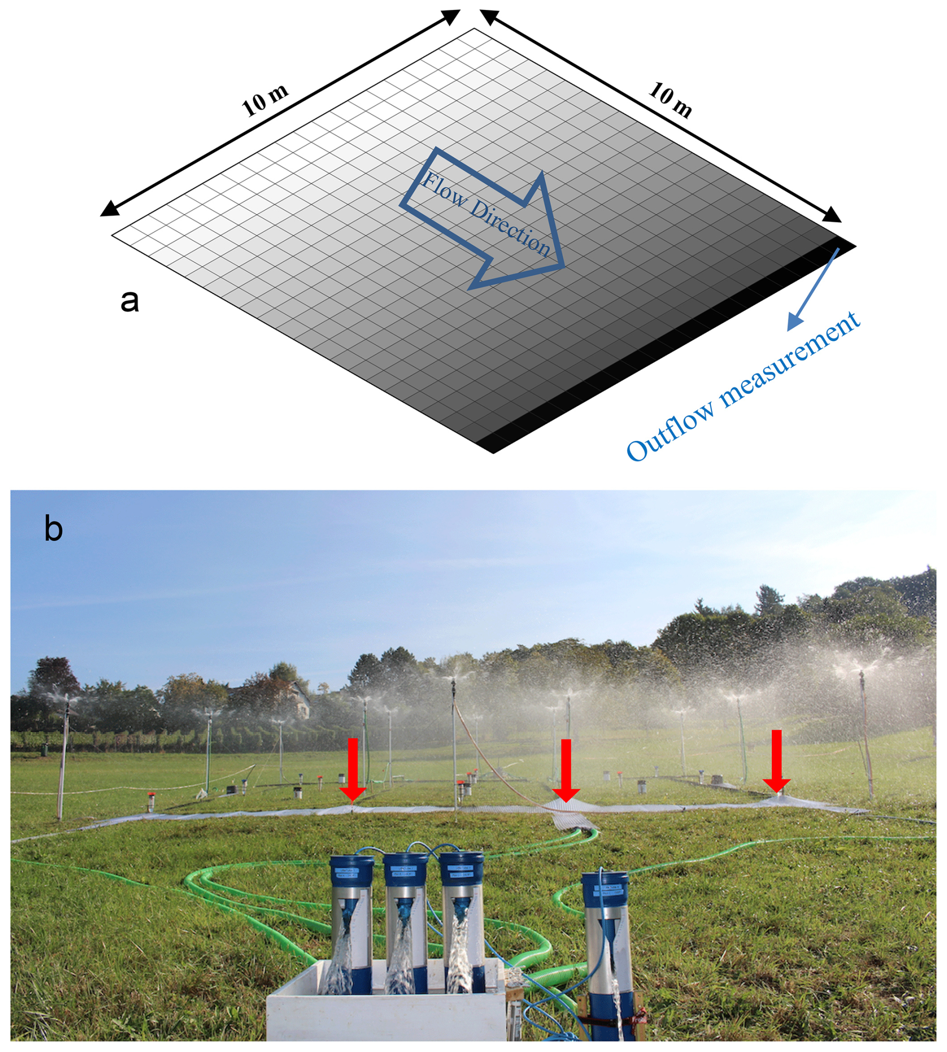
Figure 1 (a) 0.5 × 0.5 m digital elevation model applied for simulations, incorporating the specific slope of each site. (b) Setup of field experiments by Ries et al. (2020). The red arrows indicate the locations of flow collection.

Time resolution for simulation is 1 s and the total simulation time is chosen based on observation runoff data. For the distributed routing of overland flow, a four-point finite-difference solution of the kinematic wave is used together with Manning's equation (Jetten, 2002). Infiltration was estimated using the Green-Ampt method (Rawls et al., 1983), which incorporates field-measured variables such as porosity and initial soil moisture content. Two additional parameters, saturated hydraulic conductivity (K_sat) and average suction at the wetting front (Psi), have not been provided with the dataset. Prior studies, including those by Jetten (2002), Hessel et al. (2003) and Starkloff and Stolte (2014), have highlighted the primary sensitivity of OpenLISEM to K_sat and Psi parameters. Therefore, reasonable ranges for K_sat and Psi were adopted from Rawls et al. (1983), and the values were subsequently calibrated to best match observed runoff data (Sect. 2.3). It should be kept in mind that infiltration in model depends on both soil properties and surface water depth, increased vegetation cover or a higher Manning's roughness coefficient reduces flow velocity, leading to greater surface water depth and, consequently, an enhanced infiltration rate.

OpenLISEM version 6.873 has been utilized which employs Manning's approach to calculate the runoff velocity. While the original software employed a constant Manning's coefficient as a raster map for roughness, a new feature called the dynamic Manning's n function has been introduced into the software to implement different Manning's coefficient estimation methods in simulations. This feature enables users to select from various methods of roughness estimation, including not only a constant value but also methods dependent on the depth of runoff. Detailed information about these extensions can be found in the “Code and data availability” section.

2.3 Flow resistance parameterization

Flow resistance parameterization is a foundational component in simulating overland flow, affecting the accuracy of hydrological models. Roughness estimation approaches represent the resistance of the surface in the model that affects the momentum and energy dissipation of overland flow. OpenLISEM uses the Manning's equation to calculate flow resistance with a constant Manning's n, to be provided by the user. We have extended the code of OpenLISEM (see https://doi.org/10.5281/zenodo.22042844, Kraft, 2026) with five depth-dependent roughness functions (Sect. 2.2.3–2.2.7) and compare the results with two depth-independent Manning's n estimations (Sect. 2.2.1 and 2.2.2).

2.3.1 Constant Manning's coefficient

The initial approach assumes a constant value for Manning's roughness coefficient (n) based on Chow (1959), representing the range of flow resistance for floodplains covered by vegetations. The values of Manning's roughness coefficient using Chow's guideline for each site of the artificial rainfall experiments are given in Table 1. In this method, values are typically selected based on established literature or site-specific calibration. This is suitable for homogeneous surfaces, and it does not consider the dynamic effect of water depth on the roughness coefficient in presence of vegetation.

2.3.2 Robust Manning's coefficient

In the study conducted by Feldmann et al. (2023), the n values were directly iterated within the framework they established. They also used the experimental data and study sites from Ries et al. (2020). The authors reported that the most robust results, characterized by high Nash-Sutcliffe Efficiency (NSE) values, were achieved with constant Manning values, as presented in Table 1. They estimate surface roughness coefficients by analyzing the shape of the hydrograph, fitting the Hortonian equation to the difference between rainfall input and observed discharge for the falling limb of the hydrograph. To achieve this goal, they assumed that the infiltration rate in the descending limb of the hydrograph is constant. For more details, see Feldmann et al. (2023).

2.3.3 Linear method

Drawing on previous literature on artificial grass, including Oberle et al. (2021) concluded that a flow-depth-dependent roughness spectrum can be derived for overland flow, despite inherent variability in the data. Similarly, Hinsberger et al. (2022) found Strickler coefficient, k_Str, values varied with different water depths in the presence of vegetation. Based on their results, there are three zones to specify roughness within the data range, categorized according to the submergence ratio: for emergent and fully submergent zones they emphasis the roughness is constant.

A linear function of relative submergence can be described for the roughness coefficient between emergent and fully submergence zones ($\mathrm{1}<\frac{h}{h_{\mathrm{veg}}}<\mathrm{5}-\mathrm{7}$) (Hinsberger et al., 2022).

These relationships are summarized in Eq. (1):

$$\begin{array}{}\text{(1)}& \mathrm{1}/n_{\mathrm{Manning}}=\left\{\begin{array}{ll}\frac{k_{\mathrm{Str}}}{\mathrm{5}}& \text{for}\mathrm{0}<h<h_{\mathrm{veg}}\\ \frac{k_{\mathrm{Str}}}{\mathrm{5}}+k_{\mathrm{Str}}\frac{h-h_{\mathrm{veg}}}{\mathrm{5}}& \text{for}{h}_{\mathrm{veg}}<h<\mathrm{5}{h}_{\mathrm{veg}}\\ k_{\mathrm{Str}}& \text{for}h>\mathrm{5}{h}_{\mathrm{veg}}\end{array}\right.\end{array}$$

The parameter $k_{\mathrm{Str}}=n_{\mathrm{Manning}}^{-\mathrm{1}}$ is Strickler's coefficient which is the inverse of the roughness coefficient above the vegetation using Chow (1959). Then Manning's coefficient is calculated from Eq. (1), depending on the submergence ratio.

2.3.4 Luhar and Nepf's method

Another method to investigate vegetation effect on roughness was proposed by Luhar and Nepf (2013) for open channel. They suggested the following relationships between the Manning roughness caused by vegetation and blockage factor, B_x, for both submerged and emergent vegetation.

$$\begin{array}{}\text{(2)}& n_{\text{Manning-veg}}=\left\{\begin{array}{l}\frac{K{h}^{\frac{\mathrm{1}}{\mathrm{6}}}}{g^{\frac{\mathrm{1}}{\mathrm{2}}}}{\left(\frac{C_f}{\mathrm{2}}\right)}^{\frac{\mathrm{1}}{\mathrm{2}}}{\left(\mathrm{1}-B_x\right)}^{-\frac{\mathrm{3}}{\mathrm{2}}}\\ \text{for}h\le h_{\mathrm{veg}}\wedge B_x<\mathrm{0.8}\\ \frac{K{h}^{\frac{\mathrm{1}}{\mathrm{6}}}}{g^{\frac{\mathrm{1}}{\mathrm{2}}}}{\left(\frac{C_{\mathrm{d}}ah}{\mathrm{2}}\right)}^{\frac{\mathrm{1}}{\mathrm{2}}}\\ \text{for}h\le h_{\mathrm{veg}}\wedge B_x\ge \mathrm{0.8}\\ \frac{K{h}^{\frac{\mathrm{1}}{\mathrm{6}}}}{g^{\frac{\mathrm{1}}{\mathrm{2}}}}\frac{\mathrm{1}}{{\left(\frac{\mathrm{2}}{C_f}\right)}^{\frac{\mathrm{1}}{\mathrm{2}}}{\left(\mathrm{1}-\frac{h_{\mathrm{veg}}}{h}\right)}^{\frac{\mathrm{3}}{\mathrm{2}}}+{\left(\frac{\mathrm{2}}{C_{\mathrm{d}}a{h}_{\mathrm{veg}}}\right)}^{\frac{\mathrm{1}}{\mathrm{2}}}\left(\frac{h_{\mathrm{veg}}}{h}\right)}\\ \text{for}h>h_{\mathrm{veg}}\end{array}\right.\end{array}$$

where n_Manning-veg is the vegetation component of Manning's n, a is the frontal area per unit volume parameter, and C_d is drag coefficient. We assumed that the stem of vegetation is cylindrical in shape, and therefore a C_d value of 1 was used. $C_f(=\mathrm{0.015}-\mathrm{0.19})$ is a coefficient to parameterize the shear stress at the interface between vegetated and unvegetated regions and the constant K=1 m${}^{\mathrm{1}/\mathrm{3}}$ s⁻¹ is required to make the equation dimensionally correct. The other parameters will still be the same. Although the equation was originally proposed for channel flow, this study examines its applicability to overland flow.

2.3.5 Exponential method

Following Feldmann et al. (2023), Manning's roughness coefficient is parameterized as a reciprocal exponential function of water depth, enabling systematic exploration of different roughness–depth relationships. A reciprocal formulation was selected to ensure a more balanced sampling of roughness functions across the parameter space, thereby preventing the under representation of low roughness values. The exponential equation describes the relationship between n and h in terms of the variables c and d (Eq. 3).

$$\begin{array}{}\text{(3)}& n={\displaystyle \frac{\mathrm{1}}{c+e^{dh}}}\end{array}$$

The optimum values of the c and d parameters for each location were derived from the study by Feldmann et al. (2023), whose proposed approach is explained in Sect. 2.2.2.

2.3.6 Kadlec's method

Based on experimental studies on overland flow, Kadlec's power law was simplified by Jain et al. (2004) (Eq. 4).

$$\begin{array}{}\text{(4)}& n=n_{\mathrm{0}}{\left({\displaystyle \frac{h}{h_{\mathrm{0}}}}\right)}^{-\mathit{ϵ}}\end{array}$$

where h₀ establishes the minimum flow depth, beyond which the roughness coefficient n₀ is assumed to remain constant. ϵ represents the influence of vegetation drag. Our study utilized the optimal values for the parameters n₀ and ϵ as outlined in Feldmann et al. (2023). As they did not provide information on the h₀ value, we assigned h₀ to be five times the plant height, as indicated by the lab experiments by Hinsberger et al. (2022).

2.3.7 Fu's equation

Fu et al. (2019) developed an equation to calculate Manning's n based on plant basal cover and flow depth (Eq. 5).

$$\begin{array}{}\text{(5)}& n=\left(a+b{\left(\mathrm{1}-e^{-\mathrm{0.061}{C}_v}\right)}^{\mathrm{1.668}}\right)h^{\mathrm{0.604}-\mathrm{0.710}{e}^{-\mathrm{0.219}{C}_v}}\end{array}$$

Where C_v is the vegetation coverage (plant basal cover) inside of a flume. The coverage varied between 1.25 % to 30 % in the lab experiments by Fu et al. (2019). For the transition of the equation to surface runoff, we are using the value “plant coverage” from the Ries et al. (2020) dataset, but with the uncertainty, that the basal coverage is usually lower than the total coverage. The parameters a and b vary with vegetation type. In this study, the values of a and b parameters obtained by Feldmann et al. (2023) are used. These equations were incorporated into the source code of OpenLISEM to assess the impact of various roughness methodologies on overland flow modelling.

2.4 Parameter calibration and validation

To compare the different roughness equations, we calibrate the unknown sensitive parameters of the model using one of the six rainfall experiments (Run) per site, (cf. Table 2), and validate the parameters using the remaining rainfall experiments. For most locations, run 2 (100-year return period event, prewetted soil) was selected as the calibration event. Runs 1, 3, 4, 5, and 6 were selected as validation experiments. The reason for choosing Run 2 for calibration was that the soil moisture conditions during this test were neither excessively dry. Since Run 2 in site 14 does not have any runoff, Run 6 is selected for calibration. Site 1 has a different order of experiments, so we are using Run 4 as the calibration run. The most sensitive parameters saturated conductivity (K_sat) and average soil suction at the wetting front (Psi) are calibrated for 23 sites and 7 different roughness approaches (154 models). The parameters for the roughness functions are selected as described above and Manning's n is selected from the well-known Chow-Table (Chow, 1959). For sites with dense vegetation (e.g., close to 100 % cover), higher values within the range reported by Chow (1959) were assigned, whereas for sites with sparse or no vegetation, lower values were used. To assess the effect of these preselected values, we added Manning's n as an additional parameter, adding one model per location with 3 calibrated parameters (total 176 models).

The calibration was performed with 5000 simulations per model (880 000 models) with a distribution of the 2 or 3 parameters using the latin hypercube sampling (LHS) method using the implementation in SPOTPY (Statistical Parameter Optimization Tool) (Houska et al., 2015). The saturated hydraulic conductivity (Ksat) varies between 5 and 100 mm h⁻¹, and the wetting front suction head (Psi) ranged from 0 to 50 cm water column, both within the ranges suggested by Gowdish and Muñoz-Carpena (2009) for different soil types. The broad range is selected to account for the variability of natural soils, especially in the presence of macropores.

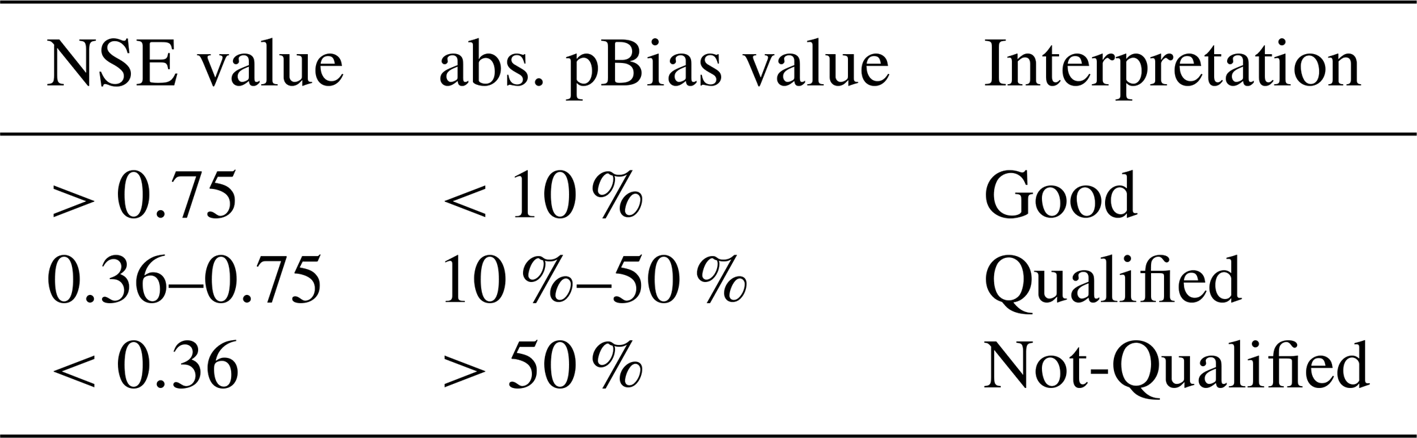
The best calibrated parameters are selected by ranking the model runs by their Nash-Sutcliffe efficiency (NSE). After calibrating the K_sat and Psi, models were developed for the rest of the experiments. The validation performance is reported as NSE and relative bias in percent (pBias) (Table 3). High positive NSE values (close to 1) indicate that the model's predictions are in excellent agreement with the observed data. pBias with values closer to zero indicating better model performance. An ANOVA test was performed to check, if calibrated values of K_sat and Psi are significantly influenced by the chosen roughness method as an unwanted side effect. Model validation results from all sites and experimental runs were compared among the roughness estimation methods to evaluate their overall performance. The effect of vegetation on infiltration was assessed by comparing the calibrated K_sat values between paired sites. In addition, the influence of initial soil moisture on runoff modeling was examined by comparing NSE values across all runs at each site.

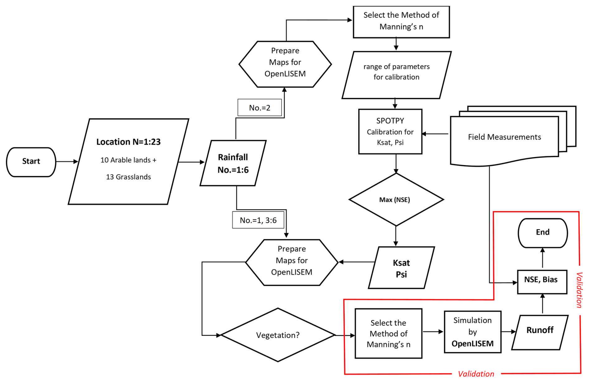
Figure 2 displays a framework illustrating the calibration and simulation process of models. The simulations were iteratively repeated, considering all methods of roughness estimation. A total of 104 runs were simulated, each representing different sites or rainfall events, and repeated for various roughness methods, resulting in 832 simulations. However, models associated with Run 2 and 3 at Site 14, as well as Run 1 at Sites 12 and 16, were excluded from NSE assessment due to the absence of runoff in these experimental runs. Since the observed data were zero, the NSE could not be calculated. Nevertheless, based on a comparison between the simulated hydrographs and the corresponding NSE values, the differences between the simulations and observations indicate that the model performance is acceptable.

Table 3 Criteria of NSE value (Motovilov et al., 1999) and pBias.

Figure 2 Framework for calibration and validation of the models.

2.5 Initial soil moisture

Initial soil moisture plays a critical role in hydrological modeling, as it directly influences the partitioning between infiltration and surface runoff (Lin et al., 2024; Shahrban et al., 2018). Soil moisture measured at two points at each site was used in the runoff modeling. In addition, the sequence of six rainfall-runoff experiments (Runs 1–6, as shown in Table 2) was considered, which involved varied antecedent moisture conditions, ranging from dry to saturated. This experimental design provides a general representation of initial soil moisture states. Therefore, in addition to point-based measurements, considering the antecedent moisture conditions of each run enhances the interpretation of simulation results and improves understanding of the hydrological model's response.

2.6 Comparison of paired sites

The dataset by Ries et al. (2020) uses partly a paired site approach (Table 1). The paired sites are in close spatial proximity, have similar soils but different vegetation covers. We are using these site pairs to compare the results with and without vegetation to account for vegetation effects on model performance. Due to the great efforts needed to conduct rainfall simulation experiments, the dataset of Ries et al. (2020) is one of the most comprehensive collections with repeated methodology, but in effect, only six paired sites exist.

3 Results

3.1 Calibration of K_sat and Psi for different roughness methods

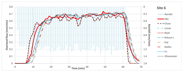
During the calibration process using various roughness estimation methods, the simulated hydrographs generally aligned well with observed hydrographs across most sites. For instance, Fig. 3 compares the calibrated hydrographs at site 6, where simulated results successfully capture the temporal pattern of measured discharge for other sites; the results are presented in supplementary data. The NSE values for all sites are summarized in Fig. 4. Additionally, the pBias values, computed using the calibrated K_sat and Psi parameters, are presented in Fig. 5. A high absolute pBias typically indicates a less accurate calibration.

At sites with high model performance, the different methods yield similar results. However, while using Fu's method, the calibration failed (NSE<0) at the sites without vegetation (5, 15, 20, 23) and at the site with scarce vegetation (site 8 with 15 % plant coverage), cf. Table 1. The other methods performed well at these sites. Unfavorable calibration performance was also observed at Sites 11 and 16, where all roughness estimation methods produced relatively low NSE and pBias values. It indicates a significant discrepancy between the observed and simulated hydrographs.

In contrast, the remaining sites showed satisfactory calibration results using all methods except Fu's. Excluding Sites 11 and 16, the NSE values across other locations, except Fu's method, generally ranged between 0.65 and 0.87, reflecting an acceptable level of model performance.

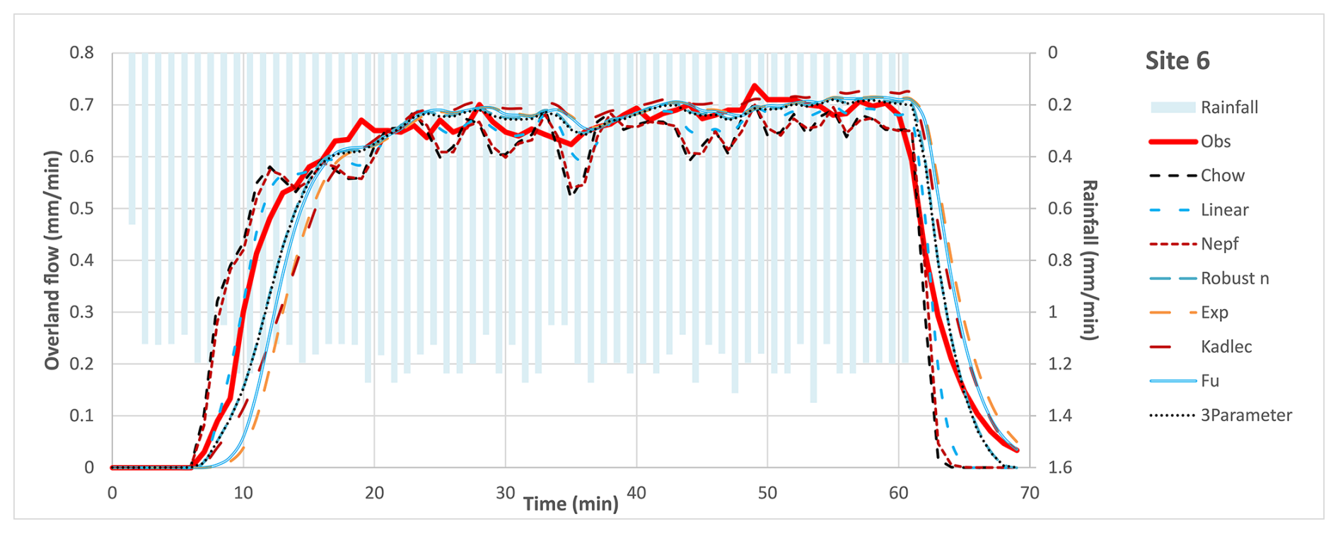
Figure 3 Comparison of the hydrograph computed using OpenLISEM with various roughness coefficient methodologies against the observed discharge.

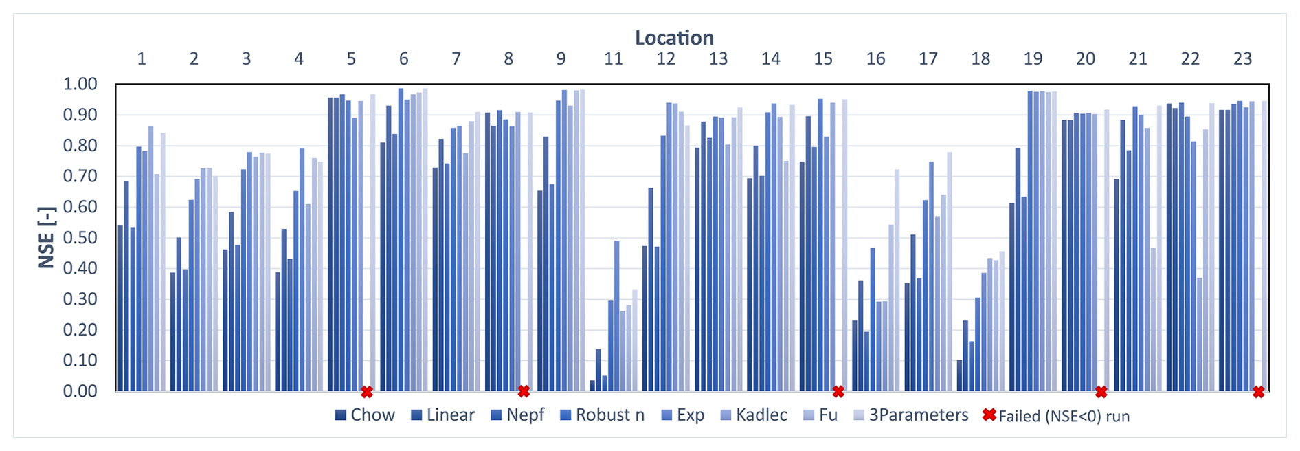
Figure 4 Maximum model performance (Nash-Sutcliffe-Efficiency) for the calibration runs of the different roughness models, separated for each site. The red bars show model failure.

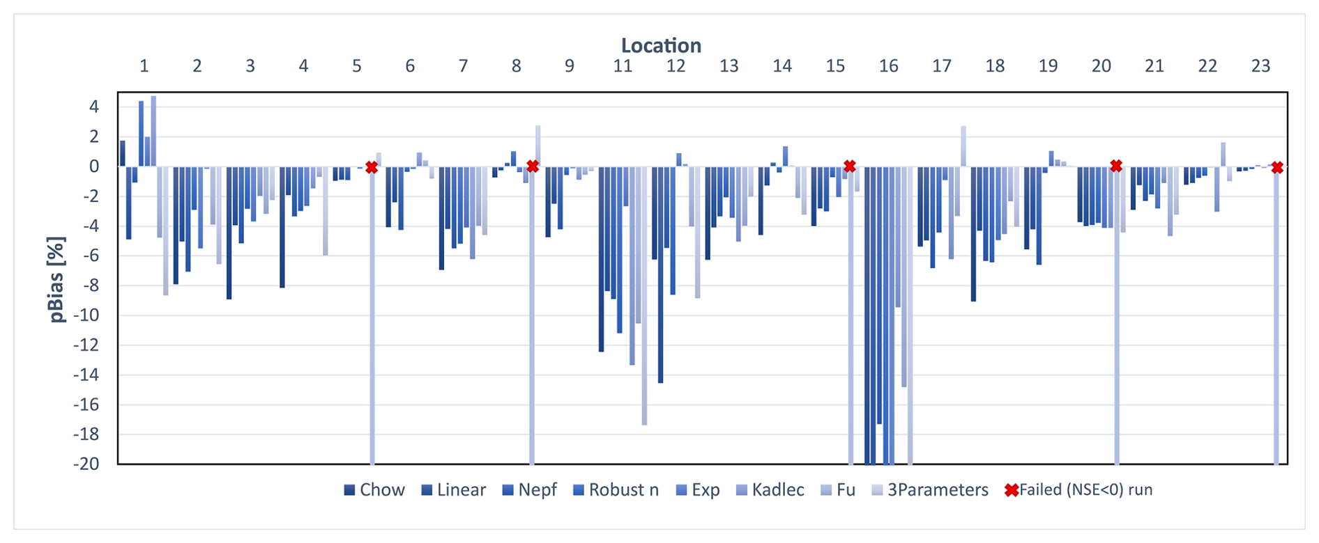
Figure 5 pBias values for parameters calibration of the different roughness models, separated for each site. Rainfall simulation Run 2 has been used for calibration, except for sites 1 and 14 (see Sect. 3).

Runoff is generally underestimated by the model, only 13 % of the runs show a slight overestimation (<5 % bias). 59 % of the model runs underestimate the measured runoff by less than 5 %, while 21 % of the runs are underestimated by 5 %–15 % of the runoff. Massive underestimation of runoff (>15 %) happens outside at 5 runs using Fu's equation for surface roughness, while the runoff at site 16 is underestimated by most model runs, which is connected to the low total runoff at this site.

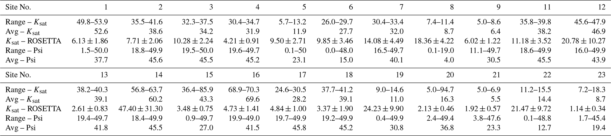
presents a summary of the calibrated values of K_sat and Psi, calculated using different methods across all sites. In the case of Fu's method, the K_sat values for sites 5, 8, 15, 20, and 23 differ significantly from those obtained using other methods. These discrepancies suggest that Fu's method does not perform well in calibrating K_sat at these specific sites. The highly negative NSE values of the Fu method at these sites further support this observation. Additional results are presented in detail in the supplementary data.

A comparison of K_sat values shows that the differences between roughness methods are generally not significant, p-value = 0.94, across sites. However, the values of Psi for different roughness methods show differences, p-value = 0.038.

Table 4 Statistical summary of calibrated parameters, Ksat (mm h⁻¹) and Psi (cm), by site for different roughness methods. For reference, Ksat values estimated with the ROSETTA3 tool (Zhang and Schaap, 2017) from soil texture and bulk density are given.

3.2 Validation of different roughness methods

The outcomes of validation reveal that the maximum NSE range is 0.96–0.98 for different methods. By considering validation results for all sites and all runs for each roughness estimation method, we found that depending on the type of method, the number of models with negative NSE varies between 29 and 46, of which most of them are Run 1 and Run 5. Given that greater NSE values indicate more efficiency of the model in simulating runoff, we focused our investigation on the distribution of positive NSE values by excluding these underperforming models. Figure 6 illustrates the distribution of NSE for values greater than zero. The results indicate that the Linear and Nepf methods perform better in estimating runoff compared to the other methods; however, the differences are not statistically significant. ANOVA analysis on NSE values reveals significant differences between all group means, including Fu and Exp (p-value = 1.3e−11). In contrast, when excluding Fu and Exp from the analysis, no significant differences are observed among the remaining roughness methods (p-value = 0.4).

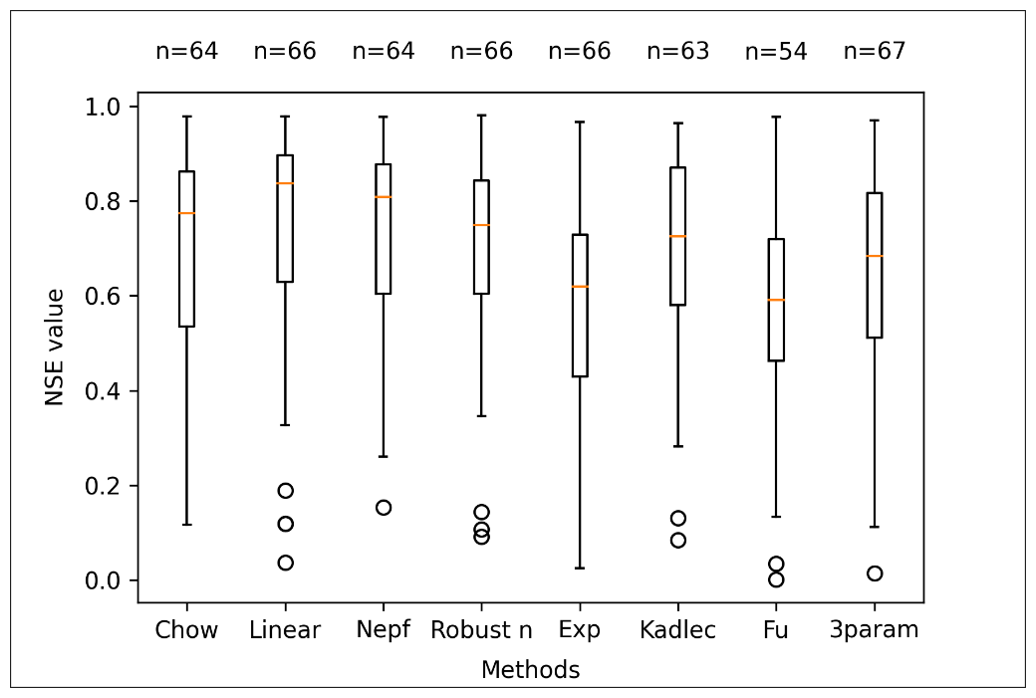
Figure 6 Distribution of the absolute values of NSE for each method of roughness for the validation runs.

The pBias results for the simulated hydrograph compared to the measured hydrograph exhibit a broad range from −100 % to 100 % in Fig. 7. It is evident that all the methods exhibit almost a consistent trend, with the majority showcasing model bias consistently below zero. This suggests an underestimation across various roughness estimation methods. However, ANOVA analysis of the pBias values for all methods excluding Fu indicates no statistically significant difference between group means (p-value = 0.99).

Figure 7 Distribution of the pBias for each method of roughness for the validation runs.

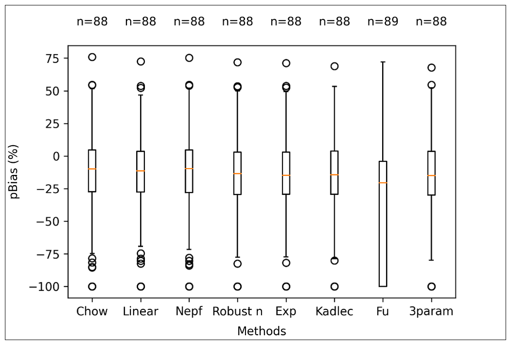
The analysis reveals that the Nepf, Linear, and Chow methods exhibit the most favorable performance, with 39, 38, and 34 models falling into the “Good” category based on NSE values. Conversely, for Robust n, Kadlec, 3-parameter, exponential, and Fu methods, 33, 29, 25, 15, and 9 models respectively meet the “Good” NSE criteria. Interestingly, pBias values across different methods are relatively comparable. Nepf, Chow, Linear, and 3-parameter demonstrate particularly robust performance, each with 27, 27, 26, and 26 models falling within the −10 % to 10 % bias range. This consistency in bias values suggests a commendable performance by these models based on pBias criteria.

3.3 Effect of initial condition and pre-event soil moisture

The validation outcomes of the roughness methods revealed Run 1 (dry conditions) and Run 5 (saturated conditions) generally shows poor model performance, with most of the methods. From the 36 model runs with negative NSE using the Nepf method, 30 are from Runs 1 and 5, as an example. Run 1 tends to overestimate runoff (positive pBias), while Run 5 underestimates it (negative pBias). The extremely low observed runoff in Run 1 makes NSE highly sensitive and often unreliable. On the other hand, these weak performance for Runs1 and Runs 5 in comparison others may because of the difference on the initial condition of models with Run 2 which was selected for calibration.

3.4 Result of different vegetation coverage

The spatial proximity between the paired experimental sites offers a unique advantage in the research, providing an environment where variations in soil characteristics can be minimized, enhancing the validity of the comparative analysis.

In Fig. 8, a comparative analysis between vegetation cover and K_sat, as determined by the Chow method, is presented. Comparing the pair sites reveal an increase in K_sat corresponding to more vegetation coverage. Notably, the contrast in K_sat is particularly pronounced between sites 15 and 16. Site 15, characterized as devoid of vegetation cover, displays a stark difference from site 16, boasting 100 % vegetation coverage. The calibration results underscore this disparity, indicating a substantial K_sat difference of approximately 30 mm h⁻¹ Conversely, for sites 8 and 9, this difference in K_sat is minimal. It's noteworthy that, although K_sat values may show only slight differences, another critical parameter influencing infiltration, Psi, exhibits a substantial contrast between sites 8 and 9. As presented in Table 4, the average of Psi value in site 9 is 30.5 cm; however, this value for site 8 is 4 cm. Specifically, Psi is higher for site 9 than site 8, resulting in an enhancement in infiltration. This highlights the relationship between various parameters and their combined impact on the overall dynamics of infiltration.

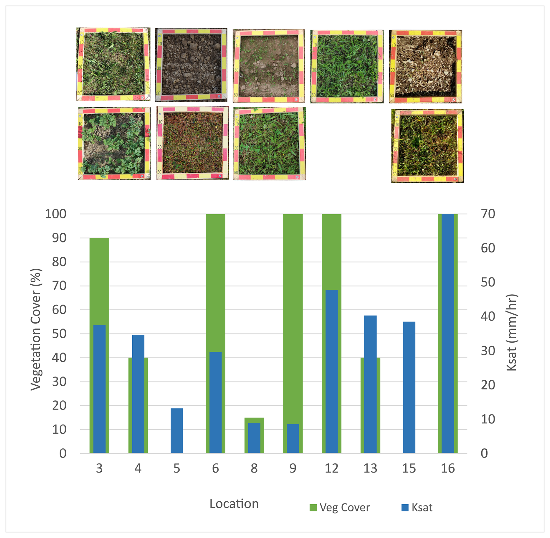
Figure 8 Saturated hydraulic conductivity values for various land uses in paired sites. ** The vegetation cover images are from Ries et al. (2020). There is no picture for Site 13.

As an example, the results for pair sites 12 and 13 are shown in Fig. 9. Site 12 with 100 % vegetation cover and site 13 with 40 % show different hydrographs both in observation and simulation. The results for Runs 2, 3, 4, and 6 are presented in this figure. For these runs, except Run 6 in Location 13, the model performs well, and the differences between observed and simulated values are not significant, the result for the other paired locations are shown in the supplementary material (Masoodi and Kraft, 2025). In these figures solid lines show the observed hydrographs and the shaded areas show the spread of results from different roughness methods. The green shaded area shows the results for the location with more vegetation cover. The spread of simulations is much larger for location 13, with less vegetation. It means in the presence of vegetation; the infiltration rate is higher than in places with less vegetation cover.

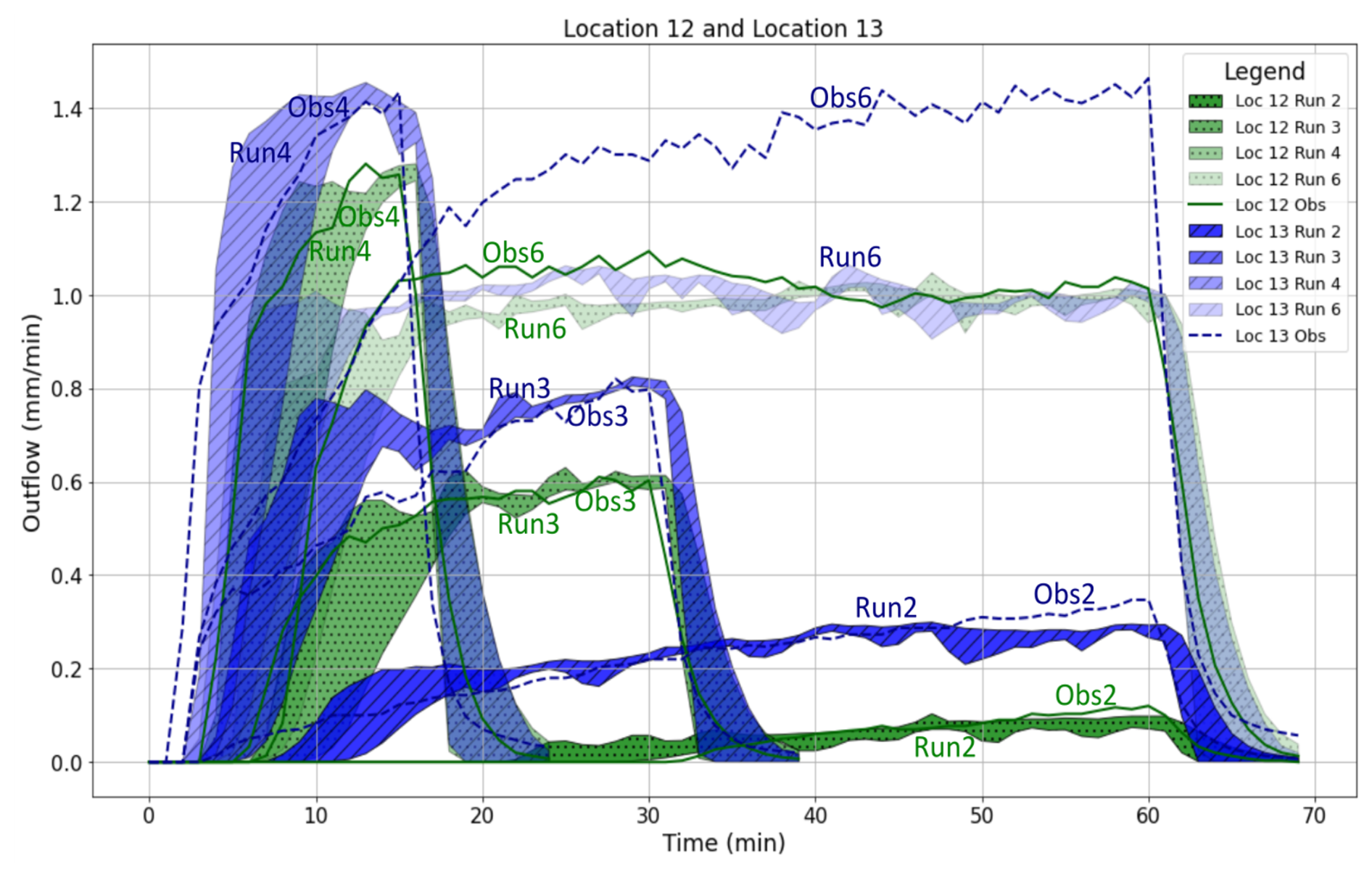
Figure 9 Comparison of observed, solid lines, and simulated hydrographs, shaded areas, at sites 12 and 13 using different roughness methods for Run2, 3, 4, and 6.

An example illustrating the model results with weak performance in Runs 1 and 5 is presented in Fig. 10, which shows the outcomes for Sites 12 and 13. As discussed previously, most models perform poorly for these two runs. A comparison between Figs. 9 and 10 indicates that the weak performance in Runs 1 and 5 is not related to either the infiltration modeling or the roughness approach. This conclusion is supported by the fact that the infiltration modeling in the other runs (2, 3, 4, and 6) shows acceptable agreement between observed and simulated values. The different roughness methods cannot account for the large discrepancies observed.

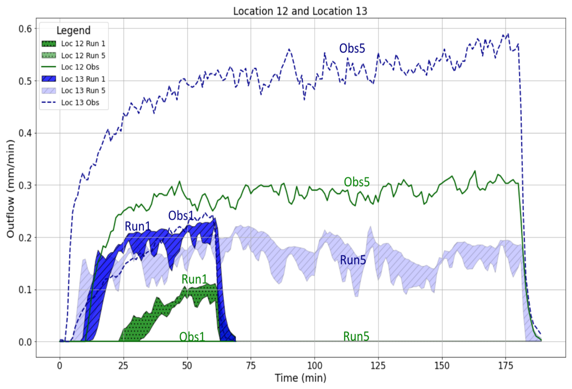
Figure 10 Comparison of observed, solid lines, and simulated hydrographs, shaded areas, at sites 12 and 13 using different roughness methods for Run 1 and Run 5.

4 Discussion

4.1 Applying a catchment model on a plot experiment

A catchment model can only be applied to a small-scale field experiment with some workarounds and assumptions, leading to additional sources of uncertainty. First, differences between the experimental setup and the model representation introduce structural uncertainty. In the field experiments (Ries et al., 2020), runoff was collected using a trench and drainage tube system, whereas in the model, discharge is recorded at a defined outlet cell. Although adjustments were made to approximate the experimental conditions, the simplified representation of the measurement may influence the comparison between simulated and observed results. Second, the model does not explicitly represent small-scale heterogeneities such as the spatial distribution of vegetation, microtopography, or preferential flow paths. These factors can significantly affect overland flow and infiltration processes in real field conditions but are represented in the model only by a simple surface retention factor. Third, the temporal resolution of the experimental data (1 min). While the relatively uniform rainfall intensity and duration of the events suggest that the available resolution is sufficient, higher resolution would give us more detailed information about the hydrological process. Forth, the infiltration modelling approach (Green–Ampt) assumes simplified soil conditions, which may not fully represent complex field situations, particularly under very dry or near-saturated initial soil moisture conditions. This limitation is reflected in the reduced model performance for extreme antecedent conditions (e.g., Runs 1 and 5). However, using any explicit infiltration model for runoff modelling is already a great improvement in comparison to the still common “effective rainfall” approach based on the curve-number approach, where the estimated infiltration is simply subtracted from the rainfall, as it allows infiltration of water that has already travelled at the surface.

Differences between modelling approaches can further contribute to variations in results. For example, the model setup used in this study and the framework proposed by Feldmann et al. (2023) rely on different assumptions regarding roughness parameterization, calibration strategies, and representation of hydrological processes. These methodological differences, combined with the inherent uncertainties in both models and measurements, may partly explain the observed discrepancies between the results.

4.2 Validation of different roughness methods

Our study on the validation of various roughness estimation methods revealed that models using Fu's function yielded comparatively weaker simulation results compared to experimental data. This finding is consistent with Feldmann et al. (2023), who reported that Fu's equation typically produces lower NSE values, attributed primarily to the formula's limited adaptability. This limitation may stem from the fact that the function was developed based on laboratory experiments and is most applicable under similar controlled conditions where plant basal cover varied between 1.25 % and 30 %. The method fails at the unvegetated site (5, 8, 15, 20 and 23) and at the sparsely vegetated site 8. Fu's function should be used only for patchy vegetated flumes, as intentended by the authors and not for sheet flow regimes. In contrast, models based on Nepf, Linear, Chow, and Robust n methods, ranked in that order, demonstrated a closer match between the simulated and observed hydrographs. Although the differences in NSE values among these latter methods are not substantial, their use in roughness estimation leads to simulated hydrographs that more closely represent those derived from physical observations. One notable strength of the Nepf and Linear methods is their incorporation of water-depth-dependent relationships in estimating roughness coefficients. This is in agreement with Hinsberger et al. (2022), who emphasized the critical role of water depth in influencing hydraulic roughness and highlighted the importance of integrating this factor into catchment-scale modeling. It should be noted that in our simulations, water depth remained below 20 mm (except for the failed runs with Fu's method), placing the system in an emergent flow regime (see supplemental material). Under this condition, the performance of the applied methods is considered valid; however, further investigation is required to assess their accuracy under submerged flow conditions. Additionally, the improved performance of the Nepf method may also be attributed to its inclusion of the blockage factor, which effectively represents vegetation cover and enhances the simulation of overland flow. Although originally (Luhar and Nepf, 2013) developed for channel flow, the Nepf method demonstrates strong alignment with physically measured hydrographs in overland flow scenarios as well (Luhar and Nepf, 2013). Therefore, further research is warranted to assess and refine its applicability in such contexts.

Our results using the 3-parameter method indicate that increasing the number of parameters during calibration can lead to greater model complexity, which may hinder the ability to efficiently identify optimal solutions. This increase in complexity can also negatively impact overall model performance. Similar findings have been reported in previous studies involving conceptual rainfall-runoff models. For instance, Zhu et al. (2024) concluded that increasing model complexity by adding more parameters often leads to challenges in calibration, including difficulty in parameter estimation and reduced calibration efficiency. Likewise, García-Romero et al. (2019) calibrated three hydrological models with varying levels of complexity, comprising 4, 10, and 16 parameters, across nine catchments. Their results demonstrated that simpler models required fewer iterations to reach convergence, whereas more complex models demanded significantly more computational effort.

The results of methods in which roughness values are derived using the approach of Feldmann et al.'s (2023) concept, including Kadlec, Robust n, Fu, and exponential, tend to exhibit greater deviation from experimental data. Figure 11 illustrates a comparison of the simulated hydrographs using different roughness estimation methods for all experiments conducted at site 9. Site 9 is specifically chosen because its hydrographs were featured in Feldmann et al.'s (2023) study, and the calibration for the four methods employed therein is superior to that of the Linear and Nepf methods, as depicted in Fig. 4. Figure 11 demonstrates that Kadlec, Robust n, Exponential, and Fu methods approximate the falling limb of the hydrograph more closely to the observed hydrograph compared to the Linear, Nepf, and Chow methods. It's essential to note that the base of optimization in Feldmann et al. (2023) study is on the falling limb of the hydrograph, where it shows superior performance. However, the NSE results for the entire hydrograph are better for Nepf, Linear, and Chow.

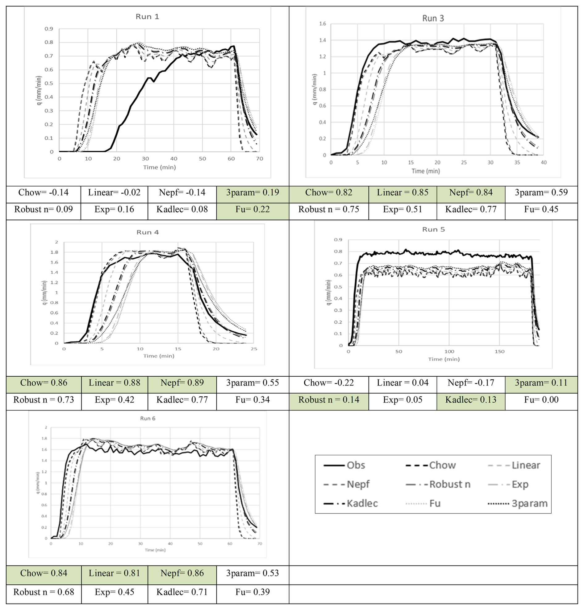
Figure 11 Comparison of validated and observed hydrographs at site 9. NSE values are calculated for the entire hydrograph, with green cells indicating methods that have higher NSE values.

This discrepancy may stem from the approach's omission of vegetation effects on infiltration parameters. Feldmann et al. (2023) proposed a more constrained roughness estimation method by identifying overlapping solution spaces and reducing the overall solution space to enhance reliability. Their methodology focuses on the falling limb of the hydrograph, where infiltration is assumed to remain relatively constant. They fitted an infiltration function to this segment of the hydrograph and derived infiltration rates without explicitly considering vegetation's role in modifying these rates. However, our findings suggest that vegetation significantly influences not only roughness coefficients but also key infiltration parameters, such as K_sat, thereby affecting overall infiltration dynamics. By considering the soil type at each location and comparing the calibrated K_sat and Psi values with the estimates provided by Rawls et al. (1983), it becomes evident that the calibrated values are consistently higher across all sites. The only exceptions are Sites 8 and 9, which have sandy loam soils; in these cases, the calibrated values closely match those estimated by Rawls et al. (1983). Using the ROSETTA3 tool for soil property estimation (Zhang and Schaap, 2017) using the measured soil texture and bulk density, 8 locations have calibrated K_sat values inside of two standar deviations of the ROSETTA results, while 14 locations have calibrated values exceeding two times standard deviation of the ROSETTA values. Since this discrepancy occurs across all roughness function methods, it suggests that the difference is not related to the choice of roughness method. Rather, it highlights a potential limitation of applying simplified, texture-based infiltration parameters to complex field conditions. Factors such as macropores or root development may influence soil hydraulic behavior and lead to higher infiltration rates than those predicted using generalized soil texture classifications (Beven and Germann, 1982).

These results are consistent with the conclusions of Gao et al. (2023), who emphasized that soil hydraulic properties are influenced by both water movement and ecosystem activity. Previous studies highlighted the root zone as a critical component with substantial storage capacity, playing a key role in regulating how precipitation is partitioned into streamflow (Gao et al., 2023; Ponds et al., 2025; Stocker et al., 2023). According to their framework, vegetation actively alters soil characteristics to optimize water availability, which underscores the importance of incorporating ecosystem and soil interactions into hydrological modeling. Similarly Liu et al. (2025) have stated that vegetation indirectly increases the soil's hydrological capacity by directly improving its physical and chemical properties. While K_sat is easily measurable, the effect is also true for the Psi parameter and can hence lead to widely differing chosen parameter ranges for similar soils with different vegetation or management practices. A good example is the site pair 8/9.

4.3 Effect of initial condition and pre-event soil moisture

Our results highlight the significant influence of antecedent soil moisture conditions on runoff modeling accuracy, particularly in Runs 1 and 5. Run 1 began with unusually dry soil, while Run 5 followed a sequence of moderate rainfall events (Runs 2, 3, and 4), although the measured soil moisture does not differ substantially between run 4, 5 and 6. Both exhibited significant deviations between simulated and observed runoff, suggesting that the model struggled to replicate hydrological responses under extreme antecedent moisture states.

These findings are in agreement with Brocca et al. (2008), who demonstrated that pre-event soil moisture is a key determinant of runoff depth and peak discharge. Their conceptual soil water balance model incorporates Green-Ampt infiltration and a non-linear drainage mechanism. In our study, models calibrated under a specific initial moisture condition (e.g., Run 2) yielded more reliable results when validated against runs with comparable antecedent states (e.g., Runs 3, 4, and 6). However, performance declined when these models were applied to scenarios with contrasting initial soil moisture (e.g., Runs 1 and 5), emphasizing the model's sensitivity to calibration context. Feldmann et al. (2023) observed a decrease in median deviation from the roughness mean in Run 5 during prolonged rainfall events and attributed this to the formation of flow paths influencing roughness values. However, we suggest that this reduction may be linked to the effects of antecedent rainfall on runoff response, and not to rainfall intensity or flow path development. This is supported by the behavior in Run 6, where the deviation from the roughness mean increased again despite continued rainfall, indicating that the changes are not solely due to flow path formation.

Zehe and Blöschl (2004) investigated how uncertainty in initial soil moisture affects hydrologic responses at the plot and catchment scales, using a physical model that accounts for transitions between matrix and preferential flow. Their simulation results showed that model predictability is lowest near the soil moisture threshold separating these flow regimes in the soil. In the present study, Runs 1 and 5 represent transitional soil moisture conditions similar to those reported by Zehe and Blöschl (2004). Comparing the results of these runs highlight the difficulty of accurately predicting hydrological responses under uncertain initial soil moisture conditions. These findings are consistent with Zehe and Blöschl (2004).

We found that the response of our model under different soil moisture conditions has uncertainty, particularly when soil approaches saturation. This discrepancy may stem from limitations in infiltration modeling under these conditions. For example, the Green–Ampt approach assumes an initially dry soil profile, which can result in unrealistic infiltration estimates during high-intensity storms on already wet soils. This limitation highlights the need for improved infiltration models that better accommodate a range of antecedent soil moisture conditions.

4.4 Result of different vegetation coverage

These differences result in different shaping perched water table dynamics and overland flow responses (Ghimire et al., 2020; van Meerveld et al., 2021; Zwartendijk et al., 2020, 2023). The study conducted by Wu et al. (2024) on the temporal variability of K_sat throughout the growing season revealed the significant influence of root growth. They explained that root development improves soil pore connectivity, thereby increasing K_sat. Consequently, top-soil infiltration rates typically experience improvement, resulting in reduced overland flow and a decrease or delayed runoff response to rainfall events (van Meerveld et al., 2019). Jarvis et al. (2013) identified land use as one of the top three most significant predictors for K_sat. They concluded that intensive cultivation of arable land significantly diminishes topsoil hydraulic conductivity compared to perennial agriculture, natural vegetation, and forests, by approximately 2–3 times. They attributed this reduction to the disruptive effects of tillage on macropores, including faunal and root bio pores.

Our research indicates that in the presence of vegetation, not only is surface roughness important in hydrological processes, but the increase in K_sat also significantly influences the response of hydrological models to runoff. This highlights the critical importance of incorporating vegetation-induced changes in hydraulic conductivity when modeling runoff responses. A great difference from the related studies by Feldmann et al. (2023) and Hinsberger et al. (2022) is the use of a model with an integrated infiltration model. Classical engineering models for surface runoff and most commercial models deal with infiltration as a process that can be determined a priori and subtracted directly from the rainfall. The ability of the soil to absorb water is dynamic in nature but is often oversimplified which led to inaccuracies (Beven, 2021). We used the dynamic Green-Ampt Infiltration model from OpenLISEM which captured the infiltration process in the majority of cases. The effect of Vegetation on K_sat in a surface runoff model is visible but could only be shown for the five pairs. This qualitative observation shows an important road for the future development of surface runoff models but does not suffice to create a ready to use formulation to include vegetation effects on conductivity.

5 Conclusion

Our study evaluates seven roughness estimation methods and their impact to overland flow modeling using OpenLISEM. Through model calibration for K_sat and Psi parameters and validation against artificial rainfall experiments across 22 field sites, we have gained valuable insights into the performance of each roughness estimation method. Our findings reveal that certain methods, such as Linear, constant Manning's n proposed by Chow, and the physical base method proposed by Luhar and Nepf (2013), demonstrate favorable performance in reproducing observed hydrological data, as evidenced by high NSE values and minimal bias. Methods like Fu's equation exhibit weaker simulation results, attributed to its limited adaptability and lower NSE values. The methods have been developed for submerged vegetation, but in our study, as for sheet flow events on vegetated surfaces in general, the runoff depth observed in this study did not exceed the height of the vegetation.

We observed notable differences in near-surface saturated hydraulic conductivity across various vegetation covers. The differences observed in model outcomes between various runs in one site highlight the need for improved models that accurately account for infiltration for varying antecedent conditions. Surface runoff models use vegetation solely as a parameter of surface roughness and rainfall runoff models as a transpiration parameter. For the effect of storm events in developed landscapes, vegetation is an important regulator of infiltration, yet this effect is not well represented in current models. Using the classic Green-Ampt infiltration model is already a step forward, compared to the prevalent “effective rainfall” approach in surface runoff modelling. With this study, we want to emphasize that infiltration is a neglected and underrepresented process in surface runoff modelling that is strongly influenced by vegetation. Surface runoff modelling is resource intensive, using a full Richards equation approach would increase the already hefty model runtime by one or two magnitudes. Our study shows the great need for an integrated, robust, simple to solve method to calculate infiltration during runoff events. The method must be parameterized not only by soil type, but additionally by root length, macropore density.

Future studies should investigate which rainfall events yield better results when included in the calibration process. Selecting the most representative rainfall event should consider both dry and saturated soil moisture conditions, enhancing the accuracy of hydrological modeling. It is important to acknowledge the inherent limitations of hydrological models, which may influence our results. For instance, OpenLISEM does not explicitly consider the effects of increased water pressure at higher water levels, which could also impact infiltration dynamics.