The general formulation for mean annual runoff components estimation and their change attribution

Estimating runoff components, including surface flow, baseflow and total runoff is essential for understanding precipitation partition and runoff generation and facilitating water resource management. However, a general framework to quantify and attribute runoff components is still lacking. Here, we propose a general formulation through observational data analysis and theoretical derivation based on the two-stage Ponce-Shetty model (named as the MPS model). The MPS model characterizes mean annual runoff components as a function of available water with one parameter. The model is applied over 662 catchments across China and the contiguous United States. Results demonstrate that the model well depicts the spatial variability of runoff components with R² exceeding 0.81, 0.44 and 0.80 for fitting surface flow, baseflow and total runoff, respectively. The model effectively simulates multi-year runoff components with R² exceeding 0.97, and the proportion of runoff components relative to precipitation with R² exceeding 0.94. By using this conceptual model, we elucidate the responses of surface flow and baseflow to available water and environmental factors for the first time. The surface flow is jointly controlled by precipitation and environmental factors, while baseflow is mainly influenced by environmental factors in most catchments. The universal and concise MPS model offers a new perspective on the long-term catchment water balance, facilitating broader application in large-sample investigations without complex parameterizations and providing an efficient tool to explore future runoff variations and responses under changing climate.

1 Introduction

Runoff is the primary freshwater resource accessible for human life and plays an essential role in the water cycle (He et al., 2022; Wang et al., 2024). Based on the propagation time and hydraulic response of a catchment, total runoff (Q) can be divided into baseflow (Q_b) and surface flow (Q_s) (Gnann et al., 2019; Singh et al., 2019). Baseflow, also referred to as slow flow, is defined as the flow that originates from groundwater and other delayed sources (such as wetlands, lakes, snow and ice), and generally sustains streamflow during dry periods (Gnann, 2021; Hall, 1968). Baseflow is the relatively stable component of runoff, playing a vital role in aquatic ecosystems (de Graaf et al., 2019; Price et al., 2011), water quality (Ficklin et al., 2016) and sustained water supplies (Fan et al., 2013). Surface flow, also referred to as fast flow, results from rapid processes like the saturation or infiltration of excess overland flow and swift subsurface flow (Beven and Kirkby, 1979), leading to immediate water movement. Surface flow occurs more rapidly and with more drastic changes than baseflow, which is primarily responsible for flood generation (Yin et al., 2018) and soil erosion (Morgan and Nearing, 2011).

Most current studies focus on total runoff variability and attribution, and the relevant researches are fairly mature (Berghuijs et al., 2017; Han et al., 2023; Liu et al., 2021). However, few studies pay attention to comprehensive research on the different runoff components (Li et al., 2020; Liu et al., 2019), and the attributions of Q_s and Q_b changes are still unclear (Hellwig and Stahl, 2018). Baseflow and surface flow represent different hydrological processes, and their implications for watershed management are also not identical (Zheng and Sun, 2014). For example, the research conducted by Ficklin et al. (2016) in the United States points out apparent spatial differences between Q_b and Q_s in different seasons. Therefore, it is necessary to quantify runoff components and distinguish their controlling factors to better understand the runoff dynamics and facilitate water resources management in the context of intensified climate change and anthropogenic disturbance.

Unlike Q, which is ascertainable through direct observation at hydrological gauges, Q_b and Q_s can only be estimated through indirect methods, including baseflow separation (Wu et al., 2019; Zhang et al., 2017), isotope tracing (Hale et al., 2022; Wallace et al., 2021) and hydrological modeling (Al-Ghobari et al., 2020; Cheng et al., 2020; Huang et al., 2007; Kaleris and Langousis, 2017). The first two methods estimate Q_b initially, and Q_s is then derived as the difference between the Q and the estimated Q_b, limiting their ability to examine the dynamic variations of each runoff component independently, and the isotope tracing method is challenging to conduct on a large and long-term scale. The hydrological modeling enables to simulate Q_b and Q_s separately, typically reflected in different modules and empirical formulations. In hydrological models, Q_b is encoded using linear or non-linear storage-discharge functions (Chen and Ruan, 2023; Cheng et al., 2020). Q_s is closely related to rainfall, but the models for estimating it are usually event-based (such as the Soil Conservation Service Curve Number method (Al-Ghobari et al., 2020; SCS, 1972; Shi et al., 2017) and very few studies explored the controls on the mean annual Q_s (Neto et al., 2020). Among various models, the Budyko framework (Budyko, 1974) in conjunction with water-energy balance method (Choudhury, 1999; Yang et al., 2008) (see the second row in Table 1), has been widely used in the analysis of mean annual Q due to its simple, universal and transparent characteristics (He et al., 2022; Roderick and Farquhar, 2011).

Table 1 The Budyko-type formulations for estimating mean annual runoff components.

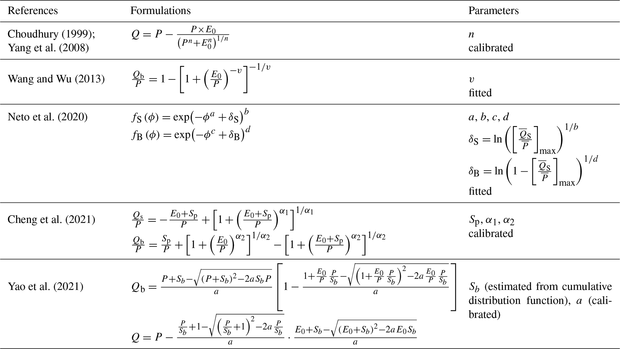
Recently, utilizing the extended Budyko framework to estimate Q_b and Q_s has attracted attention. Wang and Wu (2013) and Neto et al. (2020) established the regression relationship between baseflow fraction (BFC, the ratio of Q_b to precipitation (P)) and aridity index (ϕ, the ratio of mean annual potential evapotranspiration (E₀) to P) using analytical formulation. However, Gnann et al. (2019) reported that using only the ϕ struggles to delineate baseflow variability in humid catchments, where the impact of soil water storage capacity (S_p) is as critical as that of the ϕ. Thus, Cheng et al. (2021) proposed an analytical curve for describing mean annual Q_b by introducing S_p as another theoretical boundary. Results show that the developed curve agrees well with the observed BFC (R²= 0.75, RMSE = 0.058) and Q_b (R²=0.86, RMSE = 0.19 mm), outperforming the original Budyko framework. Analogously, Yao et al. (2021) derived similar functions incorporated the ϕ, S_p and a shape parameter to model BFC and baseflow index (BFI, the ratio of Q_b to Q). These extended Budyko frameworks accounting for S_p have advantages in simulating Q_b. However, S_p is challenging to obtain through observations and often requires calibration (Cheng et al., 2021) or computation (Yao et al., 2021), adding certain uncertainties to the model. Notably, the calibration performance of Q_s in Eq. (1) to obtain W_p (the proxy of S_p) in the catchments of China are not always satisfactory, especially in the northern catchments. Moreover, the complicated forms can bring inherent uncertainties and these studies have not validated the formulations of Q_s, which are derived by subtracting Q_b from Q or fitting curves (Cheng et al., 2021; Neto et al., 2020), implying that they may overlook the physical processes represented by surface flow. In the subsequent discussion, the Budyko framework and extended Budyko equations are collectively referred to as the “Budyko-type formulations” (Table 1).

Many researchers have observed similar behavior of Q_b to Q (Cheng et al., 2021; Gnann et al., 2019; Wang and Wu, 2013). Is there a similar behavior for Q_s? In a two-stage partitioning theory (L'vovich, 1979), runoff components are delineated based on the available water at each stage. Therefore, is there a general framework to unify different runoff components? Although various functional forms have been proposed for estimating runoff components in the literature, a universal method that reveals the mechanisms of mean annual runoff components generation and subsequent quantification and attribution is still in need.

Note that P is the mean annual precipitation, E₀ is the mean annual potential evapotranspiration, f_S(ϕ) and f_B(ϕ) are the surface flow and baseflow function, respectively and S_p is the catchment storage capacity.

To address these questions, we derived a modified two-stage partitioning framework through observational data analysis and theoretical derivation based on the Ponce-Shetty model (Ponce and Shetty, 1995; Sivapalan et al., 2011) (namely the modified Ponce-Shetty model, MPS model) at mean annual time scale. The Ponce-Shetty model is a conceptual model with physical constraint developed at annual scale to depict how precipitation is partitioned, stored and released in the catchment (Gnann et al., 2019). It posits that annual precipitation is partitioned into Q_s and soil wetting (W) and, subsequently, the resulting W is partitioned into Q_b and vaporization (V) (Sivapalan et al., 2011). The MPS model enables large-sample catchments research, which may lead to new understanding of mean annual water balance and allocation.

In general, the objectives of this study are to (1) develop a general and concise formulation to describe runoff components variability at mean annual time scale; (2) validate and compare the performance of the developed formulation against Budyko-type formulations; (3) attribute the variations of runoff components induced by the changes of precipitation and other factors. Here, we modify the Ponce-Shetty model according to some conditions and hypothesize a general runoff components model (the MPS model), that describes Q_s, Q_b and Q as a function of respective available water with one parameter. The MPS model is then validated over 662 catchments across China and the contiguous United States (the CONUS) over a wide range of hydro-meteorological circumstances. The performance of the MPS model is also compared with the Budyko-type formulations. Section 2 introduces the derivation of the MPS model. Section 3 provides the study catchments, data and the parameter estimation technique. Section 4 shows the results followed by a discussion in Sect. 5. The conclusions are summarized in Sect. 6.

2 Derivation of the Modified Ponce-Shetty Model

L'vovich (1979) proposed a conceptual theory for the two-stage catchment water balance partition at the annual time scale according to Horton's approach (Horton, 1933). Firstly, precipitation is partitioned into surface flow (Q_s) and catchment wetting (W, stored water), and then, the catchment wetting is partitioned into baseflow (Q_b) and vaporization (V, including interception loss, evaporation and transpiration). Ponce and Shetty (1995) conceptualized the partition of each step as the form of a competition, and derived the formulations of runoff components based on the proportionality hypothesis. Sivapalan et al. (2011) reintroduced the Ponce-Shetty equations as follows:

In the first stage, $P=Q_{\mathrm{s}}+W$:

$$\begin{array}{}\text{(1)}& {\displaystyle }{Q}_{\mathrm{s}}=\left\{\begin{array}{ll}\mathrm{0},& \mathrm{if}P\le {\mathit{\lambda }}_{\mathrm{s}}{W}_{\mathrm{p}}\\ \frac{{\left(P-{\mathit{\lambda }}_{\mathrm{s}}{W}_{\mathrm{p}}\right)}^{\mathrm{2}}}{P+\left(\mathrm{1}-\mathrm{2}{\mathit{\lambda }}_{\mathrm{s}}\right)W_{\mathrm{p}}},& \mathrm{if}P>{\mathit{\lambda }}_{\mathrm{s}}{W}_{\mathrm{p}}\end{array}\right.\text{(2)}& {\displaystyle }W=\left\{\begin{array}{ll}P,& \mathrm{if}P\le {\mathit{\lambda }}_{\mathrm{s}}{W}_{\mathrm{p}}\\ P-\frac{{\left(P-{\mathit{\lambda }}_{\mathrm{s}}{W}_{\mathrm{p}}\right)}^{\mathrm{2}}}{P+\left(\mathrm{1}-\mathrm{2}{\mathit{\lambda }}_{\mathrm{s}}\right)W_{\mathrm{p}}},& \mathrm{if}P>{\mathit{\lambda }}_{\mathrm{s}}{W}_{\mathrm{p}}\end{array}\right.\text{(3)}& {\displaystyle }P\to \mathrm{\infty },Q_{\mathrm{s}}\to P-W_{\mathrm{p}},W\to W_{\mathrm{p}}\end{array}$$

In the second stage, $W=Q_{\mathrm{b}}+V$:

$$\begin{array}{}\text{(4)}& {\displaystyle }{Q}_{\mathrm{b}}=\left\{\begin{array}{ll}\mathrm{0},& \mathrm{if}W\le {\mathit{\lambda }}_{\mathrm{b}}{V}_{\mathrm{p}}\\ \frac{{\left(W-{\mathit{\lambda }}_{\mathrm{b}}{V}_{\mathrm{p}}\right)}^{\mathrm{2}}}{W+\left(\mathrm{1}-\mathrm{2}{\mathit{\lambda }}_{\mathrm{b}}\right)V_{\mathrm{p}}},& \mathrm{if}W>{\mathit{\lambda }}_{\mathrm{b}}{V}_{\mathrm{p}}\end{array}\right.\text{(5)}& {\displaystyle }V=\left\{\begin{array}{ll}W,& \mathrm{if}W\le {\mathit{\lambda }}_{\mathrm{b}}{V}_{\mathrm{p}}\\ W-\frac{{\left(W-{\mathit{\lambda }}_{\mathrm{b}}{V}_{\mathrm{p}}\right)}^{\mathrm{2}}}{W+\left(\mathrm{1}-\mathrm{2}{\mathit{\lambda }}_{\mathrm{b}}\right)V_{\mathrm{p}}},& \mathrm{if}W>{\mathit{\lambda }}_{\mathrm{b}}{V}_{\mathrm{p}}\end{array}\right.\text{(6)}& {\displaystyle }W\to \mathrm{\infty },Q_{\mathrm{b}}\to W-V_{\mathrm{p}},V\to V_{\mathrm{p}}\end{array}$$

where λ_s and λ_b are the surface flow and baseflow initial abstraction coefficients, respectively, which range from 0 to 1. The larger value of λ, the more difficult it is to generate flow. W_p and V_p are catchment wetting potential and vaporization potential, respectively, which are greater than 0. The terms relative λ_sW_p and λ_bV_p are the surface flow and baseflow generation thresholds, respectively.

Note that the interannual water storage change is supposed to be negligible (Ponce and Shetty, 1995). In a companion paper of Sivapalan et al. (2011), Harman et al. (2011) employed the annual Ponce-Shetty model at mean annual time scale and validated its applicability. Using the first phase as an example, Q_s can be considered a function of λ_s, denoted as f(λ_s):

$$\begin{array}{}\text{(7)}& f\left({\mathit{\lambda }}_{\mathrm{s}}\right)=\left\{\begin{array}{ll}\mathrm{0},& \mathrm{if}{\mathit{\lambda }}_{\mathrm{s}}\ge P/W_{\mathrm{p}}\\ \frac{{\left(P-{\mathit{\lambda }}_{\mathrm{s}}{W}_{\mathrm{p}}\right)}^{\mathrm{2}}}{P+\left(\mathrm{1}-\mathrm{2}{\mathit{\lambda }}_{\mathrm{s}}\right)W_{\mathrm{p}}},& \mathrm{if}{\mathit{\lambda }}_{\mathrm{s}}<P/W_{\mathrm{p}}\end{array}\right.\end{array}$$

When ${\mathit{\lambda }}_{\mathrm{s}}<P/W_{\mathrm{p}}$, the Taylor expansion of f(λ_s) at λ_s= 0 is:

$$\begin{array}{}\text{(8)}& \begin{array}{rl}f\left({\mathit{\lambda }}_{\mathrm{s}}\right)& =f\left(\mathrm{0}\right)+f^{\prime }\left(\mathrm{0}\right)\ast {\mathit{\lambda }}_{\mathrm{s}}+{\displaystyle \frac{f^{\prime \prime }\left(\mathrm{0}\right)}{\mathrm{2}\mathrm{!}}}\ast {\mathit{\lambda }}_s^{\mathrm{2}}+\mathrm{\dots }\\ & +{\displaystyle \frac{f^n\left(\mathrm{0}\right)}{n\mathrm{!}}}\cdot {\mathit{\lambda }}_s^n+\mathrm{\dots }\end{array}\end{array}$$

Hence, we have the zeroth-order approximation:

$$\begin{array}{}\text{(9)}& f\left({\mathit{\lambda }}_{\mathrm{s}}\right)\approx {\displaystyle \frac{P^{\mathrm{2}}}{P+W_{\mathrm{p}}}}\end{array}$$

When the remainder term is relatively small, an approximation equation can be used to estimate the multi-year Q_s as:

$$\begin{array}{}\text{(10)}& Q_{\mathrm{s}}={\displaystyle \frac{P^{\mathrm{2}}}{P+W_{\mathrm{p}}}}\end{array}$$

In addition, the zeroth-order approximation of Q_b can be similarly obtained as:

$$\begin{array}{}\text{(11)}& Q_{\mathrm{b}}={\displaystyle \frac{W^{\mathrm{2}}}{W+V_{\mathrm{p}}}}\end{array}$$

To evaluate the impact of the remainder term, we calculate the relative bias (δ) of runoff components for 312 catchments in China and 350 catchments in the United States using the approximate equations (Eqs. 10 and 11) and the original Ponce-Shetty equations (Eqs. 1 and 4) (data sources in Sect. 3.1). The parameters in the original Ponce-Shetty equations are calibrated using the nonlinear least squares method. The δ is calculated as:

$$\begin{array}{}\text{(12)}& \mathit{\delta }={\displaystyle \frac{\left|\stackrel{\mathrm{̃}}{Q_y}-Q_y\right|}{Q_y}}\end{array}$$

where Q_y represents runoff components estimated by the Ponce-Shetty equations, and $\stackrel{\mathrm{̃}}{Q_y}$ represents runoff components estimated by the sapproximate equations (Eqs. 10 and 11).

The spatial distribution of δ and the cumulative distribution functions (CDFs) of δ are shown in Figs. 1 and 2, respectively. As shown in Fig. 1, 77 % of the catchments have an δ of less than 5 %. The average δ for estimating Q_s is 6.5 % in China and 4.8 % in the United States, while the average δ for estimating Q_b is 7.9 % in China and 6.6 % in the United States, with larger deviations observed in arid catchments. Figure 2 indicate that the δ values for the approximate model are within acceptable limits across both China and CONUS. The relatively low 95 % threshold values, particularly for the USA datasets, suggest that the majority of predictions fall within a narrow error range, indicating robust model performance. This acceptability of δ across regions and variables highlights the approximate equations' capability to maintain prediction accuracy under varying geographical and hydrological conditions, indicating that the zeroth-order approximation is representative for the original Ponce-Shetty model.

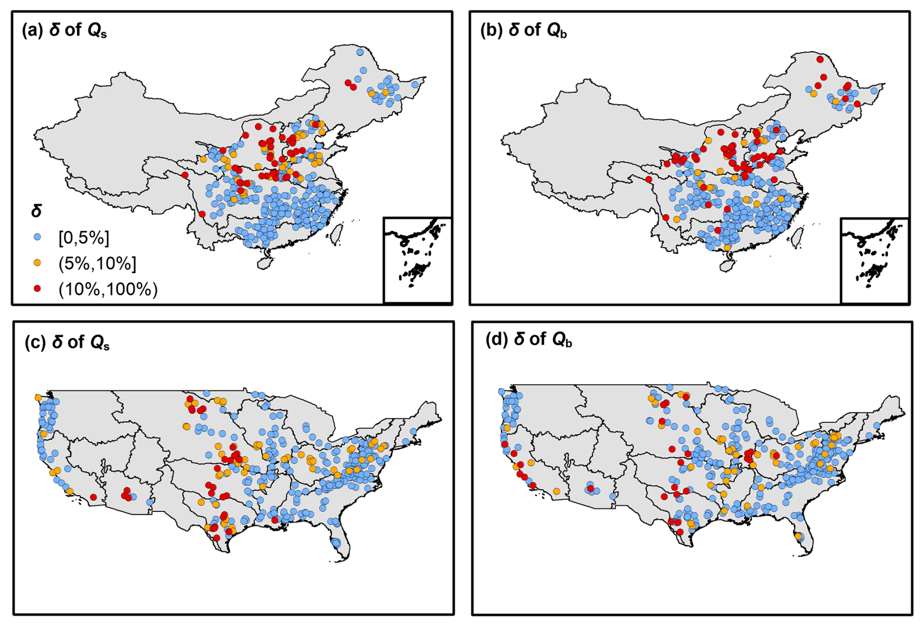
Figure 1 The distribution of relative bias (δ) between the results by the approximate equations (Eqs. 10 and 11) versus the original Ponce-Shetty equations (Eqs. 1 and 4). The first row shows the results for 312 catchments in China, and the second row shows the results for 350 catchments in CONUS. The first column corresponds to surface flow (Q_s), and the second column corresponds to baseflow (Q_b).

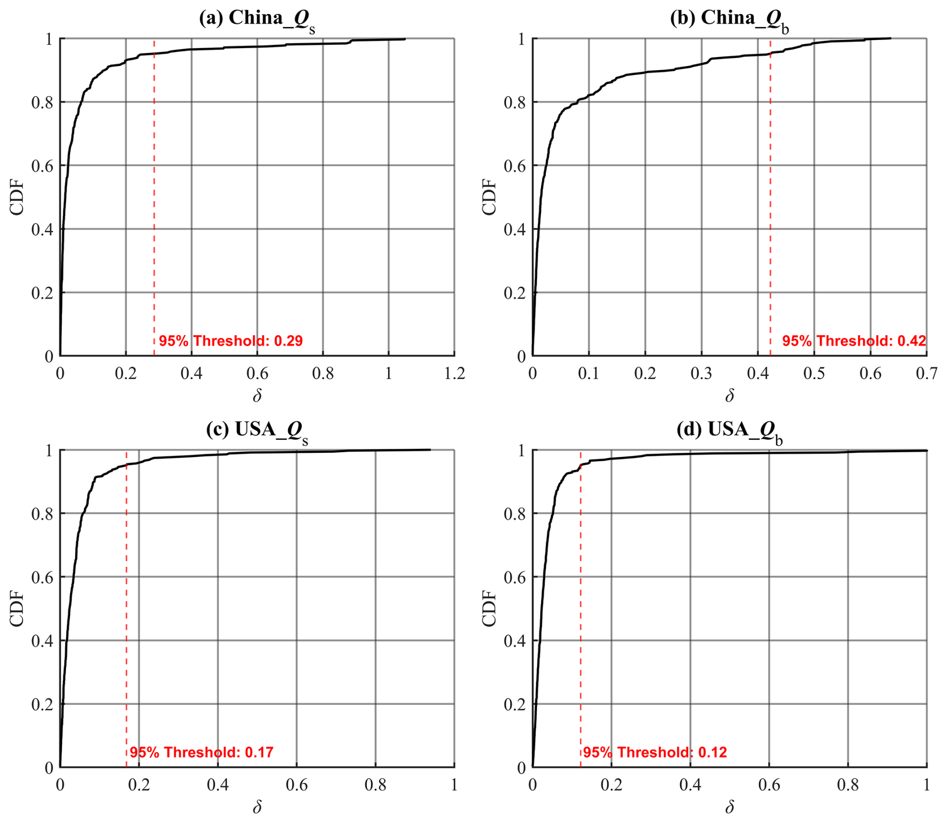
Figure 2 Cumulative distribution functions (CDFs) of the relative bias (δ) for each dataset, represented by four subplots corresponding to different regions and variables: (a) China_Q_s, (b) China_Q_b, (c) USA_Q_s, and (d) USA_Q_b. Each subplot includes a red dashed line indicating the 95 % δ threshold.

Therefore, we can approximately consider that on a multi-year scale, Q_s and Q_b can be estimated using the zeroth-order approximation in Eqs. (10) and (11). We subsequently assume a similar formulation of mean annual Q:

$$\begin{array}{}\text{(13)}& Q={\displaystyle \frac{P^{\mathrm{2}}}{P+U_{\mathrm{p}}}}\end{array}$$

where U_p is the parameter representing the upper limit of the portion remaining after precipitation is allocated to runoff, hereafter we refer to U_p as evapotranspiration potential.

Integrating Eqs. (10), (11) and (13), we conclude a general formulation to depict multi-year variability of runoff components and their quantification, hereafter referred to as the modified Ponce-Shetty model (the MPS model):

$$\begin{array}{}\text{(14)}& Q_y={\displaystyle \frac{X^{\mathrm{2}}}{X+M}}\end{array}$$

where Q_y represents runoff components (i.e., Q, Q_s, Q_b), X corresponds to the available water of each runoff component, i.e., P is the available water of Q and Q_s, and W the available water of Q_b. M is an integrated parameter, representing the comprehensive effects of catchment characteristics and atmospheric water and energy demand.

The MPS model encodes runoff components as a function of available water with only one parameter, which not only considers processes of runoff generation with physical constraints, but also, compared to the Budyko-type formulations and the original Ponce-Shetty model, is more concise in form and requires fewer parameters. Therefore, it is possible to estimate the long-term runoff components when only long-term variables are known.

3 Data and Methodology

3.1 Data

To validate the reliability of the MPS model, daily hydrological and meteorological data from 312 catchments in China (Li et al., 2024) and 350 catchments in the CONUS are collected. The criteria for catchments screening can refer to He et al. (2025). The location of all the catchments hydrological stations is shown in Fig. 3.

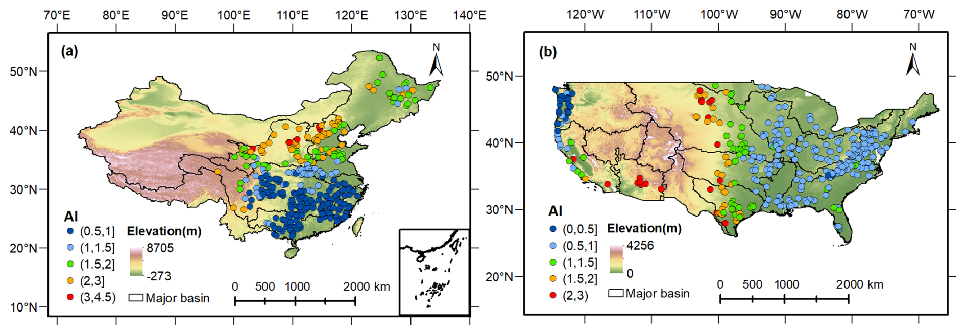
Figure 3 Location of hydrological stations for the (a) 312 catchments in China and (b) 350 catchments in the CONUS, colored by the value of aridity index (ϕ, namely $E_{\mathrm{0}}/P$).

In China, precipitation data at 0.25° spatial resolution are obtained from the China Gauge-based Daily Precipitation Analysis (CGDPA) (Shen and Xiong, 2016). Other meteorological data, including wind speed, sunshine hours, relative humidity, and air temperature, are from about 736 stations of the China Meteorological Data Service Center (http://data.cma.cn/en, last access: 11 November 2023). The in-site meteorological data are interpolated into a 10 km grid using the inverse-distance weighted method (Yang et al., 2014). We use the Penman equation (Penman, 1948) to estimate E₀ of each grid using standard meteorological inputs (e.g., radiation, humidity, wind, temperature). The Penman equation is widely recommended to estimate E₀ at catchment scale due to its physical basis (Pimentel et al., 2023; Wang et al., 2025), and it provides a consistent reference for our annual, large-sample analyses. The aridity index ϕ is subsequently calculated as $E_{\mathrm{0}}/P$. All grid data are aggregated and lumped for individual catchments. The discharge data are collected from the Hydrological Bureau of the Ministry of Water Resources of China (http://www.mwr.gov.cn/english/, last access: 20 December 2023) and are selected based on the length of records exceeding 35 years with less than 5 % missing data. The time range for all data is 1960–2000.

In the CONUS, we use data set from CAMELS (Addor et al., 2017; Newman et al., 2015). The CAMELS data set provides 662 catchments with daily time series of precipitation and observed runoff along with aridity index, and most catchments contain 35 years of continuous runoff from 1980 to 2014. The criteria for excluding catchments are referred to Gnann et al. (2019), and finally 350 catchments remained.

We use the one-parameter Lyne-Hollick digital filter (Lyne and Hollick, 1979) to separate daily Q_s and Q_b from daily Q. The Lyne-Hollick method is applied forward, backward, and forward again with a filter parameter of 0.925 and has manifested to be reliable to obtain runoff components (Lee and Ajami, 2023). We use the separated Q_s and Q_b as the reference. Although there are other baseflow separation algorithms, according to Troch et al. (2009), the choice of baseflow separation algorithm is not a significant determinant of the water balance at the annual scale.

All the hydrological and meteorological data are aggregated to the annual and mean annual time scales for further analysis.

3.2 Calibration and Validation

Spatially, to verify the MPS model's ability to characterize the variability of runoff components between catchments, we utilize the least squares fitting algorithm to estimate parameters, i.e., W_p, V_p and U_p. The three parameters are restricted to being between 0 and 50 000 mm, which is considered high enough to not affect the parameter estimation (Gnann et al., 2019).

In terms of time, we split all data into two periods for parameter calibration and validation of Eq. (14) for individual catchments. In China, the data ranges from 1960 to 2000, so we use the first 31 years (1960–1990) as the calibration period and the remaining 5–10 years (1991–2000) as the validation period. In the CONUS, the calibration period is chosen as 1980–2000, and the validation period is from 2001 to 2014. When we know mean annual Q_s, Q_b, Q, P and W of the first period, the parameters, i.e., W_p, V_p and U_p, can be derived from Eq. (14). Postulating the parameters remain unchanged during two periods, we consequently can estimate the mean annual Q_s, Q_b and Q of the second period using Eq. (14). Note that the catchment wetting W is calculated as the difference of the P and estimated Q_s.

The surface flow fraction (SFC, the ratio of surface flow to precipitation) and baseflow fraction (BFC, the ratio of baseflow to precipitation) represent the proportion of rainfall becoming different runoff components, which are commonly used to quantity surface flow and baseflow (Wang and Wu, 2013). Therefore, we evaluate the simulation of SFC and BFC as well as the volume of runoff components.

The performance of the MPS model is evaluated by the coefficient of determination (R²) and the root mean square error (RMSE):

$$\begin{array}{}\text{(15)}& {\displaystyle }{R}^{\mathrm{2}}={\left({\displaystyle \frac{{\sum }_{i=\mathrm{1}}^N\left(X_{\mathrm{sim},i}-{\stackrel{\mathrm{‾}}{X}}_{\mathrm{sim}}\right)\left(X_{\mathrm{obs},i}-{\stackrel{\mathrm{‾}}{X}}_{\mathrm{obs}}\right)}{\sqrt{{\sum }_{i=\mathrm{1}}^N{\left(X_{\mathrm{sim},i}-{\stackrel{\mathrm{‾}}{X}}_{\mathrm{sim}}\right)}^{\mathrm{2}}{\sum }_{i=\mathrm{1}}^N{\left(X_{\mathrm{obs},i}-{\stackrel{\mathrm{‾}}{X}}_{\mathrm{obs}}\right)}^{\mathrm{2}}}}}\right)}^{\mathrm{2}}\text{(16)}& {\displaystyle }\mathrm{RMSE}=\sqrt{{\displaystyle \frac{\mathrm{1}}{N}}{\sum }_{i=\mathrm{1}}^N{\left(X_{\mathrm{sim},i}-X_{\mathrm{obs},i}\right)}^{\mathrm{2}}}\end{array}$$

where X represents the evaluated variable, i.e., mean annual Q, Q_s and Q_b, SFC and BFC in this study. The subscript obs and sim represent the observed and simulated value, respectively. Higher R² and lower RMSE indicate good model performance.

3.3 Attribution Analysis

We split the data into the first period (1960–1990 in China and 1980–2000 in the CONUS) and the second period (1991–2000 in China and 2001–2014 in the CONUS) to attribute runoff components variation between two periods. Note that the attribution of ΔQ is only conducted in China because the E₀ in CAMELS dataset is a constant in each catchment. In the MPS model, we consider that the runoff changes between two long-term periods are caused by available water and other environmental and anthropogenic factors (such as land cover/use change and evapotranspiration variation) encoded by parameters. For the changes of surface flow (ΔQ_s) and total runoff (ΔQ), postulating that each variable is independent in the MPS model, the first-order approximation of the ΔQ_s and ΔQ from the second period to the first period can be expressed as (Milly and Dunne, 2002):

$$\begin{array}{}\text{(17a)}& {\displaystyle }\mathrm{\Delta }{Q}_{\mathrm{s}}={\displaystyle \frac{\partial Q_{\mathrm{s}}}{\partial P}}\mathrm{\Delta }P+{\displaystyle \frac{\partial Q_{\mathrm{s}}}{\partial W_{\mathrm{p}}}}\mathrm{\Delta }{W}_{\mathrm{p}}\text{(17b)}& {\displaystyle }\mathrm{\Delta }Q={\displaystyle \frac{\partial Q}{\partial P}}\mathrm{\Delta }P+{\displaystyle \frac{\partial Q}{\partial U_{\mathrm{p}}}}\mathrm{\Delta }{U}_{\mathrm{p}}\end{array}$$

where the two terms on the right side of Eq. (17a) respectively represent changes in Q_s caused by changes in P (ΔQ_s−P) and other factors ($\mathrm{\Delta }{Q}_{\mathrm{s}-W_{\mathrm{p}}}$), and the two terms on the right side of Eq. (17b) respectively represent changes in Q caused by changes in P (ΔQ_P) and other factors ($\mathrm{\Delta }{Q}_{W_{\mathrm{p}}}$). For convenience, we refer partial derivative coefficient $\frac{\partial Q_{\mathrm{s}}}{\partial P}$, $\frac{\partial Q_{\mathrm{s}}}{\partial W_{\mathrm{p}}}$, $\frac{\partial Q}{\partial P}$ and $\frac{\partial Q}{\partial U_{\mathrm{p}}}$ in Eq. (17) as ζ_Qs−P, ${\mathit{\zeta }}_{Q\mathrm{s}-W_{\mathrm{p}}}$, ζ_Q−P and ${\mathit{\zeta }}_{Q-W_{\mathrm{p}}}$, which can be calculated as:

$$\begin{array}{}\text{(18a)}& {\displaystyle }{\mathit{\zeta }}_{Q\mathrm{s}-P}={\displaystyle \frac{P^{\mathrm{2}}+\mathrm{2}P{W}_{\mathrm{p}}}{{\left(P+W_{\mathrm{p}}\right)}^{\mathrm{2}}}}\text{(18b)}& {\displaystyle }{\mathit{\zeta }}_{Q\mathrm{s}-W_{\mathrm{p}}}={\displaystyle \frac{-P^{\mathrm{2}}}{{\left(P+W_{\mathrm{p}}\right)}^{\mathrm{2}}}}\text{(18c)}& {\displaystyle }{\mathit{\zeta }}_{Q-P}={\displaystyle \frac{P^{\mathrm{2}}+\mathrm{2}P{U}_{\mathrm{p}}}{{\left(P+U_{\mathrm{p}}\right)}^{\mathrm{2}}}}\text{(18d)}& {\displaystyle }{\mathit{\zeta }}_{Q-W_{\mathrm{p}}}={\displaystyle \frac{-P^{\mathrm{2}}}{{\left(P+U_{\mathrm{p}}\right)}^{\mathrm{2}}}}\end{array}$$

The changes of baseflow (ΔQ_b) is induced by the variations of the W and V_p. However, we focus more on the impact of P in application. Therefore, we combine Eqs. (10), (11) and $W=P-Q_{\mathrm{s}}$, so the Q_b can be calculated as :

$$\begin{array}{}\text{(19)}& Q_{\mathrm{b}}={\displaystyle \frac{P^{\mathrm{2}}{W}_{\mathrm{p}}^{\mathrm{2}}}{\left(P+W_{\mathrm{p}}\right)\left(P{W}_{\mathrm{p}}+P{V}_{\mathrm{p}}+W_{\mathrm{p}}{V}_{\mathrm{p}}\right)}}\end{array}$$

The ΔQ_b can be attributed as the variations of P, W_p and V_p:

$$\begin{array}{}\text{(20)}& \mathrm{\Delta }{Q}_{\mathrm{b}}={\displaystyle \frac{\partial Q_{\mathrm{b}}}{\partial P}}\mathrm{\Delta }P+{\displaystyle \frac{\partial Q_{\mathrm{b}}}{\partial W_{\mathrm{p}}}}\mathrm{\Delta }{W}_{\mathrm{p}}+{\displaystyle \frac{\partial Q_{\mathrm{b}}}{\partial V_{\mathrm{p}}}}\mathrm{\Delta }{V}_{\mathrm{p}}\end{array}$$

where the three terms on the right side of Eq. (20) respectively represent changes in Q_b caused by changes in P (ΔQ_b−P), W_p ($\mathrm{\Delta }{Q}_{\mathrm{b}-{\mathrm{W}}_{\mathrm{p}}}$) and V_p ($\mathrm{\Delta }{Q}_{\mathrm{b}-{\mathrm{V}}_{\mathrm{p}}}$). The partial derivative coefficient $\frac{\partial Q_{\mathrm{b}}}{\partial P}$ (${\mathit{\zeta }}_{Q_{\mathrm{b}}-P}$), $\frac{\partial Q_{\mathrm{b}}}{\partial W_{\mathrm{p}}}$ (${\mathit{\zeta }}_{Q_{\mathrm{b}}-W_{\mathrm{p}}}$) and $\frac{\partial Q_{\mathrm{b}}}{\partial V_{\mathrm{p}}}$ (${\mathit{\zeta }}_{Q_{\mathrm{b}}-V_{\mathrm{p}}}$) can be calculated as:

$$\begin{array}{}\text{(21a)}& {\displaystyle }{\mathit{\zeta }}_{Q_{\mathrm{b}}-P}={\displaystyle \frac{\mathrm{2}{P}^{\mathrm{2}}{W}_{\mathrm{P}}^{\mathrm{3}}{V}_{\mathrm{p}}+P^{\mathrm{2}}{W}_{\mathrm{P}}^{\mathrm{4}}+\mathrm{2}P{W}_{\mathrm{P}}^{\mathrm{4}}{V}_{\mathrm{p}}}{{\left(P+W_{\mathrm{p}}\right)}^{\mathrm{2}}{\left(P{W}_{\mathrm{p}}+P{V}_{\mathrm{p}}+W_{\mathrm{p}}{V}_{\mathrm{p}}\right)}^{\mathrm{2}}}}\text{(21b)}& {\displaystyle }{\mathit{\zeta }}_{Q_{\mathrm{b}}-W_{\mathrm{p}}}={\displaystyle \frac{P^{\mathrm{4}}{W}_{\mathrm{P}}^{\mathrm{2}}+\mathrm{2}{P}^{\mathrm{4}}{W}_{\mathrm{p}}{V}_{\mathrm{p}}+\mathrm{2}{P}^{\mathrm{3}}{W}_{\mathrm{P}}^{\mathrm{2}}{V}_{\mathrm{p}}}{{\left(P+W_{\mathrm{p}}\right)}^{\mathrm{2}}{\left(P{W}_{\mathrm{p}}+P{V}_{\mathrm{p}}+W_{\mathrm{p}}{V}_{\mathrm{p}}\right)}^{\mathrm{2}}}}\text{(21c)}& {\displaystyle }{\mathit{\zeta }}_{Q_{\mathrm{b}}-V_{\mathrm{p}}}={\displaystyle \frac{-P^{\mathrm{2}}{W}_{\mathrm{P}}^{\mathrm{2}}}{{\left(P+W_{\mathrm{p}}\right)}^{\mathrm{2}}{\left(P{W}_{\mathrm{p}}+P{V}_{\mathrm{p}}+W_{\mathrm{p}}{V}_{\mathrm{p}}\right)}^{\mathrm{2}}}}\end{array}$$

To verify the applicability of the MPS model for runoff components attribution, we compare the calculated ΔQ_s, ΔQ_b and ΔQ using Eqs. (17) and (20) with the observed ΔQ_s, ΔQ_b and ΔQ between two periods. The evaluation metrics are R² and RMSE.

The relative contribution ratios of P and other factors to runoff components change are calculated as:

$$\begin{array}{}\text{(22a)}& {\displaystyle }{\mathit{\eta }}_P={\displaystyle \frac{\mathrm{\Delta }{Q}_{y-P}}{\mathrm{|}\mathrm{\Delta }{Q}_{y-P}\mathrm{|}+\mathrm{|}\mathrm{\Delta }{Q}_{y-W_{\mathrm{p}}}\mathrm{|}+\mathrm{|}\mathrm{\Delta }{Q}_{y-V_{\mathrm{p}}}\mathrm{|}}}\times \mathrm{100}\mathit{\%}\text{(22b)}& {\displaystyle }{\mathit{\eta }}_{W_{\mathrm{p}}}={\displaystyle \frac{\mathrm{\Delta }{Q}_{y-W_{\mathrm{p}}}}{\mathrm{|}\mathrm{\Delta }{Q}_{y-P}\mathrm{|}+\mathrm{|}\mathrm{\Delta }{Q}_{y-W_{\mathrm{p}}}\mathrm{|}+\mathrm{|}\mathrm{\Delta }{Q}_{y-V_{\mathrm{p}}}\mathrm{|}}}\times \mathrm{100}\mathit{\%}\text{(22c)}& {\displaystyle }{\mathit{\eta }}_{V_{\mathrm{p}}}={\displaystyle \frac{\mathrm{\Delta }{Q}_{y-V_{\mathrm{p}}}}{\mathrm{|}\mathrm{\Delta }{Q}_{y-P}\mathrm{|}+\mathrm{|}\mathrm{\Delta }{Q}_{y-W_{\mathrm{p}}}\mathrm{|}+\mathrm{|}\mathrm{\Delta }{Q}_{y-V_{\mathrm{p}}}\mathrm{|}}}\times \mathrm{100}\mathrm{\%}\end{array}$$

where η_P, ${\mathit{\eta }}_{W_{\mathrm{p}}}$ and ${\mathit{\eta }}_{V_{\mathrm{p}}}$ are the relative contribution ratios of P, W_p and V_p to runoff components, respectively. We subsequently use the absolute values of η to identify the dominant factor impacting runoff components.

4 Results

4.1 Inter-Catchment Variability of Runoff Components

We employ the MPS model to fit the relationship between mean annual available water and runoff components. In China, as shown in Fig. 4a–c, the MPS model performs well in describing runoff components variability between catchments, with R² values of 0.86, 0.69 and 0.91 for fitting Q_s, Q_b and Q, respectively. The solid lines are the best-fitted MPS curves derived using the least squares fitting algorithm, implying the median values of different parameters. We also give the potential upper and lower limits of W_p, V_p and U_p across catchments. Similarly, Fig. 4d–f illustrates that the MPS model achieves good fitting in the CONUS, with R² of 0.81, 0.44 and 0.80 for fitting Q_s, Q_b and Q, respectively. The fitted parameters in the CONUS are smaller than those in China, while they have more comprehensive ranges between catchments, meaning a more significant heterogeneity in climate and underlying surface.

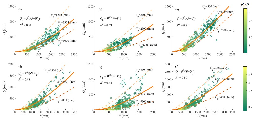
Figure 4 The MPS model relating (a) P versus Q_s, (b) W versus Q_b and (c) P versus Q in China and (d) P versus Q_s, (e) W versus Q_b and (f) P versus Q in the CONUS. The lines are the fitted MPS curves with best fitting (solid line) and potential upper limit and lower limit (dashed lines) parameters.

Figure 4 demonstrates that the MPS model can effectively reproduce the spatial variability of different runoff components along with the aridity index ($E_{\mathrm{0}}/P$), which are primarily controlled by the available water of the corresponding partition stage. The performance of MPS model to fit Q_s and Q is better than that of Q_b, indicating that the factors controlling Q_b are more complicated and not fully reflected in the model. With catchment properties and other factors (integrated by the parameters in the MPS model) remaining unchanged, the more the available water, the higher the runoff generated. Conversely, smaller parameter values are associated with greater runoff for a given amount of available water.

4.2 Validation of Runoff Components Estimation

Figure 5 shows the estimated mean annual Q_s, Q_b and Q in validation periods using the MPS model with inverted parameters in Eq. (14) in China and the CONUS. The simulated runoff components match very well with the observed, with R² greater than 0.97 and RMSE less than 66 mm. There is no significant difference in the performance in simulating Q_s, Q_b, and Q, except for a slight underestimation in simulating Q_b of catchments in China and some in the CONUS.

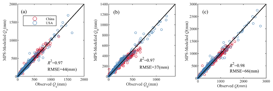
Figure 5 The observed and simulated mean annual (a) surface flow, (b) baseflow and (c) total runoff by the MPS model in China (red circles) and the CONUS (blue circles).

In panels (a), (b), and (c), we observe that the scatter points for both China (red circles) and the CONUS (blue circles) are closely aligned with the 1:1 line, further underscoring the strong correlation between modeled and observed values. Specifically, the results show that the MPS model effectively captures surface flow (Q_s), baseflow (Q_b), and total runoff (Q) for both regions. Despite the generally good performance, a slight underestimation of Q_b is evident in a subset of catchments in China and, to a lesser extent, in the CONUS. However, these discrepancies are minimal and do not significantly detract from the model's overall accuracy.

Figure 6 presents the estimation of SFC and BFC in validation periods using the MPS model. Similar to the simulation of Q_s, the two methods also show highly consistent estimation of SFC (panel (a)), with R² of 0.94 and RMSE of 0.03. This demonstrates the MPS model's robust capability to estimate the surface flow fraction in China and the CONUS, closely aligning with the observed data. Panel (b) presents the estimation of BFC, where the MPS model achieves significant accuracy, reflected by the same R² and RMSE values (0.94 and 0.03, respectively). This strong performance indicates that the MPS model is highly effective in simulating SFC and BFC across various catchments.

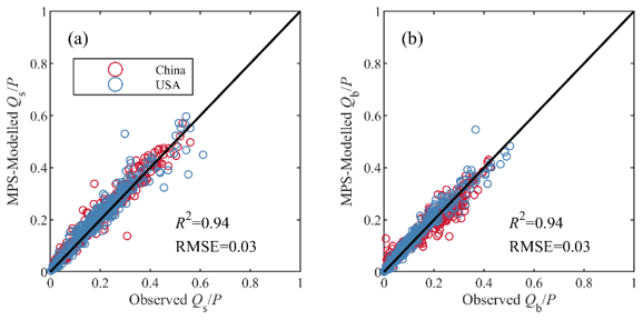
Figure 6 The observed and simulated (a) surface flow fraction ($Q_{\mathrm{s}}/P$) and (b) baseflow fraction ($Q_{\mathrm{b}}/P$) by the MPS model in China (red circles) and the CONUS (blue circles).

Figures 5 and 6 document that the MPS model can effectively estimate the multi-year average of all runoff components and the proportions of precipitation allocated to runoff.

The good validation performance of the MPS model verified our hypothesis that the parameters in the general formulations remain stable at the mean annual time scale. The parameters reflect the comprehensive impact of climate and catchment characteristics, i.e., catchment wetting potential (W_p), vaporization potential (V_p) and the upper limit of the portion remaining after precipitation is allocated to runoff (U_p). As shown in Fig. 7a–c, the spatial distribution of the parameters across China exhibits pronounced divergence between the northern and southern catchments, as well as the eastern and the western. The W_p, V_p and U_p exhibit similar spatial patterns, which can be approximately divided into two tiers from north to south. In the catchments of the Songliao River Basin in the northeast, the Yangtze River Basin and Pearl River Basins in the south, the parameters are relatively small, with W_p and U_p ranging from 0 to 2000 mm, and V_p from 0 to 4000 mm, resulting large flow. In the catchments of the Yellow River Basin, Huaihe River Basin and Haihe River Basin in the north, the parameters are quite large and usually more than 5000 mm and even 8000 mm, leading to small flow. From west to east, W_p exhibits higher values in the Yangtze and Yellow Rivers Basin sources, whereas V_p and U_p are smaller in the source regions. This disparity may reflect variations in the two-stage partition of precipitation, contributing to spatial differences in total runoff. According to Fig. 7c, we can deduce that the spatial distribution of higher total runoff in south and lower in north across China, aligning with previous observational studies (He et al., 2021; He et al., 2022; Yang et al., 2019).

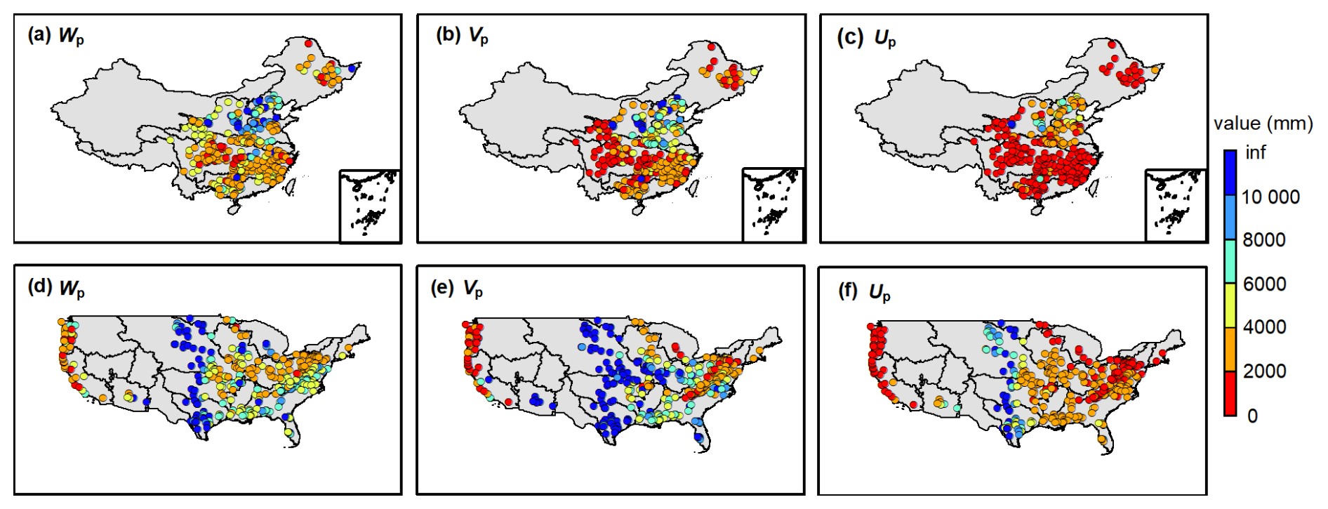
Figure 7 The (a) wetting potential (W_p), (b) vaporization potential (V_p) and (c) evapotranspiration potential (U_p) of the catchments in China and (d) wetting potential (W_p), (e) vaporization potential (V_p) and (f) evapotranspiration potential (U_p) of the catchments in the CONUS.

Figure 7d–f shows an evident west-east discrepancy of the three parameters across the CONUS. Typically, W_p, V_p and U_p of the catchments in the west coast and eastern regions are less than 5000 mm, while parameters in the central United States are extensive with values more than 8000 mm. This indicates relatively low flow in the central regions. Notably, the parameters upper limits in the catchments of the CONUS are significantly higher than those in China. The extremely large values may be associated with significant parameter uncertainty (Gnann et al., 2019). Figure 7 demonstrates that the values of the three parameters are larger in arid catchments and their spatial patterns are similar to that of climate zoning, which provides insights for parameterization.

Figure 8 shows the violin plots of the parameters in the catchments of China and the CONUS. The median values of W_p, V_p, and U_p in China are 3659, 2220 and 1453 mm, respectively. The median values of W_p, V_p, and U_p in the CONUS are 4531, 3424 and 2385 mm, respectively. Overall parameters in China are smaller and denser than those in the CONUS, implying a smaller variability of runoff components in China. Furthermore, the C_v value of V_p (1.6 in China and 6.8 in the CONUS) is the largest, followed by U_p (0.9 in China and 1.6 in the CONUS), and the smallest for W_p (0.6 in China and 1.5 in the CONUS). This indicates that the parameter dispersion controlling the second partition stage of rainfall is the greatest, which could partly account for the challenges in accurately estimating Q_b.

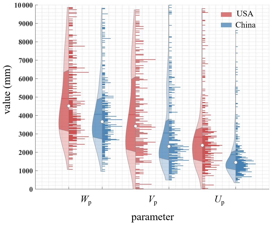
Figure 8 Violin plots of the parameters in the catchments of China and the CONUS. In each violin plot, the left side represents the distribution, with the shaded area indicating the box plot, the dot representing the mean, and the right side showing the histogram.The length of the histogram represents the number of catchments (values larger than 10 000 are not shown).

4.3 The Changes Attribution of Runoff Components

The metrics to evaluate the attribution results between the changes of the observed and simulated runoff components are shown in Table 2. We use the MPS model to estimate the changes of Q_s (ΔQ_s), Q_b (ΔQ_b) and Q(ΔQ) from two long-term periods by Eqs. (17) and (20), and for comparison, we use the Budyko framework to estimate ΔQ, which is considered as the changes induced by P, E₀, and parameter n (the calculation formulations can refer Xu et al. (2014)). The estimated and observed runoff components variations exhibit high consistency (Fig. 9), with an R² of 0.99 and RMSE of 1.6 mm of ΔQ_s attribution and R² of 0.88 and RMSE of 18 mm of ΔQ_b attribution, respectively. As for ΔQ, both the MPS model and the Budyko framework can attain satisfactory performance, while the MPS model has a higher R² (0.91) than the Budyko framework (0.89). Table 2 demonstrates that the MPS model can accurately quantify changes in runoff components over two periods. Subsequently, we quantify the contribution of precipitation and other factors (encoded by parameter W_p and V_p) to ΔQ_s and ΔQ_b.

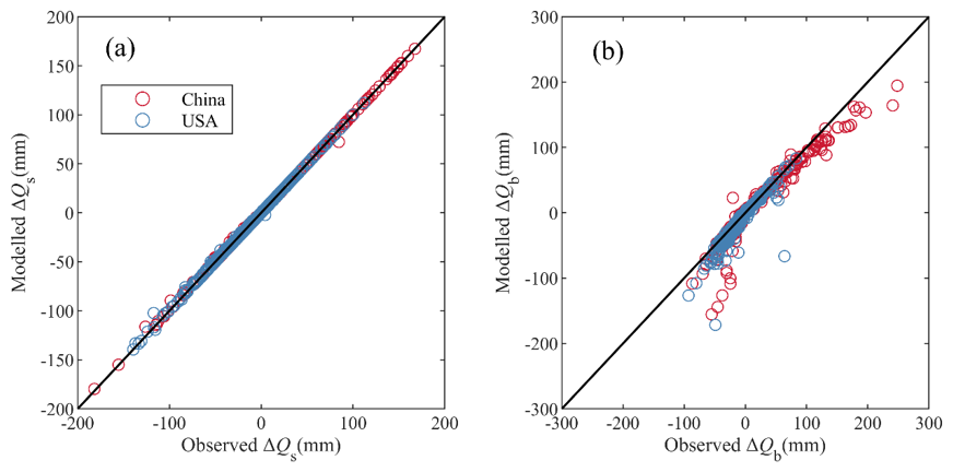
Figure 9 The observed and modelled (a) surface flow variations and (b) baseflow variations by the MPS model.

Table 2 The metrics of the attribution validation.

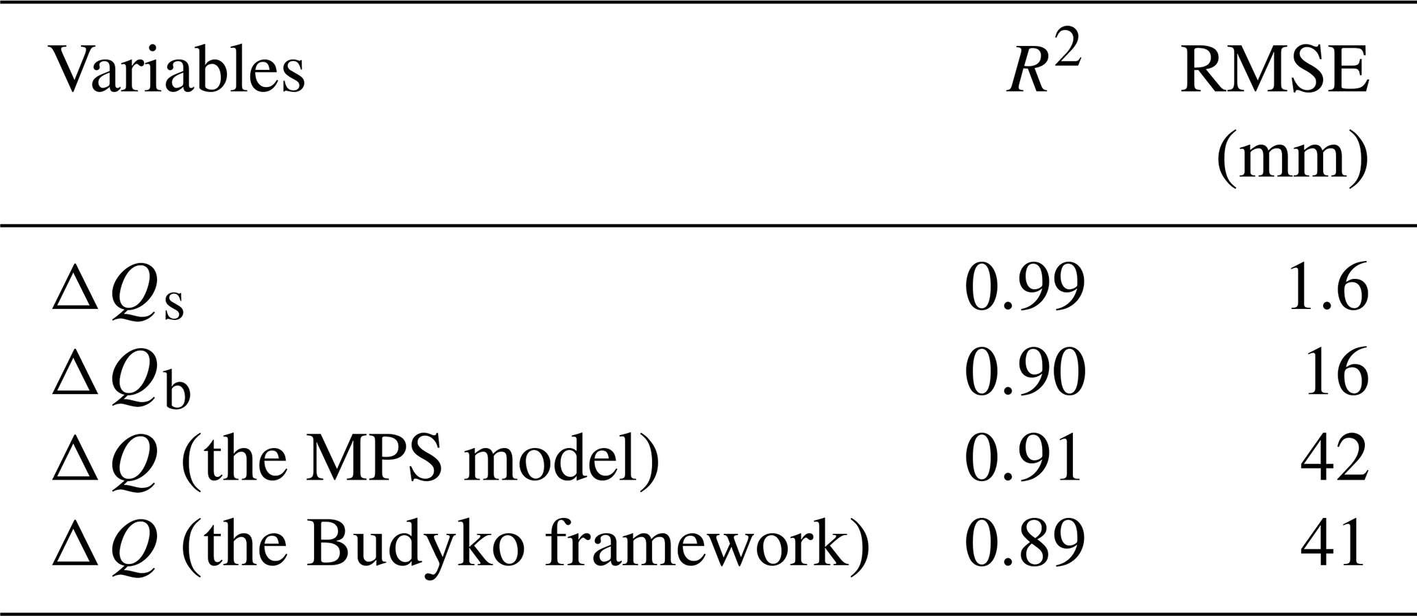
Figure 10 shows the ΔQ_s induced by P (ΔQ_s−P) and other factors ($\mathrm{\Delta }{Q}_{\mathrm{s}-W_{\mathrm{p}}}$) along with the dominant factor in the catchments of China and the CONUS. From 1960–1990 to 1991–2000 in China, the multi-year variation in P has resulted in Q_s change ranging from −105 to 344 mm, mainly increasing Q_s in the catchments of the Songliao River Basin, the middle and lower Yangtze River Basin, the Southeast River Basin and Pearl River Basin, and decreasing Q_s in the catchments of the Yellow River Basin and the upper Yangtze River Basin (Fig. 10a). The variations of other factors, such as land use/cover change and human activities, have resulted in Q_s change ranging from −186 to 124 mm, primarily decreases Q_s in 70 % catchments (Fig. 10b). P and other W_p is the dominant factor altering Q_s in southern and northern China, respectively (Fig. 10c). From 1980–2000 to 2000–2014 in the CONUS, variation in P has resulted in Q_s change ranging from −469 to 149 mm, mainly increasing Q_s in the catchments of Interior Plains (except Great Plains), Coastal Plain, Interior highlands and Appalachian Plain, and decreasing Q_s in the catchments of the Great Plains and Pacific Mountains (the physiographic divisions are referred to Wu et al. (2021)) (Fig. 10d). The variations of other factors have resulted in Q_s change ranging from −230 to 467 mm, primarily decreases Q_s in 75 % catchments (Fig. 10e). The catchments in the CONUS dominated by P and W_p account for 43 % and 57 %, respectively (Fig. 10f).

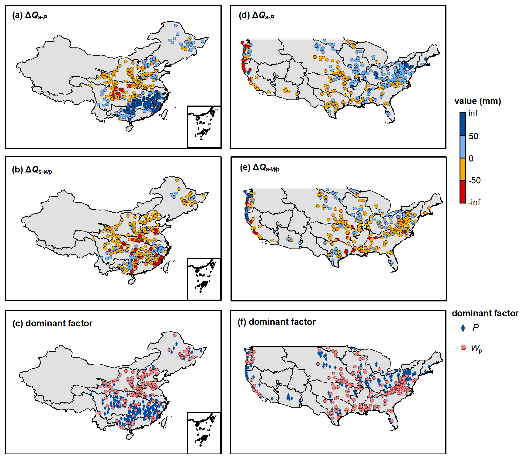
Figure 10 The surface flow change induced by precipitation and wetting potential (W_p) along with the dominant controlling factor.

Figure 11 shows the ΔQ_b induced by P (ΔQ_b−P), W_p ($\mathrm{\Delta }{Q}_{\mathrm{b}-W_{\mathrm{p}}}$) and V_p ($\mathrm{\Delta }{Q}_{\mathrm{b}-V_{\mathrm{p}}}$) in the catchments of China and the CONUS. The spatial pattern of the effect of P on Q_b is similar to that of the Q_s, resulting in Q_b change from −38 to 79 mm in China (Fig. 11a) and −129 to 92 mm in the CONUS (Fig. 11e), respectively. Catchment wetting potential has a positive effect on Q_b in 70 % and 75 % catchments of China and the CONUS, respectively (Fig. 11b and f), mainly in the northern China and the Interior Highlands, Coastal Plain and Appalachian Highlands of the CONUS. Vaporization potential has a negative effect on Q_b in 56 % and 77 % catchments of China and the CONUS, respectively, mainly in the upper Yangze River Basin and northern China and the central and southeastern CONUS (Fig. 11c and g). Although V_p is the dominant factor controlling Q_b variation in most catchments in both China (62 %) and the CONUS (71 %) (Fig. 11d and h), the contributions of the P, W_p and V_p are not significantly discrepant in terms of magnitude.

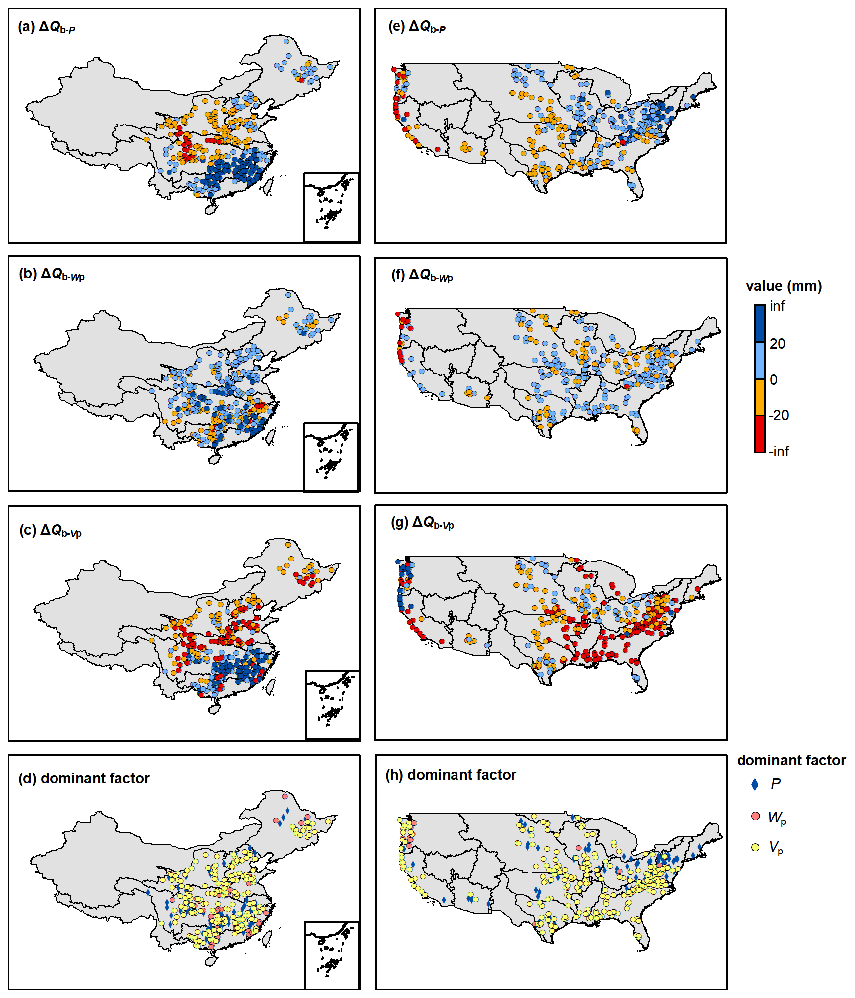
Figure 11 The baseflow change induced by precipitation, wetting potential (W_p) and vaporization potential (V_p) along with the dominant controlling factor.

Overall, Figs. 10 and 11 illustrate that the variation of Q_s is jointly controlled by P and other factors, while the variation of Q_b is mainly influenced by V_p. This demonstrates that Q_s is closely related to rainfall and soil storage capacity, while Q_b is more affected by catchment attributes, atmospheric water and energy demand, etc. In regions where runoff components are reduced, focus should be given to the risks of drought and river discontinuity; conversely, in areas experiencing runoff components increase, there is a need to guard against the risk of flooding.

5 Discussion

5.1 Superiorities of the MPS Model

The researches about long-term runoff components quantification and attribution are currently fragmented and region-specific (Beck et al., 2013; Gnann, 2021). This study has developed a general formulation (the MPS model) through observational data analysis and theoretical derivation based on the Ponce-Shetty model, unveiling the patterns of variability in different runoff components at mean annual time scale. Compared to the commonly used Budyko-type formulations, it can not only estimate mean annual Q and Q_b, but also can depict the variability of Q_s. Figure 12 shows the estimated mean annual runoff components by the Budyko-type formulations (equations in the second (Choudhury, 1999; Yang et al., 2008) and fifth (Cheng et al., 2021) rows of Table 1 in this paper). The Budyko-type formulations also achieve good validation performance, with R² greater than 0.95 and RMSE less than 78 mm. Although the MPS model and the Budyko-type formulations are comparable in terms of R², especially with almost equal simulation results of Q_s, the MPS model reduced the RMSE values by 10 and 12 mm for estimating Q_b, respectively.

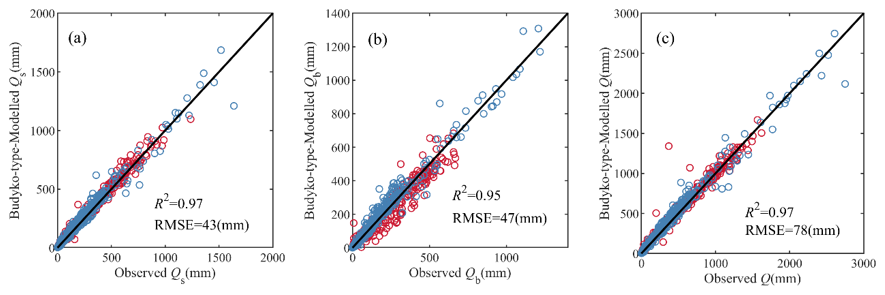
Figure 12 The observed and simulated mean annual (a) surface flow, (b) baseflow and (c) total runoff by the Budyko-type formulations in China (red circles) and the CONUS (blue circles).

Figure 13 presents the estimation of SFC and BFC in validation periods using the Budyko-type formulations. The two methods also show highly consistent estimation of SFC, with R² of 0.94 and RMSE of 0.03. However, the Budyko-type formulations underestimate the BFC of most catchments in China, while the MPS model greatly improves the simulation accuracy of BFC.

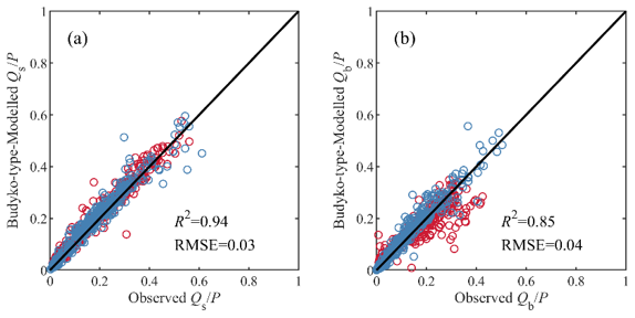
Figure 13 The observed and simulated (a) surface flow fraction ($Q_{\mathrm{s}}/P$) and (b) baseflow fraction ($Q_{\mathrm{b}}/P$) by the MPS model in China (red circles) and the CONUS (blue circles).

In conclusion, the MPS model has comparable capability in simulating Q_s and SFC to that of Budyko-type formulations. Moreover, it outperforms Budyko-type formulations in estimating Q_b and Q, and reveals superiority in estimating BFC. By characterizing runoff components as functions of available water at corresponding stages with a composite parameter, the MPS model is more concise in form and eliminates additional and complex parameter computations, thereby facilitating broader application in large-sample investigations.

In addition to precisely quantifying runoff components and the allocation of precipitation, this model has innovatively attributed the contributions of different factors on the changes of Q_s and Q_b. Our results show that the variation of Q_s is jointly controlled by P and other factors. P plays an dominant role in the variation of Q_s in the catchments of the Yangtze River Basin, Southeast Basin and Pearl River Basin of China and the west coast of the CONUS, where precipitation has been reported to have undergone significant changes (Li et al., 2021; Mallakpour and Villarini, 2017; Massoud et al., 2020; Xu et al., 2022). This is possibly due to more extreme precipitation events and summer rainfall in the middle-lower Yangtze River Basin (Ye et al., 2018) and an increasing trend in the frequency of heavy precipitation over large areas of the CONUS (Mallakpour and Villarini, 2017). Previous studies reported that the variation of Q in these regions are dominated by P (He et al., 2022; Huang et al., 2016). Now it seems that P mainly affects the first allocation stage (Q_s) and consequently change total runoff. The variation of Q_b is mainly influenced by V_p, indicating that we should pay more attention to the changes of catchment attributes, atmospheric water and energy demand in most catchments when investigating Q_b.

Overall, this conceptual model extracted from observed rainfall-runoff data provides a concise, general and effective tool for predicting runoff components, and evaluating their responses to climate and environment under global change.

5.2 Parameter Interpretation

In the MPS model, each runoff component is associated with a parameter that can be interpreted as the upper limit of the remaining portion of available water after it has been partitioned into runoff at each stage. For instance, in the first stage, precipitation is allocated to surface flow and catchment wetting, with W_p representing the upper limit of catchment wetting, which describes the catchment's storage capacity related to soil, topography and so on (Cheng et al., 2022). W_p is influenced by soil properties and available storage capacity, determining the fraction of precipitation that rapidly becomes surface runoff versus what is stored. For the second stage, the available water comes from catchment wetting, which is then allocated to baseflow and vaporization. The parameter V_p is the upper limit of the fraction of wetting returned to the atmosphere as water vapor (Ponce and Shetty, 1995), and is likely responds to subsurface characteristics such as aquifer permeability and geological layering. For instance, in highly heterogeneous aquifers with well-developed preferential pathways (e.g., fractured rock or karst systems), water is rapidly drained toward the stream, leading to a higher efficiency of baseflow production and thus a lower V_p value (as less water is retained for evaporation). Conversely, in catchments with more homogeneous, porous media (e.g., sandy aquifers), water movement is slower and more diffuse, potentially allowing for a greater fraction of stored water to be evaporated, resulting in a higher V_p. For the total runoff, we consider precipitation as the available water competing with evapotranspiration, whose upper limit is represented by the parameter U_p. Similar to V_p in the second stage, U_p can be regarded as a sort of atmospheric water and energy limit (somewhat analogous to potential evapotranspiration) and emerges from the interaction of the available energy, vegetation and other catchment characteristics. To some extent, the MPS model links Q_s and Q_b with Q using P in the first trade-off and V_p in the second trade-off, so that the forms of different runoff components can be unified.

Additionally, we compared the distribution of the parameters in the MPS model with that in Gnann et al. (2019) and Sivapalan et al. (2011), which did not omit the initial abstraction coefficients λ_s and λ_b. There is a very similar spatial pattern of W_p and V_p in the CONUS. Specifically, high W_p can be seen in the middle of the United States (Great Plains) and the east (southern parts of the Appalachians) (Fig. 7d), and high V_p can be seen in the middle of the United States (Great Plains) and all southern regions (Fig. 7e). This, to some extent, illustrates the rationality of the simplification of the original Ponce-Shetty model in describing the spatial variability of runoff components. According to Ponce and Shetty (1995) and Sivapalan et al. (2011), the products λ_sW_p and λ_bV_p are viewed as the initial abstraction to generate runoff. This definition is reasonable for short-term scales, such as event and annual scales. However, on the multi-annual scale, the catchment maintains a state of water balance and water losses can be disregarded (Han et al., 2020). Hence, simplifying λ to zero is rational to quantify and attribute runoff components and offer a new perspective on the long-term catchment water balance.

5.3 Uncertainties and Future Improvements

It is important to acknowledge several uncertainties in this study. First, the definition of “baseflow” itself introduces uncertainty. Although widely used as a collective term for delayed streamflow components, baseflow encompasses contributions from hydrologically distinct sources such as groundwater drainage, hyporehic exchange, snowmelt, and deeper subsurface leakage-each with distinct origins, timescales, and sensitivities to environmental factors. For instance, groundwater flow and deep leakage are strongly controlled by geological heterogeneity, including the distribution of rock types, porosity, permeability, faults, and fractures (Schiavo, 2023). In contrast, snowmelt baseflow, on the other hand, is mainly driven by temperature variations within interannual to decadal climate cycles.

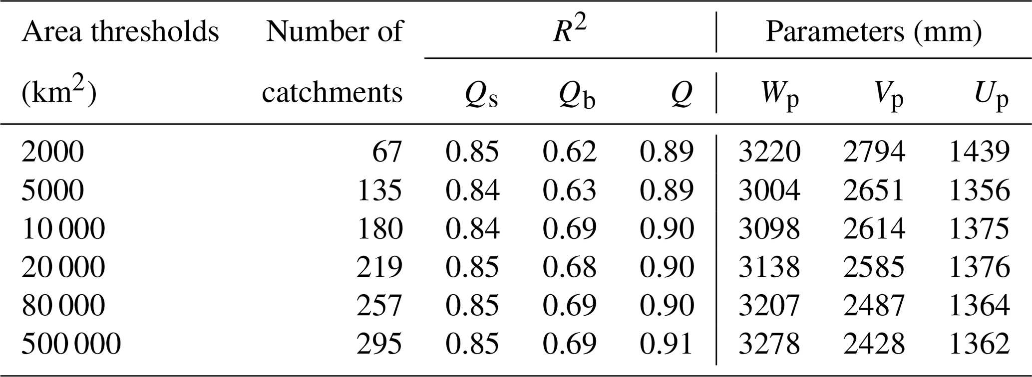
The definition of baseflow directly influences the selection of catchment areas. Guided by this macro-scale definition-viewing baseflow as the relatively stable portion of total runoff-we included large catchments in our analysis. While this inclusion may be a source of error, it does not affect the key finding that the MPS model effectively captures the variability of mean annual runoff components across catchments. A sensitivity analysis of the model's performance under different area thresholds is provided in Appendix Table A1. Future studies could combine isotope tracing with hydrological modeling to better quantify the contributions of these different sources.

Second, methodological uncertainty arises from the digital filter method (i.e., the Lyne–Hollick algorithm) for baseflow separation. While practical and widely applied, this approach is deterministic and does not explicitly account for uncertainties related to aquifer heterogeneity, such as spatial variability in hydraulic conductivity, preferential flow paths, or geologic structures. Future work could adopt stochastic frameworks such as Monte Carlo simulation by generating multiple realistic realizations of aquifer heterogeneity to obtain more robust and probabilistic baseflow estimates (Schiavo, 2023). Additionally, our study did not take into account the spatial heterogeneity of groundwater flow, particularly its preferential pathways through fractures, macropores, or highly permeable sedimentary layers. Event-scale analyses indicate that stormflow volumes and hysteresis patterns covary with subsurface connectivity and its timing. For example, Zuecco et al. (2019) used graph-theory metrics to quantify connectivity in headwater catchments and linked maximum connectivity to stormflow. While our study operates at mean-annual scales, these findings are consistent with our interpretation that geological heterogeneity and preferential pathways (fractures, karst, macropores) modulate the V_p dispersion and, in turn, the aggregate baseflow fraction. Future work could employ numerical models or distributed hydrological models that explicitly represent geological structures to better capture the effects of preferential flow paths at smaller scales.

The sensitivity of runoff to changes in climatic and environmental factors has always been highly anticipated. Schaake (1990) first introduced the concept of climate elasticity coefficients to quantify it, defined as the ratio of the relative change in mean annual runoff to the relative change in climatic factors. Various expressions have been widely applied in evaluating the hydrological response to multi-annual average climate change (Sun et al., 2014; Xu et al., 2014). The only climatic factor in the MPS model is P, so we primarily focuses on the elasticity of runoff components to P (ε), which can be expressed as ${\mathit{\epsilon }}_{y-P}=\frac{\partial Q_y}{\partial P}/\frac{Q_y}{P}$, quantifying the percentage of runoff components change caused by 1 % change in P.

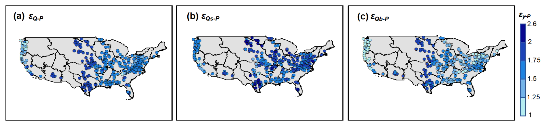
Figure 14 The elasticity of (a) total runoff, (b) surface flow and (c) baseflow to precipitation derived the MPS model.

Figure 14 shows elasticities of Q, Q_s and Q_b to P derived from the MPS model in the CONUS. We compare the elasticity distribution of the work conducted by Harman et al. (2011), who did not omit the initial abstraction coefficients λ. In humid catchments with the aridity index of less than 1 (such as the west coast and eastern regions of the CONUS), the results from both studies are very close, with elasticity values from 1 to 2. However, the MPS model noticeably underestimates the runoff sensitivity to P in semi-arid and arid catchments (such as the Great Plains). This may be due to the error caused by the assumption that λ is a constant when deriving the MPS model.

Additionally, the secondary rainfall processes, such as initial abstraction to generate runoff, precipitation intensity and seasonality should be considered in these regions, which have been proven to have a significant impact in attribution analysis (He et al., 2022; Ning et al., 2022; Zhang, 2015). Moreover, the potential evapotranspiration (E₀), which indicates the impact of energy constraints (Huang et al., 2019; Wu et al., 2020), is quite significant in arid and semi-arid catchments and should be taken into account.

In this paper, we interpret the parameters (i.e., W_p, V_p and U_p) as a potential upper limit of each partition stage competing with corresponding runoff components following the annual Ponce-Shetty model. It is intriguing to discuss whether the connotation of the parameters has changed from annual to mean annual time scale. On a long-term scale, the initial abstraction coefficient (i.e., λ_P and λ_W) can be simplified as zero, indicating the loss for generating runoff is negligible. However, to what extent the initial abstraction coefficient affect precipitation partition at shorter time scales is still under-determined. The physical and theoretical interpretation of parameters and their impacts at different time scales are temporarily outside the scope of this study. However, it is valuable to further research in future work. In addition, the seasonality of rainfall measures the concentration of precipitation within a year. The more concentrated the precipitation, the more likely it is to generate surface runoff, resulting in greater intra-annual fluctuations in the BFI and a lower annual BFI. In contrast, in catchments with evenly distributed precipitation, soil water and groundwater are replenished consistently and gradually, leading to relatively stable intra-annual BFI and a higher annual BFI.

The MPS model has only one parameter for controlling each runoff component, which is arguably simplified but dependent on calibration, and their physical meaning needs further explanation. We still need to explain the parameters in terms of regional patterns of climatic and/or catchment attributes, meaning that currently this model can only be applied to gauged catchments with runoff observations and challenging to transfer to ungauged basins. Cheng et al. (2022) proposed two machine learning methods to characterize the parameter of the Budyko framework and further employed them in estimating global runoff partition. Results show that parameters related to vegetation (such as root zone storage capacity, water use efficiency and vegetation coverage) and climate (such as precipitation depth and climate seasonality) are the primary controlling factors of the parameter. Similar work can be referred to Chen and Ruan (2023). These investigations provide priori knowledge for quantitatively linking the parameters of the MPS model to climate forcing and catchment attributes in future work.

6 Conclusion

We developed a general formulation (the MPS model) to estimate mean annual runoff components as a function of available water with a synthetic parameter based on a two-stage partition theory, and validated it over 662 catchments across China and the CONUS with further attribution analysis. The concise MPS model provides more accurate runoff components estimation and innovative attribution, offering new insights to long-term water balance and giving additional superiorities toward making predictions of runoff variation under global change. The main conclusions are as follows:

1. The investigated catchments fit well with the MPS model, with R² of 0.86, 0.68 and 0.91 for fitting Q_s, Q_b and Q in China and R² of 0.81, 0.44 and 0.80 for fitting Q_s, Q_b and Q in the CONUS, implying the MPS model can well reproduce the spatial variability of different runoff components.

2. The MPS model effectively simulates multi-year runoff components with R² exceeding 0.97, and the proportion of runoff components relative to precipitation with R² exceeding 0.94. The spatial distribution of the parameters across China and the CONUS is related to that of climate zoning.

3. The MPS model has proved effective in quantifying the variations of runoff components induced by precipitation and environmental factors. The estimated and observed ΔQ_s, ΔQ_b and ΔQ exhibit high consistency, with an R² of 0.99 and RMSE of 1.6 mm of ΔQ_s attribution, R² of 0.90 and RMSE of 16 mm of ΔQ_b attribution and R² of 0.91 and RMSE of 42 mm of ΔQ attribution, respectively. The variation of Q_s is jointly controlled by P and environmental factors, while the variation of Q_b is mainly influenced by V_p in most catchments.

In general, this study proposes a general formulation for effectively estimating and attributing the mean annual runoff, surface flow and baseflow. The structure is simple with few parameters and clear physical significance. Its reliability has been authenticated, providing new insights for analyzing watershed water resources in changing environments.

Appendix A

Table A1 The coefficient of determination (R²) and model parameters for the MPS curve fittings under different area thresholds for selecting catchments in China.