Learning evaporative fraction with memory

Evaporative fraction (EF), defined as the ratio of latent heat flux to the sum of latent and sensible heat fluxes, is a key metric of surface energy partitioning and an indicator of plant water stress. To investigate the mechanisms underlying EF dynamics, we developed an explainable machine learning (ML) model based on a Long Short-Term Memory (LSTM) architecture that explicitly incorporates memory effects. The model was trained using data from 90 eddy-covariance sites across diverse plant functional types (PFTs) from the ICOS, AmeriFlux, and FLUXNET2015 Tier 1 datasets. Using only routinely available meteorological inputs (e.g., precipitation, incoming shortwave radiation, air temperature, and vapor pressure deficit) together with static site attributes (e.g., PFT and soil properties), the model accurately captured EF dynamics, particularly during post-rainfall pulses and soil moisture dry-down events. Across all test periods, ensemble mean predictions showed good agreement with observations, with a median site-level NSE of 0.63 across sites spanning broad climate and ecosystem gradients. Explainable ML analyses identified precipitation and vapor pressure deficit as the dominant drivers of EF in woody savanna, savanna, open shrubland, and grassland ecosystems, whereas air temperature emerged as the dominant factor in deciduous broadleaf, evergreen needleleaf, and mixed forests. Expected Gradients further revealed substantial variation in memory effect contributions across PFTs, with evergreen broadleaf forests and savannas showing stronger influences from antecedent conditions than grasslands. These memory effects were closely associated with rooting depth, soil water-holding capacity, and plant water-use strategies, which together regulate drought-response timescales. The learned memory patterns also suggest potential for inferring information related to rooting-zone water storage capacity and plant water stress from surface observations. Overall, our findings underscore the critical role of memory effects in EF prediction and highlight their relevance for anticipating vegetation water stress under increasing drought frequency and intensity.

1 Introduction

Evaporative Fraction (EF), which represents the fraction of available energy used for evapotranspiration, is defined as the ratio of latent heat flux (LE) to the sum of LE and sensible heat flux (H): $\mathrm{EF}=\frac{LE}{LE+H}$ at the land surface. This ratio is critically linked to soil moisture (SM) availability, as it regulates evapotranspiration and therefore latent heat flux (Gentine et al., 2007; Nutini et al., 2014) and it also has a strong connection to vegetation greenness (Williams and Torn, 2015). Previous studies have shown that EF is mainly governed by soil water availability and vegetation structure and is intrinsically linked to precipitation-supplied water resources (Bastiaanssen et al., 1997; Gentine et al., 2007; Ichii et al., 2009). As a result, EF can offer valuable insights into plant water status, and water stress, and their survival strategies during water stress conditions. A slowly declining EF during periods of droughts is indicative of a deep root system, which ensures sustained access to deep water stores (Dralle et al., 2020; Stocker et al., 2023) (Fig. 1).

Current studies indicate that vegetation responses to past climate conditions exhibit lagged effects – referred to as memory effects – which can modulate ecosystem functioning, particularly after climate extremes (He et al., 2018; Hossain et al., 2022; Canarini et al., 2021; Qiu et al., 2025). Vegetation functioning is shaped not only by the concurrent climate conditions but also by lagged- or memory-induced responses. For instance, favourable climate in the past may trigger vegetation overgrowth beyond the ecosystem's carrying capacity, increasing vulnerability to subsequent stress events (Zhang et al., 2021). Temperature anomalies, including heat and cold stress, can impair vegetation function, alter water demand through temperature-induced soil moisture memory, that is, the persistence of soil moisture anomalies caused by past temperature effects on evapotranspiration and recharge, and deplete carbon reserves, thereby influencing transpiration and daily EF variability (Staacke et al., 2025). In Fig. 1, we highlight how rooting depth, a key plant trait, mediates these memory responses to climate extremes (e.g., droughts). Although previous studies have characterized ET or EF responses using decay-based time scales (Teuling et al., 2006) and recent ML approaches have separated drought impacts on ET (Giardina et al., 2023), these frameworks do not explicitly quantify event-level, driver-specific memory effects from observations. Consequently, direct evidence of such memory effect – arising from lagged interactions among key climate drivers – remains limited, highlighting the need for more robust analytical tools.

Recent advances in machine learning (ML) algorithms have shown promise in capturing complex hydrological processes, including surface fluxes, snowpack or streamflow prediction with the effect of lagged response (ElGhawi et al., 2023; Feng et al., 2020; Jiang et al., 2022a; Pan et al., 2020; Reichstein et al., 2019, 2022; Zenone et al., 2022). However, few studies have explicitly embedded memory effect in EF predictions. Long Short-Term Memory (LSTM) networks – a variant of recurrent neural networks, are particularly well suited for learning from sequential data and are increasingly used to model temporal dynamics in hydrology (Fang and Shen, 2020; Jiang et al., 2020; Li et al., 2022). LSTM, with its recurrent cells, retains previous information from input sequences akin to how meteorological data, like precipitation, and its impact is retained over long periods of time as soil moisture or snowpack (Lees et al., 2022). In the context of vegetation, previous heat stress events can cause cellular damage that impairs photosynthesis, respiration and transpiration, ultimately altering EF (Staacke et al., 2025). The hidden states in LSTM encode system memory and evolve with time, interacting with real-time climate variables to simulate time series (Xiao et al., 2024). This allows the model to capture historical vegetation-climate interactions in a data-driven way, without relying on process-based models that often misrepresent such memory effect (Kraft et al., 2022; Lees et al., 2022). Instead, it infers such information through the memory effects captured within its recurrent cells, learning functional dependencies between EF and both current and past climate drivers such as precipitation and temperature anomalies.

Here, we distinguish regular machine learning, which primarily focuses on predictive accuracy, from explainable and interpretable machine learning (XAI/IML), which aim to make model behavior understandable through attribution or interpretation techniques (Gunning and Aha, 2019; Erion et al., 2021; Murdoch et al., 2019). Combined with explainable ML techniques (i.e., Expected Gradients), our framework can extract learned patterns and interpret the memory effects from otherwise “black-box” ML models. Such tools have recently led to theoretical breakthroughs in climate, ocean, and weather sciences (Barnes et al., 2020; Labe and Barnes, 2021; Toms et al., 2020), including the identifying flooding drivers (Jiang et al., 2022a). In our context, interpretability enables understanding of EF's memory-driven behaviours, tracking plant water stress, and potentially revealing information related to rooting-zone water storage capacity and plant water-use strategies, which may be associated with rooting depth (Collins and Bras, 2007; Fu et al., 2022; Liu et al., 2020; Wang et al., 2006). Identifying memory effects would not only enhance our process-based understanding of EF mechanisms, but also enable EF to serve as a more objective indicator of plant stress by operating independently of soil moisture estimates and being directly linked to surface evapotranspiration processes, with memory effects embedded within the algorithms (Kraft et al., 2019).

In this study, we employ explainable ML to explore the memory effect dynamics of EF using long-term observations from 90 eddy covariance (EC) sites (>5 years) across ICOS, AmeriFlux, and FLUXNET2015 Tier 1 dataset, combined with remote sensing data. Our framework is designed to:

1. Capture complex functional relationships between climate drivers and EF across diverse plant functional types (PFT), incorporating memory effects;

2. Apply Expected Gradients to identify key drivers of EF predictions across different PFTs and disentangle their memory effect contributions at the event-level.

3. Investigate how memory effects vary across diverse PFTs and relate to key site characteristics such as rooting depth, soil water holding capacity (i.e., the soil matric suction) and aridity index.

Overall, this study advances understanding of EF regulation and memory effect. It demonstrates how explainable ML can uncover plant water-use strategies under diverse environmental regimes.

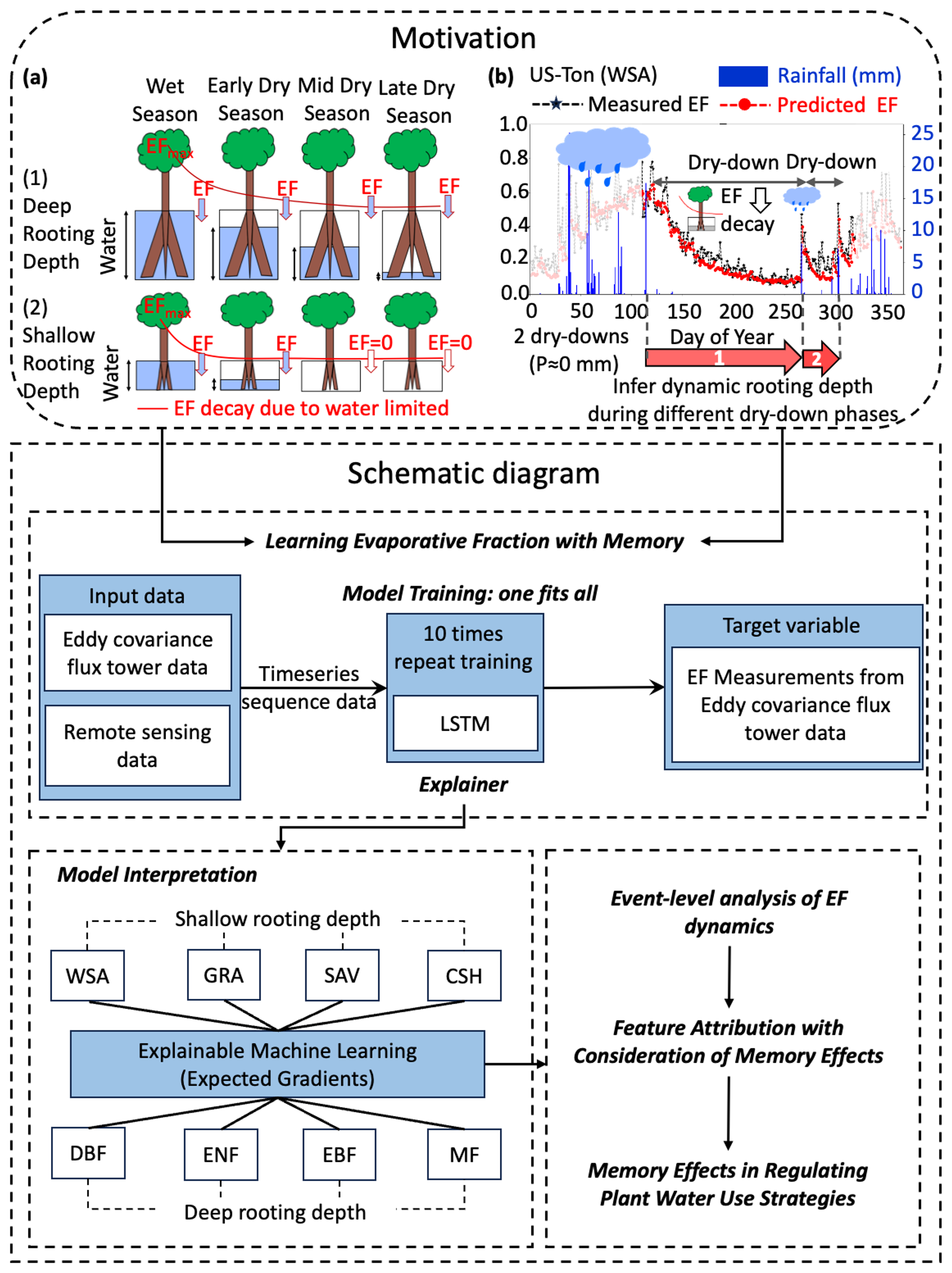
Figure 1 The motivation and schematic diagram of this study. Upper Panel: The motivation plot of this study. (a) indicates a water bucket model showing the EF decay during the dry downs. In the wet season, the precipitation fills up the vegetation water bucket and EF peaks. Then during the dry season, the vegetation will consume the available water storage during the wet season and thus EF decay could be observed. If the vegetation has a deep rooting depth, the EF decay will tend to be slow during the dry season. If the vegetation has a shallow rooting depth, the EF decay will tend to be fast during the dry season due to less available water storage compared to the deep rooting depth vegetation. Adapted from the Fig. 3 in Ichii et al. (2009). (b) indicates a field experiment on a woody savanna site (US-Ton). The observations support our hypothesis in plot (a). Precipitation provides the available water storage and EF peaks, then there's a EF decay during the dry downs. The rooting depth information is hidden in the slow and fast EF dry downs. If we could predict EF accurately, we could potentially infer information related to effective rooting-zone water storage and use EF as a direct water stress index. Lower Panel: The schematic diagram of this study. A long short-term model (LSTM) with memory effect is used here to capture the schemes expressed in the upper panel. The model is trained using eddy covariance flux tower data and remote sensing data. We train a general model for all the sites and then use explainable machine learning technique to analyze the drivers for each plant functional types and sites. Further investigations have been conducted to explore the relationship between memory effects and rooting depth, soil water holding capacity and aridity index across various PFTs.

2 Data Collection and Preprocessing

2.1 Eddy covariance measurements

We used 215 eddy-covariance sites from the combined ICOS (https://doi.org/10.18160/2G60-ZHAK, Warm Winter 2020 Team and ICOS Ecosystem Thematic Centre, 2022), AmeriFlux (https://ameriflux.lbl.gov/data/download-data/, last access: 22 August 2026), FLUXNET 2015 tier 1 dataset (https://fluxnet.org/data/fluxnet2015-dataset/, last access: 22 August 2026), covering 11 Plant Functional Types (PFTs) according to the IGBP (International Geosphere-Biosphere Programme) vegetation classification scheme (Loveland et al., 2000), including evergreen needleleaf forests (ENF), evergreen broadleaf forests (EBF), deciduous broadleaf forests (DBF), deciduous needleleaf forests (DNF), croplands (CRO), grasslands (GRA), savannas (SAV), woody savannas (WSA), closed shrublands (CSH), and mixed forests (MF), open shrub (OSH). The map of the site distributions is shown in Fig. S1 in the Supplement. Data for all the sites can be accessed via the links provided in Table S1 in the Supplement. We first exclude the sites without latent heat flux, sensible heat flux, surface shortwave incoming radiation, precipitation, vapor pressure deficit (VPD), air temperature, wind speed measurements from the analysis; then we drop all cropland and wetland sites, as cropland sites are usually affected by management practices such as irrigation, and wetland sites usually have a perched water table. Next, we only kept the sites which has more than 5 years of observations after we applied the data preprocessing steps (further aggregated from half-hourly to daily scale), detailed in the following paragraph. These preprocessing steps help to reduce the data imbalance issue in parameter optimizations during the training of the models. The final dataset consists of 90 sites: ENF (24), DBF (19), GRA (18), MF (8), SAV (7), OSH (6), WSA (4), and EBF (4). Each IGBP PFT label represents the dominant vegetation class within a tower footprint and therefore provides only a coarse site-level description of potentially mixed-species ecosystems.

2.2 Data Preprocessing Procedures of the Eddy-Covariance Dataset

The original sampling frequency of the data is half hourly. The data filter procedure can be summarized as follows: First, to reduce the noise in nighttime measurements, the original data is filtered with sensible heat flux >5 W m⁻² and shortwave incoming radiation >50 W m⁻² to select the daytime data only. Then, the original data is averaged to daily scale value (note that precipitation is calculated as the daily sum in 24 h). Secondly, we only keep days with a fraction of good quality data >0.8. The gaps in the time series for input features were interpolated using established methods (Reichstein et al., 2005; Vuichard and Papale, 2015). We also visually checked site by site to ensure that the signal-to-noise ratio is acceptable. For latent and sensible heat fluxes, we used the energy-balance-closure–corrected variables (LE_CORR and H_CORR) provided in the dataset, which adjust the fluxes to satisfy Rn $-G\approx LE+H$ following Wilson et al. (2002). We did not apply any additional masking based on an energy imbalance threshold. Due to the data limitation, only the shallowest soil moisture measurements were used for comparison with the evaporative fraction prediction dynamics during the drydown periods.

2.3 Evaporative Fraction Calculations

The Evaporative Fraction was calculated using the formula EF = $LE/$(H+LE), where LE represents the corrected latent heat flux and H the corrected sensible heat flux (Sect. 2.2). We assume the errors in LE and H exhibit comparable magnitudes, as suggested by previous studies (Foken, 2008; Hollinger and Richardson, 2005; Richardson et al., 2006), and are uncorrelated. This assumption enables to mathematically eliminate the errors associated with the lack of energy balance closure (Schwalm et al., 2010).

2.4 Auxiliary Datasets

The leaf area index (LAI) data were obtained from the MODIS MCD15A3H product using the Global Subset Tool (https://modis.ornl.gov/globalsubset/, last access: 22 August 2026), with a temporal resolution of 4 d. As LAI does not vary substantially within this period, the 4-d LAI values were used as daily inputs for our analyses.

Soil attribute data were derived from SoilGrids at a spatial resolution of 250 m, including clay, silt, and sand fractions (Poggio et al., 2021). Rooting depth information was obtained from the global dataset compiled by Tumber-Dávila et al. (2022). These rooting-depth observations are reported at the species level and are not spatially matched to the ecosystem-scale flux estimates within individual tower footprints.

Long-term evapotranspiration (ET) data used for dryness and wetness classification were extracted from the TerraClimate dataset via Google Earth Engine (Abatzoglou et al., 2018).

To characterize hydroclimatic conditions, we used both an aridity index (AI) and a seasonality index (SI). The aridity index was calculated as the ratio of mean annual precipitation to potential evapotranspiration (PET), with both variables derived from TerraClimate. Lower AI values indicate drier conditions, whereas higher values correspond to more humid environments.

The seasonality index (SI) was used to quantify the intra-annual variability of monthly precipitation. Specifically, SI was calculated as the ratio of the standard deviation to the mean of monthly precipitation within each year. Higher SI values indicate stronger seasonal variability (Teegavarapu, 2019).

These indices were used to characterize hydroclimatic gradients and seasonal variability in subsequent analyses.

3 Methodology

3.1 Long Short-Term Memory Model

A machine learning model using the Long Short-Term Memory architecture, which explicitly accounts for memory effects, is used to predict the daily scale EF. We test different combinations of hyperparameters, including the number of LSTM layers and neurons per layer, to determine the most appropriate model structure (Figs. S2, S3). The finalized model structure consists of 2 layers as follows: one LSTM layer with 128 neurons and one output dense layer with 1 neuron.

We choose dynamic variables including daily sum precipitation (P), daily mean wind speed (WS), daily mean surface shortwave incoming radiation (RAD), daily mean air temperature (T_a), daily mean VPD, LAI and site-specific static variables including soil properties and PFTs as the input features. In addition, annual mean P, annual mean RAD, annual mean T_a are also input of the model to account for climatic differences. The LSTM follows the standard formulation of Hochreiter and Schmidhuber (1997) as implemented in PyTorch, in which sigmoid activations are applied to the input, forget, and output gates, and tanh activations are applied to the cell-state and hidden-state transformations; the final output is produced by a single linear layer without additional non-linearity, which is standard practice for regression targets. The model was trained using the Adam optimizer (Kingma and Ba, 2015) with an initial learning rate of $\mathrm{1}\times {\mathrm{10}}^{-\mathrm{3}}$, decayed to $\mathrm{5}\times {\mathrm{10}}^{-\mathrm{4}}$ after epoch 10, a batch size of 64, and a mean squared error (MSE) loss function, for 50 training epochs.

3.2 Baseline model

To benchmark the predictive capacity of LSTM model, we choose three baseline approaches for comparisons: (1) a fully connected neural network (FNN) as a baseline for EF prediction. Like the process of defining the LSTM model structure, we tested different combinations of hyperparameters, including the number of fully connected layers and neurons per layer, while ensuring a fair comparison with the LSTM model. The final fully connected neural network model structure is as follows: it consists of two fully connected dense layers with 128 neurons and one output dense layer with 1 neuron (Figs. S2, S3). The length of time series sequence data is same with the input for the LSTM model. However, unlike the LSTM, the FNN treats the time-series inputs as fixed input features and does not contain recurrent or gating mechanisms to explicitly model temporal dependencies. It therefore serves as a baseline to test whether the improved performance of the LSTM arises from its ability to capture memory effects rather than simply from using the same input variables and sequence length. The FNN uses ReLU activations after each of the two hidden layers, with no activation applied to the output layer. It is trained with the same optimizer (Adam), learning rate schedule ($\mathrm{1}\times {\mathrm{10}}^{-\mathrm{3}}$ decayed to $\mathrm{5}\times {\mathrm{10}}^{-\mathrm{4}}$ after epoch 10), batch size (64), loss function (MSE), and number of epochs (50) as the LSTM model. (2) an EF climatology model. We calculate the climatology of EF as the baseline to show the LSTM's capacity in capturing the EF dynamics after the rain-pulse events. (3) a Standardized Precipitation Index (SPI)-based fitting model.

$$\begin{array}{}\text{(1)}& \mathrm{EF}={\mathit{\beta }}_{\mathrm{0}}\times \tan ({\mathit{\beta }}_{\mathrm{1}}\times \mathrm{SPI}+{\mathit{\beta }}_{\mathrm{2}})\end{array}$$

where β₀, β₁, and β₂ are three regression model parameters. The SPI-based model was included as a simple drought-index benchmark. Although SPI reflects antecedent precipitation anomalies, it cannot adequately capture the timing and magnitude of individual rain pulses or the subsequent post-rainfall EF dynamics, nor can it represent the joint effects of multiple meteorological drivers.

3.3 Training/Validation/Test Set Setups

We explored multiple training and validation strategies as benchmarking analyses rather than treating these strategies as interchangeable approaches. The datasets were partitioned using four complementary strategies: time-based split, time-based cross-validation (time-split CV), site-based cross-validation (site-split CV), and leave-one-site-out (LOSO). The time-based split and time-split CV evaluate temporal generalization within observed sites, whereas site-split CV and LOSO evaluate spatial transfer to unseen sites. The strategies are described as follows:

(1) Time-based split: The last year from each site was used for testing and the second-to-last year for validation, while the remaining site-years were used for training. (2) Time-based cross-validation: Each site's time series was divided into five contiguous segments. The model was trained on four segments and tested on the remaining segment, iteratively across all folds. (3) Site-based cross-validation: Sites were randomly divided into five folds, and models were trained on four folds and tested on the remaining fold. This strategy evaluates spatial generalization across different ecosystems. (4) Leave-one-site-out: The model was iteratively trained on all sites except one and tested on the excluded site. All dynamic and static input variables were z-score standardized using the mean and standard deviation computed from the training set, with the same statistics then applied to the validation and test sets to avoid information leakage.

To quantify the role of memory and improve model robustness, we trained ensembles of LSTM models with varying sequence lengths. The memory length was varied from 10 to 360 d at 30-d intervals, with an additional experiment at 365 d (Fig. S3), to systematically evaluate the influence of temporal context on EF prediction. For each candidate memory length, we trained 10 models that differed only in the random initialization of weights and biases. This ensemble approach reduces stochastic variability associated with neural network training and provides an estimate of prediction uncertainty. The improved performance of the ensemble mean highlights its ability to capture complex nonlinear interactions and memory effects from high-dimensional input features – patterns that are often challenging for traditional process-based models to reproduce. The use of ensemble learning is a well-established strategy for improving generalization and mitigating overfitting in complex nonlinear systems (Dietterich, 2000), and has been widely adopted in Earth system modeling studies (e.g., Kraft et al., 2019; Jung et al., 2019; Jiang et al., 2022a; Nelson et al., 2024). We therefore recommend using an ensemble approach for both final prediction and model interpretation.

Early stopping was applied during training to avoid overfitting and select the optimal model. The final EF prediction for each configuration was obtained as the ensemble mean across the 10 models. After comparing predictive performance across all memory lengths, the 365-d configuration yielded the highest skill. Therefore, all subsequent analyses are based on the 10-member ensemble trained with this optimal sequence length.

3.4 Soil moisture drydown identification

We define soil-moisture dry-down events as rainfall-free periods during which soil moisture first shows an immediate post-rain pulse increase and then decreases continuously for at least seven consecutive days until the next rainfall event. At each flux tower site, we retained drydown events for analysis if soil moisture decreased continuously for at least 7 d after rainfall, following the criteria used in previous studies (Fu et al., 2024; McColl et al., 2017). We also tested more stringent thresholds of 9 and 11 d for the minimum drydown duration, and found that the results remained consistent.

3.5 Expected Gradients (EG)

We employed the explainable machine learning method Expected Gradients (EG) (Erion et al., 2021) to interpret the black-box model and quantify feature importance at each time step. This approach reveals the specific contributions of inputs to daily EF predictions. Compared to permutation feature importance, EG allows the temporal model to decompose overall feature importance into specific contributions at each time step (Jiang et al., 2022b; Molnar, 2019). This detailed analysis enables us to examine plant responses across varying memory effects under extreme events or environmental conditions, a capability that is not available in non-temporal models.

EG extends Integrated Gradients (IG) by addressing its sensitivity to baseline selection. Instead of relying on a single fixed baseline, EG samples baseline inputs from a reference data distribution (e.g., the training dataset). The attribution score for the i-th feature is then obtained by integrating the gradients across all possible baseline inputs, weighted by the distribution density (Erion et al., 2021; Jiang et al., 2022a; Sundararajan et al., 2017).

The EG method could unbox the LSTM-based machine learning model and trace back the specific contributions of the inputs and assign an importance score to each feature at each time prior to the predictions. A positive EG score could indicate that the feature substantially increases the Evaporative Fraction predictions (e.g., that precipitation at the most proximate time may contribute more to current Evaporative Fraction projections than precipitation at an earlier time). A negative EG score indicates that the feature decreases the EF predictions. An EG score close to zero indicates little influence on the EF predictions. This way, this framework not only quantifies overall feature importance but also resolves its temporal structure, revealing how the influence of predictors evolves over time. More specifically, it implies that temporal length of the input features will be considered for the EF predictions for different kinds of PFTs, in which hint the response of plant with different rooting depths during specific extreme events or environmental conditions, e.g., droughts with different severity level.

The IG score for the input feature x (e.g., the specific contribution of precipitation at the ith time step) is formulated as:

$$\begin{array}{}\text{(2)}& {\varnothing }_i\left(x\right)=\left(x_i-x_i^{\prime }\right)\times {\int }_{\mathit{\alpha }=\mathrm{0}}^{\mathrm{1}}{\displaystyle \frac{\partial F(x^{\prime }+\mathit{\alpha }\times \left(x-x^{\prime }\right))}{\partial x_i}}\mathrm{d}\mathit{\alpha }\end{array}$$

Where $\frac{\partial F(x^{\prime }+\mathit{\alpha }\times \left(x-x^{\prime }\right))}{\partial x_i}$ denotes the local gradient of the network F at a point interpolated from a baseline input ($x^{\prime }\text{when}\mathit{\alpha }=\mathrm{0}$), which is meant to represent the “absence” of the feature input, to the target input (x, when α=1). Note that the IG value is completeness and add up to the difference between the output of F at the target input x and the baseline input x^′, i.e., $\sum _i{\varnothing }_i\left(x\right)=F\left(x\right)-F\left(x^{\prime }\right)$. Therefore, the model output can be decomposed into the sum of features' individual contributions, and it enables us to examine the contribution of a group of features by summing up their individual IG scores.

Due to the integral, the original definition of IG is incalculable. Therefore, the implementation of the method in practice uses approximated value by replacing the integral with the summation:

$$\begin{array}{}\text{(3)}& \begin{array}{rl}{\varnothing }_i^{\mathrm{approx}}& \left(x\right)=\left(x_i-x_i^{\prime }\right)\times \\ & {\sum }_{k=\mathrm{1}}^m{\displaystyle \frac{\partial F\left(x^{\prime }+\frac{k}{m}\times \left(x-x^{\prime }\right)\right)}{\partial x_i}}\times {\displaystyle \frac{\mathrm{1}}{m}}\end{array}\end{array}$$

where m defines a number of interpolation steps.

Formally, given a baseline distribution D, the EG of the i-th feature can be calculated by integrating the gradients with all possible baseline inputs $x^{\prime }\in D$ weighted by the density function p_D, which is expressed as:

$$\begin{array}{}\text{(4)}& {\mathit{\varphi }}_i^{\mathrm{EG}}(f,x)={\int }_{x^{\prime }}\left({\mathit{\varphi }}_i^{\mathrm{IG}}(f,x,x^{\prime })\times p_{\mathrm{D}}\left(x^{\prime }\right)\mathrm{d}{x}^{\prime }\right)\end{array}$$

The formulation is therefore called Expected Gradients, and can be reformulated as

$$\begin{array}{}\text{(5)}& \begin{array}{rl}{\mathit{\varphi }}_i^{\mathrm{EG}}(f,x)& =E_{{{\mathrm{x}}^{\prime }}_{\sim }D,\mathit{\alpha }\sim U(\mathrm{0},\mathrm{1})}\left[(x_i-{x^{\prime }}_i)\right.\\ & \left.\times {\displaystyle \frac{\partial f(x^{\prime }+\mathit{\alpha }(x-x^{\prime }\left)\right)}{\partial {x^{\prime }}_i}}\right]\end{array}\end{array}$$

where U(0,1) denotes the uniform distribution between 0 and 1.

In this study, we use the library captum (https://github.com/pytorch/captum, last access: 22 August 2026) to obtain the EG scores for each feature at each time step.

3.6 Memory effect quantification

To summarize the Expected Gradients (EG) into interpretable metrics of driver importance and memory effects, we aggregated the EG scores across both variables and antecedent time steps. Because EG values can be positive or negative depending on whether a given predictor at a given lag increases or decreases the EF prediction, we used the absolute values of EGs when quantifying contribution magnitude. This allows us to focus on the strength of the contribution rather than its sign and prevents positive and negative attributions from canceling each other out.

First, to quantify the overall relative importance of each predictor (Figs. 6 and 7), we summed the absolute EG scores over all antecedent time steps for each variable. For a given variable i, its relative contribution was calculated as

$$\begin{array}{}\text{(6)}& {\mathrm{RC}}_i={\displaystyle \frac{{\sum }_{t=\mathrm{0}}^{\mathrm{365}}\left|{\mathrm{EG}}_i\left(t\right)\right|}{{\sum }_{j\in V}\sum _{t=\mathrm{0}}^{\mathrm{365}}\left|{\mathrm{EG}}_j\left(t\right)\right|}}\times \mathrm{100}\mathit{\%}\end{array}$$

where V denotes the full predictor set, including precipitation (P), air temperature (Ta), shortwave radiation (RAD), vapor pressure deficit (VPD), wind speed (WS), and LAI. This normalization yields the percentage contribution of each variable to the EF prediction. For Fig. 6, these normalized contributions were first calculated for each site-year in the test set and then summarized by plant functional type (PFT). For Fig. 7, the same EG-based contributions were summarized site by site to show site-level variability in driver importance.

To further isolate antecedent or memory contributions, we defined a cumulative memory contribution metric as the fraction of total absolute EG attribution arising from lags deeper than a given antecedent threshold k. Specifically, for a set of variables S, we computed

$$\begin{array}{}\text{(7)}& \mathrm{PC}\left(S,k\right)={\displaystyle \frac{{\sum }_{i\in S}{\sum }_{t=k}^{\mathrm{365}}\left|{\mathrm{EG}}_i\left(t\right)\right|}{{\sum }_{i\in S}{\sum }_{t=\mathrm{0}}^{\mathrm{365}}\left|{\mathrm{EG}}_i\left(t\right)\right|}}\times \mathrm{100}\mathit{\%}\end{array}$$

where EG_i(t) is the Expected Gradient attribution of variable i at lag t, and k defines the lower bound of the antecedent window. Thus, PC(S,k) measures the percentage of total contribution attributable to lags deeper than k days. In this study, k was varied systematically to characterize how attribution magnitude decays with lag, thereby yielding a memory decay curve for each site or PFT. A larger value of PC(S,k) at large k indicates a stronger long-term memory effect.

This framework can be applied to different variable sets depending on the analysis objective. For aggregated memory analyses across all dynamic predictors, we used S= {P, Ta, RAD, VPD, WS, LAI}. This enables us to aggregate EGs and quantify antecedent memory contributions either for an individual driver or for the full predictor set. Figures 8–10 use the full dynamic predictor set.

For Fig. 8, we used the decay of PC(S,k) with increasing k for the full dynamic predictor set, S= {P, Ta, RAD, VPD, WS, LAI}, to construct memory decay curves. To facilitate comparison across sites and PFTs, we defined characteristic decay timescales t₅₀ and t₂₀ as the antecedent days required for the normalized memory contribution to decay to 50 % and 20 % of its initial value of 100 %, respectively. These decay metrics were calculated at the site level and summarized by PFT for panels a–c. For panels d–i, observed maximum rooting depth and EG-derived decay timescales were independently aggregated within common biome categories at the 20th, 50th, and 80th percentiles, following Stocker et al. (2023) and Olson et al. (2001). This distribution-based comparison reduces the influence of the heavy-tailed rooting-depth distribution and avoids direct point-to-point matching between species-level rooting-depth observations and ecosystem-scale flux-site memory estimates, which are not spatially matched.

In addition to the memory decay timescales, for Figs. 9 and 10 we quantified the memory effect using the cumulative antecedent contribution from lags 7 to 365 d relative to the total contribution from lags 0 to 365 d. In these analyses, we used the full dynamic predictor set, S= {P, Ta, RAD, VPD, WS, LAI}. This memory effect contribution metric was then related to rooting depth, soil sand fraction, seasonality index, and aridity index to assess whether ecosystems with deeper rooting systems, greater soil water-holding capacity, or wetter and less seasonal climates exhibit stronger antecedent memory effects.

Overall, this EG-based summarization framework enables us to move from raw time-resolved attribution scores to interpretable ecological metrics, including variable importance, antecedent contribution fractions, and memory decay timescales, thereby providing the methodological basis for Figs. 6–10.

4 Results

4.1 Model Performance Across All Plant Functional Types of LSTM with benchmark models

Figure 2 shows the performance of the LSTM model with a memory length of 365 d under different training and validation strategies. Overall, the model achieved good NSE values for most sites across all strategies. For all periods, the time-based split yielded the highest median site-level NSE (0.63), followed by time-based cross-validation (0.53), LOSO (0.51), and site-based cross-validation (0.44). Under the time-based split, the FNN reached a median NSE of 0.53, whereas the climatology and SPI-based models yielded median NSE values of −0.08 and −0.11, respectively. During drydown periods, model performance was slightly lower than for all periods, but remained above 0.45 for all LSTM evaluation strategies. The median NSE was highest for the time-based split (0.55), followed by LOSO (0.53), time-based cross-validation (0.52), and site-based cross-validation (0.45). Under the same setting (time-based split), the FNN achieved a median NSE of 0.47, whereas the climatology and SPI-based models showed lower performance, with median NSE values of −0.08 and −0.21, respectively. For non-drydown periods, the ranking of strategies was similar. The time-based split again gave the highest median NSE (0.61), followed by time-based cross-validation (0.51), LOSO (0.48), and site-based cross-validation (0.42). The FNN yielded a median NSE of 0.55, while the climatology and SPI-based models showed median NSE values of −0.14 and −0.13, respectively. Across all three conditions, the LSTM under the time-based split consistently showed the strongest performance, while site-based cross-validation yielded the lowest median NSE among the four LSTM evaluation strategies. In all cases, the LSTM also outperformed the benchmark models, particularly the climatology and SPI-based approaches.

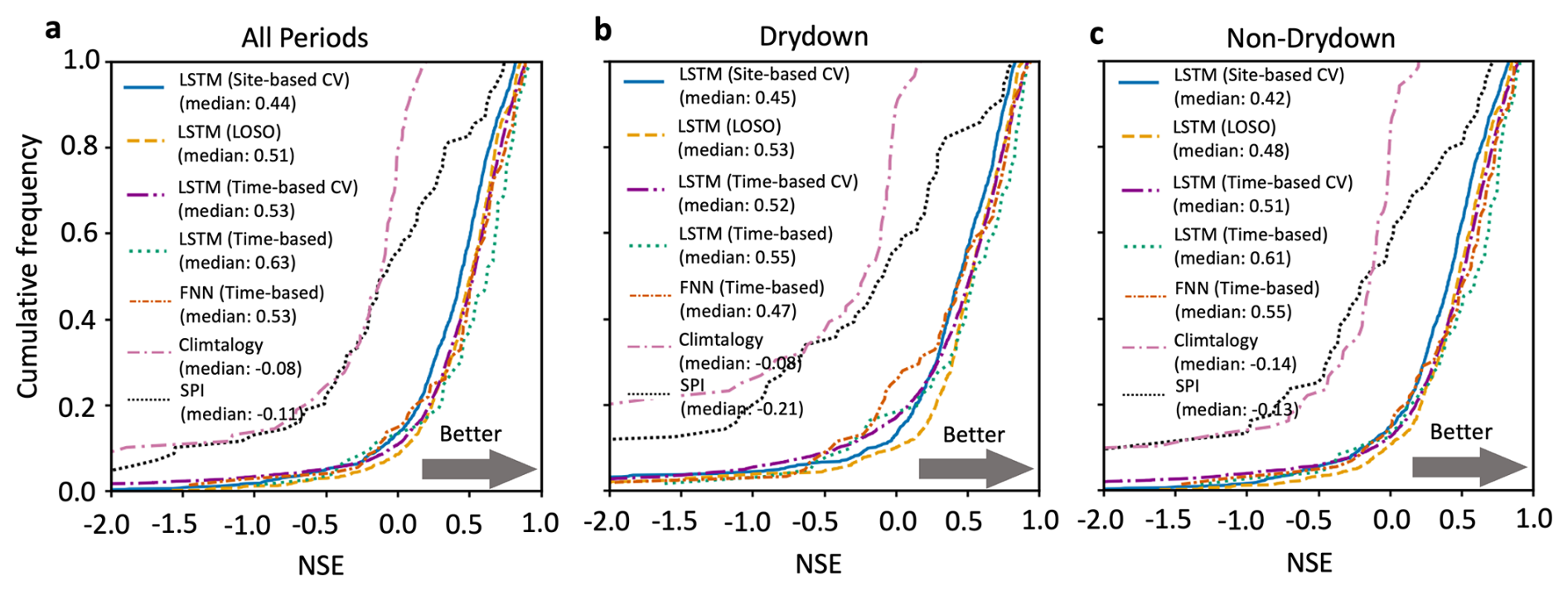
Figure 2 LSTM model performance evaluated on the test set under different training strategies. Cumulative distribution functions (CDFs) of site-level Nash–Sutcliffe efficiency (NSE) across sites for (a) all periods, (b) drydown periods, and (c) non-drydown periods. Four strategies are compared: site-based CV, LOSO, time-based CV, and time-based split. The benchmark models, including FNN, climatology, and SPI-based fitting, are also included under the time-based split setting for comparison. NSE is computed separately at each site, and the resulting distributions characterize the variability in model performance across sites. Median NSE values are indicated in the legends. Higher NSE values indicate better performance.

We further evaluated model performance across broad vegetation groups and hydrological conditions to assess whether the LSTM consistently outperformed the benchmark models. Figure 3 shows the mean site-level NSE for grassland, shrub/savanna, and forest groups across all periods, drydown periods, and non-drydown periods. In all vegetation groups and under all conditions, the LSTM yielded the highest NSE among the four models.

In grassland sites, the LSTM achieved mean NSE values of 0.42, 0.67, and 0.28 for all periods, drydown periods, and non-drydown periods, respectively, compared with 0.32, 0.58, and 0.23 for the FNN. The SPI-based and climatology-based models performed substantially worse, with negative NSE values in all three cases. In shrub/savanna sites, the LSTM showed the highest performance overall, with mean NSE values of 0.73, 0.71, and 0.74, whereas the FNN reached 0.61, 0.64, and 0.64, respectively. Again, the SPI-based and climatology-based models yielded negative NSE values across all conditions. In forest sites, the LSTM remained the best-performing model, with mean NSE values of 0.48, 0.47, and 0.42, compared with 0.41, 0.36, and 0.37 for the FNN. The SPI-based model was near zero or negative, and the climatology-based model was consistently negative. These results show that the LSTM more accurately captures EF dynamics than the benchmark models across vegetation groups and hydrological conditions.

Overall, the LSTM consistently outperformed the benchmark models across training strategies, vegetation groups, and hydrological conditions. Because our primary objective was to investigate EF dynamics and memory effects, we used the time-based split for the subsequent analyses, as it provided both strong predictive skill and a more suitable basis for an interpretable explainer model at each site. We acknowledge, however, that for spatial upscaling and transfer to unseen sites, site-level training strategies should be further considered in future work.

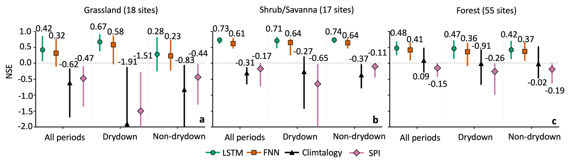
Figure 3 Comparison of model performance between the LSTM and baseline models. Panels a–c show results for grassland (GRA), shrub/savanna (WSA, OSH, and SAV), and forest (DBF, EBF, ENF, and MF) groups, respectively. Within each panel, model performance is summarized for all periods, drydown periods, and non-drydown periods. Symbols denote the mean site-level Nash–Sutcliffe efficiency (NSE) of each model, calculated by first computing NSE separately at each site and then averaging across all sites within each vegetation group. Error bars represent the interquartile range (25th to 75th percentiles) across sites. Green circles show the LSTM performance under the time-based split strategy, orange squares show FNN under the time-based split strategy, black triangles show the climatology-based model, and pink diamonds show the SPI-based model. Higher NSE values indicate better agreement between predicted and observed evaporative fraction (EF). Site counts are shown in parentheses.

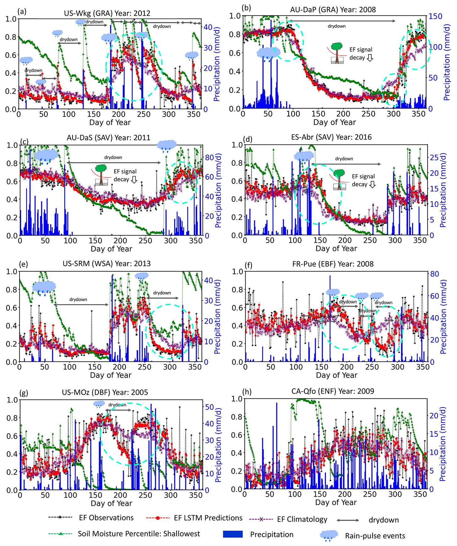
Figure 4 Prediction of Evaporative Fraction Dynamics Across Various Plant Functional Types. Daily time series of Evaporative Fraction (EF) dynamics for several cases of dry-down periods, as estimated by machine learning models considering memory effects. Blue bars show the observed daily sum precipitation (P), black curves show EF observations, red curves show EF predictions, green curves show soil moisture percentiles of the shallowest soil depth. The x-axis represents the day of year (DOY) of the whole year. Labels in the panels show the auxiliary information of the detected dry-down periods (GRA: grassland, WSA: woody savanna, SAV: savanna, DBF: deciduous broadleaf forest, ENF: evergreen needleleaf forest). The daily volumetric water content values are converted into percentiles, indicating the fraction of daily values lower than a specific value. Thus, the 100th percentile (or a percentile value of 1) represents the wettest soil conditions observed at a specific site throughout the study period, and the 0 percentile signifies the driest soil conditions. The length of time sequence input is set as 365 d for the machine learning model. The EF predictions here are using the ensemble mean EF predictions of 10 models with different initializations. Shaded areas represent regions of predictions uncertainty in the 25 %–75 % quartiles of these 10 repeat training models. Note all the results shown here are from the test set.

Our model adeptly captures the observed EF dynamics as observed in the unseen site-years, particularly during soil moisture dry-down periods across grassland, savanna and woody savanna sites, as illustrated in Fig. 4. The decay in EF predictions aligns with the observed decline in shallow soil moisture (only shallow soil moisture observations are used here for comparisons due to the data limitation). Consequently, EF peaks, and then gradually decreases at varying rates during drydown intervals. For example, grasslands, with typically shallow roots, exhibit a faster EF decay compared to savannas (Fig. 4). However, we also note the diversity of climatic environments in which the different grassland sites are situated. For instance, AU-DaP experiences sufficient precipitation only in certain seasons, whereas precipitation at AT-Neu is more evenly distributed throughout the entire year (Fig. S5). Some grassland sites receive sufficient rainfall during the whole years like the deciduous broadleaf and evergreen broadleaf forest sites, which leads to differences in the characteristics of their EF drydowns. In contrast to the sporadic rainfall patterns typical of grasslands and savannas, deciduous broadleaf forest and evergreen broadleaf forest sites experience abundant precipitation throughout the year, and this consistent moisture supply contributes to substantial variability in observed EF.

The contribution of each individual time step indicated by the Expected Gradients (see Methods) clearly shows the impact of previous rainfall on the current EF predictions (Fig. 5a, b, c). Expected Gradients reveal the contributions of antecedent climate variables, including precipitation, air temperature, vapor pressure deficit (VPD), net radiation, and LAI, to current EF predictions. During a long drydown event at a grassland site (AU-DaP, 5 October 2013), precipitation around 5 April 2013 shows a positive contribution to EF, while VPD and LAI also exhibit notable contributions. Across different sites and vegetation types, similar patterns are observed. In an evergreen needleleaf forest site (CA-TP1, 11 April 2014), a low-temperature event around 11 January 2014 is associated with EF variations approximately three months later, indicating a temporal lag in the response. This reflects the positive impact of previous precipitation (lag effect), especially closest to the prediction time, and negative impact of dry spells to EF predictions (Fig. 5a). Additionally, past episodes of extremely low temperature may also suppress vegetation functioning, as reflected in EF predictions during April at the CA-TP1 site (Fig. 5d). We summarize all the explainable EGs for all the sites in the following figures (Sect. 4.2).

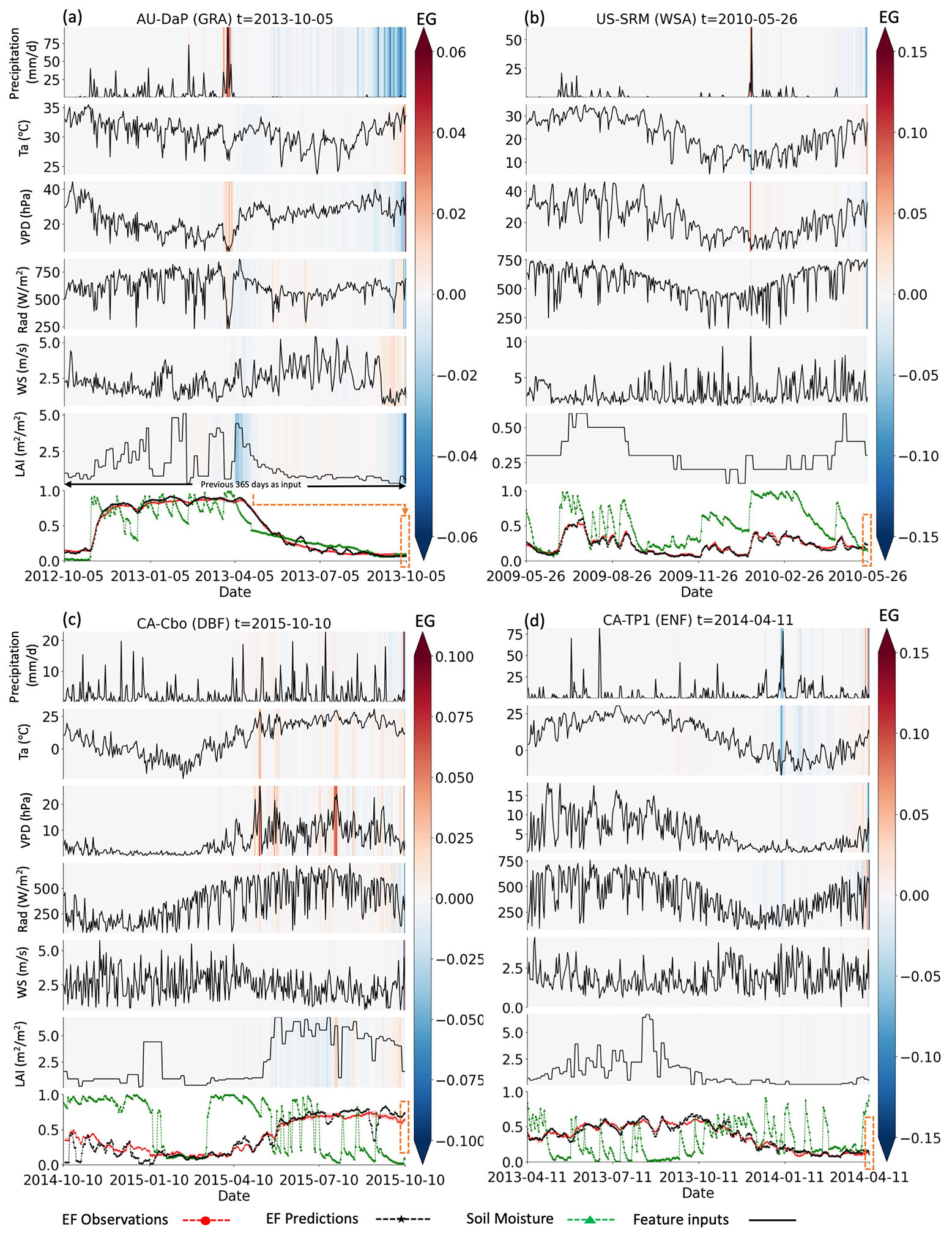
Figure 5 Examples of memory effects revealed by Expected Gradients. (a) A grassland site (AU-DaP, 5 October 2013). The LSTM model uses the previous 365 d of input data (from 5 October 2012 to 5 October 2013) to predict EF on 5 October 2013. Expected Gradients illustrate the contributions of antecedent climate variables, e.g., precipitation, air temperature, vapor pressure deficit (VPD), net radiation, and LAI, to the current EF prediction. During this long drydown event, precipitation around 5 April 2013 shows a positive contribution to EF. VPD and LAI also exhibit notable contributions. (b) A woody savanna site (US-SRM, 26 May 2010); (c) a deciduous broadleaf forest site (CA-Cbo, 10 October 2015); and (d) an evergreen needleleaf forest site (CA-TP1, 11 April 2014). Expected Gradient patterns across all sites are summarized in the subsequent figures.

4.2 Drivers of EF Dynamics Incorporating Memory Effects

Delving into the causes of rapid and gradual EF decreases, we analyze the trained EF model using explainable machine learning techniques, namely Expected Gradients (Erion et al., 2021; Molnar, 2019; Sundararajan et al., 2017). EG is a method for attributing the prediction of a neural network to its input features by integrating gradients along the path from randomly sampled baselines to the actual input and averaging over these attributions. This analysis not only revealed the controlling factors in predicting EF but also delineated the temporal influences, allowing us to ascertain the general feature importance alongside the distinct contributions to each individual time step. Consequently, the feature importance obtained through EGs inherently includes the memory contributions from historical periods for each variable, thus potentially considering the memory effect and the legacy effect. First, we summarize the EGs by calculating the relative contribution for each variable (in %). This is achieved by dividing the total sum of absolute EGs for each variable. For all the sites put together, the absolute EGs identified precipitation (25 %) and air temperature (22 %) as the most two influential drivers. This is followed by radiation (21 %), vapor pressure deficit (18 %), wind speed (7 %), and leaf area index (6 %). However, we also note that the significance of input features importance varies among different sites, different PFTs and climatic regions (Figs. 6, 7). In general, the water controls, i.e., precipitation, VPD are the two main drivers for most of woody savanna, savanna, open shrubland and grassland sites, whereas air temperature emerges as the dominant factor for most forest sites for deciduous broadleaf forest, evergreen needleleaf forest and mixed forest sites (Fig. 7). These driver patterns are broadly consistent with the distinction between more water-limited systems, such as savannas, shrublands, and many grassland sites, and less water-limited or more energy-limited forest systems, although substantial site-level variability remains within each PFT.

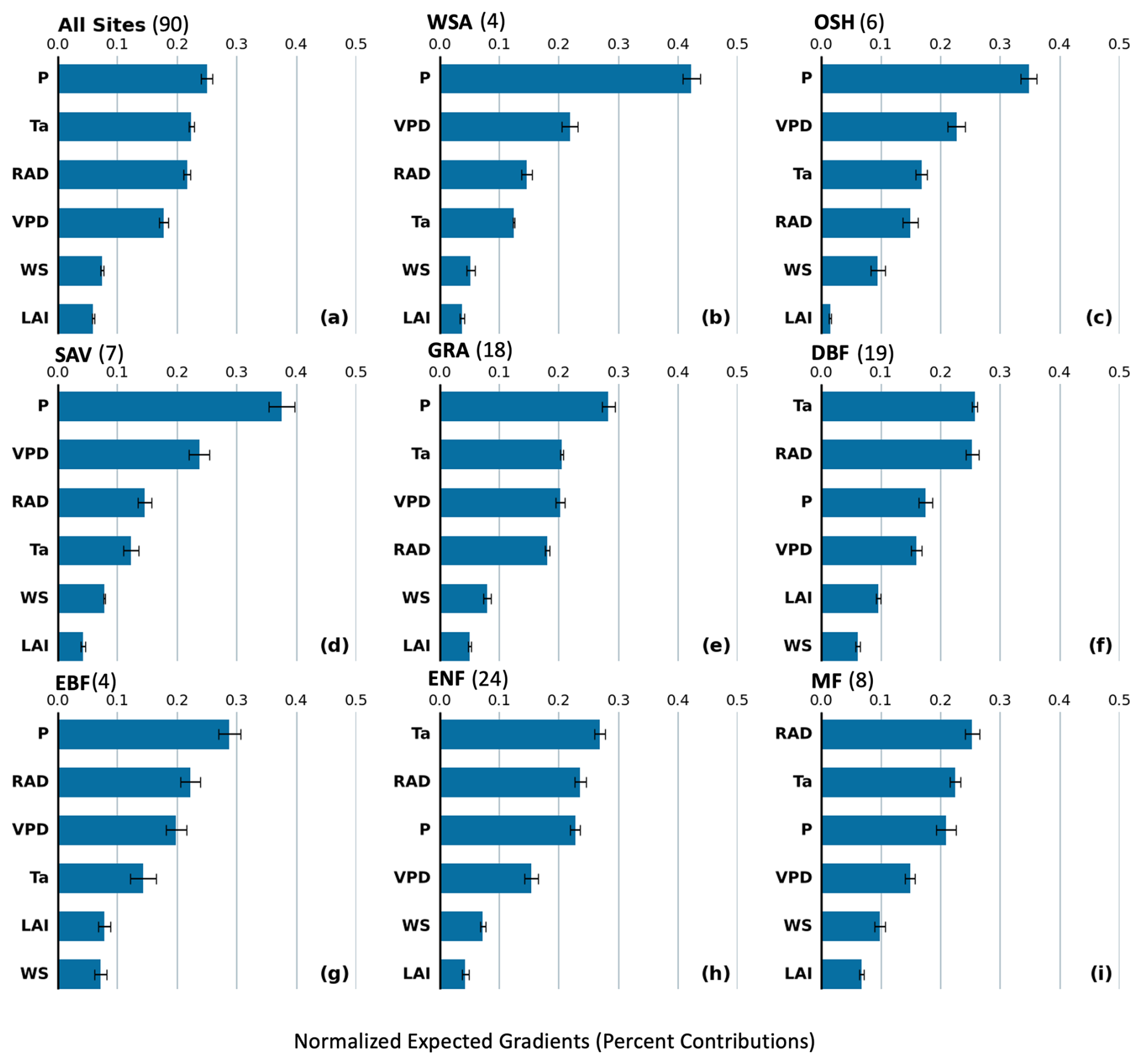
Figure 6 Feature Importance Revealed by the Temporal Evaporative Fractions Model Considering the Memory Effect. a indicates the overall feature importance across all the plant functional types. b, c, d, e, f, g, h, i represents the feature importance for woody savanna (WSA), open shrubland (OSH), savanna grassland (SAV), deciduous broadleaf forest (DBF), evergreen broadleaf forest (EBF), evergreen needleleaf forest (ENF), mixed forest (MF). Note that the EG values are normalized by percent contributions, that is, divided by the total sum of absolute EGs for all the variables shown here in each plot. Thus the values here indicate a relative percent contribution (e.g., 0.3 means 30 %). Site counts are shown in parentheses.

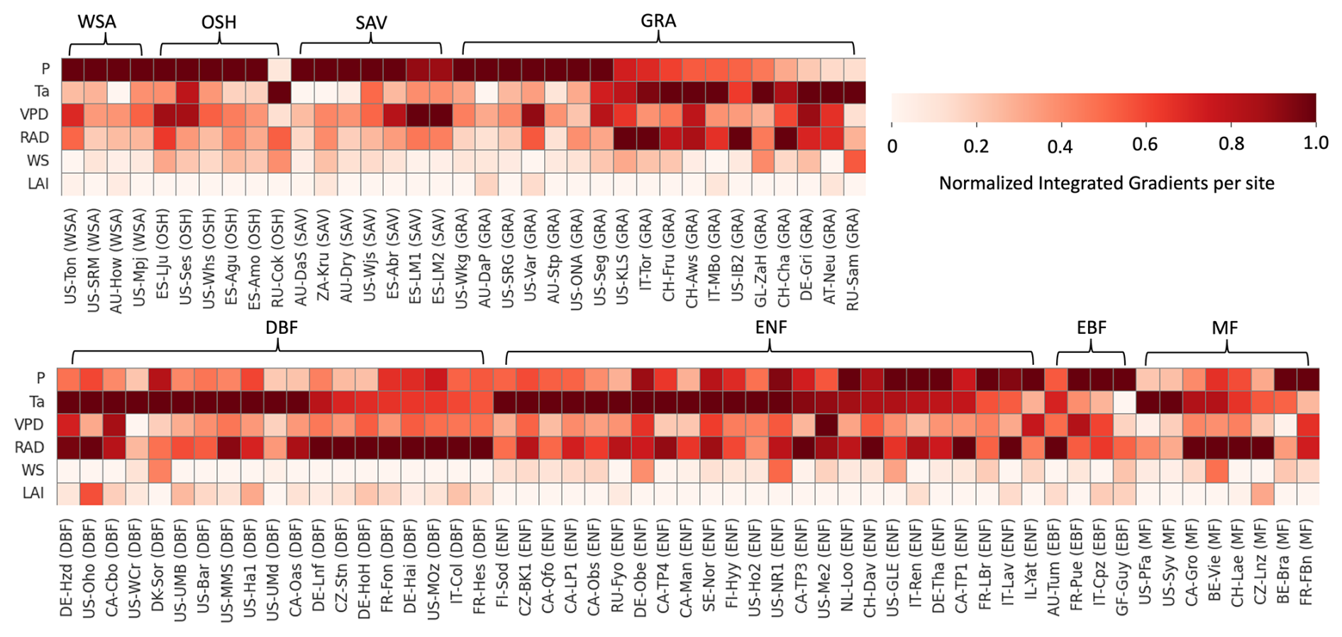
Figure 7 Feature Importance Revealed by the Temporal Evaporative Fractions Model Considering the Memory Effect for each site. Note that the absolute EG values are normalized by using minimum and maximum EG values in each site. Thus, the values here with 1 most important, while 0 least important to the evaporative fraction predictions.

4.3 Memory Effects: Uncovering Hidden Mechanisms in Plant Water Use Strategies

To further characterize memory effects across vegetation groups, we summarized the decay of normalized antecedent contributions and derived memory decay curves for each site (Methods). From these curves, we defined the characteristic decay timescales t₅₀ and t₂₀ as the number of antecedent days required for the normalized memory contribution to decay from its initial value of 100 % to 50 % and 20 %, respectively (Fig. 8). Clear differences in memory decay patterns were observed among grassland, shrub/savanna, and forest groups. In general, grassland sites showed the fastest decay of antecedent contributions, whereas shrub/savanna and forest sites exhibited slower decay, with substantial contributions persisting to longer lags. The representative insets illustrate these differences in decay timescales. In the grassland example, t₅₀ and t₂₀ were 8 and 34 d, respectively. In the shrub/savanna example, the corresponding values were 8 and 46 d. In the forest example, the decay was much slower, with t₅₀=41 d and t₂₀=216 d. At the group level, the mean decay curves also showed a progressive shift toward longer memory timescales from grassland to shrub/savanna and forest systems.

To compare the ecosystem-scale memory metrics with species-level observations of maximum rooting depth, both variables were independently aggregated within common biome categories at the 20th, 50th, and 80th percentiles, following Stocker et al. (2023) and Olson et al. (2001). Significant positive relationships were found between rooting depth and t₅₀ at the 20th (r=0.89, P=0.00725) and 80th percentiles (r=0.90, P=0.00607), and between rooting depth and t₂₀ at the 20th percentile (r=0.80, P=0.0321; Fig. 8d–i). Relationships at the remaining percentiles were weaker and not statistically significant. Substantial within-group variability nevertheless remained. These results therefore indicate positive biome-level associations at selected quantiles rather than direct site- or species-specific estimates because the datasets are not spatially matched.

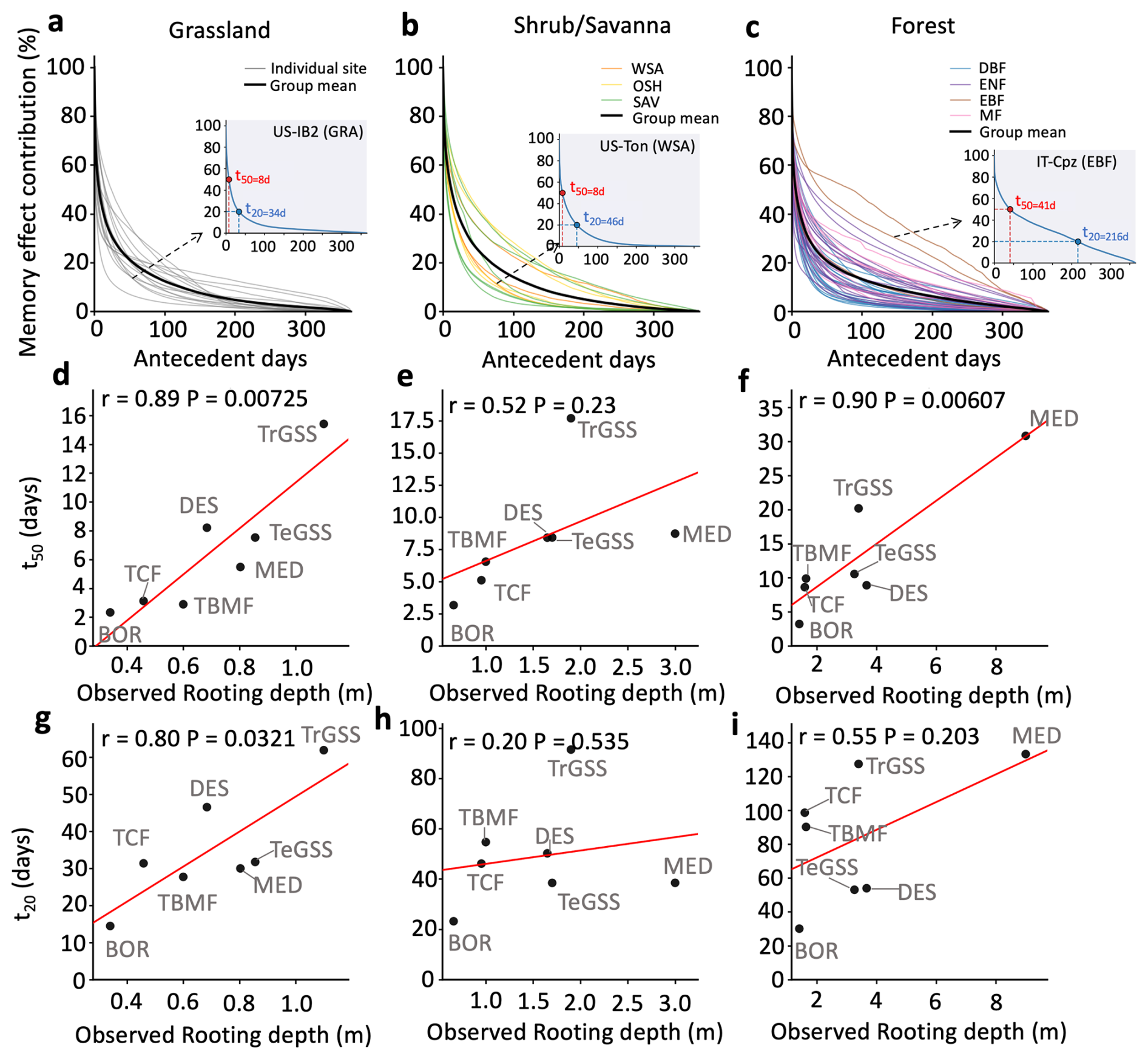
Figure 8 Memory effect decay of antecedent contributions across plant functional groups and its relationship with observed rooting depth. Panels (a)–(c) show the decay of normalized antecedent memory contributions, derived from the full dynamic predictor set S= {P, Ta, RAD, VPD, WS, LAI}, with increasing lag days for grassland, shrub/savanna, and forest groups, respectively. Thin colored or gray lines denote individual sites, and thick black lines denote the group mean. Insets illustrate representative examples, with t₅₀ and t₂₀ defined as the antecedent days required for the normalized contribution to decay to 50 % and 20 % of its initial value (100 %), respectively. Panels (d)–(f) show relationships between observed maximum rooting depth and t₅₀ aggregated at the 20th, 50th, and 80th percentiles, while panels (g)–(i) show the corresponding relationships for t₂₀. Each labeled point represents a biome-level aggregation. Biome abbreviations are BOR, boreal forests/taiga; TCF, temperate conifer forests; TBMF, temperate broadleaf and mixed forests; DES, deserts and xeric shrublands; TeGSS, temperate grasslands, savannas and shrublands; TrGSS, tropical and subtropical grasslands, savannas and shrublands; and MED, Mediterranean forests, woodlands and scrub. red lines indicate linear fits across biomes, with Pearson's r and corresponding P values shown in each panel. Following Stocker et al. (2023) and Olson et al. (2001), observed maximum rooting depth and memory decay timescales were independently aggregated within common biome categories at the 20th, 50th, and 80th percentiles to reduce the influence of the heavy-tailed rooting-depth distribution and avoid direct point-to-point comparison between species-level rooting-depth observations and ecosystem-scale flux-site memory estimates, which are not spatially matched.

In addition to the memory decay timescales, for Figs. 9 and 10 we quantified the memory effect using the cumulative antecedent contribution from lags 7 to 365 d relative to the total contribution from lags 0 to 365 d. In these analyses, we used the full dynamic predictor set, S= {P, Ta, RAD, VPD, WS, LAI}. This memory effect contribution metric was then related to rooting depth, soil sand fraction, seasonality index, and aridity index to assess whether ecosystems with deeper rooting systems, greater soil water-holding capacity, or wetter and less seasonal climates exhibit stronger antecedent memory effects. Memory effects varied substantially within most classes, while land-cover classifications only crudely capture the heterogeneous responses of vegetation to water stress (Konings and Gentine, 2017).

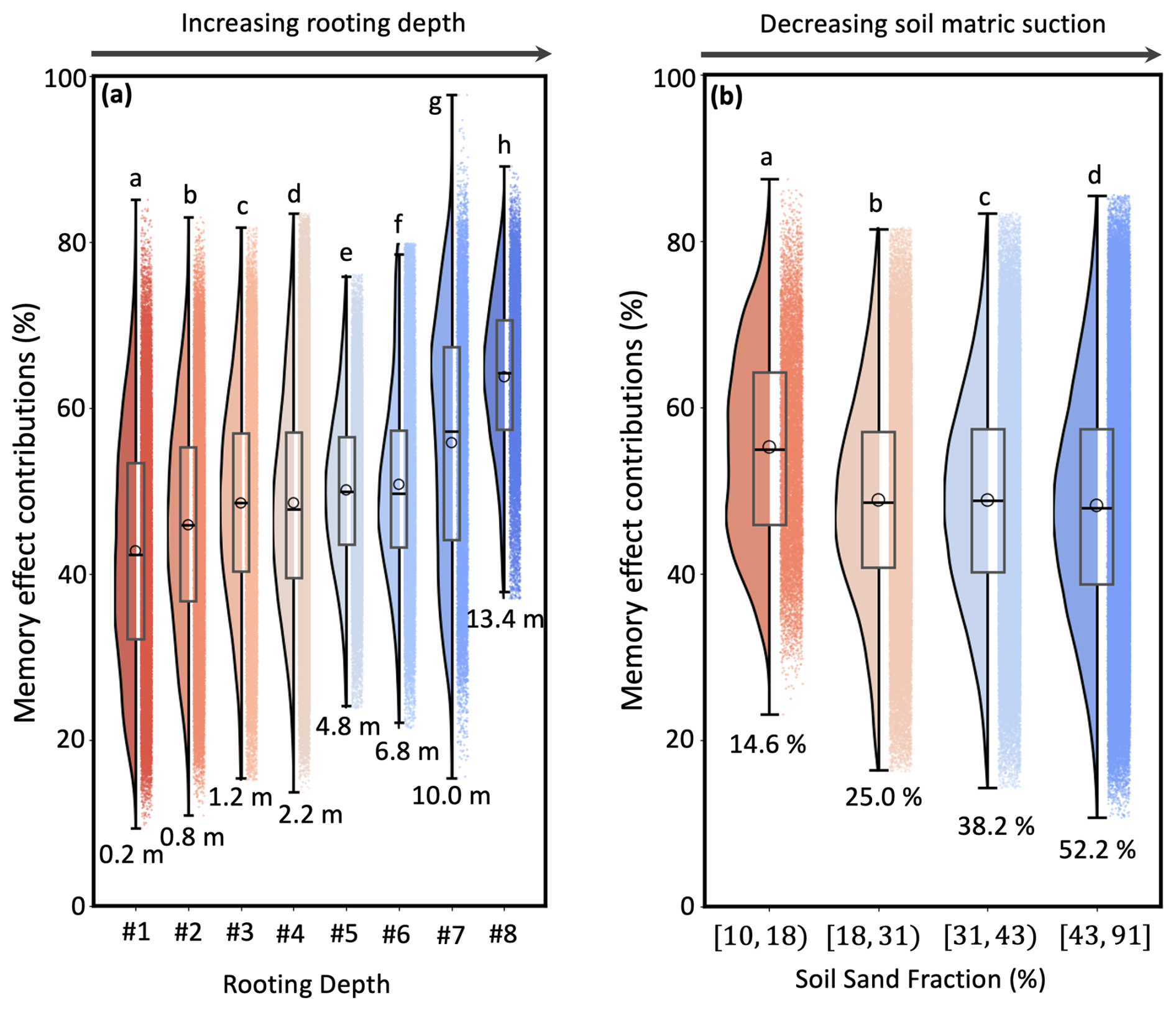
Figure 9 The Relationship Between Rooting Depth, Soil Water Holding Capacity, and the Memory Effect as Captured by the Temporal Memory-Aware Model. The relationship between memory effect contributions to Evaporative Fraction predictions and the rooting depth (a), soil sand fraction (b). Memory effect is defined as the sum of absolute Expected Gradients (EG) for antecedent periods, this is, $\sum _{-\mathrm{365}}^{-\mathrm{7}}\left|\mathrm{EG}\right|$ represents the sum of absolute EGs between previous 7 and 365 d, for all variables. The sum absolute EGs are further normalized to a relative percent contribution compared to the concurrent effect ($\sum _{-\mathrm{7}}^{\mathrm{0}}\left|\mathrm{EG}\right|$) for each EF predictions. In the box plots, the central lines represent the median values, the circle represent the mean values, the upper and lower box limits represent the 75th and 25th percentiles, and the upper and lower whiskers extend to 1.5 times the interquartile range, respectively. The violin plot shows the data points density distributions. Letters denote statistically significant differences in the average memory effect contributions values (Tukey's HSD test, P<0.05). Higher soil sand fractions correspond to lower soil matric suction. Deeper rooting depth enables plants to access more water stored from the previous wet season (as illustrated in Fig. 1a). Data sources include soil sand fraction data from SoilGrid (Poggio et al., 2021) and rooting depth data from Tumber-Davila et al., (2022). The memory contribution metric uses the full dynamic predictor set, S= {P, Ta, RAD, VPD, WS, LAI}.

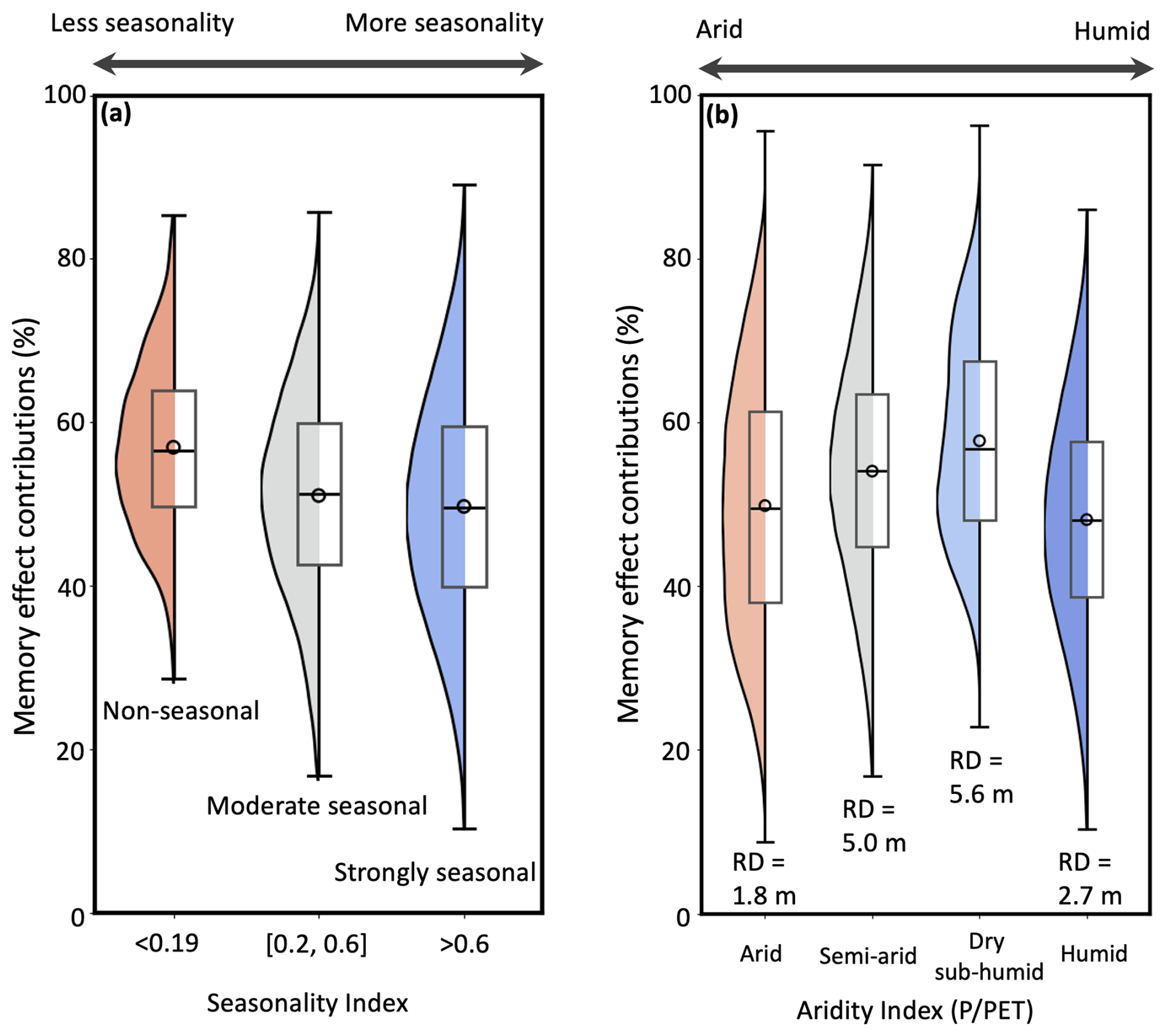
Figure 10 The Relationship Between Seasonality index, Aridity Index, and the Memory Effect as Captured by the Temporal Memory-Aware Model. The relationship between memory effect contributions to Evaporative Fraction predictions and the seasonality index (a), aridity index (b). In the box plots, the central lines represent the median values, the circle represent the mean values, the upper and lower box limits represent the 75th and 25th percentiles, and the upper and lower whiskers extend to 1.5 times the interquartile range, respectively. The violin plot shows the data points density distributions. The annual mean ratio of precipitation to potential evapotranspiration is used as an aridity index. Data sources include TerraClimate (for the aridity index calculation) via Google Earth Engine (Abatzoglou et al., 2018). The memory contribution metric uses the full dynamic predictor set, S= {P, Ta, RAD, VPD, WS, LAI}.

We further explored the hidden information within the memory effect contributions ($\sum _{-\mathrm{365}}^{-\mathrm{7}}\left|\mathrm{EG}\right|/\sum _{-\mathrm{365}}^{\mathrm{0}}\left|\mathrm{EG}\right|$) by examining its relationship with soil sand fraction (an indicator of soil matric suction and soil water holding capacity), rooting depth, seasonality index and the aridity index across different PFTs. Memory effect contributions increased with deeper plant rooting depths (Fig. 9a). Vegetation with deep roots, such as forests, showed a stronger memory effect, with contributions averaging up to 65 %, whereas shallow-rooted vegetation showed a weaker memory effect, with an average contribution of 45 %. Memory effect contributions also generally decreased with increasing soil sand fraction (Fig. 9b). In addition, memory effect contributions decreased with increasing seasonality index (Fig. 10a). Across aridity gradients, lower memory effect contributions were found in drier systems such as woody savannas, savannas, and open shrublands, with an average value of 49 % for aridity indices below 0.2, whereas wetter forest systems showed higher memory effect contributions, averaging 59 % (Fig. 10b). Overall, the results indicate that memory effect contributions vary systematically across vegetation and hydroclimatic gradients.

5 Discussion

5.1 Why Memory effect matters for EF dynamics predictions

The comparison with the benchmark models shows that explicitly accounting for memory effects is essential for accurately predicting EF dynamics. Across training strategies, vegetation groups, and hydrological conditions, the LSTM consistently outperformed the benchmark models, especially the climatology- and SPI-based models, which often yielded near-zero or negative NSE values. Even compared with the FNN, which used the same length of time-series input, the LSTM achieved higher predictive skill, indicating that the gain did not arise simply from the choice of input variables, but from the ability to represent temporal dependencies (Figs. 2, 3). This difference was particularly evident during drydown periods, when EF depends not only on concurrent forcing but also on antecedent hydroclimatic conditions. In particular, the poorer performance of the climatology- and SPI-based models reflects their inability to represent event-scale rain-pulse responses, post-rainfall EF decay, and the effects of antecedent hydroclimatic conditions on EF dynamics. Previous ML studies on ecosystem fluxes have mainly focused on GPP, NEE, or ET, often in the context of spatial upscaling (Besnard et al., 2019; Kraft et al., 2025; Montero et al., 2024; Biegel et al., 2025; Nakagawa et al., 2023). In contrast, EF is a normalized ratio variable, and our primary objective here is to understand temporal EF dynamics and memory effects rather than large-scale spatial transfer. This distinction is important because relatively simple radiation- or light-driven frameworks can already explain a substantial fraction of variability in ecosystem fluxes such as GPP (Stocker et al., 2020). Model performance should therefore be interpreted in the context of both the target variable and the evaluation setting. Accordingly, the strongest performance obtained under the time-based split should be interpreted as temporal generalization within sites rather than as evidence of strong transferability to unseen sites. The lower performance under site-based cross-validation and LOSO is consistent with the broader ecosystem-flux literature showing that spatial generalization remains more challenging than within-site temporal prediction.

Beyond its superior benchmark performance, the LSTM also reconstructs EF dynamics during soil moisture drydown periods, indicating that the model captures the key dynamics of post-rainfall water depletion (Fig. 4). Consistent improvements in model performance, particularly during drydown periods, indicate that incorporating memory enables the LSTM to better capture EF dynamics across temporal scales. These findings highlight the LSTM's strength as an explanatory model for EF dynamics, capable of capturing both short-term post-rain responses and background variability beyond what simpler models can achieve (Fig. 4). This underscores the importance of the memory effect and the superiority of the LSTM architecture in accurately predicting EF. The LSTM model, comprising input, forget, and output gates, manages to long-range retain or discard patterns in meteorological data, thereby capturing long-term dependencies effectively. Crucially, this mechanism is analogous to a water infiltration and retention in the soil and slow evapotranspiration processes, where prior rainfall is conserved as soil moisture and later accessed by plants' root systems for plant function and growth (Dralle et al., 2020). Consequently, our model can accurately simulate the physical process of plant water usage during dry spells and its time dependence as sketched in Fig. 1.

The event-level attribution patterns further suggest that antecedent precipitation plays a key role in sustaining EF during prolonged drydown periods, likely through its influence on soil water storage (Fig. 5). The EG contributions of VPD and vegetation conditions further indicate that atmospheric demand and plant status regulate how stored water is utilized. In addition, the delayed response to low-temperature events may reflect legacy effects of cold stress on vegetation functioning, highlighting the importance of climate memory in shaping EF dynamics across multiple temporal scales (Fig. 5).

These patterns are consistent with soil water processes in which wet-season precipitation supplies the initial water storage that is subsequently depleted through evapotranspiration during prolonged dry periods. EF therefore peaks after rain pulses and then gradually decreases at varying rates during drydown intervals, with the pace of decline reflecting differences in evaporative demand, rooting depth, and plant water-use strategies. For example, grasslands, with typically shallow roots, exhibit a faster EF decay compared to savannas, which suggest a deeper rooting system and/or lower canopy conductance for the latter (Fig. 4), consistent with in-situ observations (Dralle et al., 2020; Fan et al., 2017; Ichii et al., 2009; Seyfried and Wilcox, 2006). The investigations of the variations in EF decay rates offers a promising avenue for inferring rooting depths, and plant water-use strategies across sites and underscores EF's potential as an indicator of vegetation-regulated water stress responses. In forested systems, the observed variability is likely due to processes such as canopy interception (Lian et al., 2022). The differing rates of soil moisture dry-down among these sites likely reflect variation in plant rooting depths and water use strategies, which in turn influence the characteristic time scales of drought response.

Taken together, these findings underscore that memory effects are necessary for understanding and predicting EF dynamics, particularly under non-equilibrium conditions and across different plant functional types and site-specific settings, which are not adequately captured by the benchmark models. Incorporating memory effects therefore improves not only predictive performance, but also the ability to build an explanatory framework that better reflects the time-dependent nature of EF regulation.

5.2 Ecohydrological mechanisms and plant water-use strategies underlying Memory effects

The memory effects identified by the LSTM-based explanatory framework suggest that antecedent precipitation and temperature are key drivers shaping EF dynamics over extended timescales (Figs. 6, 7). Precipitation feeds the available water resources, i.e., root-zone soil layer, used to sustain the ecosystem during droughts. Air temperature and precipitation emerged as more dominant than radiation when memory effects are considered. Although radiation is a key driver of instantaneous evaporative demand through energy input, the LSTM model's ability to account for memory and legacy effects likely explains the elevated importance of temperature. We note, however, that air temperature and radiation are partly correlated, so their individual contributions should not be interpreted as fully independent. This suggests that while radiation influences short-term EF variation, air temperature plays a more critical role over longer timescales, highlighting the necessity of incorporating memory effects when predicting EF and related land-atmosphere fluxes. VPD provides a measure of atmospheric aridity, significantly affecting ET and thus EF. LAI did not emerge as a dominant feature for EF prediction, partly due to spatial and temporal discrepancies in the MODIS LAI product (250 m, 4-d) but also to the fact that most variability in EF at dry sites is due to soil moisture decay and driven by (lack of) precipitation. Cloud cover or aerosols may also contaminate the MODIS LAI data (Yang et al., 2006). Wind speed's minimal effect on EF predictions aligns with recent data-driven research (Gentine et al., 2011; Lhomme and Elguero, 1999; Zhao et al., 2019), showing that evapotranspiration is not strongly affected by wind speed, which is consistent with previous studies (Chen et al., 2018; Guérin et al., 2020).

Recent studies have also highlighted temperature-related memory – often referred to as heat stress (HS) memory – at the molecular scale, revealing mechanisms and regulatory layers involved in HS memory formation and resetting. These processes play a crucial role in enhancing plant stress resilience and fitness. During episodes of excessively high temperatures, plants can suffer cellular damage, primarily due to impaired photosynthesis and respiration, accumulation of misfolded proteins, and the production of reactive oxygen species. In natural environments, plants frequently encounter multiple recurring heat stress events rather than isolated incidents. The timing of these events can vary considerably, with subsequent extremes occurring shortly after or long after the initial one (Staacke et al., 2025). This variability can significantly influence vegetation functioning and transpiration – and thereby, evaporative fraction – at later stages. Moreover, the lag time of vegetation response to high temperatures is generally longer in mid- and high-latitude regions than in low-latitude ecosystems (Xiao et al., 2024). Forests, for instance, tend to initiate resistance mechanisms earlier due to their deeper rooting systems. However, once physiological functions are affected, forests are slower to recover (Xiao et al., 2024). In contrast, grasslands, though often more vulnerable to climate extremes, typically recover more quickly (Ying et al., 2020).

Overall, the differences in rooting depth and water-use strategies across vegetation types may create a trade-off between resistance and resilience, potentially leading to post-extreme spatial heterogeneity in vegetation responses. This underscores the importance of further investigating how such memory effects – especially temperature-induced – manifest across ecosystems and influence EF.

The learned memory effects appear to map onto key subsurface controls, particularly rooting depth and soil water-holding capacity (Figs. 8, 9). The faster decay of antecedent contributions in grasslands and the slower decay in shrub/savanna and forest systems are consistent with the idea that deeper-rooted vegetation can access water stored over longer periods, whereas shallow-rooted systems rely more strongly on recent precipitation. In this sense, the memory decay curves derived from EG provide a compact, process-relevant summary of how antecedent hydroclimatic information is retained in EF predictions across ecosystems. The positive biome-level relationships at selected quantiles between rooting depth and both t₅₀ and t₂₀ further support this interpretation, suggesting that slower memory decay can be associated with greater access to stored water. At the same time, the strength of the relationship varied across percentile aggregations, and substantial within-biome variability remained, indicating considerable uncertainty. Because the flux-derived memory metrics are ecosystem-scale whereas the Tumber-Dávila et al. (2022) rooting-depth observations are species-level and are not spatially matched, these grouped relationships should be interpreted as broad correlative indicators rather than site- or species-specific associations or direct quantitative estimates of rooting depth. This also suggests that rooting depth alone does not fully determine the learned memory timescales. Additionally, plant-available water storage is influenced not only by rooting depth but also by soil water holding capacity (Piedallu et al., 2011). In the field experiments, sandy soil was found to hold significantly less plant-available water per foot of soil compared to silt loam (Shwetha and Varija, 2015; Verheijen et al., 2019). In line with this, previous studies demonstrated that vegetation functioning during drought years in the Amazon rainforest is shaped by both rooting depth and water table depth (WTD) (Chen et al., 2024). Thus, incorporating reliable WTD datasets into future analyses could provide deeper insight into subsurface water access and its role in modulating vegetation responses and memory effects.

This interpretation is further supported by the relationships between memory effect contributions and soil sand fraction, seasonality index, and aridity index (Figs. 9 and 10). Our findings suggest that the memory effect contribution increases with deeper plant rooting depths. Vegetation with deep roots, such as forests, can access deep soil water storage derived from antecedent precipitation over longer periods, resulting in a stronger memory effect, averaging up to 65 % contribution. Conversely, vegetation with shallow roots relies more strongly on soil water stored in recent periods and therefore shows a weaker memory effect, with an average contribution of 45 % (Fig. 9). The relationship between memory effect and soil sand fraction is also consistent with this interpretation. Higher soil sand fractions correspond to a decreasing memory effect, likely because reduced soil suction and lower soil water-holding capacity limit the ability of soils to retain precipitation from antecedent periods. While there is a general monotonic decrease in the memory effect with increasing soil sand fraction, rooting depth remains a critical factor, with both rooting depth and soil properties jointly regulating plant water-use strategies. In addition, memory effect contributions generally decrease with increasing seasonality index, suggesting that ecosystems in highly seasonal climates rely more strongly on short-term rain pulses than on long-term antecedent storage (Fig. 10). Across aridity gradients, lower memory effect contributions in dry areas, such as woody savannas, savannas, and open shrublands, and stronger memory effects in wetter forests further support the idea that hydroclimatic setting, subsurface storage, and vegetation traits together shape the persistence of memory effects. In dry systems, shallow rooting depths and high soil sand fractions are associated with lower memory effect contributions, averaging 49 % for aridity indices below 0.2. In wetter systems, forests with deeper rooting depths and lower soil sand fractions are better able to utilize water stored from antecedent precipitation, resulting in higher memory effects, averaging 59 %. Notably, the persistence of strong memory effects even in humid forests suggests that rooting depth exerts an important control across climate regimes, rather than only in water-limited systems. Therefore, the memory effect captured here should be interpreted not as a direct one-to-one proxy for rooting depth, but as an integrated signature of plant water access, subsurface storage, hydroclimatic setting, and ecosystem-specific drought response timescales.

The learned memory effects also suggest clear seasonal differences in how antecedent climate influences EF dynamics and plant water-use strategies. The observed decrease in memory effect contributions with increasing seasonality index suggests that ecosystems in highly seasonal climates tend to rely more on short-term rain pulses and instantaneous climatic drivers rather than antecedent conditions. One possible explanation is that sharp dry-wet seasonal transitions shorten biologically active periods, thereby limiting the time window over which memory effects can persist. However, it is important to note that memory is often co-regulated by multiple climatic drivers, such as precipitation and temperature, and their interactions may vary across ecosystems. Therefore, further investigation is needed to fully understand the underlying mechanisms and to disentangle the role of seasonality in regulating memory effects.

The long duration of the learned precipitation memory further suggests that antecedent precipitation from different seasons may exert distinct legacy effects on plant water-use strategies. In our analysis, winter precipitation at DE-Obe and FR-Pue occurring close to 365 days earlier may continue to contribute to target-day EF predictions (Fig. S6). This observation aligns with the previous studies and experimental findings. For instance, antecedent winter precipitation from one or two years prior has been shown to influence growth in the current period (Bose et al., 2024; Kannenberg et al., 2020; Marqués et al., 2022; Shen et al., 2016). While legacy effects have been widely reported for winter precipitation in temperate ecosystems, similar effects may also result from summer precipitation in regions where it dominates annual rainfall (e.g., tropical zones or monsoonal regions). Further investigation at the seasonal and event scale is warranted to differentiate the contributions of summer versus winter precipitation memory. The contributions of the memory effect can also be observed for other variables, such as VPD, air temperature and radiation (Fig. 5). Therefore, we emphasize that ignoring the memory effect or legacy effect can introduce bias in detecting the main drivers and hinder a comprehensive understanding of key processes. Our framework provides event-level insights that can be leveraged to explore seasonal variations in ecosystem memory and the co-regulation of EF by multiple climate drivers. These insights lay the groundwork for future classification and clustering analyses aimed at characterizing diverse memory regimes across different climate contexts.

Taken together, these results suggest that EF dynamics and their associated memory effects can serve as emergent indicators of plant water-use strategies across ecosystems, consistent with our initial motivation in Fig. 1 to use fast and slow EF decay rates to infer differences in plant water access and drought-response behavior. However, these relationships should be interpreted as correlative indicators of apparent rooting-zone water storage capacity and plant water-use strategies, rather than as direct quantitative estimates of rooting depth, which would additionally require information on soil texture, groundwater constraints, and water consumption during dry-down.

6 Conclusions

In this study, we developed an explainable machine learning framework that incorporates the memory effects of meteorological drivers to better understand the mechanisms controlling evaporative fraction – a key indicator of plant water stress. The model was trained using eddy covariance data from the combined ICOS, AmeriFlux, and FLUXNET2015 Tier 1 datasets. Our main findings are as follows:

1. The LSTM model demonstrated strong performance across diverse plant functional types, outperforming all baseline models on test datasets.

2. The model adequately captures and reconstructs the EF dynamics, particularly during soil moisture dry-down periods very well and these observations are consistent with soil moisture decay patterns.

3. By accounting for the memory effect, air temperature and precipitation rather than radiation, emerged as the most influential driver of EF predictions, followed by VPD. Notably, the Expected Gradients' temporal analysis indicated that the model accounts for more historical time steps for forest and savanna sites compared to grassland sites, likely due to differences in vegetation rooting depths and water usage strategies. Our analysis suggests grassland sites generally rely on shorter time periods, spanning several months, for most of EF predictions.

4. Further investigation reveals that memory effect is closely associated with rooting depth, soil sand fractions, seasonality index, and aridity index. These findings highlight novel mechanisms that emerge only when the memory effect is considered. This underscores the potential of using the EF across diverse PFTs to reflect varying plant water stress conditions and water use strategies.

Our results highlight the importance of memory effects for interpreting EF dynamics and assessing ecosystem water stress. At the illustrated DE-Obe and FR-Pue sites, the model learned precipitation signals occurring nearly one year before the target dates, indicating potential long-duration associations that warrant further event-level investigation. Incorporating memory awareness into our modeling approach also offers opportunities to diagnose differences in apparent rooting-zone water storage and plant water-use strategies across biomes, an important but often overlooked aspect of land surface and Earth system modeling.