Technical note: A Water Analysis Trailer for Environmental Research (WATER)

In complex hydrological systems, flow path dynamics, water storage and mixing, and biogeochemical processing vary in space and may change rapidly during events. Understanding source areas, connectivity and short-term dynamics in stream water quality therefore requires high-temporal-frequency, multi-source observations both within and across catchments. Revolutions in field-deployable analysers and sensors, together with advancement in automation techniques, now make such observations feasible via true “labs-in-the-field”. This paper details the technical realisation and proof-of-concept for the Water Analysis Trailer for Environmental Research (WATER). The WATER is a mobile, trailer-based platform for environmental sensing and automated, high-temporal-frequency sampling and analysis of water from multiple (currently up to 11) sources. It offers two analytical pathways – a Throughflow Pathway for measurement devices using a flow cell and a 5 µm-filtered Reservoir Pathway for devices requiring filtered water – and is currently equipped to measure stable water isotopes, nitrate, electrical conductivity, pH and temperature. Integration of additional measurement devices in the future is supported by the modular design of the WATER. A field test in the 1.03 km² Schwingbach Environmental Observatory, Germany, demonstrated the ability of the system to successfully and autonomously collect and analyse samples from six water sources (2× stream water, 3× groundwater, 1× precipitation) over a period of six months, with collected data offering potential for new understanding of catchment functioning. Insights were also gained into the practical considerations necessary when deploying the WATER for an extended period of time, such as ensuring an adequate self-sufficient power supply and scheduling routine maintenance visits. Simulation of the reduced sampling frequency that would result from extending the WATER to sample at its full capacity of 11 sources also indicated that, over multi-month periods, key distributional characteristics of the collected data would likely be maintained. Overall, the WATER provides a mobile and scalable solution for high-temporal-frequency, multi-source hydrological and hydrochemical monitoring that can be (re-)deployed in different locations with relative ease.

1 Introduction

It has been known for some time that in order to understand the hydrological and hydrochemical functioning of a catchment, measurements pertaining to water quantity and quality must be made at the timescales relevant to the governing processes (Kirchner et al., 2004). As a result, significant advances have been made in the development of field-deployable analysers and sensors that permit in-situ, high-temporal-resolution measurements at a reasonable cost and without requiring the transport and analysis of water samples in a laboratory (Rode et al., 2016). For example, laser spectroscopes have been successfully adapted for use in the field (Berman et al., 2009; Pangle et al., 2013), and are capable of making quasi-continuous measurements of stable water isotopes when combined with a diffusive sampler to rapidly transform water from its liquid to vapour phase via diffusion across a porous membrane (Munksgaard et al., 2012). Meanwhile, UV hyperspectral spectrometers capable of measuring parameters such as nitrate (Sandford et al., 2007) and dissolved organic carbon (Sandford et al., 2010) at a very high temporal frequency, have helped increase the array of water quality parameters that can be measured in-situ beyond those possible with electrode-based sensors that have been available for decades (e.g., Carritt and Kanwisher, 1959). As reviewed by several recent papers (Benettin et al., 2022; Bieroza et al., 2023; Burns et al., 2019; Rode et al., 2016; Rozemeijer et al., 2025; van Geer et al., 2016), the revolution in high-temporal-frequency measurement devices has transformed – and will continue to transform – our ability to trace water fluxes through catchment systems, elucidate the sources and flow paths that contribute pollutants to rivers, improve estimation of pollutant loading, assess compliance with regulatory standards, develop and test new conceptual and numerical models, and inform appropriate catchment management strategies.

An emerging approach for combining multiple analytical and sensor technologies for longer-term, high-temporal-frequency measurements is the development of so-called “labs-in-the-field” – powered and fixed installations housing various measurement devices and some form of automated sample acquisition and delivery system. For example, von Freyberg et al. (2017) developed a lab with a dual-channel ion chromatograph (IC) and a diffusive sampler coupled to a cavity ring-down laser spectrometer to automatically measure major anions/cations and stable water isotopes in stream water or precipitation every 30 min. Meanwhile, Floury et al. (2017) developed the “River Lab”, which houses two ICs and several water quality probes to measure the hydrochemistry (anions, cations, pH, conductivity, dissolved oxygen, dissolved organic carbon, turbidity and temperature) of continuously pumped stream water every 30 to 40 min. Following the prototype, further River Labs have been customised and installed to sample rivers draining catchments up to 1500 km² in area (Brekenfeld et al., 2025). Both lab variants have successfully captured multi-parameter, high-temporal-frequency data for contrasting events occurring over an extended period of time, permitting new inferences to be made regarding catchment water storage and release (von Freyberg et al., 2017), the role of vertical connectivity in setting solute- and event-specific concentration-discharge relationships (Floury et al., 2024), and the disproportionate contribution of large storms to solute export (Wang et al., 2024).

As high-temporal-frequency analysis has become more common, it is increasingly recognised that continuing to advance our understanding of hydrological and hydrochemical processes requires monitoring to be extended from one or two stream water sources to spatially distributed sources within multiple catchment compartments (Bieroza et al., 2023). Such measurements can help identify longitudinal patterns of stream water chemistry which can be linked to in-stream processes or local solute sources (Winter et al., 2021), constrain the changing nature of lateral and vertical hydrological connectivity and solute distributions under contrasting hydroclimatic and antecedent conditions (Knapp et al., 2022), and overall reduce issues of process equifinality that can arise when drawing inferences from measurements taken from a limited number of in-stream locations (Knapp and Musolff, 2024). Furthermore, being able to gather similar measurements from a range of different catchments can enable hypotheses of catchment functioning to be tested in contrasting environments (Knapp et al., 2025). Heinz et al. (2014) designed and implemented a lab-in-the-field that permitted flexible and automated sampling of multiple water sources from a centralised location using one set of measurement devices. The system was successfully implemented in a rice paddy environment to measure stable water isotopes and nitrate in precipitation and irrigation water, as well as in 10 groundwater and ponded surface water sources located in fields experiencing contrasting management regimes. Each source could be sampled once every 6 h (Mahindawansha et al., 2018). However, this setup was again restricted to a fixed location and required a local power supply. Consequently, cross-catchment investigations would still require multiple instances of the lab-in-the-field to be installed at significant expense.

This paper reports on the development and testing of the Water Analysis Trailer for Environmental Research (WATER). The intended purpose of the WATER is to provide a mobile sampling platform capable of measuring the stable water isotope composition and water quality of multiple water sources distributed in space at a high temporal frequency. The next section outlines the design of the WATER, which builds on experiences made by Heinz et al. (2014) and Mahindawansha et al. (2018). A field test is then presented to provide a proof-of-concept for the WATER and highlight practical considerations for its operational use. Finally, the scalability of the WATER is assessed to understand the potential trade-offs between the number of water sources that are sampled, the temporal frequency of sampling, and the resultant distribution of collected data.

2 Design of the WATER

To fulfil its intended purpose, the design of the WATER needed to incorporate the following features:

• A mobile housing to facilitate deployment to a new location within a day.

• A self-sufficient power supply and automated security and fire suppression systems for deployment to remote areas.

• An automated sample acquisition and measurement system with a high throughput rate (maximum 20 min per sample) to enable high-temporal-frequency analysis of multiple water sources.

• Modular hardware and software constructions to offer flexibility in the measurement devices that can be installed.

• Remote software access to check system status, alarm messages and the sampling schedule.

• The ability to connect to local and remote sensor networks for the acquisition of complementary hydrometric data or to trigger sampling of specific water sources.

The following sub-sections outline and justify how these design criteria were met. The total cost of the WATER consists of approximately EUR 130 000 for the platform and EUR 180 000 for the measurement devices, resulting in a total cost that would be slightly under EUR 310 000 as of 2025 (see Sect. S1 for a full cost breakdown).

2.1 Trailer and basic infrastructure

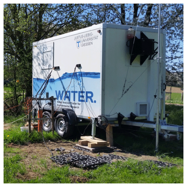
The basis of the WATER is a custom-made closed trailer with an insulated shell and integrated furniture. A trailer was chosen over a dedicated vehicle to optimise the balance between mobility and costs. The insulated shell of the trailer helps to buffer daily and seasonal temperature fluctuations. There are also systems that can provide additional heating or cooling, depending on specific conditions. If the temperature inside the trailer becomes too high (low) whilst the outside temperature is cooler (warmer), a passive ventilation system (EAT 6 G/1, Maico Elektroapparate-Fabrik GmbH, Villingen-Schwenningen, Germany) draws in the cooler (warmer) air from outside to adjust the internal temperature to within ±5 °C of a set temperature. Meanwhile, if the internal temperature is too low whilst the outside temperature is also cooler, a diesel heater (Air Top Evo 40, Webasto SE, Stockdorf, Germany) becomes active to provide additional warming. The only scenario where further temperature regulation is not possible is when the internal temperature of the trailer is too high and the outside temperature is warmer still. To mitigate this issue for particularly temperature-sensitive measurement devices, a fully climate-controlled server enclosure (TS IT 5528.129, Rittal GmbH & Co. KG, Herborn, Germany) with two thermoelectric coolers (SK 3201300, Rittal GmbH & Co. KG, Herborn, Germany) is available, offering heating and cooling to within ±1 °C of a specified temperature for ambient temperatures between −30 and 55 °C.

Power to the trailer can be provided by solar panels connected to two 12 V 300 Ah batteries, a 5.1 kW diesel generator (5000i, Fischer Panda GmbH, Paderborn, Germany), or mains (grid) AC power. Three solar panels (SPM190-24/3a, Victron Energy, Almere, The Netherlands) with a combined peak output of 570 W are fixed to the top of the trailer. Additional free-standing panels can also be connected, with experience showing that a further six panels (additional peak output of 1140 W) can permit the WATER to be almost completely sustained by solar power in summer months with the current measurement device setup. Whilst relying on solar energy is more sustainable, it requires an open site for installation and is sensitive to sunlight availability. In addition, careful planning is needed to ensure that the power generated by the solar panels can meet the requirements of the measurement devices installed in the WATER. By contrast, the diesel generator offers a rapid, ready-to-use power supply that can provide a consistent high-power output whilst maintaining mobility. Power within the trailer can be supplied at 12 and 24 V DC, as well as by converted 230 V AC. For security purposes, the trailer is fitted with an alarm system and video surveillance. A fire suppression system using heptafluoropropane (HFC227) is also installed for the whole trailer, with a further dedicated system installed within the server enclosure. GPS tracking and a GSM modem are provided via a Mobile Autonomous Java Application device (MAJA, YAWiD Electronics GmbH Gröbenzell, Germany). The modem also facilitates the sending of system alerts via SMS text and email, as well as remote access to the WATER.

2.2 Sample acquisition system

A diagram of the sample acquisition system is provided by Fig. 1a. A peristaltic pump (P1; M1500, Verder GmbH, Haan, Germany) draws water from a source connected to an open valve within a valve array. The number of possible input sources is determined by the size of the valve array. The current setup provides 12 valves, one of which is used for maintenance. Consequently, 11 valves can be connected to external water sources via a sampling line, permitting analysis of multiple source types distributed in space. The sampling line should be made of an inert material (e.g., polyethylene) to be consistent with the internal tubing of the WATER and facilitate the full range of hydrological and hydrochemical analyses. The maximum horizontal distance to a source depends on whether the time needed to flush the sampling line (a function of the hydraulic properties of the sampling line and power of the peristaltic pump), can be accommodated by the sample throughput time. The vertical distance additionally depends on the hydraulic gradient. In the proof-of-concept application, maximum horizontal and vertical distances of approximately 145 and 3 m, respectively, were successfully achieved (see Sect. 3.1).

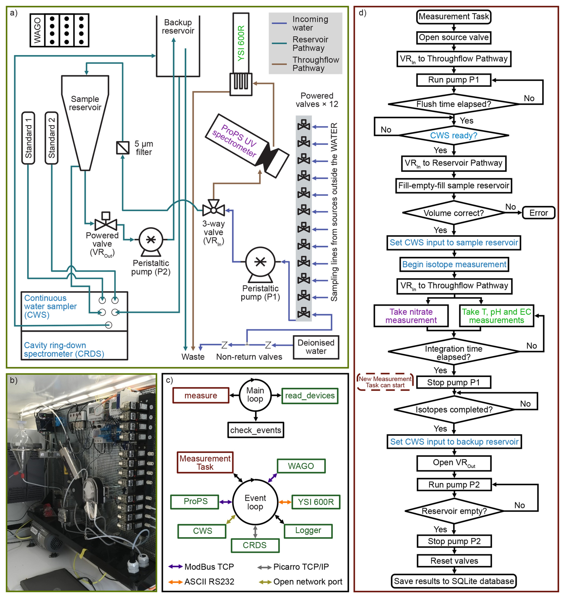
Figure 1 (a) Schematic of the automated sample acquisition and measurement system in the WATER; (b) photo of the valve and pump system, ProPS, YSI600R and sample reservoir; (c) schematic of the main software loop and event loop (coloured arrows in the latter denote the method of interfacing with devices whilst a black arrow indicates a software connection); (d) flow chart for a Measurement Task (coloured text denotes the device used in measurement acquisition and corresponds to device labelling in a).

A water sample is pumped either along the “Throughflow Pathway” or “Reservoir Pathway”. The pathway is determined by a 3-way valve (VR_In). The two pathways allow integration of measurement devices that require a continuous throughflow of unfiltered water or filtered water drawn from a reservoir, respectively. Water directed along the Reservoir Pathway is passed through a 5 µm filter before being received by a 1000 mL sample reservoir connected to a 5 kg load cell (SP4M-series, Hottinger Brüel & Kjaer GmbH, Darmstadt, Germany) used to measure sample volume. A 5 µm filter was used here as a trade-off between the required filter replacement frequency due to sediment accumulation and the need to remove particulates from the water sampled by the Continuous Water Sampler (CWS) during stable water isotope analysis (see Sect. 2.3). Filtering serves only to protect the membrane cassette of the CWS and has no effect on the isotopic signature of the water. If required by other measurement devices, alternative filter sizes could also be accommodated. A powered valve (VR_Out) and second peristaltic pump (P2; CP83, Gemke Technik GmbH, Ennepetal, Germany) are used to empty the sample reservoir into a backup reservoir, which in turn drains under gravity to the waste outlet of the WATER once it reaches a certain fill level. A 10 L container of deionised water is also connected to the system for rinsing purposes.

The valves, pumps and load cell are controlled by a WAGO programmable logic controller (PLC) with 32 digital outputs, 8 digital inputs and 12 analogue inputs (WAGO I/O system 750, WAGO Kontakttechnik GmbH, Minden, Germany). Also connected to the WAGO are two leak sensors that are placed beneath the sampling board to halt sampling and measurement should a water leak be detected. A central controller PC (NISE 101, NEXCOM Int. Co., New Taipei City, Taiwan), with a GNU-Linux operating system communicates commands to the PLC using self-developed software (see Sect. 2.4).

2.3 Measurement devices

The WATER is able to support measurement devices via the PLC or the Linux control computer. The latter supports multiple communication protocols (e.g., Modbus TCP/RTU, SDI-12, TCP/IP) and physical or wireless standards (e.g., RS232/485, ethernet, radio telemetry). Devices may be used directly in the analysis of a water sample, to trigger event-based sampling (see Sect. 2.4.1), or to collect ancillary environmental data. The latter, along with non-measurement devices related to the security of the trailer, are handled via a virtual logger device.

Figure 1a–b shows the configuration of the sample acquisition system and measurement devices in the current setup of the WATER. A YSI 600R multi-parameter probe (YSI Inc., Yellow Springs, USA) and a ProPS UV spectrometer connected to a TriBox2 measurement and control system (TriOS GmbH, Rastede, Germany) are available to make water quality measurements. The YSI 600R can measure electrical conductivity (EC), pH and water temperature, whilst the ProPS currently measures nitrate (NO₃-N); measurement of nitrite (NO₂) and organic content (chemical and biological oxygen demand; dissolved and total organic carbon) would also be possible. Both devices are configured with a flow cell and incorporated into the Throughflow Pathway. A Continuous Water Sampler (CWS; A0217, Picarro Inc., Santa Clara, USA), connected to a wavelength-scanned Cavity Ring-Down Spectrometer (CRDS; L2130-i, Picarro Inc., Santa Clara, USA), is available to measure the stable water isotope (deuterium and oxygen-18) composition of a sample. Measurements are reported in δ notation (δ²H and δ¹⁸O) relative to Vienna Standard Mean Ocean Water (VSMOW). The CWS is based on the diffusion sampling system of Munksgaard et al. (2011) and permits quasi-continuous measurement of stable water isotopes from liquid water. Standards with a known isotopic composition are required to correct for drift caused by the CWS (e.g., due to biofilm accumulation in the membrane) and CRDS. The CWS is part of the Reservoir Pathway, with one of its four inlets connected to the sample reservoir. Water is drawn into the CWS via a built-in solenoid diaphragm pump at a rate of 1 mL min⁻¹. Additional reservoirs containing isotopically heavy (+3.13 ‰ for δ¹⁸O and −1.52 ‰ for δ²H) and light (−22.43 ‰ for δ¹⁸O and −164.60 ‰ for δ²H) in-house standard water are installed at the same height as the sample reservoir, and each is connected to an inlet of the CWS. Ensuring a consistent height of all reservoirs is necessary as the height of a reservoir above the waste outlet of a CWS has been shown to affect measured isotope values (von Freyberg et al., 2017). The waste outlet is connected to the backup reservoir. The final inlet of the CWS is also connected to the backup reservoir so that a source of water should always be available to prevent the sampler from running dry.

2.4 Software

The WATER is largely controlled via high-level software written in Python running on the Linux control PC, though a separate program running on the WAGO PLC interacts with the valves, pumps and other hardware of the sample acquisition system. Both pieces of software are self-developed.

2.4.1 High-level software

The high-level software (Kraft et al., 2026) interfaces with all installed measurement devices, manages sample scheduling, acquisition and measurement, handles local data storage, facilitates remote access, and monitors the overall status (e.g., security alerts, fuel warnings, etc.) of the WATER. The code is open source, uses a free software stack, and is designed to be extendable (e.g., to incorporate additional measurement devices). The setup of the WATER is defined by a sampler configuration file and a schedule file, both in YAML format, that are read in by the software when first executed. The software also launches a web app where additional setup information can be provided, and sampling can be commenced (Fig. 2). The configuration file specifies global system parameters (e.g., device read rate, sample volume, and various software timeouts), along with a list of measurement devices connected to the WATER. For each device, an additional Python file is required that specifies the unique functions of the device needed for sample analysis. The schedule defines the sequence in which sources should be routinely sampled and any events that should trigger sampling of a specific source. Sources are identified by their IDs in the valve array (Fig. 1a). The web app is then used to link valve IDs to the attributes of each source, including a name for the source, the flush time, and any additional comments. Trigger events can be defined based on threshold measurements set for ancillary measurement devices connected to the WATER, such as rainfall collectors, soil moisture sensors and groundwater level loggers. Multiple triggers can be incorporated within one schedule. The schedule and relevant sources can be edited after deployment of the WATER via the web app (Fig. 2b), which also displays information about measurement and device statuses, system logs, and past and future sample processing (Fig. 2a).

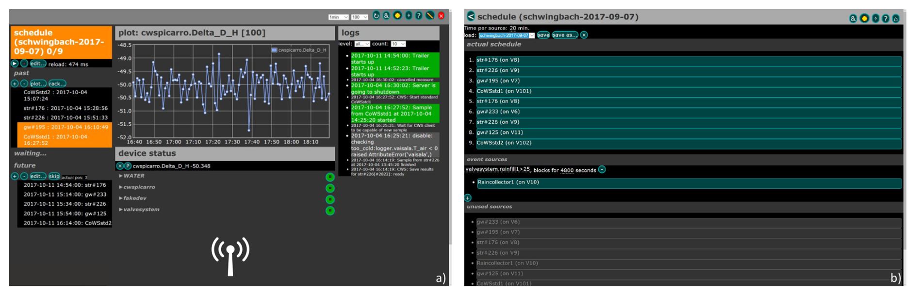
Figure 2 (a) The dashboard of the web user interface for the WATER, showing the past and future sampling schedule, measured data and the system log; (b) the sample schedule, consisting of routine and event-triggered samples.

After setup and sampling commencement, the main software loop runs continuously whilst the WATER is active and repeatedly calls three functions: read_devices, check_events and measure (Fig. 1c). The first function updates the status of all connected devices, logs any errors, and deactivates any device that is consistently unresponsive. The second checks whether any of the specified conditions for event-triggered sampling have been met and, if so, inserts the relevant source as the next source in the sampling schedule. The third begins a new “Measurement Task” (see Sect. 2.5) when the next source is due in the sampling schedule. The main loop relies heavily on the built-in Python package asyncio to facilitate asynchronous execution of functions (i.e., new functions can start whilst running functions are waiting for something to happen) submitted to an Event Loop (Fig. 1c).

Measurement data are stored in an SQLite database. The SQLite engine is integrated directly into the software. The database is primarily organised around a table of water sources, with each source having a table of samples and each sample having a table of measurements. Timestamping is applied at the sample level and reflects the time at which the fill-empty-fill routine for the sample reservoir was successfully completed (see Sect. 2.5). Therefore, all measurements for a sample are associated with the same timestamp. The database also contains tables for logging measurement processes, errors and system alerts. Critical system alerts (e.g., security issues, low diesel fuel level or equipment failures), cause SMS text and email notifications to be sent to a defined list of persons responsible for the WATER so that they can respond immediately to any problems and, thus, minimise potential data loss. To reduce the risk of acquisition and measurement errors during freezing conditions, the WATER pauses all sampling if ambient temperatures fall below 0 °C.

2.4.2 PLC software

The software for the WAGO PLC covers the basic functions of water flow through the sample acquisition system: flush sample line, fill sample reservoir, empty sample reservoir, and clean filter. Each function has a pre-programmed timeout and other error conditions to prevent damages by continuous running water if the connection between the high-level software and the PLC is lost due to either hardware or software failures. The high-level software activates the PLC functions over a ModBus TCP interface. The PLC software also provides additional functionality like reading and filtering analogue signals from the load cell of the sample reservoir and monitoring the temperature in/outside of the WATER. The system is programmed in CODESYS 2.3.9, partly by using the graphical programming language Functional Block Design (FBD) and partly by Structured Text (ST). The CODESYS 2.3.9 project is published as a CODESYS-XML file (Kraft, 2026).

2.5 Measurement Task

With the current hardware and measurement device setup, a Measurement Task initiated by the high-level control software proceeds as shown in Fig. 1d. It should be noted that a new Measurement Task can begin whilst the stable water isotope measurements for the current sample are still in progress. This allows for advanced flushing of the sampling line for the next sample so that new water is available to the measurement devices as soon as the sample is due. When a task begins, the required source valve is opened and VR_In is set to the Throughflow Pathway. P1 then starts running to flush the external sampling line. The flush time is set for each source separately based on an assigned flow rate and the volume of water in the line (dependent on length and diameter). For example, a 50 m line with an inner diameter of 4 mm would hold 630 mL of water. To flush the line twice with a flow rate of 500 mL min⁻¹ would require 2.5 min. If the stable water isotope measurements from the previous sample completed whilst the sampling line was being flushed, the Measurement Task continues; otherwise, it waits for the measurement to complete. VR_In is next set to the Reservoir Pathway so that the sample reservoir can be filled. To minimise carry-over effects between samples, the reservoir is rinsed with 60 mL of sample water, emptied, and then refilled with a further 60 mL of water (fill-empty-fill). Assuming again a flow rate of 500 mL min⁻¹ and accounting for necessary valve switching, this fill-empty-fill sequence would take approximately a further 25–30 s after flushing. If the load cell does not detect any water in the reservoir (e.g., due to clogging of a sample line or a source running dry), an error is raised and the Measurement Task ends. Otherwise, stable water isotope analysis with the CWS/CRDS begins. The CWS samples water from the reservoir for 20 min. This allows ample time for measurements to stabilise between samples (∼ 10 min), with the final isotopic composition of a sample recorded as the average measurement over the last 3 min of analysis.

Whilst the stable water isotope analysis is in progress, VR_In switches to the Throughflow Pathway and water is passed through the YSI 600R and ProPS for water quality analysis. For parameters measured by the YSI 600R, values are averaged over an integration period of 20 s. Meanwhile, to conserve the deuterium lamp of the ProPS, a single absorption measurement is made as water passes through the flow cell. Once the water quality measurements have been made, P1 stops. While the system waits for the stable water isotope measurements to finish, a new Measurement Task can start flushing the sampling line of the next sample. On completion of the isotope measurements, VR_Out opens and P2 empties the sample reservoir into the backup reservoir. The input of the CWS is also set to the backup reservoir so that it does not run dry whilst the next sample is acquired. All valves are then reset, and the measurement data saved to the SQLite database.

The total time for the analysis of one water sample is 20 min, set by the time required for the stable water isotope measurements to complete. With this sampling resolution, the WATER can analyse 72 samples per day. At least once every 6 h, material accumulated on the face of the 5 µm filter is dislodged by filling the sample reservoir with deionised water from the 10 L container and then reversing the direction of P1 to draw water back through the filter and to the waste outlet of the WATER.

2.6 Adding or changing water sources and measurement devices

Once the appropriate sampling lines have been connected or rerouted from the WATER, adding or changing water sources simply requires updating the schedule to reflect any changes in the valve IDs that are to be sampled, and the source attributes (e.g., flush time) to account for the new location of the source. Both tasks can be achieved remotely using the web app. For measurement devices, it would be necessary to update the list of connected devices in the configuration file of the WATER. If adding a new device, a Python file detailing the specific measurement functions of the device would also need to be provided. Calls to measurement devices in the relevant code for a Measurement Task would then have to be updated in the high-level software to reflect the changes. In general, no changes would be necessary to the PLC software unless modifying the sample acquisition system or connecting additional analogue devices (e.g., a tank electrode – see Sect. 3.1) to the WATER.

3 Field testing of the WATER

To provide a proof-of-concept and elucidate the practical considerations necessary for successful operation, a six-month (12 April to 11 October 2019) field deployment of the WATER to the headwater catchment of the Schwingbach Environmental Observatory (SEO) in Hesse, Germany (Fig. 3) was undertaken.

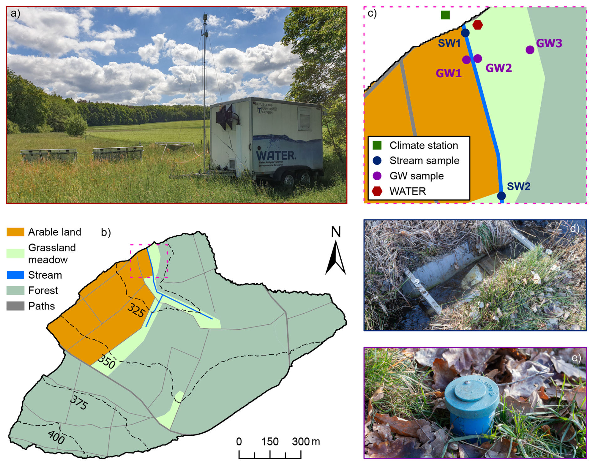
Figure 3 (a) The WATER positioned at the outlet of the Schwingbach catchment together with the precipitation collector and solar panels; (b) a map of the Schwingbach catchment showing the main land covers and elevation contours; (c) a map showing the location of the WATER (and precipitation collector) and sampled sources around the catchment outlet (extent is given by the dashed pink box in b); (d) an example of a sampled stream water (SW) source; (e) an example of a sampled groundwater (GW) source. Land cover data: © GeoBasis-DE/BKG 2018.

3.1 Catchment characteristics and setup of the WATER

The major land covers (Fig. 3b–c) of the 1.03 km² catchment area are forest (76 %), arable land (15 %) and grassland meadows (7 %). The latter mainly border arable land and the perennial Schwingbach stream. Cambisols and Stagnsols are the main soil types under forested and arable land, respectively. Elevation ranges from 310 m.a.s.l. at the outlet to 415 m.a.s.l. in the south-west of the catchment. The climate is temperate oceanic (Köppen climate classification). An automatic climate station (AQ5, Campbell Scientific Inc., Shepshed, UK) is located just outside the catchment boundary (Fig. 3c) and records climatic variables at 5 min intervals. Stream discharge at the outlet is derived at 10 min intervals using an RBC flume (Eijkelkamp Agrisearch Equipment, Giesbeek, Netherlands) equipped with a micro-diver pressure transducer (Eigenbrodt Inc., Königsmoor, Germany), and a calibrated stage-discharge rating curve for the flume provided by the manufacturer.

The WATER was positioned close to the outlet of the catchment (Fig. 3a and c). In addition to the three rooftop solar panels, a further six panels were connected to the trailer, providing a combined peak output of 1.7 kW. The power demand from the WATER was expected to be between 450 and 575 W, depending on the need for interior cooling. Supplementary power was available from the diesel generator when necessary. Six external water sources were connected to the WATER for sampling: two stream water sources (SW1-2), three shallow groundwater sources (GW1-3), and a precipitation source (Fig. 3c). SW1 was located at the catchment outlet, whilst SW2 was approximately 145 m upstream at the edge of the arable land. Each groundwater source was sampled from a piezometer made from a perforated PVC tube sealed with bentonite clay to prevent ingress of surface water. Samples could be drawn up from a depth of 3 m by the peristaltic pump (P1) of the WATER, with no additional pumps installed at the piezometers themselves. GW1 and GW2 were located either side of the stream under arable land and grassland meadow, respectively. GW3 was positioned further upslope at the edge of the forest. Precipitation was collected via a 3.3 m² funnel-type tarp connected to a 5 L bucket. A tank electrode (Votronic GmbH, Lauterbach, Germany) installed in the bucket and connected to the WAGO PLC triggered event-based sampling of precipitation based on accumulated depth.

The 72 daily samples that can be analysed by the WATER were distributed as follows. In the case of no precipitation, 16 samples would be analysed from each stream water source (n=32), eight from each groundwater source (n=24), and eight from each stable water isotope standard (n=16). If precipitation did occur, then an event sample would be taken whenever the accumulated depth in the collection bucket exceeded 0.3 mm. To avoid carry-over effects, the bucket was emptied after sampling had taken place, and the precipitation source blocked from the sampling schedule for 60 min to allow other sources to be sampled in the event of continuous precipitation.

3.2 Performance of the WATER

Over the six-month field test, the WATER automatically collected and analysed over 4000 surface water, groundwater and precipitation samples (Neill et al., 2026). Figure 4 presents precipitation and stream discharge during the field deployment, together with deuterium (δ²H), nitrate (NO₃-N) and electrical conductivity (EC) data for each source connected to the WATER. To better illustrate the high-temporal-resolution characteristics of the data, Fig. 5 presents the same data series but focused on a dynamic phase of catchment re-wetting, from 1 October 2019 00:00 CET (UTC+1) to 3 October 2019 12:00 CET (“focused period”). During this period, 12.8 mm of precipitation falling over a period of approximately three hours caused a clear peak in discharge of 1.7 L s⁻¹ (Fig. 5a).

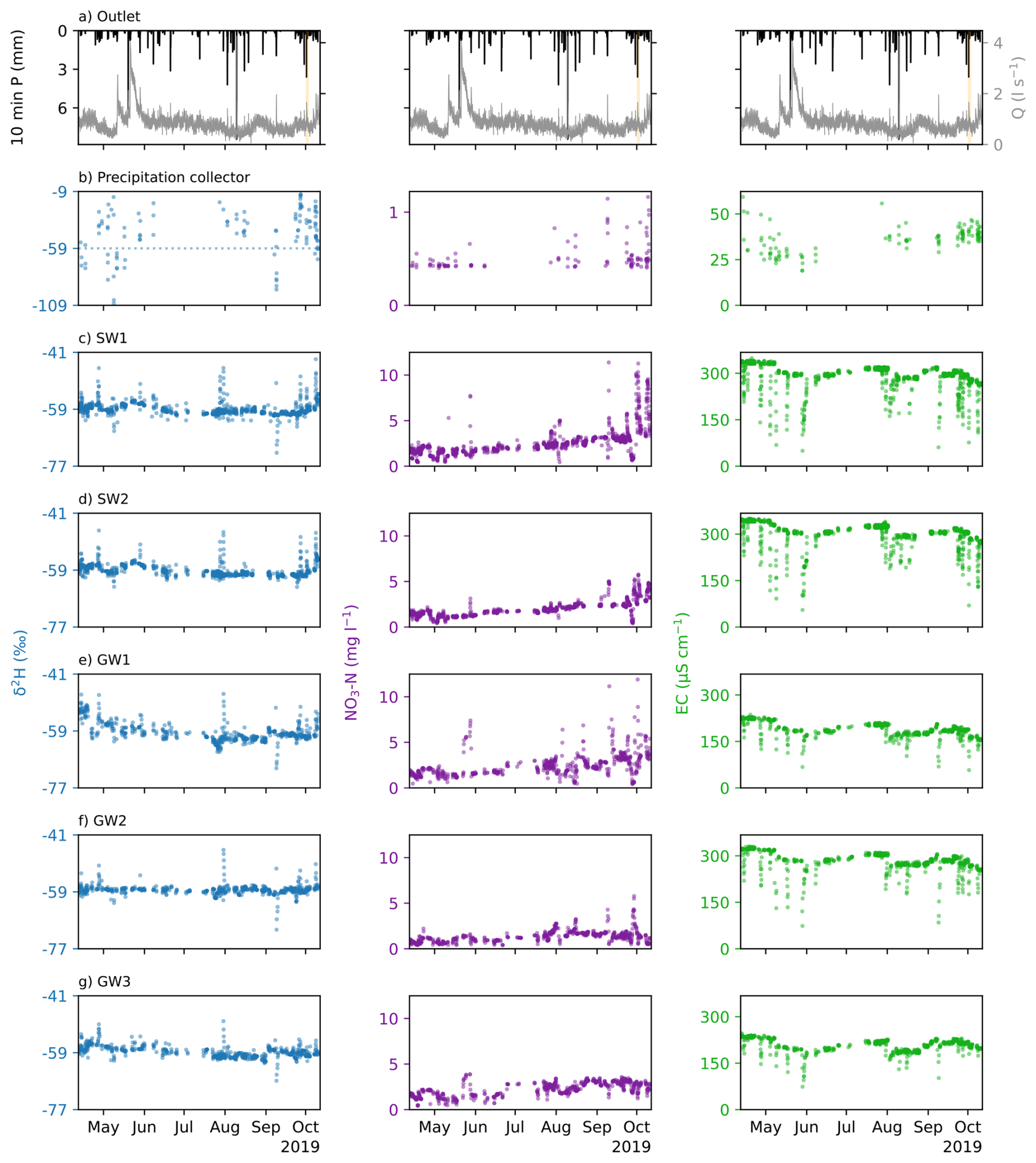
Figure 4 (a) Stream discharge at the catchment outlet and precipitation measured at the nearby climate station; and deuterium (δ²H), nitrate (NO₃-N) and electrical conductivity (EC) measurements for (b) precipitation water, (c) SW1, (d) SW2, (e) GW1, (f) GW2, (g) GW3. Note that precipitation water uses a different scale for all parameters relative to SW and GW sources. All δ²H sub-plots are centred on the mean value for all non-precipitation sources (shown by a dashed line in b). Data are presented for the full field test.

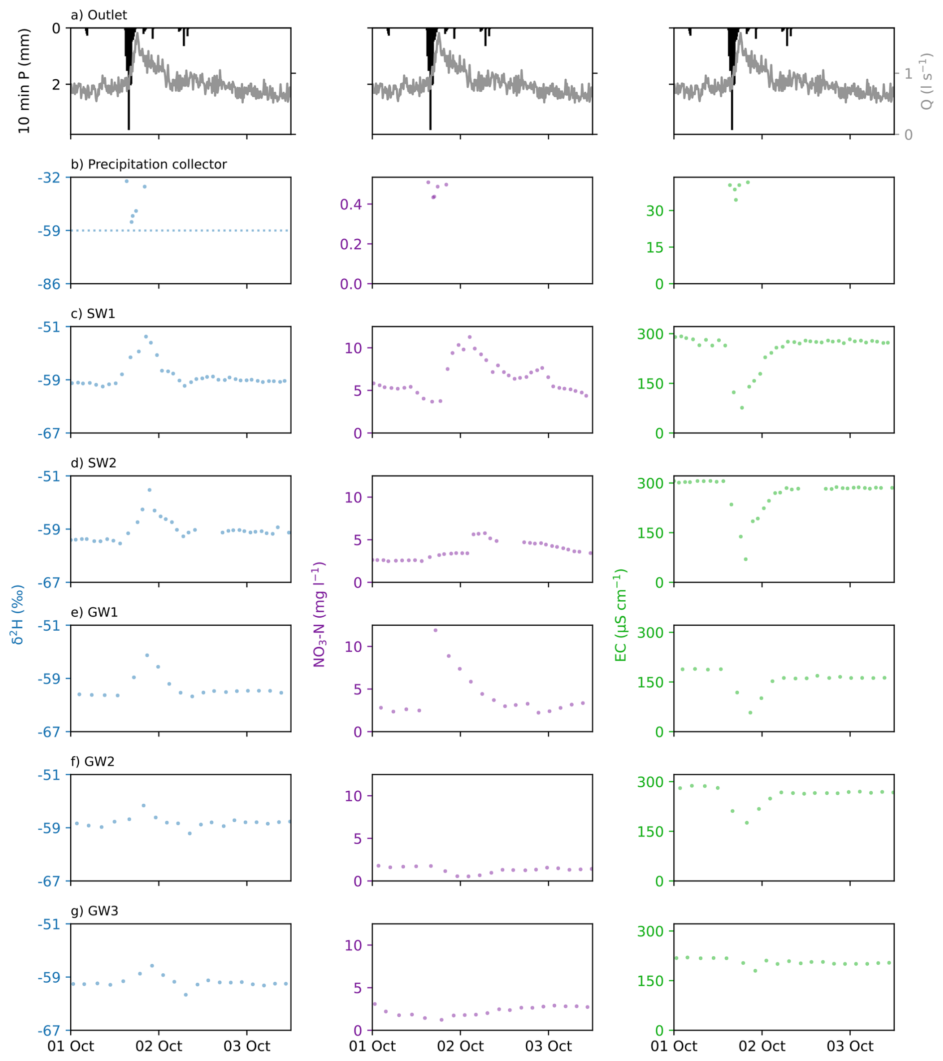
Figure 5 (a) Stream discharge at the catchment outlet and precipitation measured at the nearby climate station; and deuterium (δ²H), nitrate (NO₃-N) and electrical conductivity (EC) measurements for (b) precipitation water, (c) SW1, (d) SW2, (e) GW1, (f) GW2, (g) GW3. Note that precipitation water uses a different scale for all parameters relative to SW and GW sources. All δ²H sub-plots are centred on the mean value for all non-precipitation sources (shown by a dashed line in b). Data are presented for the focused period (1 October 2019 00:00 CET to 3 October 2019 12:00 CET).

Sampling and analysis of precipitation by the WATER could generally be successfully triggered based on the depth of water in the precipitation collector, though temporary issues with the tank electrode and funnel tarp did lead to some precipitation events being missed. Whilst the magnitude and variability of NO₃-N and EC in precipitation were minimal, the data collected by the WATER characterised substantial event-scale variability in δ²H (Fig. 4b). For instance, δ²H measurements from the main 3 h precipitation event in the focused period varied between −54.7 ‰ and −34.0 ‰ (Fig. 5b). The flexibility of the control software allowed precipitation sampling to be triggered at a sufficient frequency to capture such variability, despite the WATER also being connected to multiple surface and groundwater sources. Indeed, the sampling frequency of precipitation was comparable to the lab-in-the-field of von Freyberg et al. (2017), which sampled only a single stream water source in addition to precipitation. It would also be possible to prioritise other sources over precipitation (or other event-triggered sources) in applications where variability in the parameters of interest is expected to be low.

The WATER was also able to successfully sample multiple, spatially distributed stream and groundwater sources at a high-temporal-frequency for an extended period (Fig. 4c–g). Source-specific data gaps usually reflected unavailability of a source (e.g., due to groundwater levels falling below the depth of the sampling line), or temporary obstructions in the sampling line. The data collected by the WATER revealed both common and unique characteristics of the sampled sources, from which insights into the hydrological and hydrochemical functioning of the catchment can be gained. For instance, whilst the δ²H signal at all SW and GW sites was damped relative to measured precipitation (Fig. 4b–g), all sites could show deviations in the direction of the precipitation signal during events (Fig. 5b–g). A similar responsiveness was also observed in EC measurements. This implies a rapid vertical movement of incoming precipitation into shallow groundwater and the importance of shallow sub-surface flow paths in delivering water to the stream (Sahraei et al., 2020), catchment processes unresolved by previous studies that utilised weekly stable water isotope data (Orlowski et al., 2016).

Additionally, despite a separation distance of only 145 m (Fig. 3c), NO₃-N dynamics at SW2 and SW1 were markedly different. Instead, the latter showed greater synchronicity in terms of magnitude and response timing with GW1 (Figs. 4c and e; 5c and e), likely indicating the vertical leaching and subsequent lateral transfer of nitrate in fertiliser applied to the arable land between SW1 and SW2 (Fig. 3b). Data collection over several events also revealed that the relative timing of the response at SW1 and GW1 was not consistent (Fig. 4c and e), potentially reflecting changes in the spatio-temporal distribution of solute sources and their connectivity to the stream under various hydroclimatic and antecedent conditions (Floury et al., 2024; Knapp et al., 2022; Li et al., 2024). Such observations demonstrate the value of the spatially distributed data collected by the WATER in unravelling the confounding influences of upstream versus localised controls on stream water quality, and how these change over time (Bieroza et al., 2023).

Overall, the results from the field test provide a successful proof-of-concept for the WATER, both with respect to the ability of the system to automatically collect and analyse samples from multiple water sources at a high temporal frequency, and the potential value of the collected data in advancing understanding of hydrological and hydrochemical processes.

3.3 Considerations when operating the WATER

Despite being mobile, the WATER is still a laboratory utilising complex measurement devices whilst operating in the natural environment. Consequently, there is a need for routine maintenance tasks to be carried out. These include cleaning and calibrating the sensors of the YSI 600R and ProPS UV spectrometer, refilling the standard water reservoirs (ca. 5 L per month) and regenerating the Drierite air column for the CWS, ensuring the sampling lines are clean and free of obstruction, and replacing the 5 µm filter on the Reservoir Pathway. Experience from the field test showed that at least weekly maintenance was required, with shorter intervals being necessary if the sampled water was especially laden with sediment (e.g., due to high flow events). This frequency of maintenance is comparable to other lab-in-the-field setups (Brekenfeld et al., 2025; von Freyberg et al., 2017). For longer-term (>1 year) deployment of the WATER, additional maintenance considerations would be statutory roadworthiness testing for the trailer and the potential replacement of wear parts within measurement devices (e.g., the membrane cassette for the CWS).

The biggest consideration for the WATER is ensuring there is a sufficient, consistent power supply for the measurement devices. Despite the power rating of the solar panels installed for the field test substantially exceeding the requirements of the measurement devices, it was often necessary for supplementary power to be provided from the diesel generator. In addition, the two larger data gaps during the field test in June and July (Fig. 4) reflect more significant issues with the power supply system that required repair at a workshop, including a deep discharge of the battery pack due to a manufacturing error and a complete failure of the diesel generator. Whilst these failures are unlikely to be a recurrent issue, they do highlight the vulnerability of the WATER to power supply issues. Therefore, whilst it is reasonable to expect that the WATER can be sustained by a combination of solar and diesel power over a period of a few months, longer deployments would likely benefit from the availability of a mains power supply.

To provide an indication of the costs associated with a deployment of the WATER, average monthly operational costs in the SEO were estimated as EUR 208 over an entire year, EUR 283 for months requiring heating, and EUR 143 for months requiring cooling. Differences between each estimate reflect changes in the power demand from the WATER, the availability of solar power throughout the year, and the consequent usage of diesel to run the backup generator. Also included in each estimate were consistent monthly costs (e.g., for weekly replacement of the 5 µm filter), as well as proportional contributions to the costs associated with longer-term (>1 year) deployments of the WATER. More details are given in Sect. S2.

4 Scalability of the WATER

A major advantage of the WATER is that the sample acquisition system and self-developed software provide significant flexibility in terms of how many water sources are sampled and at what frequency. However, since samples are processed sequentially, a trade-off exists between the number of connected sources and the maximum possible sampling frequency of each source. To gain insight into how this affects the scalability of the WATER, data from the field test (hereafter the Baseline scenario) were sub-sampled to simulate the reduced sampling frequency that would result if the number of connected SW and GW sources was doubled. In this scenario (hereafter S1), all 11 inputs to the WATER would be in use (SW × 4, GW × 6, Precipitation × 1). It was assumed that the relative sampling frequency of SW and GW sources would remain consistent with the Baseline (i.e., 2:1). Precipitation was still considered to be an event-triggered source, with sampling occurring at the same frequency as in the Baseline. It was also required that the two isotope standards each still be sampled eight times per day. Under these conditions, sub-sampling simply involved retaining every other Baseline sample for each source. Datasets for δ²H, NO₃-N and EC were then generated using the measurements associated with the retained samples. To compare how the two different sampling configurations of the WATER compared to more traditional approaches, the Baseline data were also sub-sampled to simulate a Daily sampling strategy, with one sample collected per day per source between the hours of 1200 and 1500. This timeframe is representative of an automatic sampler being triggered in the early afternoon to minimise malfunctions due to freezing conditions that may occur in winter. Sub-sampling was achieved by generally retaining the first available sample for each day and source that was collected after 1200 but before 1500. However, if the first sample was missing a δ²H, NO₃-N or EC measurement but a later sample within the specified timeframe had no missing data, the latter was retained instead. To evaluate how the two alternative sampling scenarios would affect the distribution of the collected data over the duration of the field test, probability density functions (PDFs) of the Baseline datasets at each site were estimated by fitting histograms. Using the same histogram bins, PDFs were then estimated for the sub-sampled datasets and compared with the Baseline.

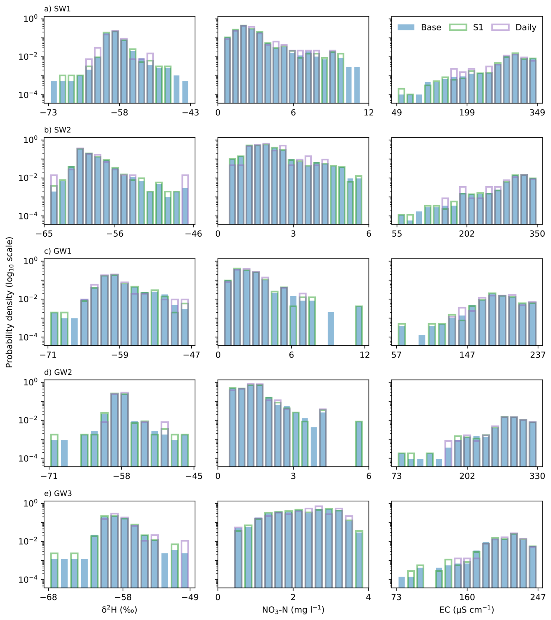
Figure 6 For each non-precipitation water source (a–e), probability density functions estimated via histograms for the deuterium (δ²H), nitrate (NO₃-N), and electrical conductivity (EC) data collected under the Baseline, S1 and Daily sampling scenarios. Note that probability density is on a log₁₀ scale to aid visualisation and x-axes are unique to each site and parameter.

Figure 6 shows the histograms for the Baseline and alternative sampling scenarios. For all measured parameters and water sources, the PDFs estimated for the Daily sampling scenario deviated most strongly from those of the Baseline. For NO₃-N, daily sampling captured fewer peaks in the data, resulting in a loss of probability density in the right tails of the PDFs. The exception was for GW3 (Fig. 6e), where NO₃-N concentrations in the Baseline were more evenly distributed and the effect of moving to daily sampling was less pronounced. The EC data displayed the opposite behaviour to NO₃-N, with daily sampling capturing fewer of the minimum values measured during precipitation events in the Baseline and reducing weight in the left tails of the PDFs. The effect of daily sampling on δ²H was more varied. Probability density was completely lost in the left tails of the PDFs for SW1 and GW1-3, likely due to under-sampling during the relatively rarer precipitation events with depleted δ²H measurements (Fig. 4b). Losses of probability density from the right tails were more fragmented, with daily sampling still able to capture some extreme values for SW2, GW1 and GW3. Probability density around the mean δ²H for each source was largely unchanged. In contrast to the Daily PDFs, those estimated for S1 largely reflected the characteristics of the PDFs estimated for the Baseline, including, for most sources and parameters, the length of the tails (although there could be some redistribution of probability density). Preservation of the tails was sometimes only possible due to the $\mathrm{24}/\mathrm{7}$ automated sampling by the WATER; for example, the outlying peaks in NO₃-N for GW1 and GW2 were both measured at night and would, therefore, never have been captured by usual daily sampling strategies.

Overall, the analysis of alternative sampling scenarios suggests that if deployed for a period of several months, the WATER could likely still capture the extremes of the measured parameters and certainly improve the characterisation of underlying data distributions relative to daily sampling, even if all 11 source inputs were in use. More caution would likely be required in the selection of which water sources to sample and at what frequency if individual event dynamics were of greater interest. However, sampling with the WATER in any configuration would likely provide greater insight than daily sampling alone.

5 Concluding remarks

This paper presented the Water Analysis Trailer for Environmental Research (WATER), the first example of an automated, mobile sampling platform capable of measuring the stable water isotope composition and water quality of multiple spatially distributed water sources at a high temporal frequency. Deployment of the WATER to the Schwingbach Environmental Observatory (SEO) provided proof-of-concept, demonstrating that the system could automatically acquire and measure samples from six water sources over a period of several months. Sub-sampling of the data to simulate sampling 11 water sources with the WATER suggested that the resultant reduced temporal sampling frequency would still capture much of the distribution of the measured parameters over longer time scales. Beyond the need for routine maintenance that would be necessary for any lab-in-the-field, the greatest challenge in operating the WATER for an extended period was ensuring the availability of sufficient power for continuous operation of the measurement devices. Therefore, when designing an experimental setup with the WATER, the potential trade-offs associated with prioritising a guaranteed power supply (i.e., mains power), mobility (i.e., self-sufficient power), or sustainability (i.e., solar over diesel power) should be carefully considered.

The type of data collection that is possible with the WATER was shown to have strong potential for improving process understanding in the SEO beyond previous studies based on coarser data. Significant scope exists for more formal hypothesis testing in relation to catchment functioning by integrating the data into data-driven and process-based models (Li et al., 2021), including those using isotopes to better constrain the flow paths responsible for connecting different solute sources in space and time (Wu et al., 2025). Furthermore, the flexibility offered by the design of the WATER also means that an even greater range of water sources and parameters could be analysed beyond those considered in the SEO. The mobile nature of the system also means that, over time, data can be gathered from multiple catchments using the same analytical setup to test the wider applicability of such hypotheses beyond a single catchment (Knapp et al., 2025). It may also be possible to rapidly deploy the WATER for analysis of extreme events (e.g., floods) or pollution incidents, subject to safe site access; this will be explored in future work. Overall, the WATER is likely to be a valuable tool for advancing our understanding of catchment hydrological and hydrochemical functioning.