Joint calibration of multi-scale hydrological data sets using probabilistic water balance data fusion: methodology and application to the irrigated Hindon River Basin, India

Hydrological data sets have vast potential for water resource management applications; however, they are subject to uncertainties. In this paper, we develop and apply a monthly probabilistic water balance data fusion approach for automatic bias correction and noise filtering of multi-scale hydrological data. The approach first calibrates the independent data sets by linking them through the water balance, resulting in hydrologically consistent estimates of precipitation (P), evaporation (E), storage (S), irrigation canal water imports (C), and river discharge (Q) that jointly close the basin-scale water balance. Next, the basin-scale results are downscaled to the pixel-scale, to generate calibrated ensembles of gridded Precipitation (P) and Evaporation (E) that reflect the basin-wide water balance closure constraints. An application to the irrigated Hindon River basin in India illustrates that the approach generates physically reasonable estimates of all basin-scale variables, with average standard errors decreasing in the following order: 21 mm month⁻¹ for storage, 10 mm month⁻¹ for evaporation, 7 mm month⁻¹ for precipitation, 4 mm month⁻¹ for irrigation canal water imports, and 2 mm month⁻¹ for river discharge. Results show that updating the original independent data with water balance constraint information reduces uncertainties by inducing cross-correlations between all independent variables linked through the water balance. In addition, the introduced approach yields (i) hydrologically consistent gridded P and E estimates that fuse information from prior (original) data across different land use elements and (ii) statistically consistent random errors that reflect the model's confidence about P and E estimates at each grid cell. The analysis also shows a long-term decreasing trend in groundwater, which is better captured by the more severe decline from GRACE JPL mascon than GRACE Spherical Harmonic data. This finding points towards the possible sustainability issues for irrigation in the basin and requires further validation using piezometer groundwater-level measurements. Future opportunities exist to further constrain the generated water balance variables and their associated errors within process-based models and with additional data.

1 Introduction

Under a changing climate and anthropogenic activities (Wada et al., 2010), it becomes urgent to accurately estimate the water balance components. Although distant from the Earth's surface, remote sensing (RS) satellites can uniquely provide information that translates into such estimates. For example, microwave and infrared techniques are used to estimate precipitation (Sun et al., 2018), evaporation can be computed using optical and thermal imagery (Zhang et al., 2016a), while changes in total water storage are obtained from the Gravity Recovery and Climate Experiment (GRACE) satellites (Wahr et al., 2004; Rodell et al., 2009). These advancements have emerged as powerful decision-support tools, pushing hydrology in new directions by providing valuable information on the spatial distribution of water availability, use, and consumption (Hessels et al., 2022; Sheffield et al., 2018; Karimi et al., 2013). Such information is often challenging to obtain through traditional in situ data collection. With the rapid increase in RS data availability, it is now theoretically possible to close the water balance. However, two challenges prevent this from being achieved, including the inconsistencies among various RS products for the same variable and the imbalances resulting from integrating the unique combinations of different water balance variables. These incoherences arise from the inherent data errors. Discrepancies in RS data, for example, come from different sources, such as errors in the retrieval algorithms (Maggioni et al., 2022), input data and parameters (Crosetto et al., 2001), or scale mismatch (Foken, 2008). While in situ data are known for their greatest reliability, they also come with their own errors. Uncertainties in river discharge, for example, could be related to flow conditions (Mcmillan et al., 2012), velocity sensors (e.g., calibration) (Horner et al., 2018), or estimation methods such as the rating curve (Kuczera, 1996). Benefiting from the complementary strengths of in situ and RS data and embracing their errors requires a three-pronged methodology. This methodology should maximize the prior information content of the data available from multiple RS sources for the same variable, quantify both systematic and random errors in each water balance term, and reduce these errors by exploiting all available information to generate calibrated estimates of spatially distributed water balance data. The following paragraphs review existing approaches in the literature used to handle these aspects.

Studies addressing the uncertainties in RS water balance data often rely on in situ data (treated as “ground-truth”) to evaluate and converge on the different data products. However, in situ data (e.g., evaporation) is sparsely measured, and even when these data exist, accessibility may be challenging. Under such conditions, alternative indirect approaches such as triple collocation (Tian and Peters-Lidard, 2010; Long et al., 2014; Massari et al., 2017; Yin and Park, 2021), uncertainty propagation (Hong et al., 2006; Cawse-Nicholson et al., 2020), and sensitivity analyses (Sobol, 2001) can be utilized. Other methods involve using the deviation from the ensemble mean, and the variability between the data sets as a proxy for uncertainty (Tian and Peters-Lidard, 2010; Sahoo et al., 2011; Munier et al., 2014; Zhang et al., 2018). Each of the previously summarized error estimation techniques has its inherent merits and shortcomings. In an attempt to capitalize on these strengths, Mourad et al. (2024) recently integrated limited in situ data and multiple error metrics, along with expert judgment, to quantify and partially reduce water balance data errors. However, the resulting water balance estimates require further conditioning on in situ data using additional constraining steps, which is a subject of the methodology section of the current study.

Several other studies went beyond quantifying uncertainties in RS data and sought to fully reduce them using the water balance as a constraint (Aires, 2014; Hobeichi et al., 2020; Luo et al., 2023; Munier et al., 2014; Pan et al., 2012; Pan and Wood, 2006; Rodell et al., 2015; Sahoo et al., 2011; Zhang et al., 2018, 2016b). The core idea of the existing closure methods is to either select a preferred single data set of each water balance variable based on prior knowledge about their quality, or merge multiple data for each water balance variable using fixed pre-quantified error estimates. This step is followed by a water balance correction method such as variational data assimilation (L'ecuyer and Stephens, 2002), constrained Kalman filter (Pan and Wood, 2006), or proportional redistribution (Abolafia-Rosenzweig et al., 2021). In this process, the values of the (un)merged water balance estimates are adjusted proportionally to their relative uncertainties or magnitudes, depending on the correction method used. Contrary to the previously summarized water balance closure approaches, which fixed data errors a priori, Schoups and Nasseri (2021) proposed improving data error estimation by treating them along with the water balance variables as unknown random variables. Instead of enforcing the closure sequentially, the authors demonstrate that the water balance variables can be calibrated simultaneously in a single probabilistic data fusion methodology. The underlying premise is that all variables are interconnected through the water balance. For instance, to calibrate precipitation data, the proposed approach uses statistical inference techniques to automatically fuse and adjust two information sources available on this variable, one coming from multiple estimates of precipitation RS data (original prior data), and the other sourced from other water balance data (predicted from the water balance). These techniques include an iterative smoother that involves multiple forward-backward passes over the timeseries. In the forward pass, the estimated precipitation carries information from previous and current months, while in the backward pass it holds information from the future months. A similar process happens when estimating the other water balance variables, yielding refined posterior estimates that combine information from all other months.

Further to the above literature, previous attempts have been made to extend the basin-wide water balance closure constraints to a finer scale of up to 0.25° pixel resolution (Barkhordari et al., 2025; Heberger et al., 2023; Pellet et al., 2019; Munier et al., 2014). Building on these previous efforts, our emphasis here is on generating detailed calibrated precipitation (0.05° resolution) and evaporation (250 m resolution) estimates that align with the basin-scale closure constraints. To that end, we intend to contribute to the literature by extending the existing basin-scale water balance data fusion method first introduced by Schoups and Nasseri (2021). The extended methodology presented here retains the original model's key advantages, namely: the ability to simultaneously calibrate the basin-wide water balance variables by exploiting data from the entire timeseries. An integral part of this new version is using the basin-wide posteriors to generate calibrated ensembles of spatially distributed precipitation and evaporation. This is achieved in a stepwise procedure, with the first step involving the formulation of ensemble-driven grid-scale error models, contrary to the models in Schoups and Nasseri (2021), which were formulated at the basin-scale and relied on an ensemble of two data sets. The second step is a constraint step carried out by the water balance data fusion at the basin scale, yielding basin-scale posteriors for all water balance variables, and a Kalman smoothing algorithm, yielding grid-scale posteriors for precipitation and evaporation. This approach ensures consistency across the two scales: when back-calculating the basin-scale estimates from the grid-scale posteriors via spatial averaging, we recover the inferred basin-scale posteriors from the water balance data fusion. Lastly, the new version of the methodology incorporates the following additional features: (i) accounting for surface water imports from irrigation canals, which might significantly affect the overall water budget in irrigated basins, and (ii) quantifying posterior cross-correlations between water balance variables, which is important for generating joint posterior samples. We apply the extended approach to an irrigated monsoon-influenced Hindon Basin, which suffers from unsustainable water use.

The remainder of this paper is structured as follows: Sect. 2 introduces the case study and describes the data sets used as input for the probabilistic water balance model presented in Sect. 3. Section 4 details how all unknowns in the water balance model are solved at the basin scale, yielding a closed water balance, and how these water balance constraints are transferred to the grid scale. The basin and grid-scale results are then presented in Sect. 5. The sensitivity of the water balance data fusion approach to the modeling decisions is then discussed in Sect. 6. Throughout the paper, we use the terms “priors” and “posteriors” to refer to the variables (i.e., water balance terms and error parameters) before and after calibration, respectively (i.e., before and after introducing the monthly water balance constraints).

2 Case Study: Hindon Basin in Northern India

The study focuses on the Hindon Basin in the northwestern Uttar Pradesh State of India (see Fig. 1). The Hindon basin covers a total area of about 4780 km² and drains to the Galeta outlet, where a river discharge station is located. The rainfed Hindon River originates from the Shivalik Hills at the foothills of the Himalayas. It flows towards the south on the flat and alluvial surfaces of the basin. The river eventually drains into the Yamuna River (near Noida, downstream of Delhi), which, in turn, joins the Ganga River before it reaches the Bay of Bengal. The basin features a large-scale supply-based irrigation system with two major irrigation canals: the Eastern Yamuna Canal (EYC) and the Upper Ganga Canal (UGC). These canals are fed by two external reservoirs located outside the basin, namely the Bhimgoda Barrage constructed on the Ganga River and Hathni Kund Headwork on the Yamuna River. The share of the external canal water imports in the water balance is significant for this heavily irrigated basin, representing about 30 %–40 % of the annual precipitation (Fig. A1). In addition to supplying surface irrigation water to the study area, the canals contribute to groundwater recharge through seepage, forming several groundwater mounds near their vicinity. Hence, the canals approximately coincide with groundwater divides, limiting lateral groundwater flow across the eastern and western boundaries of the Hindon basin (Umar et al., 2008).

The canal system is operated in two irrigation seasons: the Kharif and Rabi seasons. Kharif season extends from March to September, in which the main irrigated crops are sugarcane and rice, and the Rabi season spans from October to March of the following year, where the principal crops are wheat and mustard. The irrigated croplands represent more than 85 % of the basin, while only about 10 % of the basin's area is covered by non-croplands (Fig. A2). Irrigation water is diverted from the canals to supply the basin through off-takes that serve fixed command areas with crops rotated between Rabi and Kharif crops (Fig. 1).

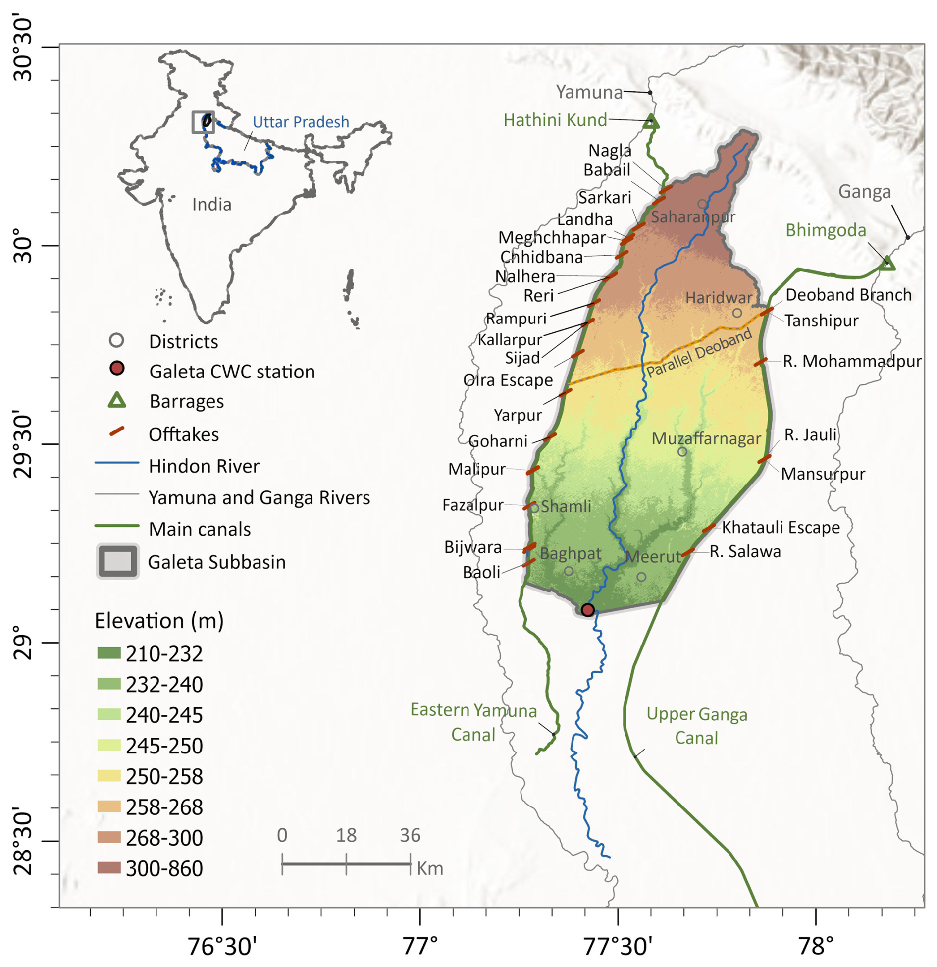
Figure 1 Location of the Hindon basin in the Uttar Pradesh state of India (inset map); with a detailed view of the basin featuring its boundaries, topographic profile, location of the Galeta outlet, where a river discharge station that belongs to the Central Water Commission (CWC) network of India is located. The main map shows the irrigation scheme with reservoirs and canal system. Topographic basemap sources: Esri, USGS, FAO, NPS, GIS user community, and others | Powered by Esri.

3 Probabilistic water balance model

Our goal is to estimate each term in the monthly water balance, written as:

$$\begin{array}{}\text{(1)}& S_t=S_{t-\mathrm{1}}+{\stackrel{\mathrm{‾}}{P}}_t-{\stackrel{\mathrm{‾}}{E}}_t-Q_t+C_t\end{array}$$

Equation (1) combines the different water balance terms together, where S_t−1 and S_t are the total water storage in the basin at the start and end of month t (including surface storage, soil moisture, and groundwater), ${\stackrel{\mathrm{‾}}{P}}_t$ and ${\stackrel{\mathrm{‾}}{E}}_t$ are the basin-average precipitation and evaporation (including transpiration), Q_t is the river discharge at the basin outlet for month t, and C_t is the total canal water import into the basin (sum of all intakes, see Fig. 1) for month t. The net lateral groundwater flows into or out of this basin are assumed to be negligible due to their small magnitude relative to the other water balance variables (Alam and Umar, 2013). All terms in Eq. (1) are expressed in units of mm of equivalent water depth. The following paragraphs describe the water balance data for the case study.

Each water balance component in Eq. (1) is independently derived, gathered, or measured either from satellite data, ground-based measurements, or both (Table 1). In the prior selection of the most reliable precipitation and evaporation ensembles (see Mourad et al., 2024), we followed other water balance closure studies that emphasize the use of earth observations over model outputs to minimize the effect of their related assumptions, except for the Multi-source Weighted-Ensemble Precipitation (MSWEP v2.8) product (Beck et al., 2019). MSWEP is an “optimal merging” of gauge observations, satellite observations, and reanalysis model output. Along with MSWEP, we use two other monthly gridded precipitation ensemble members: the Tropical Rainfall Measuring Mission (TRMM) (Huffman et al., 2007) and the NASA/JAXA Global Precipitation Measurement (GPM-IMERG) (Huffman et al., 2019). By combining precipitation radar, passive microwave, and infrared satellites with ground-based observations from the Global Precipitation Climatology Centre (GPCC), TRMM and GPM-IMERG provide a comprehensive precipitation estimate over a given area. Compared to single-band radar on TRMM, GPM dual-frequency precipitation radar provides a broader range of measurable precipitation rates and a better estimate of precipitation particle size (Hou et al., 2014). Spatially interpolated rain-gauge for the basin from Indian Meteorological Department (IMD) data set (Pai et al., 2014) is included in this analysis for comparison but not used in the model.

For gridded evaporation ensembles, we incorporate five members with diverse methodological approaches for estimating evaporation from remote sensing. One ET data set based on two-parallel Penman-Monteith (PM) models for both canopy and soil: the pyWaPOR-ET v2.6 (Bastiaanssen et al., 2012), two ET data sets that estimate ET from a single-source surface energy balance (SEB) model representing vegetation and soil in a combined energy balance, namely the Landsat Collection 2 Provisional Actual Evapotranspiration Science Product (Landsat-based SSEBop ET) (Senay, 2018; Senay et al., 2023) and the Surface Energy Balance Algorithm for Land (eeSEBAL product) (Bastiaanssen et al., 1993), in addition to a two-source SEB ALEXI-ET data set from the Atmosphere-Land Exchange Inverse model (Anderson et al., 2007, 2015). We also incorporate the CMRSET ET product based on the CSIRO MODIS Reflectance-based Scaling ET model (Guerschman et al., 2009) that uses vegetation indices and meteorological data for scaling the ET. All data sets are resampled to the same spatial resolution using bilinear interpolation. More details on the theoretical background and processing steps for the P and E data sets can be found in the companion paper (Mourad et al., 2024).

Table 1 Monthly Water Balance Data. The data type column distinguishes between Remote Sensing (RS) and ground-based Measurements (GBM).

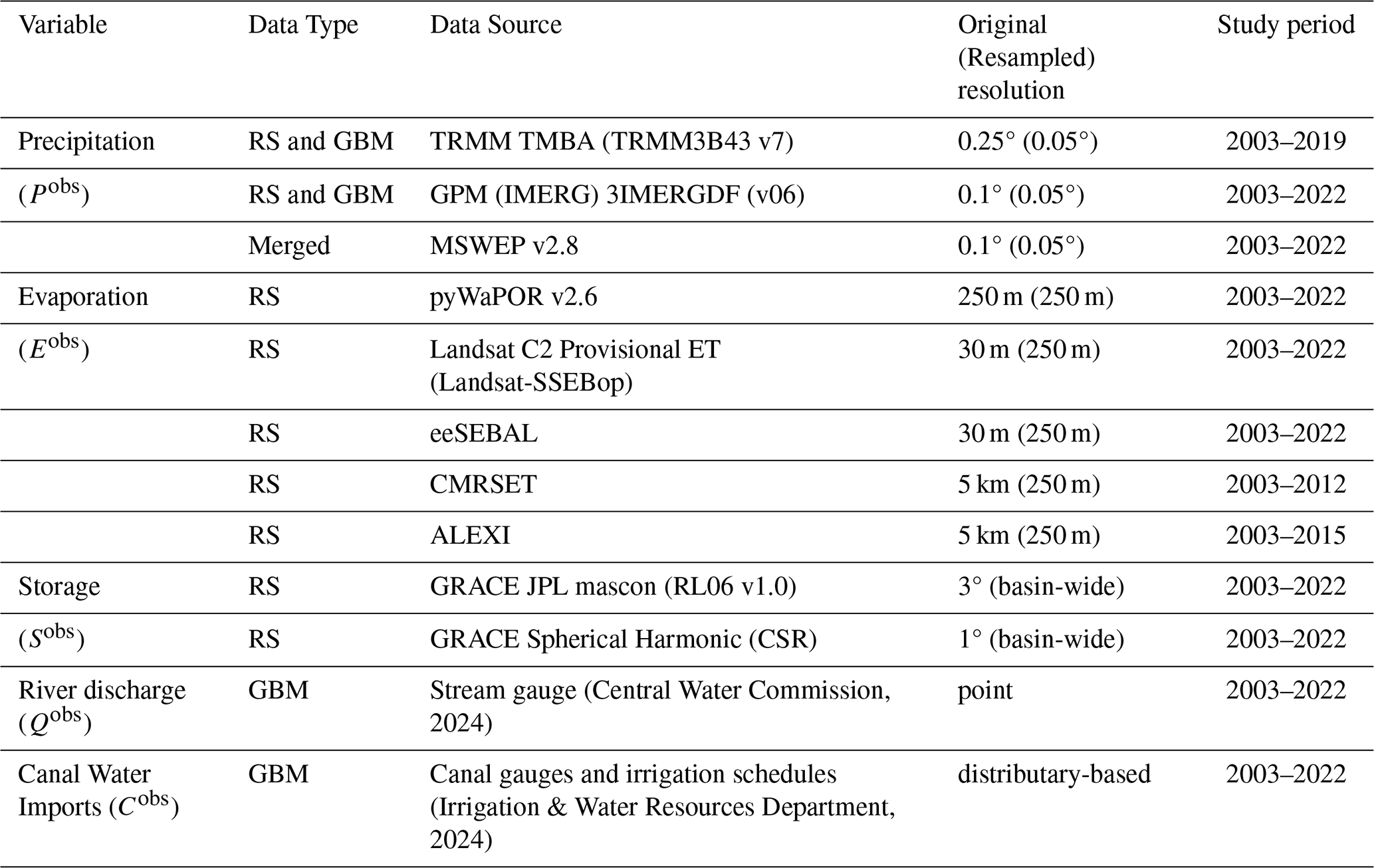
The total water storage variable data were obtained from the recent release of the monthly Jet Propulsion Laboratory (JPL-RL06) mascon solution. Each monthly total water storage estimate represents the surface mass anomaly relative to the baseline average over 2004–2009. This version relies on prior geophysical information to constrain the solution, eliminating the need for empirical de-striping filtering commonly used for post-processing traditional spherical harmonic gravity solutions. However, intrinsic to this product are biases, that is, leakage errors, and spatial smoothing that damps the “true” signal, especially in small-sized basins. A Coastline Resolution Improvement (CRI) filter has been applied in this version to reduce signal leakage errors across coastlines (Wiese et al., 2016). This data is also accompanied by scaling factors for optionally restoring the damped signal. However, these were not applied to the data used herein; instead, bias along with noise variance are modeled using all water balance data incorporated in this study (see Sect. 3.3). Another storage input data set is also included: GRACE Spherical Harmonic (CSR) solution (Sect. 6.1) (Swenson and Wahr, 2006; Landerer and Swenson, 2012).

The in situ data used in this analysis are obtained from governmental agencies, including the Central Water Commission (CWC) of India for streamflow data and the irrigation department of Uttar Pradesh for external canal water imports data. While river discharge data has no gaps, canal delivery data are constrained by their spatial and temporal coverage. The latter comes in two forms: irrigation schedules and actual flow measurements. We apply an extrapolation approach that combines both data sources to generate complete monthly estimates for all intakes (for more details on the adopted gap-filling technique, refer to Appendix  A2).

As can be seen in Table 1, the native resolution of the individual data sets and between the water balance variables varies widely, posing a challenge in their merging process. In principle, the probabilistic water balance data model can be performed at any spatial resolution; however, for this study design, we try to preserve the native information as much as possible by choosing to resample all precipitation data sets to a common resolution of 0.05° and all evaporation data sets to a common resolution of 250 m. An alternative design would be to resample all water balance variables to the same resolution (e.g., 250 m), but this might introduce artefacts, for example, when up-sampling from coarse to high resolution.

Despite the variety of the above-explored data sources, two barriers hinder their potential use in hydrological applications. One occurs when integrating the unique data combinations describing each water balance variable into the basin-scale water balance. In any particular month, we end up with significant errors, i.e., either too much or too little water, resulting in a non-zero net balance (Fig. B1 in Appendix B). This non-closure or imbalance problem highlights the incoherences between the water balance data sets and the inconsistencies in the individual data sets, caused by various data errors. Another well-known challenge is the inconsistencies between the various data products for the same variable. For example, for the studied basin, grid-scale inter-product uncertainty is moderate for P, while E exhibits significant spatial variability across the whole basin (Mourad et al., 2024). These challenges motivate the distinction between the “calibrated” value of each water balance variable that satisfies the water balance closure at the basin scale and represents the error-corrected estimate at the grid level, and the “observed” values, which deviate from these values. In the probabilistic form of the water balance, each term is assigned a probabilistic data error model to quantify systematic and random differences between observed and modelled water balance variables. Parameters in these data error models are treated as unknown random variables with predefined prior distributions. In this regard, the overall probabilistic water balance takes the form of a Bayesian hierarchical model with two levels of uncertainty: one related to the error parameters and another linked to the water balance variables (Schoups and Nasseri, 2021). Figure 2 gives an overview of our approach, and the following subsections describe the parametric probabilistic relations used for each water balance variable (P, E, Q, C, and S).

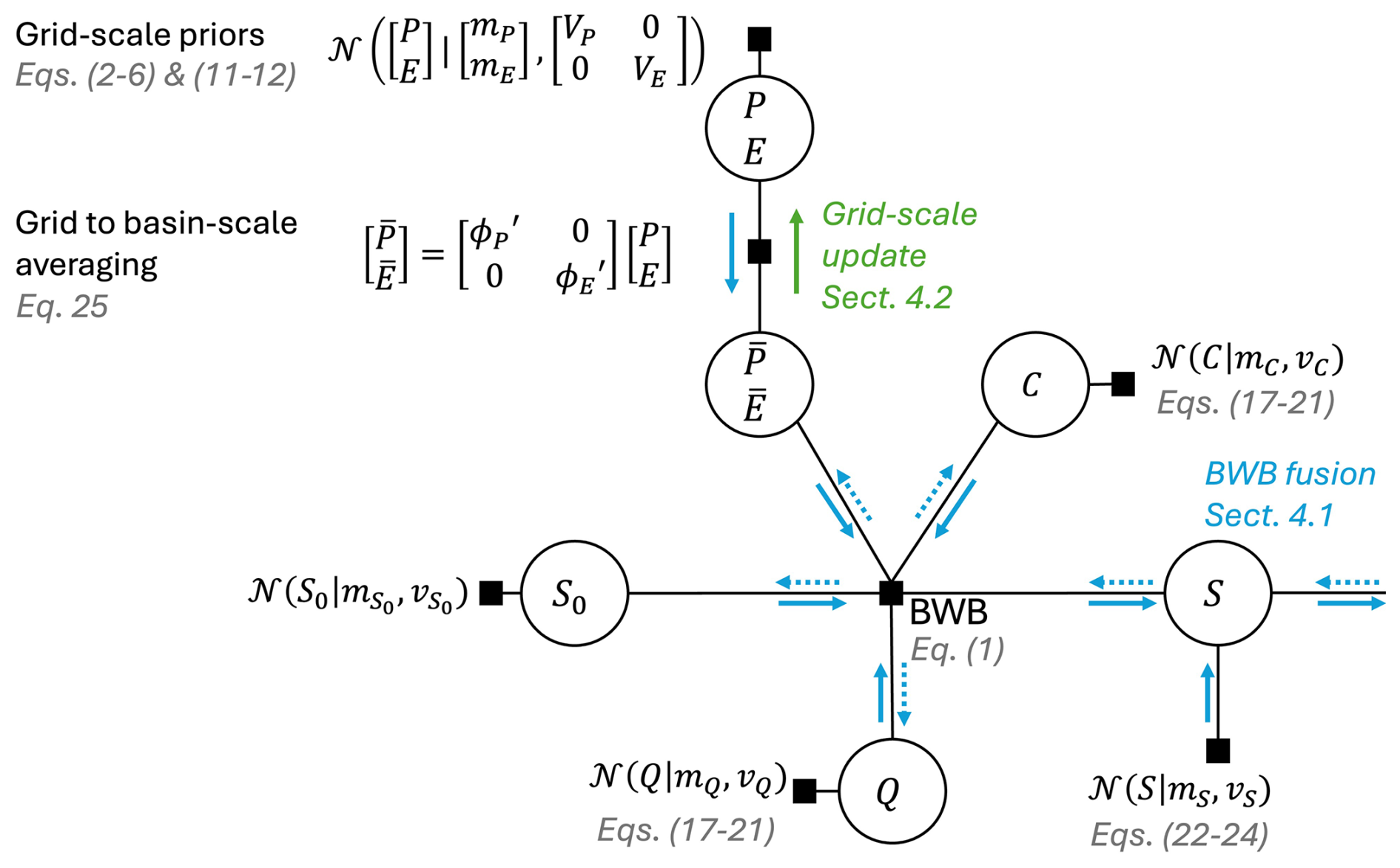
Figure 2 A factor graph showing random variables in circles and constraints between variables as squares for a single month. Three constraints are incorporated in the water balance data fusion method, including: a prior Gaussian distribution assigned to each water balance variable (squares attached to each variable), the basin-scale water balance (BWB) constraint that links all water balance variables together, and the spatial averaging constraint that links grid-scale precipitation (P) and evaporation (E) to basin-scale precipitation ($\stackrel{\mathrm{‾}}{P}$) and evaporation ($\stackrel{\mathrm{‾}}{E}$). Computation of posteriors of individual variables proceeds in two steps. The first step is basin-scale water balance data fusion (BWB fusion, see Sect. 4.1). This step involves multiple forward (blue arrows along the edges) and backward (dotted blue arrows) passes over the data using the entire timeseries to compute the posteriors of all water balance variables that jointly close the water balance (Schoups and Nasseri, 2021). The second step computes grid-scale posteriors for precipitation and evaporation from their basin-scale posteriors using a Kalman smoothing algorithm (green arrow, see Sect. 4.2).

3.1 Precipitation and Evaporation error models

Contrary to Schoups and Nasseri (2021), we define prior error models for P and E at the grid scale instead of at the basin scale, followed by spatial averaging to derive corresponding priors at the basin scale. The latter are then used with water balance data fusion for estimating basin-scale posteriors (Sect. 4.1). The resulting basin-scale posteriors are finally transferred back to the grid scale (Sect. 4.2).

The first step in setting up a prior error model for the gridded P and E variables is to probabilistically characterize them with prior distributions. For these two independent spatial processes, we can write their grid-scale joint prior distribution for each month t as:

$$\begin{array}{}\text{(2)}& \mathcal{N}\left(\left[\begin{array}{l}{\mathit{P}}_t\\ {\mathit{E}}_t\end{array}\right]\mathrm{|}\left[\begin{array}{l}{\mathit{m}}_{P_t}\\ {\mathit{m}}_{E_t}\end{array}\right],\left[\begin{array}{ll}{\mathbf{V}}_{P_t}& \mathrm{0}\\ \mathrm{0}& {\mathbf{V}}_{E_t}\end{array}\right]\right)\end{array}$$

where P_t and E_t are vectors containing unknown precipitation and evaporation values for all grid cells in the corresponding spatial field for each month t. The Gaussian distribution (Eq. 2) is specified with a mean vector and a block diagonal covariance matrix with zero cross-covariance to reflect that these two processes are assumed to be independent a priori. The mean vector consists of the prior means of P (${\mathit{m}}_{P_t}$) and E (${\mathit{m}}_{E_t}$), for all spatial locations within the corresponding spatial domain of each month t, while the autocovariance of each variable P (${\mathbf{V}}_{P_t}$) and E (${\mathbf{V}}_{E_t}$) is the block-diagonal element of the covariance matrix. The decomposed form of the joint distribution for each individual variable is described in the following subsections.

3.1.1 Precipitation

For each month t, we typically have multiple gridded precipitation products, with unknown bias and random errors. We use the spread across different precipitation products to define a grid-scale precipitation error model for the prior means ${\mathit{m}}_{P_t}$ (mean vector in Eq. 2) and the prior standard deviations ${\mathit{s}}_{P_t}$ (vector of the square root of all diagonal entries of the autocovariance matrix ${\mathbf{V}}_{P_t}$ in Eq. 2):

$$\begin{array}{}\text{(3)}& {\displaystyle }& {\displaystyle }{\mathit{m}}_{P_t}=(\mathrm{1}-w_P){\mathit{P}}_t^{\mathrm{obs},\min }+w_P{\mathit{P}}_t^{\mathrm{obs},\max }\text{(4)}& {\displaystyle }& {\displaystyle }{\mathit{s}}_{{\mathit{P}}_t}=r_P\mathrm{1}/\mathrm{4}\left({\mathit{P}}_t^{\mathrm{obs},\max }-{\mathit{P}}_t^{\mathrm{obs},\min }\right)\end{array}$$

Equation (3) models the systematic bias in grid-scale precipitation for each month t by describing the grid-scale precipitation prior means ${\mathit{m}}_{P_t}$ as a weighted average of the minimum (${\mathit{P}}_t^{\mathrm{obs},\min }$) and maximum (${\mathit{P}}_t^{\mathrm{obs},\max }$) precipitation for each grid cell. The weight or bias parameter w_P takes on an unknown value between 0 and 1, and is estimated from the data (see Sect. 4.1).

Random errors in grid-scale precipitation are modeled using Eq. (4). This model expresses the grid-scale prior standard deviations ${\mathit{s}}_{P_t}$ for each month t as a function of the difference between the maximum and minimum precipitation in each grid cell. A noise parameter (r_P), taking a value between 0 and 1, is used to scale the standard deviations. This parameter is also estimated from the data.

To account for the effect of spatial correlation of the random error component (Eq. 4), we write the precipitation prior covariance matrix ${\mathbf{V}}_{P_t}$ in terms of the grid-scale standard deviations and a grid-scale auto-correlation matrix:

$$\begin{array}{}\text{(5)}& {\mathbf{V}}_{P_t}={\mathbf{S}}_{P_t}{\mathbf{R}}_P{\mathbf{S}}_{P_t}\end{array}$$

where ${\mathbf{S}}_{P_t}$ is a diagonal matrix containing the grid-scale ${\mathit{s}}_{P_t}$ values for all locations of the spatial field (Eq. 4), and R_P is the correlation matrix that captures the spatial dependence structure. ${\mathbf{R}}_P\in {\mathbb{R}}^{n_P\times n_P}$, where n_P×n_P is the matrix dimension, and n_P equals 176, representing the total number of grid cell locations of the precipitation spatial domain. R_P is jointly estimated from all precipitation data using an isotropic parametric correlation function with the following form (Handcock and Stein, 1993):

$$\begin{array}{}\text{(6)}& C_{\mathcal{M}}\left(d\mathrm{|}{l}_{\mathrm{s}},v\right)={\displaystyle \frac{\mathrm{1}}{{\mathrm{2}}^{v-\mathrm{1}}\mathrm{\Gamma }\left(v\right)}}{\left({\displaystyle \frac{d}{l_{\mathrm{s}}}}\right)}^v{K}_v\left({\displaystyle \frac{d}{l_{\mathrm{s}}}}\right)\end{array}$$

where C_ℳ is the Matérn correlation function for variables separated by distance d. This correlation model is flexible and widely used, with two functions: gamma function Γ(.) and the modified Bessel function K_v(.) (Abramowitz and Stegun, 1968). C_ℳ also consists of two unknown nonnegative parameters, namely the spatial correlation length scale l_s and a spatial smoothness parameter ν. A value of ν approaching 0 indicates a rough spatial process, while the process is smoother when ν approaches infinity. Since the smoothness parameter is usually small in many applications (Chen et al., 2022), while it increases as the aggregation time increases (Sun et al., 2015), we choose a balanced value between a rough and smooth random field, i.e., ν, fixed at 1.5. On the other hand, the correlation length scale (l_s) defines an average length scale on which grid cells are correlated with each other. In principle, l_s ranges from 0 (the case of uncorrelated grid cells) and extends to a scale larger than the spatial domain length (the case of maximally correlated pixels). With no prior information on the l_s parameter, we fix it at 50 km ($\sim \mathrm{1}/\mathrm{2}$ the basin's length from North to South). The sensitivity of the results to the fixed l_s will be evaluated in Sect. 6.2.

Since water balance data fusion (Schoups and Nasseri, 2021) uses basin-scale error models, we derive these from the above-described grid-scale models by spatial averaging. Specifically, the basin-scale prior mean $m_{{\stackrel{\mathrm{‾}}{P}}_t}$ and variance $v_{{\stackrel{\mathrm{‾}}{P}}_t}$ in month t follow from Eqs. (3), (4), and (5):

$$\begin{array}{}\text{(7)}& {\displaystyle }{m}_{{\stackrel{\mathrm{‾}}{P}}_t}={\mathit{\varphi }}_P^{{}^{\prime }}{\mathit{m}}_{P_t}={\mathit{\varphi }}_P^{{}^{\prime }}\left[(\mathrm{1}-w_P){\mathit{P}}_t^{\mathrm{obs},\min }+w_P{\mathit{P}}_t^{\mathrm{obs},\max }\right]\end{array}$$

$$\begin{array}{}\text{(8)}& \begin{array}{rl}& v_{{\stackrel{\mathrm{‾}}{P}}_t}={\mathit{\varphi }}_P^{{}^{\prime }}{\mathit{V}}_{P_t}{\mathit{\varphi }}_P={\mathit{\varphi }}_P^{{}^{\prime }}{\mathbf{S}}_{P_t}{\mathbf{R}}_P{\mathbf{S}}_{P_t}{\mathit{\varphi }}_P\\ & ={\mathit{\varphi }}_P^{{}^{\prime }}\left(r_P{\mathbf{D}}_{P_t}\right){\mathbf{R}}_P\left(r_P{\mathbf{D}}_{P_t}\right){\mathit{\varphi }}_P\end{array}\end{array}$$

$$\begin{array}{}\text{(9)}& {\displaystyle }& {\displaystyle }\stackrel{\mathrm{‾}}{P_t}\sim \mathcal{N}\left(m_{{\stackrel{\mathrm{‾}}{P}}_t},v_{{\stackrel{\mathrm{‾}}{P}}_t}\right)\text{(10)}& {\displaystyle }& {\displaystyle }\stackrel{\mathrm{‾}}{P_t}\ge \mathrm{0}\end{array}$$

where ϕ_P is the spatial averaging operator used to derive basin-scale mean and variance from grid-scale means and variances (i.e., n_P×1 vector with each element equal to $\mathrm{1}/n_P$, where n_P is the number of spatial locations in the precipitation spatial field). ${\mathit{\varphi }}_P^{{}^{\prime }}$ is the transpose of ϕ_P. We also used ${\mathbf{S}}_{P_t}=r_P{\mathbf{D}}_{P_t}$, where D_P is a diagonal matrix containing the $\mathrm{1}/\mathrm{4}\left({\mathit{P}}_t^{\mathrm{obs},\max }-{\mathit{P}}_t^{\mathrm{obs},\min }\right)$ values (from Eq. 4) for all grid cells within the precipitation spatial field. All basin-averaged input quantities to Eqs. (7)–(8) are precomputed from the precipitation data sets, and the constant but unknown parameters w_P and r_P are estimated as part of the water balance data fusion (see Sect. 4.1).

Finally, the last two equations in the precipitation error model treat the basin-scale calibrated precipitation $\stackrel{\mathrm{‾}}{P_t}$ for each month t as a random draw from a truncated normal distribution. The truncation at zero ensures physical consistency (nonnegative precipitation).

3.1.2 Evaporation

As with precipitation, an evaporation error model with the following form is adopted:

$$\begin{array}{}\text{(11)}& {\displaystyle }& {\displaystyle }{\mathit{m}}_{E_t}=f_E\left[\right(\mathrm{1}-w_E){\mathit{E}}_t^{\mathrm{obs},\min }+w_E{\mathit{E}}_t^{\mathrm{obs},\max }]\text{(12)}& {\displaystyle }& {\displaystyle }{\mathit{s}}_{E_t}=r_E\mathrm{1}/\mathrm{4}\left({\mathit{E}}_t^{\mathrm{obs},\max }-{\mathit{E}}_t^{\mathrm{obs},\min }\right)\end{array}$$

The systematic bias in grid-scale evaporation is modeled with two spatial and time-invariant calibration parameters, namely: w_E and f_E. The parameter w_E is a bias parameter or weight that interpolates between the monthly grid-scale evaporation extrema $E_t^{\mathrm{obs},\min }$ and $E_t^{\mathrm{obs},\max }$. w_E takes on a value between 0 and 1, and is estimated from the data (see Sect. 4.1). An additional scaling factor (f_E) is incorporated to account for potential bias outside the observed grid-scale evaporation range, and is given a lognormal prior with mode at 1 (no bias) and a coefficient of variation CV of 50 %.

On the other hand, Eq. (12) quantifies the random errors in grid-scale evaporation, as the difference between the maximum and minimum evaporation in each grid cell. A noise parameter (r_E), taking a value between 0 and 1, is used to scale the random errors. All parameters are solved as part of the water balance data fusion (Sect. 4).

The basin-scale error models are derived from the grid-based models defined above, using the same spatial averaging process applied to precipitation (Eqs. 7–8). The averaging formulas are then obtained as follows:

$$\begin{array}{}\text{(13)}& {\displaystyle }{\displaystyle }{m}_{{\stackrel{\mathrm{‾}}{E}}_t}={\mathit{\varphi }}_E^{{}^{\prime }}{\mathit{m}}_{E_t}=f_E{\mathit{\varphi }}_E^{{}^{\prime }}\left[(\mathrm{1}-w_E){\mathit{E}}_t^{\mathrm{obs},\min }+w_E{\mathit{E}}_t^{\mathrm{obs},\max }\right]\end{array}$$

$$\begin{array}{}\text{(14)}& \begin{array}{rl}& v_{{\stackrel{\mathrm{‾}}{E}}_t}={\mathit{\varphi }}_E^{{}^{\prime }}{\mathbf{V}}_{E_t}{\mathit{\varphi }}_E={\mathit{\varphi }}_E^{{}^{\prime }}{\mathbf{S}}_{E_t}{\mathbf{R}}_E{\mathbf{S}}_{E_t}{\mathit{\varphi }}_E\\ & ={\mathit{\varphi }}_E^{{}^{\prime }}\left(r_E{\mathbf{D}}_{E_t}\right){\mathbf{R}}_E\left(r_E{\mathbf{D}}_{E_t}\right){\mathit{\varphi }}_E\end{array}\end{array}$$

$$\begin{array}{}\text{(15)}& {\displaystyle }& {\displaystyle }\stackrel{\mathrm{‾}}{E_t}\sim \mathcal{N}(m_{{\stackrel{\mathrm{‾}}{E}}_t},v_{{\stackrel{\mathrm{‾}}{E}}_t})\text{(16)}& {\displaystyle }& {\displaystyle }\stackrel{\mathrm{‾}}{E_t}\ge \mathrm{0}\end{array}$$

where D_E is a diagonal matrix whose diagonal entries contain the $\mathrm{1}/\mathrm{4}\left({\mathit{E}}_t^{\mathrm{obs},\max }-{\mathit{E}}_t^{\mathrm{obs},\min }\right)$ values for all grid cells within the evaporation spatial domain. All inputs of Eqs. (13)–(14) are precomputed from the evaporation data sets. ϕ_E is the spatial averaging operator, and the R_E term stands for the correlation matrix, which captures the spatial dependencies between the evaporation grid cells ${\mathit{R}}_E\in {\mathbb{R}}^{n_E\times n_E}$, where n_E×n_E is the matrix dimension, and n_E equals 71059, representing the total number of grid cell locations of the evaporation spatial domain. For the large-sized evaporation data sets considered here, we parameterize the evaporation correlation matrix using a Matérn Gaussian Process kernel (Hensman et al., 2015) with fixed parameters l_s at 50 km and ν at 1.5.

Similar to precipitation, the basin-scale calibrated evaporation $\stackrel{\mathrm{‾}}{E_t}$ for month t is treated as a random draw from a truncated normal distribution Eqs. (15)–(16). The truncation at zero ensures physical consistency (nonnegative evaporation).

3.2 River discharge and canal water import error models

We assume that data on river discharge (Q^obs) and canal water imports (C^obs) are both unbiased with proportional random errors (Eq. 18). Both variables are modelled as truncated Gaussian variables (non-negative), with mean $m_{x_t}$, standard deviation $s_{x_t}$, and variance $v_{x_t}$ in month t given by:

$$\begin{array}{}\text{(17)}& {\displaystyle }& {\displaystyle }{m}_{x_t}=x_t^{\mathrm{obs}}\text{(18)}& {\displaystyle }& {\displaystyle }{s}_{x_t}=a_x{x}_t^{\mathrm{obs}}\text{(19)}& {\displaystyle }& {\displaystyle }{v}_{x_t}=s_{x_t}^{\mathrm{2}}\text{(20)}& {\displaystyle }& {\displaystyle }{x}_t\sim \mathcal{N}(m_{x_t},v_{x_t})\text{(21)}& {\displaystyle }& {\displaystyle }{x}_t\ge \mathrm{0}\end{array}$$

where $x_t^{\mathrm{obs}}$ represents the observed value for each month $t(Q_t^{\mathrm{obs}}$ for discharge and $C_t^{\mathrm{obs}}$ for canal water imports). $s_{x_t}$ quantifies the random errors in Q^obs or C^obs, and is assumed proportional to the observed value, with a proportionality constant (or relative error) a_x. We assume a 10 % relative error for monthly river discharge, i.e., a_Q=0.1, and a 25 % relative error for canal water imports, i.e., a_C=0.25.

3.3 Water Storage Error Model

The water storage error model relates the storage observations from the GRACE satellite ($S_t^{\mathrm{obs}}$) to the modeled storage (S_t). Due to the coarse resolution of GRACE data, the monthly basin-scale total water storage derived from these observations can be polluted by the water storage dynamics occurring outside the basin, that is, “leakage”. To account for the temporal and spatial mismatch between GRACE basin-scale water storage and the modeled storage caused by leakage errors, we employ the following noisy sine wave error model (Schoups and Nasseri, 2021):

$$\begin{array}{}\text{(22)}& {\displaystyle }& {\displaystyle }{m}_{S_t}=S_t+A\sin \left(\mathit{\omega }\left({\displaystyle \frac{t}{\mathrm{12}}}-\mathit{\delta }\right)\right)\text{(23)}& {\displaystyle }& {\displaystyle }{v}_{S_t}={\mathit{\sigma }}_S^{\mathrm{2}}\text{(24)}& {\displaystyle }& {\displaystyle }{S}_t^{\mathrm{obs}}\sim \mathcal{N}(m_{S_t},v_{S_t})\end{array}$$

The first equation models the systematic errors associated with GRACE observations. It captures cyclic patterns and seasonality in the data within the basin via time-invariant error parameters. These parameters describe the magnitude and the timing of the seasonal error: the amplitude A (mm) and phase δ (years), respectively.

The magnitude of random errors is modeled as an unknown time-invariant parameter (σ_S), which reflects errors that can arise from (a) any limitations caused by the sine wave models in capturing the calibrated water storage dynamics within the basin and (b) noise in GRACE solutions. In the above equations, ω is fixed at 2π radians per year, yielding a one-year sine wave and thus capturing the annual seasonal cycle. Other parameters are assigned vague prior distributions, where A follows a lognormal prior with mode at 30 mm and a CV of 200 %, σ_S a lognormal prior with mode equal to 10 mm and a CV of 200 %, and δ follows a flat logit-normal prior between 0 and 1 year with a location parameter μ=0 and scale parameter σ=1.4.

While the above prior error model relies on a single storage data set, we assess a posteriori (Sect. 6.1) the sensitivity of the P and E posterior distributions to the use of different storage inputs, including Mascon (JPL) and Spherical Harmonic (CSR) GRACE solutions, which for the basin studied here, exhibit different long-term trends.

4 Inference methods

The following subsections detail the two-step statistical inference framework used to solve the basin-scale probabilistic water balance model (Sect. 4.1) and then propagate the resulting basin-wide constraints to the grid level (Sect. 4.2).

4.1 Basin-scale

Following the description of the prior probabilistic relations (Sect. 3), the posteriors of water balance variables and error parameters are computed using a basin-scale inference technique. This technique consists of a double-loop method that combines two algorithms: a single-chain differential evolution variant of Markov Chain Monte Carlo (DE-MCMC) for computing the unknown parameters and Expectation Propagation (EP) for solving the unknown water balance variables. A brief overview of these algorithms is described in Appendix B, while a detailed explanation can be found in the original paper (Schoups and Nasseri, 2021). The computed posteriors provide hydrologically consistent water balance variables that jointly close the water balance. In the water balance data fusion process, the independent prior data (Sect. 3) are updated with the monthly water balance constraints. These constraints link all independent variables through the water balance, thereby inducing cross-correlation between them. For example, the term S in the water balance constraint (dropping the time index t for simplicity: $S=S_{\mathrm{0}}+\stackrel{\mathrm{‾}}{P}-\stackrel{\mathrm{‾}}{E}-Q+C$) linearly links all other terms. To maintain the water balance closure, the terms with opposite signs must covary together, and vice versa. In this paper, an additional post-processing step is applied to represent this interdependence structure between the water balance variables, i.e., compute their covariances. For a vector of posterior variables x (including the initial storage state S₀ or S_t−1, $\stackrel{\mathrm{‾}}{P}$, $\stackrel{\mathrm{‾}}{E}$, Q, and C), a joint distribution can be written for each month t as: $p\left(x_t\right)\sim \mathcal{N}\left({\mathit{m}}_{x,t}^{\ast },{\mathbf{V}}_t^{\ast }\right)$ with a mean vector (${\mathit{m}}_{x,t}^{\ast }$) holding the marginal posterior means of each variable (Eq. B2) and a 5×5 covariance matrix ${\mathbf{V}}_t^{\ast }$ that encodes the relation between these variables. The diagonal element of this matrix contains each variable's marginal posterior variance, while the unknown covariances between each variable pair are the off-diagonal entries. To quantify these covariances, a message-passing algorithm that combines the water balance constraint and the probabilistic constraints in the form of marginal Gaussian distributions is applied (see Sect. B2 in Appendix B).

4.2 Grid-scale

Having computed the joint basin-scale $\stackrel{\mathrm{‾}}{P}$ and $\stackrel{\mathrm{‾}}{E}$ posteriors (Sect. 4.1), the goal is to translate these posteriors back to the grid-scale. When spatially averaged, the generated grid-scale posteriors (P and E) should recover the basin-scale posteriors. Such a relation between the two scales can be established for each month t as follows (Eq. 25):

$$\begin{array}{}\text{(25)}& \left[\begin{array}{l}{\stackrel{\mathrm{‾}}{P}}_t\\ {\stackrel{\mathrm{‾}}{E}}_t\end{array}\right]=\mathbf{A}\left[\begin{array}{l}{\mathit{P}}_t\\ {\mathit{E}}_t\end{array}\right]\end{array}$$

where $\mathbf{A}=\left[\begin{array}{ll}{\mathit{\varphi }}_P^{\prime }& \mathrm{0}\\ \mathrm{0}& {\mathit{\varphi }}_E^{\prime }\end{array}\right]$ represents the spatial averaging operator mapping the grid-scale to the basin-scale P and E variables, ϕ_P and ϕ_E are defined earlier in Eqs. (7, 13).

For the above relation to hold (Eq. 25), we implement a Kalman smoothing algorithm. A key aspect of this algorithm is that it ties together all sources of information on P and E variables, detailed in previous sections, including: the basin and grid-scale joint priors (Sect. 3), along with basin-scale joint posteriors (Sect. 4.1), to generate their corresponding spatially distributed joint posteriors. Distinctly, the grid-scale prior moments (Eq. 2) are updated to reflect the difference between the basin-scale joint posterior and prior moments via the Kalman gain. In what follows, we start by describing the basin-scale joint prior and posterior distributions and then show how the grid-scale joint distributions are computed.

Before constraining the basin-scale spatially averaged $\stackrel{\mathrm{‾}}{P_t}$ and ${\stackrel{\mathrm{‾}}{E}}_t$ priors, their joint distribution for each month tcan be written with zero-cross covariances to reflect the independent structure between both variables:

$$\begin{array}{}\text{(26)}& \mathcal{N}\left(\left[\begin{array}{l}\stackrel{\mathrm{‾}}{P_t}\\ {\stackrel{\mathrm{‾}}{E}}_t\end{array}\right]\mathrm{|}\left[\begin{array}{l}{m}_{{\stackrel{\mathrm{‾}}{P}}_t}\\ m_{{\stackrel{\mathrm{‾}}{E}}_t}\end{array}\right],\left[\begin{array}{ll}{v}_{{\stackrel{\mathrm{‾}}{P}}_t}& \mathrm{0}\\ \mathrm{0}& v_{{\stackrel{\mathrm{‾}}{E}}_t}\end{array}\right]\right)\end{array}$$

where $m_{{\stackrel{\mathrm{‾}}{P}}_t}$ and $m_{{\stackrel{\mathrm{‾}}{E}}_t}$ are prior means, $v_{{\stackrel{\mathrm{‾}}{P}}_t}$ and $v_{{\stackrel{\mathrm{‾}}{E}}_t}$ are prior variances of $\stackrel{\mathrm{‾}}{P_t}$ and ${\stackrel{\mathrm{‾}}{E}}_t$, respectively.

Once the water balance constraint is imposed within the basin-scale data fusion: $\stackrel{\mathrm{‾}}{P}-\stackrel{\mathrm{‾}}{E}-Q+C+S_{\mathrm{0}}-S=\mathrm{0}$ (omitting t for simplicity), positive correlations between $\stackrel{\mathrm{‾}}{P}$ and $\stackrel{\mathrm{‾}}{E}$ posteriors emerge. This occurs because the water balance acts as a constraint on the priors (independent $\stackrel{\mathrm{‾}}{P}$ and $\stackrel{\mathrm{‾}}{E})$ linearly linking them in their posteriors (correlated $\stackrel{\mathrm{‾}}{P}$ and $\stackrel{\mathrm{‾}}{E}$). To maintain this linear constraint, that is, $\stackrel{\mathrm{‾}}{P}-\stackrel{\mathrm{‾}}{E}$ remains equal to $Q-C-S_{\mathrm{0}}+S$, an adjustment that increases $\stackrel{\mathrm{‾}}{P}$ should be balanced by an adjustment that increases $\stackrel{\mathrm{‾}}{E}$ , and vice versa. This yields a basin-scale joint posterior distribution on the posterior variables $\stackrel{\mathrm{‾}}{P_t}$ and ${\stackrel{\mathrm{‾}}{E}}_t$, with induced correlations, that is, non-zero cross covariances:

$$\begin{array}{}\text{(27)}& \mathcal{N}\left(\left[\begin{array}{l}\stackrel{\mathrm{‾}}{P_t}\\ {\stackrel{\mathrm{‾}}{E}}_t\end{array}\right]\mathrm{|}\left[\begin{array}{l}{m}_{{\stackrel{\mathrm{‾}}{P}}_t}^{\ast }\\ m_{{\stackrel{\mathrm{‾}}{E}}_t}^{\ast }\end{array}\right],\left[\begin{array}{ll}{v}_{{\stackrel{\mathrm{‾}}{P}}_t}^{\ast }& v_{{\stackrel{\mathrm{‾}}{PE}}_t}^{\ast }\\ v_{{\stackrel{\mathrm{‾}}{PE}}_t}^{\ast }& v_{{\stackrel{\mathrm{‾}}{E}}_t}^{\ast }\end{array}\right]\right)\end{array}$$

where $m_{{\stackrel{\mathrm{‾}}{P}}_t}^{\ast }$ and $m_{{\stackrel{\mathrm{‾}}{E}}_t}^{\ast }$ are the marginal posterior means, $v_{{\stackrel{\mathrm{‾}}{P}}_t}^{\ast }$ and $m_{{\stackrel{\mathrm{‾}}{E}}_t}^{\ast }$ are the marginal posterior variances of $\stackrel{\mathrm{‾}}{P_t}$ and ${\stackrel{\mathrm{‾}}{E}}_t$, respectively, and $v_{{\stackrel{\mathrm{‾}}{PE}}_t}^{\ast }$ is the posterior cross-covariance between $\stackrel{\mathrm{‾}}{P_t}$ and ${\stackrel{\mathrm{‾}}{E}}_t$.

Kalman smoothing can then be used to calculate the joint posterior moments Eqs. (28)–(29) at the grid-scale from the above basin-scale prior moments Eqs. (26)–(27) and grid-scale prior moments (Eq. 2). These posterior moments are thus rendered as a weighted combination of grid and basin-scale moments:

$$\begin{array}{}\text{(28)}& \left[\begin{array}{l}{\mathit{m}}_{P_t}^{\ast }\\ {\mathit{m}}_{E_t}^{\ast }\end{array}\right]=\left[\begin{array}{c}{\mathit{m}}_{P_t}\\ {\mathit{m}}_{E_t}\end{array}\right]+\mathbf{K}\left(\left[\begin{array}{l}{m}_{{\stackrel{\mathrm{‾}}{P}}_t}^{\ast }\\ m_{{\stackrel{\mathrm{‾}}{E}}_t}^{\ast }\end{array}\right]-\left[\begin{array}{c}{m}_{{\stackrel{\mathrm{‾}}{P}}_t}\\ m_{{\stackrel{\mathrm{‾}}{E}}_t}\end{array}\right]\right)\end{array}$$

$$\begin{array}{}\text{(29)}& \begin{array}{rl}& \left[\begin{array}{ll}{\mathbf{V}}_{P_t}^{\ast }& {\mathbf{V}}_{P{E}_t}^{\ast }\\ {\mathbf{V}}_{P{E}_t}^{{\ast }^{{}^{\prime }}}& {\mathbf{V}}_{E_t}^{\ast }\end{array}\right]=\left[\begin{array}{ll}{\mathbf{V}}_{P_t}& \mathrm{0}\\ \mathrm{0}& {\mathbf{V}}_{E_t}\end{array}\right]\\ & +\mathbf{K}\left(\left[\begin{array}{ll}{v}_{{\stackrel{\mathrm{‾}}{P}}_t}^{\ast }& v_{{\stackrel{\mathrm{‾}}{PE}}_t}^{\ast }\\ v_{{\stackrel{\mathrm{‾}}{PE}}_t}^{\ast }& v_{{\stackrel{\mathrm{‾}}{E}}_t}^{\ast }\end{array}\right]-\left[\begin{array}{cc}{v}_{{\stackrel{\mathrm{‾}}{P}}_t}& \mathrm{0}\\ \mathrm{0}& v_{{\stackrel{\mathrm{‾}}{E}}_t}\end{array}\right]\right){\mathbf{K}}^{{}^{\prime }}\end{array}\end{array}$$

where ${\mathit{m}}_{P_t}^{\ast }$ and ${\mathit{m}}_{E_t}^{\ast }$ are the grid-scale means, while ${\mathbf{V}}_{P_t}^{\ast }$ and ${\mathbf{V}}_{E_t}^{\ast }$ are autocovariances of P_t and E_t posteriors, respectively. ${\mathbf{V}}_{P{E}_t}^{\ast }$ and ${\mathbf{V}}_{P{E}_t}^{{\ast }^{{}^{\prime }}}$ stand for the posterior cross-covariance between both variables and its transpose, respectively.

A noteworthy feature of the Kalman smoothing gain (K) in the above equations is that it acts as a weighting matrix propagating basin-scale information to each individual P and E grid cell. It is computed using the following equation composed of three components:

$$\begin{array}{}\text{(30)}& \mathbf{K}=\left[\begin{array}{ll}{\mathbf{V}}_{P_t}& \mathrm{0}\\ \mathrm{0}& {\mathbf{V}}_{E_t}\end{array}\right]{\mathbf{A}}^{{}^{\prime }}{\left[\begin{array}{ll}{v}_{{\stackrel{\mathrm{‾}}{P}}_t}& \mathrm{0}\\ \mathrm{0}& v_{{\stackrel{\mathrm{‾}}{E}}_t}\end{array}\right]}^{-\mathrm{1}}\end{array}$$

The first component depicts the block diagonal covariance matrix of the grid-scale P_t and E_t priors, the second is the transpose of the spatial averaging operator A, whereas the inverse of the diagonal matrix consisting of the basin-wide variances of $\stackrel{\mathrm{‾}}{P_t}$ and ${\stackrel{\mathrm{‾}}{E}}_t$ priors is the third component.

5 Results

Here, we present the results of the two-step inference framework described in Sect. 4, starting with the basin-scale posteriors of all water balance variables (Sect. 5.1) and followed by the grid-scale posteriors of P and E (Sect. 5.2). These represent the baseline results that are based on specific choices of GRACE data (i.e., JPL mascon data) and spatial correlation lengths. The sensitivity of the results to these choices will be addressed in Sect. 6.

5.1 Basin-scale posteriors

Basin-scale posteriors for P (precipitation), E (evaporation), and C (canal water imports) are shown in Fig. 3 and discussed first. The data shows significant prior uncertainty with a wide range of precipitation and evaporation estimates. This is especially evident in the monsoon (June to September) for precipitation and across the whole seasonal cycle for evaporation (Fig. 3). Along with the prior observations, Fig. 3 also depicts the basin-scale posteriors for each water balance term, while Fig. 4 shows the corresponding error parameter posteriors. The results for Q are not included in Fig. 3 since the posterior for Q closely follows the river discharge data, and this data is tied to a non-disclosure agreement with the CWC of India.

The results in Fig. 3 show that the precipitation posterior mean lies between the ${\stackrel{\mathrm{‾}}{P}}_t^{\mathrm{obs},\min }$ and ${\stackrel{\mathrm{‾}}{P}}_t^{\mathrm{obs},\max }$ data bounds. This balanced position within the precipitation space is also translated into the inferred parameter w_P, with a posterior distribution around values of ∼0.5 (Fig. 4). The noise parameter r_P has a posterior distribution around 1, suggesting a minimal reduction in the prior uncertainty range for precipitation. An independent evaluation of these posterior estimates can be done by comparing them to the Indian Meteorological Department (IMD) data set (Pai et al., 2014), which is routinely used to evaluate precipitation products in India. Despite being treated as the “ground truth” in literature, the rain-gauge interpolated IMD product is not error-free, and therefore, a perfect match between the IMD data and the generated posterior mean is not anticipated. Figure C1 in Appendix C compares the seasonal and annual timeseries of the IMD to the posterior precipitation mean. Unlike the precipitation posterior mean, which tends to sit between observed data bounds, the IMD data set closely follows the baseline precipitation estimate (TRMM). The larger posterior estimates for P found here align with a recent study (Goteti and Famiglietti, 2024) that found systematic underestimation of precipitation by the IMD data product. Moving to evaporation, the computed posteriors in Fig. 3 only slightly differ from the priors, with posterior values of noise parameter r_E centered at ∼0.95 (Fig. 3), implying that the modeled random error in this variable is as large as one-fourth of the absolute difference between ${\stackrel{\mathrm{‾}}{E}}_t^{\mathrm{obs},\min }$ and ${\stackrel{\mathrm{‾}}{E}}_t^{\mathrm{obs},\max }$. This posterior uncertainty, however, reduces with a tighter data range corresponding to prior ensembles generated from only three data sets: eeSEBAL, pyWaPOR, and Landsat-SSEBop (specifically, from 2015 onwards). As for the estimated evaporation, it takes more or less a balanced weight between ${\stackrel{\mathrm{‾}}{E}}_t^{\mathrm{obs},\min }$ and ${\stackrel{\mathrm{‾}}{E}}_t^{\mathrm{obs},\max }$, with an estimated w_E posterior of ∼0.48 and a scaling parameter f_E around 1 (no additional bias). While no direct evaporation measurements are available, the posterior estimates can be evaluated by comparing them with reference evapotranspiration and expected seasonal dynamics based on known cropping and irrigation practices. For example, the evaporation is expected to be lower than ${\stackrel{\mathrm{‾}}{ET}}_{\mathrm{0}}$ but equal to or higher than the ${\stackrel{\mathrm{‾}}{ET}}_{\mathrm{0}}$ for only a short period, either in June–July or August–October, when the (dominant) sugarcane crop coefficient (Kc) exceeds 1. In Fig. 3, the inferred posterior evaporation (green band) aligns with this expectation where it is consistently below ${\stackrel{\mathrm{‾}}{ET}}_{\mathrm{0}}$, but is also around ${\stackrel{\mathrm{‾}}{ET}}_{\mathrm{0}}$ for the previously mentioned period (e.g., in 2006, 2012, 2019, and 2022). Besides sugarcane, rice is the second most important crop, commonly transplanted at the end of April or mid-May (Joseph and Ghosh, 2023). For this shallow-rooted crop, more frequent irrigation is required during its early stages (the first 30 d), coinciding with the period when the canal water supplies form a peak (at the onset of the monsoon) (Fig. C3 in Appendix C). The evaporation timeseries of rice is, thus, expected to form a peak, most likely in June, when its Kc value is higher than 1. Considering these two elements, the evaporation is expected to peak in June, as captured by the posterior evaporation mean (Fig. C2 in Appendix C).

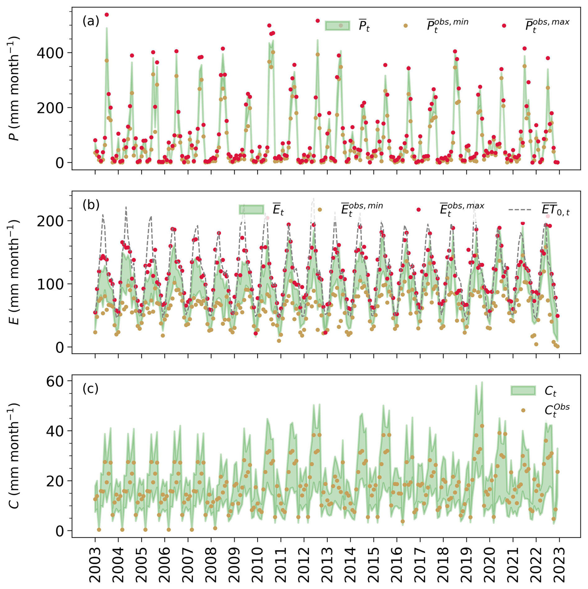
Figure 3 Monthly water balance posteriors (90 % credible intervals in green) for: (a) P (precipitation), (b) E (actual evapotranspiration), and (c) C (canal water imports), and their corresponding observations (dots). Reference evapotranspiration computed here using ERA5 meteorological input variables is shown as (ET₀). The overbars of the labels in P and E plots indicate that these values are obtained through spatial averaging of the gridded data sets for each month t. Each year's label indicates the start of the year (January).

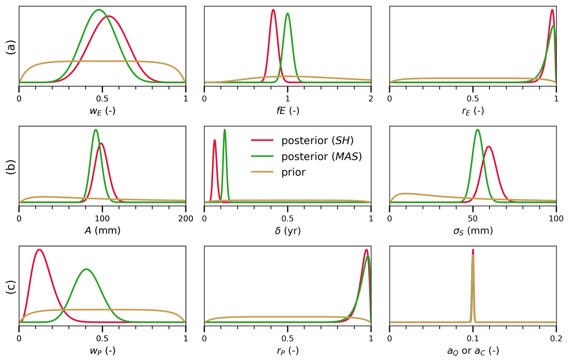
Figure 4 Prior and posterior distributions of error parameters for: (a) evaporation, (b) storage, (c) precipitation, canal water import, and river discharge when using different GRACE storage data sets: CSR Spherical Harmonic (SH) and JPL Mascon (MAS) solutions.

The third row of Fig. 3 compares the prior and posterior estimates of the canal water imports (C). The prior estimates represented here are extrapolated from scarce data. Nevertheless, the extrapolation approach mostly relied on ground-based measurements whenever available. For periods with missing data, these were filled with the design discharge capacity multiplied by the operation time or the data average of years with similar conditions, depending on data availability per distributary. For this purpose, independent information from the Palmer Drought Severity Index (PDSI) index of the Terra Climate data set (Abatzoglou et al., 2018) is used as a proxy to classify the years between wet and dry, allowing for annual variations in the canal water supply. For example, in dry years, such as 2008, and 2016 to 2018, the surface water supplies are smaller in magnitude compared to all other years. Note also the increase in the water supplies from 2009 onwards, which aligns with the construction of the Deoband Parallel Canal that connects the Upper Ganga Canal (UGC) to the Eastern Yamuna Canal (EYC) (Fig. 1). Using other approaches to generate and extrapolate the prior canal water estimates does not significantly affect the posteriors of the other terms, as explored in Sect. 6.3. The posterior results, on the other hand, reflect the wide prior uncertainty (relative error of 25 %) we place around this extrapolated data. Generally, the posterior estimates follow both their priors and the seasonality of the precipitation term. Specifically, the supplies peak at the onset of the monsoon (June) due to increased water availability from precipitation, while smaller peaks are formed during the dry season (December and April) when water stored in the reservoirs is diverted for irrigation. As canal supplies are mainly driven by precipitation, it is reasonable to conclude that the canal water imports are smaller in magnitude compared to precipitation during the rainy months (July–September), representing about 5 % to 15 % of the monthly precipitation. It follows that the fixed prior uncertainty on this term is a justifiable approximation that does not strongly affect the other water balance estimates.

Finally, we note the interplay between all variables: water balance (P, E, C, and Q), weather, and crop variables. Despite relying on external water supplies, the basin has been experiencing a decreasing trend in the river discharge (Dwivedi and Yadav, 2025), coupled with increased evaporation from 2010 to 2022 (see the annual timeseries of the posterior mean in Fig. C2). The increase in posterior mean evaporation mirrors the increasing trend in the sugarcane yield and the leaf area index from 2011 (Fig. C4). This aligns with a period of increasing temperatures (see Fig. C4) and with the period when farmers started adopting new high-yielding sugarcane varieties in the basin, as reported by Indian Council of Agricultural Research (2022). The accelerating rate of evaporation in our estimates follows a similar trend in the Landsat-based SSEBop evaporation data set (Fig. C2). This shows, on the one hand, the usefulness of the water balance constraints in evaluating the data products, and on the other hand, that simplified ET models like SSEBop can sufficiently reproduce the evaporation dynamics.

The interplay is also pronounced in dry years such as 2009 and 2016, showing a decline in the posterior mean precipitation, together with the canal water imports. The limited availability of rainfall and surface water for irrigation during droughts, along with rising temperatures in recent years (Fig. C4), does not, however, depress the evaporation rates because crop water demand is met by increased groundwater pumping. The effect of unsustainable groundwater pumping is particularly notable in the dynamics and trend of basin water storage, which we discuss next.

Figure 5 compares prior (GRACE data) and posterior estimates of the basin's water storage S. The prior estimates in the top panel are obtained by predicting water storage from the water balance using the original, uncalibrated data sets for P, E, C, and Q. The different permutations in which these data can be combined results in 15 predicted water storage time series in Fig. 5a. We see that the GRACE data closely follow the seasonal dynamics of the prior predicted storages from water balance data. This conveys that both timeseries are approximately in phase but markedly different in magnitude and trend, due to bias and noise in each data set. As shown next, water balance data fusion combines all the data and corrects data errors to yield a closing water balance in each month.

Figure 5 Monthly timeseries of GRACE-JPL Mascon observations and storage anomalies predicted from the water balance: (a) using 15 unique uncalibrated combinations of the input variables (S₀, P, E, Q, C), and (b) using posterior (calibrated) estimates of the input variables (S₀, P, E, Q, C) with (green band) and without (gray lines) accounting for posterior cross-correlation between the input variables.

The second panel of Fig. 5 depicts the calibrated storages, i.e., posteriors shown in green, after fusing all sources of information available on this variable. These posteriors combine three noisy and biased sources of information for storage S in a given month: the GRACE observation (if available for that month), the water balance constraint for the current month, and the water balance constraint for the next month (since S is the initial storage for the next month). Fusing all information together results in a narrower storage posterior (with less uncertainty) compared to the individual sources.

In this process, the introduced water balance constraints can themselves significantly contribute to reducing the posterior uncertainty of the inferred storage by inducing correlations between variables. This occurs because (noisily) observing S in this constraint linearly links all the a priori independent variables together. Such a relation is encoded in the coefficients of the variables in the water balance equation. For example, to maintain this physical relation, that is, S remains equal to $S_{\mathrm{0}}+\stackrel{\mathrm{‾}}{P}-\stackrel{\mathrm{‾}}{E}-Q+C$, the water balance variables with opposite signs must covary together, and vice versa. Accounting for positive correlations between the variables of opposite signs and negative correlations between the variables with the same signs in the water balance can significantly reduce the variance of S. The effect of these posterior cross-correlations between water balance variables is shown in Fig. 5b. Note the smaller uncertainty in the final posterior estimates (green band), which account for posterior cross-correlations between the variables, compared to posterior samples (in grey) that do not account for these posterior cross-correlations (i.e., by independently sampling from the marginal posteriors of $\stackrel{\mathrm{‾}}{P}$, $\stackrel{\mathrm{‾}}{E}$, Q, and C).

5.2 Grid-scale posteriors

While grid-scale posteriors of P and E are obtained in each month, we present here detailed results for two months, which were chosen based on previous analysis (Mourad et al., 2024), namely (a) May 2009, representing a dry month before the monsoon with the highest air temperature and with significant differences between evaporation data products, and (b) July 2009, representing the peak rainy month with large differences between precipitation data products. To guide the interpretation of the spatially distributed posteriors, we appended the land use map (see Fig. A1).

The evaporation maps in Fig. 6 show that the posterior mean (${\mathit{m}}_E^{*}$) follows the evaporation estimates available from the diverse range of the original gridded data products. For example, in May, the smallest spatial difference between the posterior evaporation mean and the observed evaporation over the irrigated croplands can be seen by SSEBop, with spatial locations for these land use elements having values higher or lower than the posterior mean by ± 25 mm month⁻¹ (Fig. C5 in Appendix C). Over non-crop lands (urban areas and water bodies), the posterior mean has a better agreement with ALEXI and CMRSET, with differences ranging between −25 and 25 mm month⁻¹. In July, SSEBop displayed the closest agreement with the posterior mean over almost all land use elements. The posterior mean also follows eeSEBAL observed evaporation estimates over irrigated croplands in the lower parts of the basin for this particular month. It is reassuring to see that the generated grid-scale posterior ensemble mean preserves the spatial patterns inherent in the data while combining evaporation information from all products across the different land use elements. This makes sense since the posterior mean is modeled as a weighted average of the minimum and maximum estimates at each grid cell, so that spatial patterns in the original data are maintained. In parallel, the Kalman gain in Eq. (30) distributes the basin-wide constraints to the individual E pixels by explicitly accounting for spatial autocorrelations encoded in the grid-scale covariance matrix (${\mathbf{V}}_{E_t}$). The results in Fig. 6 also indicate that the posterior uncertainty (${\mathit{s}}_E^{*}$) is smaller in the monsoon month (July) than in the dry month (May). This is expected as the data are in better agreement in the peak rainy month than in the dry month. Generally, posterior uncertainty is larger in areas with higher evaporation values (irrigated crop-lands), while non-cropland has both lower evaporation and smaller posterior uncertainty. As such, it can be safely concluded that the spatially distributed calibrated evaporation provides reasonable estimates with acceptable uncertainties that vary with the evaporation magnitude estimated at each pixel.

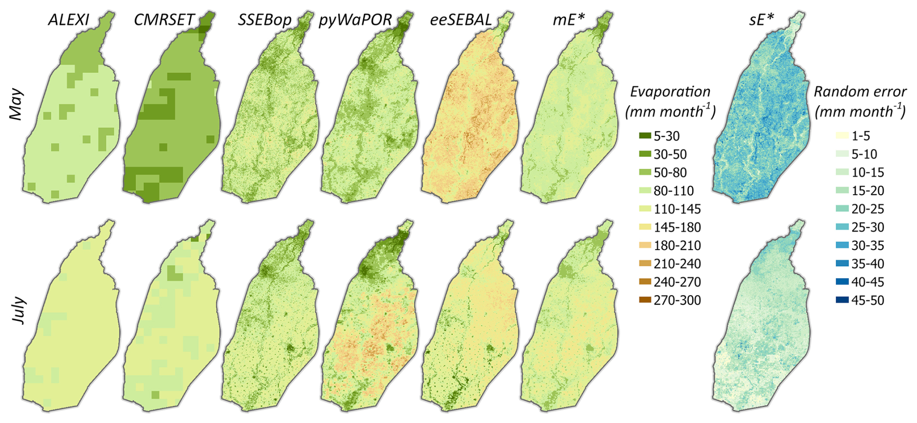
Figure 6 Prior observations and estimated posteriors of grid-scale evaporation E before the monsoon (May 2009) and for a peak rainy month (July 2009); ${\mathit{m}}_E^{*}$ and ${\mathit{s}}_E^{*}$ denote the posterior mean and standard deviation of evaporation.

In Fig. 7, we see that the precipitation posterior mean falls between the gridded precipitation data products. The spatial difference maps between the grid-scale observations and the posterior mean show that TRMM observes lower precipitation (by −60 to −35 mm month⁻¹), while MSWEP observes higher precipitation (by 25 to 48 mm month⁻¹) than the posterior mean. On the other hand, GPM deviates by −21 to 60 mm month⁻¹ from the posterior mean (Fig. C6 in Appendix C). As we have seen with the evaporation standard errors, the grid-scale posterior standard errors of precipitation are the highest at spatial locations where the difference across the products is the largest (upper part of the basin), and vice versa.

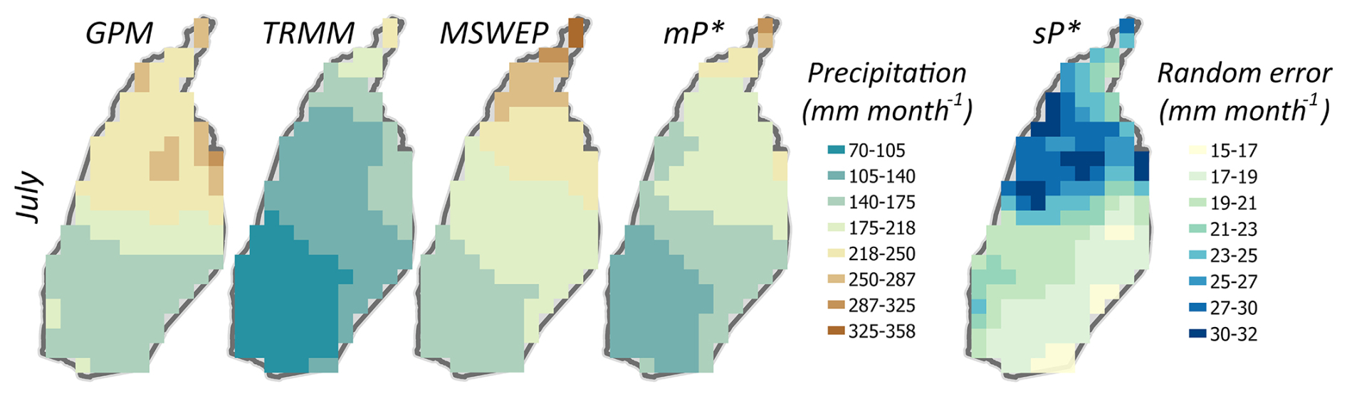
Figure 7 Prior observations and estimated posteriors of grid-scale precipitation P for the peak rainy month (July 2009); ${\mathit{m}}_P^{*}$ and ${\mathit{s}}_P^{*}$ denote the posterior mean and standard deviation of precipitation.

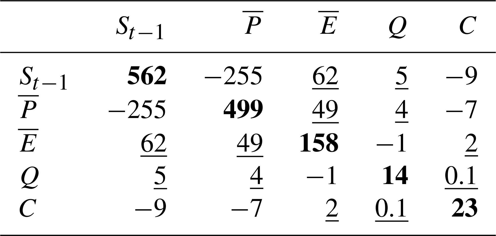
Via Eq. (29), the posterior cross-correlation between water variables at the basin scale is propagated to the grid scale, and thus results in posterior cross-correlation between grid-scale P and E as well. The effect of this can be illustrated by computing derived variables that involve both P and E. An example is given in Fig. 8, which shows maps of the posterior mean and standard deviation of P−E for July 2009, the latter with and without posterior cross-correlation between P and E. Due to positive posterior cross-correlation between P and E (since they have opposite signs in the water balance), the posterior standard deviation of P−E decreases when accounting for this correlation, but the effect in Fig. 8 is relatively small, and is observed at some localized spots with the highest reduction in errors of up to 2.5 mm month⁻¹. These spots correspond to the locations at which both P and E covary the most, with the cross-covariance subtracted during the computation of the P−E posterior variance. The reason for this relatively small effect is that the water balance constraints introduce other posterior cross-correlations as well, both at the basin scale (Table 2) and at the grid scale via nonlocal posterior cross-correlations between P and E induced by Eq. (29) (i.e., in the posterior, P in a grid cell becomes correlated with E in all other grid cells).

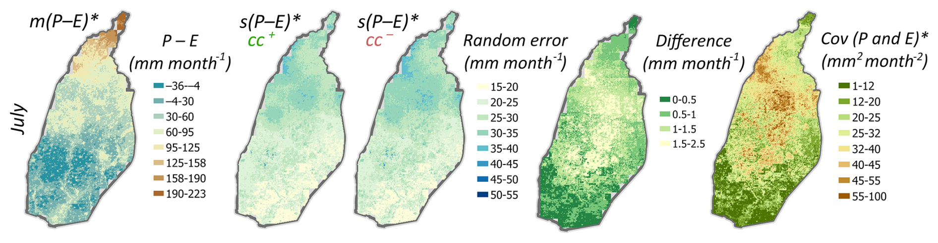
Figure 8 Grid-scale posterior mean ${\mathit{m}}_{P\text{-}E}^{\ast }$ and standard deviation ${\mathit{s}}_{P\text{-}E}^{\ast }$ of P−E, and P and E covariance for July 2009. The posterior standard deviations are computed for the two cases: with (cc⁺) and without (cc⁻) accounting for posterior cross-correlations (cc) between P and E, while the difference ${\mathrm{cc}}^{-}-{\mathrm{cc}}^{+}$ between these two cases illustrates the impact of accounting for cross-correlations.

To evaluate the effect of ignoring the posterior correlation between P and E, we calculated the distribution of Q from the water balance given the posterior of all other variables for three cases: (i) ignoring all posterior correlation, (ii) ignoring only correlation between P and E, (iii) accounting for all correlation. We compare these distributions to a fourth scenario (iv) in which Q is obtained from uncalibrated water balance data. Writing the water balance (Eq. 1) in terms of Q results in 15 uncalibrated Q estimates generated from the unique combinations of the water balance data. The distribution for this case is characterized in terms of mean (average across the 15 uncalibrated values) and uncertainty (set as the spread across these values). The results in Fig. 9 indicate that neglecting the posterior cross-correlation between P and E and between all water balance variables, can substantially lead to higher uncertainties (wider distributions), compared to when cross-correlations between all variables are accounted for (narrow distribution). At the extreme end, the Q predicted from the uncalibrated water balance data demonstrated the highest level of uncertainty compared to all other cases, with physically inconsistent values (negative) and a mean value greatly deviating from the observed Q value. We repeat this experiment for all months and report the performance of the estimated Q from the different approaches compared to the observed Q estimates. We obtain a low RMSE value of the calibrated Q posterior mean (0.7 mm month⁻¹) compared to Q_wb from uncalibrated water balance data (74 mm month⁻¹), which underscores the importance of (i) water balance data fusion for bias-correcting the original data products and (ii) accounting for posterior correlation, when water balance variables (P, E, C, S) are to be used for computing Q.

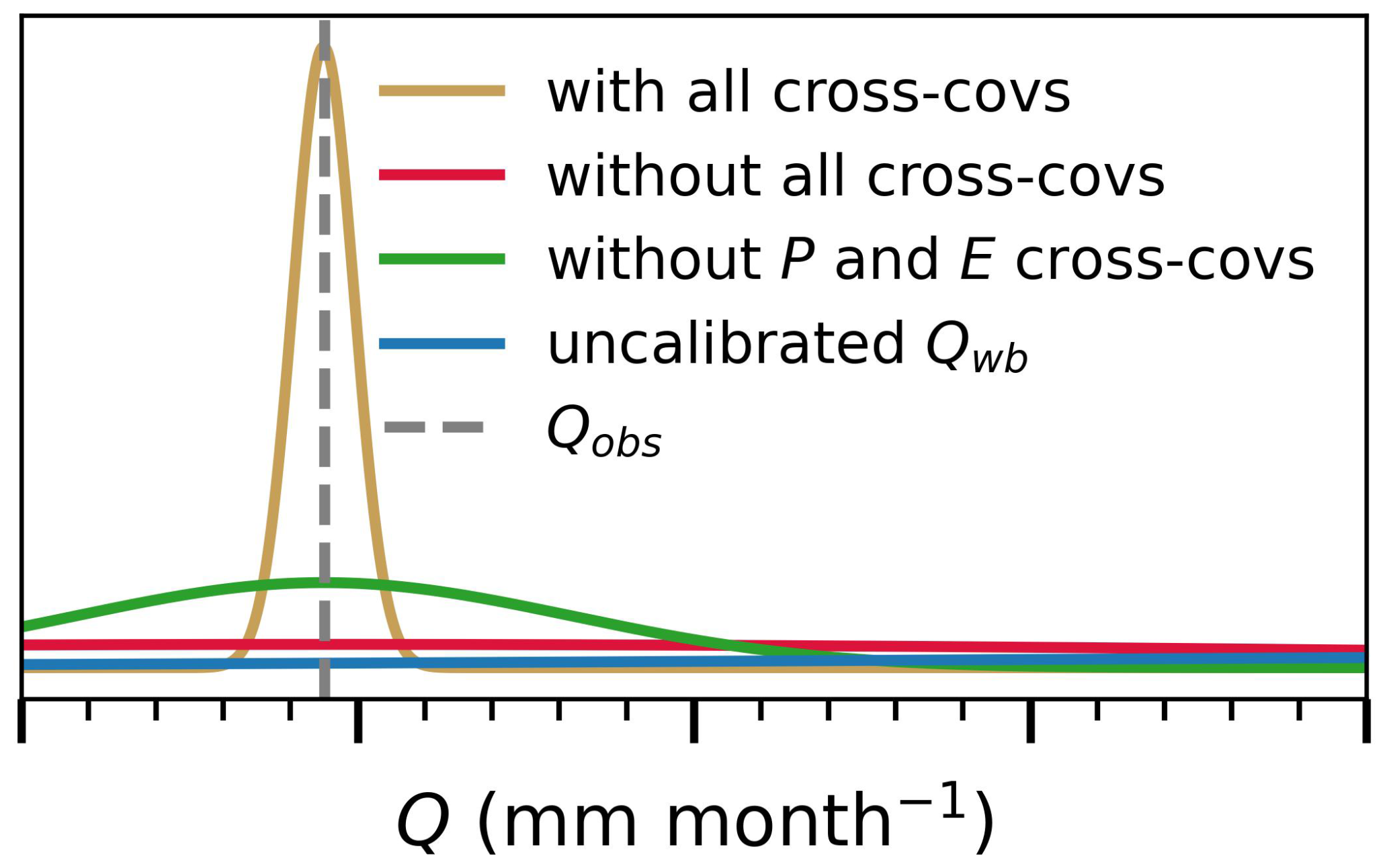
Figure 9 Distribution of Q in comparison to the observed Q_obs value (July 2009), for the following cases: (i) ignoring and accounting for posterior correlations between all water balance variables, (ii) ignoring only the posterior correlation between P and E, and (iii) Q_wb obtained from uncalibrated water balance data. The labels and tick marks are not shown due to data sharing restrictions.

Table 2 Basin-scale posterior covariance matrix of all water balance variables for July 2009, the diagonal elements represent the posterior variances (mm month⁻¹) (shown in bold), while the off-diagonal entries represent the posterior covariances between the variables (mm² month⁻²) (underlined values).

6 Discussion

This section evaluates some of the modeling decisions and their impact on the results, specifically the choice of GRACE data set and the choice of spatial correlation lengths of P and E.

6.1 Water balance data fusion with different GRACE data

The Hindon basin studied here is experiencing groundwater depletion (Alam and Umar, 2013). Storage data from GRACE satellite has been used to estimate human-driven water storage changes, such as those caused by intensive irrigation. This data is either based on spherical harmonic coefficients or mascon basis function, which entails testing the sensitivity of the water balance closure to the chosen GRACE input. The baseline results presented in Sect. 5 are based on GRACE-JPL Mascon (MAS) solution. Here, we compare these results to those obtained using the CSR spherical harmonic (SH) solution.

Figure 10 compares the posterior distributions for storage and error parameters from both data sets. The corresponding error parameter posteriors are compared in Fig. 4. The two products show negative depleting trends with widely varying magnitudes of −43.3 mm year⁻¹ from the SH and −88.7 mm year⁻¹ from MAS. Looking at their corresponding posterior distributions, we can see that they both largely follow the GRACE data, but with an increase in the seasonal amplitude compared to the data. This is reflected in the inferred A parameter (row 2 in Fig. 4), with an estimated value of 90–100 mm for both cases. The storage posteriors, thus, restore the seasonal signal amplitude, which tends to be more severely attenuated in small-sized basins like the Hindon basin. Additionally, the other storage error parameters (phase δ and noise σ_S) distributions are well constrained compared to their vague prior distributions. A relatively small phase error (time lag) is obtained using the two data sets. However, the JPL-MAS data yields a smaller noise (53 mm) than the CSR-SH (60 mm) data. The fact that these error parameters are time-invariant and that the posteriors are computed using data from all months via iterative smoothing allows the probabilistic water balance model to fill in the data gaps present in GRACE data sets from 2011 onwards.

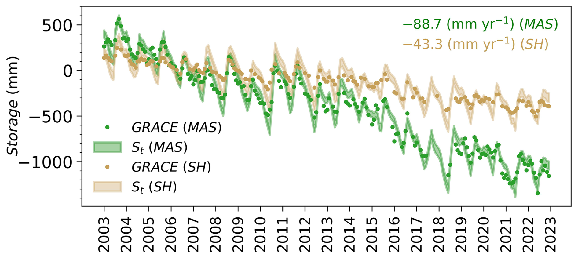
Figure 10 Storage posteriors for two different GRACE data sets: GRACE-JPL Mascon (MAS) and CSR spherical harmonic (SH) solution.

Figure 4 also depicts the posterior distribution of the precipitation and evaporation error parameters for the two scenarios. The water balance data fusion run with the CSR spherical harmonic (SH) solution gives more weight to the lower precipitation and evaporation estimates. This is translated into the w_P value of 0.15. Despite that, the posterior evaporation mean lay between the data limits (w_E=0.5) for this case, the bias scaling factor (f_E) masked out its effect (with estimated values smaller than 1), pushing the E posterior towards the lower evaporation end (i.e., the baseline evaporation limit). Figure C7 in Appendix C contains the detailed posterior plots for the water balance variables using the GRACE-SH data sets. Apparently, the GRACE-SH data set's storage dynamics don't match the other water balance variables in terms of water balance closure, at least with the applied P and E error models. Due to the smaller decreasing trend in the GRACE-SH storage data, the inferred evaporation estimates are, on average, about 15 % lower than the estimates obtained with the GRACE-MAS data. To consistently compare the data fit from both solutions, we normalize the likelihood by the number of observations in each data set. Consequently, the water balance model with GRACE-MAS data has a slightly larger likelihood (−5.76) than that with GRACE-SH (likelihood −6.0).

This analysis suggests that long-term groundwater depletion in the basin is possibly better captured by the (more severely declining) mascon data, which has important ramifications for the sustainability of irrigation practices in the basin. This conclusion, however, requires further verification with groundwater level trends from piezometer data.

6.2 Sensitivity to the assumed spatial correlation length-scale parameters

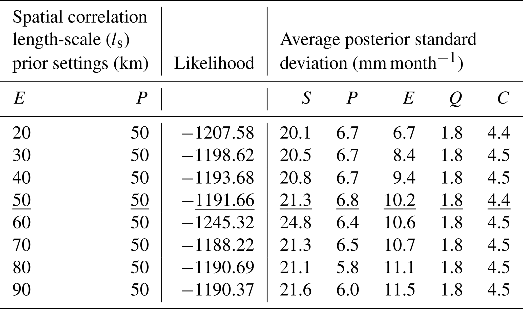
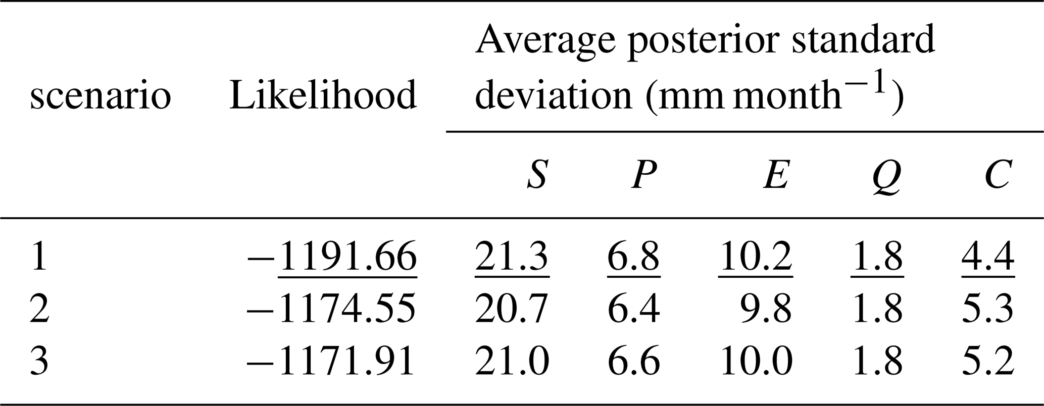
The posterior results in the preceding section are obtained by running the water balance data fusion with fixed Matérn parameters for both the evaporation and precipitation processes. Given the differences in spatial resolution of the analyzed data, the smoothness and correlation length-scale l_s were specified with mid-range values of 1.5 and 50 km, respectively. To evaluate the sensitivity of the results to the chosen value for l_s, we set the value of precipitation l_s at 50 km and vary that of evaporation, and vice versa. Table 3 lists these prior conditions, along with the likelihood and average posterior standard deviation for each water balance variable. The results show stability of the posteriors and the likelihood values under all prior settings, except for the cases where precipitation and evaporation l_s are low (e.g., 20 km). In these cases, the probabilistic water balance exhibits the poorest fit to the data (i.e., small likelihood values), and the basin-scale posterior uncertainty of either evaporation or precipitation tends to be underestimated. On the other hand, using mid-range to larger spatial correlation length scale values produces slightly different but substantively comparable posteriors and likelihood values. The relative insensitivity to l_s suggests its value could potentially be chosen to a very large value to speed up the computations: in the limit of perfect spatial correlation, the formulas linking grid and basin scales simplify, which can result in much faster computations for large grids.

Table 3 Average posterior standard deviation (mm month⁻¹) for each water balance variable and likelihood values under different spatial correlation length-scale (l_s) prior settings. The underlined values represent the results of the baseline setup of the water balance data fusion model, with GRACE-JPL Mascon data set and fixed correlation length scale at 50 km.

6.3 Sensitivity of the posteriors to the prior canal water import estimates

The baseline results presented in Sect. 5.1 are based on the canal water import data generated using a combination of canal design capacities multiplied by their operational time, and the data average of years with similar conditions (Appendix A, Sect. A2). Here, we evaluate the sensitivity of the probabilistic water balance model to the different approaches used to generate canal water estimates from little available data, compared to the one adopted in the baseline run (we refer to it here as scenario 1). To do so, we include two additional scenarios, one in which the prior canal estimates are computed using only the canal design capacities multiplied by their operational time obtained from irrigation schedules (scenario 2), and the other is based on the assumption that the total flows into the basin are 20 % of the monthly flows in the UGC main canal (scenario 3). For this evaluation, we assess the model fit given the data (likelihood value) and the average posterior standard deviation (mm month⁻¹) for each water balance variable. The resulting water balance variables posteriors showed minimal variations with the different water supplies prior estimates (Table 4). Although the fit is better with scenarios 2 and 3, the posterior error for this term is the lowest for scenario 1. Generally, this analysis shows an insensitivity of water balance posteriors to the canal water data used, and indicates that the prior estimates presented in Sect. 5.1 are sufficient for the goal of constraining the other water balance variables.

Table 4 Average posterior standard deviation (mm month⁻¹) for each water balance variable and likelihood values with different canal water import prior estimates. The underlined values represent the results of the baseline setup of the water balance data fusion model, with GRACE-JPL Mascon data set and fixed correlation length scale at 50 km.

6.4 Extensions

The presented methodology is motivated by the availability of diverse water balance remote sensing data, with very few in situ data available for the Hindon basin, making independent validation of our estimates challenging. For this reason, we evaluated our results using soft validation techniques. For example, for evaporation, in the absence of in situ data, we compared the trend in our estimated evaporation with independent crop yield data, and the seasonal dynamics with known cropping and irrigation patterns (see Sect. 5.1). As for the precipitation posterior estimates, in Sect. 5.1 and Appendix C, these were compared to the spatially interpolated rain gauge dataset for the basin from the Indian Meteorological Department (IMD), keeping in mind the potential underestimation of precipitation by this dataset (Goteti and Famiglietti, 2024). Evaluating the total water storage estimates with independent data is more challenging. In a follow-up study, we will introduce separate rootzone and groundwater balance constraints, with the aim of estimating their contributions to the total water balance. At that point, it will become possible to use available remote sensing soil moisture data, as well as in-situ groundwater level data, for evaluation. Furthermore, adding these additional constraints and data will allow for updating the posterior estimates in this paper.

Additionally, the presented methodology is general and can be applied to other gauged river basins. For example, an application to multiple semi-arid basins was reported in Schoups and Nasseri (2021). The method has several advantages that allow this, including the straightforward and flexible implementation, as it consists of two separate parts: error models specification for each water balance variable that can be customized to fit specific settings, and the model solver that automatically computes the posterior distributions. In addition, the method is set up to rely on in situ and satellite data that inherently capture the hydrological processes. For example, the precipitation data sets estimate the precipitation phase (snow and rain), while evaporation data sets can be used to differentiate between the different land use classes. However, in snow-dominant basins where precipitation data sets might underrepresent this process, or in urban-dominant settings where coarse-resolution evaporation data products might overestimate evaporation, it may be valuable to tailor the error models to local conditions in order to improve the results. Perhaps, this could be achieved by complementing the precipitation error models with other satellite data sets, like the snow cover, snow depth, or temperature products, for better snow detection and mapping. Moreover, evaporation error models can be complemented with land use maps while also considering the use of high-resolution evaporation products or other data sets with improved evaporation estimates of heterogeneous urban surfaces. The major assumption here is that formulating the error models by exploiting ancillary information would allow it to solve for error parameters and water balance variables under varying climatic zones and settings. Alternatively, for this purpose, we could combine the data error models with hydrological models that explicitly account for detailed processes and differentiate between the different hydrological responses.

7 Conclusions

This paper presents a multi-scale monthly probabilistic water balance data fusion model for calibrating estimates of each component of the water balance. A key contribution of this paper is the calibration of gridded precipitation and evaporation estimates in an ensemble approach that fully exploits the prior information content of the data. To achieve this, the introduced methodology is applied at two scales: the basin scale and the grid scale. First, we formulate prior grid-scale and ensemble-based error models for precipitation and evaporation with unknown error parameters that describe the bias and random errors in their spatial fields. The spatially averaged inputs to the precipitation and evaporation error models, along with in situ data (river discharge and canal imports) and storage data from GRACE, then drive a basin-scale probabilistic water balance closure approach. In this approach, the water balance is treated as a Bayesian model by assigning prior distributions with unknown bias and noise parameters to each water balance variable. Combining these prior distributions with monthly water balance constraints results in posterior estimates of all parameters and variables that jointly close the water balance at the basin scale. The resulting basin-scale precipitation and evaporation posteriors and their cross-correlations are then used to update the prior grid-scale data from the first step. This is attained using a Kalman smoothing algorithm that ensures consistency between the grid-scale and the basin-scale estimates; that is, spatially averaging the calibrated gridded estimates yields monthly precipitation and evaporation values that jointly satisfy the water balance at the basin scale together with the other variables (C, Q, S).

We apply the introduced methodology to the Hindon Basin, a tributary of the Yamuna River that suffers from unsustainable irrigation practices relying on the local groundwater and imported surface water. The basin-scale results demonstrate that introducing an independent set of in situ data on surface water imports and river discharge, along with monthly water balance constraints, updates the prior information with new information, automatically adjusts different information sources for each water balance variable, while maintaining a closed water balance. The output of this study highlights the potential of the monthly water balance constraints in substantially reducing uncertainties by accounting for cross-correlations between all water balance variables. In addition, the model yields basin-wide posterior estimates of: (a) error parameters that are well constrained by all water balance data, and (b) consistent basin-scale water balance variables that jointly close the water balance. Transferring these basin-scale constraints to the grid scale results in: (a) posterior ensemble mean of precipitation and evaporation that fuses the pixel-wise information from extreme prior data bounds (min-max) and finds a balance between the two according to their relative errors, and (b) posterior random errors that reflect the model confidence about the location of the posterior mean at each grid cell.

Explicit to the introduced approach are the assumptions made about the data to characterize their associated errors in a parametric form. For instance, a range-based error model is used to quantify errors in the gridded precipitation and evaporation data. Here, the bias error is described as a weighted average of the minimum and maximum estimates at each spatial location. Whereas, the random error is quantified by scaling the maximum potential error (i.e., scaling one-quarter of the grid-scale full range). As an extension to this analysis, alternative data error models might be worth considering. E.g., a possible alternative is to use Gaussian mixture models that calibrate each data set individually, while still exploiting the water balance as a constraint.

As for the errors in a single GRACE data set, these are modeled using a noisy sine wave error model with unknown phase and amplitude error parameters that are used to correct for the dominant biases in the GRACE data (i.e., leakages). The sensitivity of the model results to the input data is assessed using two GRACE data sets: spherical harmonic (GRACE-CSR) and mascon solution (GRACE-JPL). This is done quantitatively by comparing the values of the inferred noise parameters (a smaller value is preferred) and that of the likelihood, as a larger likelihood corresponds to a better fit. While the GRACE-JPL demonstrated a better performance than GRACE-CSR based on these evaluation criteria, this could also be influenced by the assumptions surrounding the precipitation and evaporation error models. Ground-based piezometer data may also help resolve the difference between the downward trends in the two GRACE data sets for the studied basin, which is important for evaluating the sustainability of irrigation practices in the basin.

Finally, the random errors in the monthly river discharge and canal water import data are more or less fixed to relative errors. A larger prior uncertainty is assigned to the gap-filled canal import data (25 %) than to the river discharge (10 %). Regardless of the approach used to generate prior canal water import estimates from little available data, these were sufficient to constrain the other water balance terms. Additionally, the generated water balance estimates are not strongly affected by the assumed errors for the canal water and river discharge data, as these two variables are relatively small compared to the other monthly water balance variables (especially during rainy months when the two processes are driven by precipitation). We also examined the impact of fixing the spatial correlation length scale parameter on model fit and the posterior standard errors. The posterior results showed robustness and model fit improvement across mid-to-large values of prior parameter sets. This suggests that this parameter does not influence the model results in a large way.

A key aspect of the proposed methodology is that it is data-driven, exploiting the water balance constraint as an independent source of information. Therefore, the resulting calibrated data generated here can be used as baseline data sets for multiple applications, such as the validation or calibration of hydrological models, climate studies, and water accounting assessments. Nonetheless, updating the calibrated and spatially distributed estimates of precipitation and evaporation, and storage data generated herein with constraints describing the physical relations between detailed water balance variables (e.g., vertical and horizontal flows), along with additional in situ data (e.g., groundwater storage observations from piezometers), hold a great premise for synergetic and complementary use of all information sources. This will be the scope of a follow-up study for the investigated basin that aims to constrain water balance stocks and flows and their errors using grid-scale water balance constraints.

Appendix A: Additional data

The following subsections summarize the available information on the Hindon basin land use elements (Fig. A1), share of canal water imports in the water balance (Fig. A2), canal network (Figs. A3 and A4), its operation, irrigation canal delivery data, and processing steps.

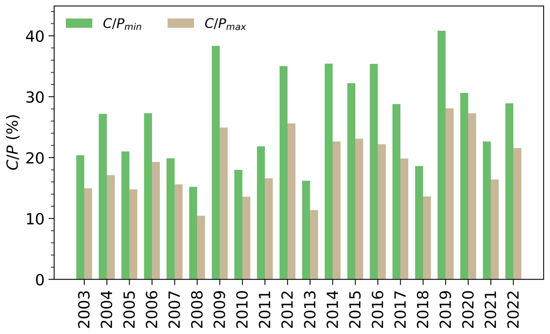
Figure A1 Share of the canal water imports in the water balance, expressed as the percentage of the minimum and maximum remote sensing-based precipitation observations.

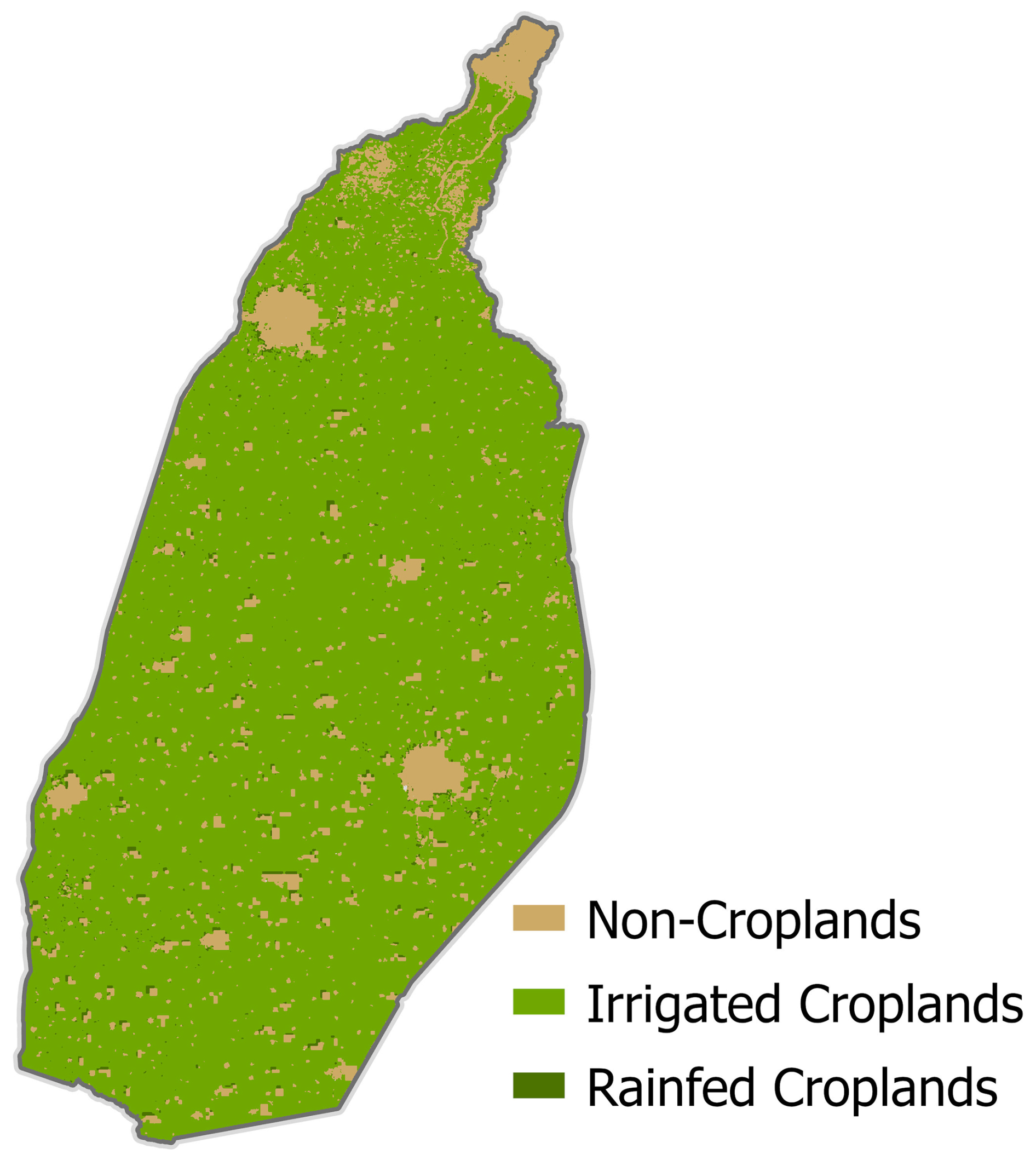
Figure A2 Land use elements distribution in the Hindon basin from Gumma et al. (2022).

A1 Description of the canal irrigation system and its operation

Figures A3 and A4 provide an overview of the canal network's spatial distribution and design capacities. While these main canals run continuously, their distributaries are operated in rotation (Ahmad, 1991; Chaube et al., 2023). The canal distributaries in the Hindon basin are operated on an “on-off” basis as shown in Table A1. The irrigation schedules (also known as the rosters) are prepared for two irrigational seasons:

1. Kharif season in which the main irrigated crops are sugarcane, rice, cotton, maize, vegetables, and fodder crops

2. Rabi season in which the principal crops are wheat, barley, mustard, and peas.

Table A1 Example of seasonal operational schedule (the ON-OFF basis) for Eastern Yamuna Canal (EYC) and Upper Ganga Canal (UGC) distributaries. Kharif spans from March to September 2021, while Rabi covers Oct 2021 to March 2022.

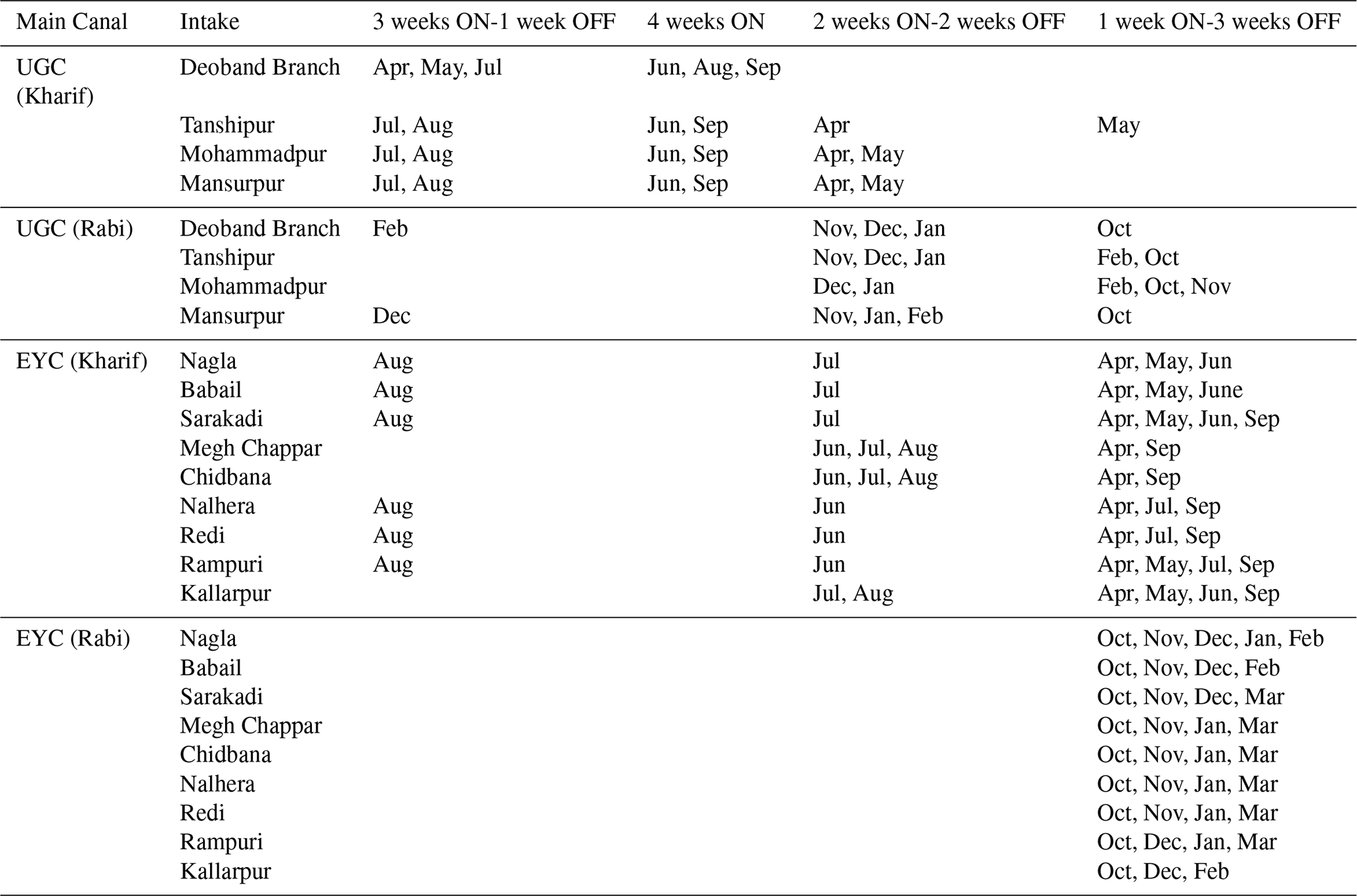
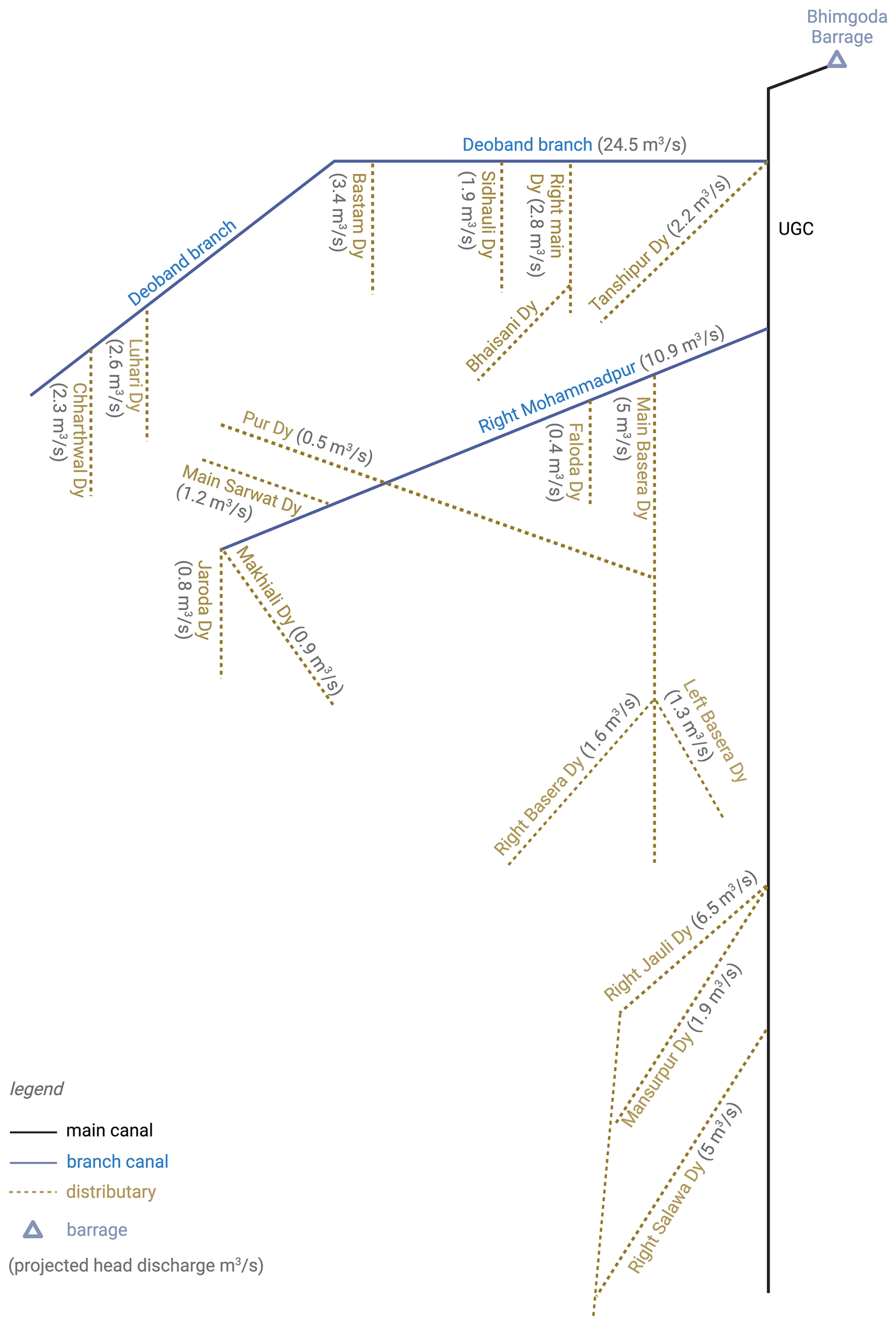
Figure A3 A schematic of the UGC main canal and its distributaries with their respective discharge capacities (m³ s⁻¹).

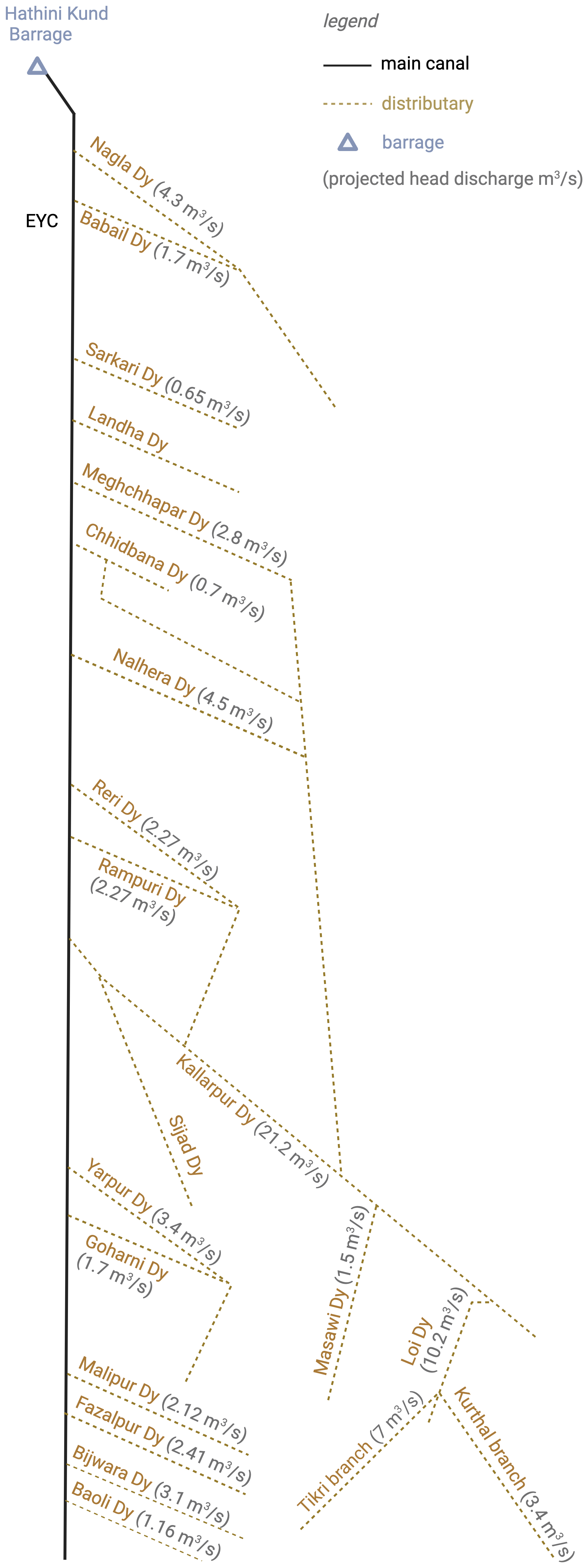
Figure A4 A schematic of the EYC main canal and its distributaries with their respective discharge capacities (m³ s⁻¹).

A2 Description of irrigation canal delivery data and processing steps

Constrained by the limited availability of data on water deliveries, we use an extrapolation approach to fill in the data gaps. The approach integrates two data sources, the irrigation schedules and the actual flow measurements from in-situ data, to produce a complete monthly timeseries. Explicit in this method is the assumption that the canal operations do not vary widely between years in which the conditions are similar. For instance, if years “A”, “B”, and “C” are classified as “dry years,” the canal operations don't differ much across these years. In other words, if year “A” has unknown estimates, these can be estimated from year “B” or the mean of the three years, depending on the number of years with canal data. Therefore, each group of distributaries is filled out based on two criteria: the data source and the number of years with available data. For the canals, such as the Deoband parallel, with actual flow measurements and ≥5 years of data availability, we solely rely on these data for extrapolation. To this end, we distinguish the years into three conditions (wet, dry, and normal years) using the Palmer Drought Severity Index (PDSI) Terra climate data set as a proxy. Then, every unknown year is filled with the long-term average of the years falling under the same category. For example, when a year such as 2015 is identified as “normal”, this year is filled with the mean of the canal delivery observed across all other “normal” years. A similar procedure was applied to the EYC lower intakes with actual flows from 2018 to 2022 to fill in missing data for similar years outside this period. For the other intakes with only a few years of data, however, we filled them differently. For instance, the lower intake points of the UGC with flow measurements for only two years, 2021 (dry) and 2022 (wet), we use these years as benchmarks for filling similar wet or dry years. For “normal” years on these intakes, we use the irrigation schedules instead. Explicitly, in cases with only a single-year irrigation schedule, the flows are obtained by multiplying the full design capacity by the operational time. This step produces conservative and monthly variable flow estimates due to the operational time variation of each distributary. Since the Deoband branch contributes a significant share of the total canal water supplies into the basin, we fill its missing data using the irrigation schedules to avoid the impacts of assuming no variation in operation across the years. In cases where single-year data is available for distributaries such as Bijwara and Baoli, we use the actual flows for this year (2018) as a reference to fill all other years. As for distributaries without data from design or actual flows, we assume these might not add much to the overall imports into the Hindon basin. At this stage, the canal delivery data is at the daily timestep. The last step is to aggregate to a monthly timescale, sum all intakes, and normalize by the basin area to obtain the gap-filled canal water imports expressed in water depth units (mm month⁻¹).

Table A2 Available information on the distributaries and their coverage. The data source column distinguishes between actual (measured) and planned (scheduled) irrigation canal delivery data.

Appendix B: Additional methods

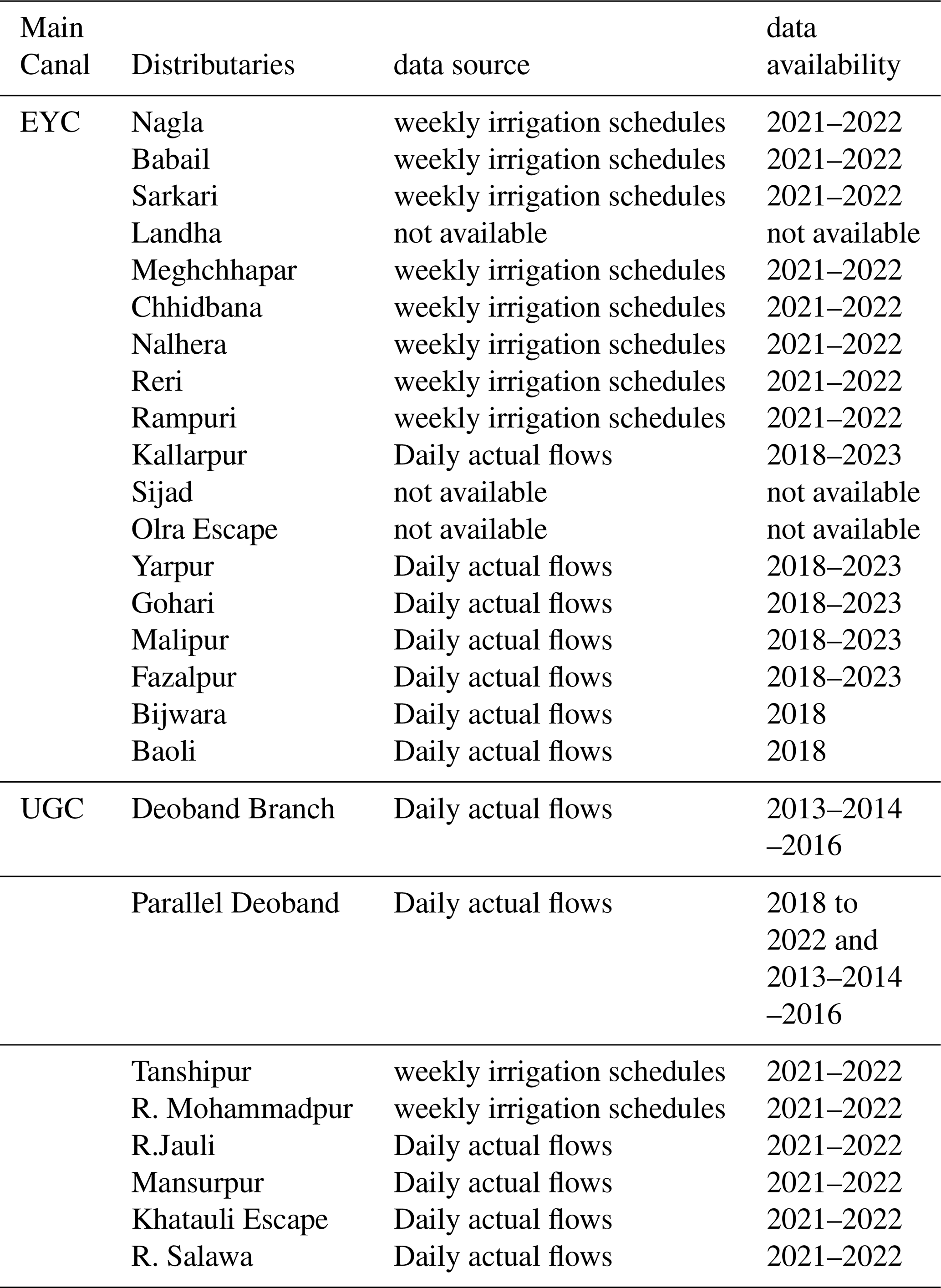
B1 A major challenge arising from the use of uncalibrated remote sensing water balance data

The following figure shows that imbalance errors due to combining uncalibrated remote sensing products for each water balance variable can be significant ($\sim \pm \mathrm{200}$ (mm month⁻¹)). This is related to errors associated with the data. Therefore, there is a need to quantify and reduce these uncertainties.

B2 Computing posteriors of individual variables, parameters, and posterior cross-correlations between water balance variables

This section briefly explains how all posteriors are computed. For the probabilistic water balance model described in Sect. 4.1 of the main text, we can represent its joint distribution as $p(x,\mathit{\theta },S_{\mathrm{obs}})$. This distribution consists of two parts: the monthly water balance variables x (comprising 5N + 1 variables including S₀, ${\stackrel{\mathrm{‾}}{P}}_t$, ${\stackrel{\mathrm{‾}}{E}}_t$, Q_t, C_t and S_t), where N is the number of months and is equal to 240 for 20 years of data considered in this paper, S₀ is the initial basin water storage at the start of the first month and S_obs is the storage timeseries, and the parameter vector θ, including w_P, r_P, w_E, f_E, r_E, a_Q, b_Q, a_C, b_C , σ_S, A, and δ. Our objective is to compute the full posterior distribution, which integrates all available information sources (Gaussian distributions) of θ and x.

The posterior of the parameter vector is expressed in the following form:

$$\begin{array}{}\text{(B1)}& p\left(\mathit{\theta }\mathrm{|}{S}_{\mathrm{obs}}\right)\propto p\left(S_{\mathrm{obs}}\mathrm{|}\mathit{\theta }\right)p\left(\mathit{\theta }\right)\end{array}$$

where p(θ) is the prior distribution for the parameters and corresponds to the product of the individual parameter priors defined in the previous basin-wide error model section, while the term p(S_obs|θ) refers to the parameter likelihood function. This function scores each set of bias parameters (e.g., w_E, f_E) and noise parameters (e.g., r_E,σ_S). A large likelihood for the parameters is one that shifts the storage predicted from the water balance closer to the storage observations. As we show below, this likelihood also connects the DE-MCMC for parameter sampling and EP for posterior computations of water balance variables.

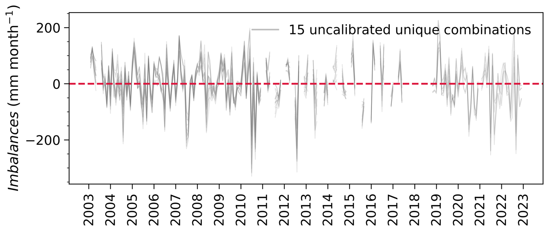
Figure B1 Monthly timeseries of the imbalances (water balance errors) for each of the 15 unique uncalibrated combinations of the variables.

In the basin-wide inference setup, an outer MCMC loop iteratively proposes sets of parameter candidates (samples) using a non-parametric proposal (jumping) mechanism (Ter Braak and Vrugt, 2008). For each set of sampled parameters by MCMC, the EP (message passing) algorithm operates in an inner loop, computing the (a) unnormalized posterior density of the parameters proposed by MCMC (Eq. B1) and the conditional water balance posteriors $p\left(x\right|S_{\mathrm{obs}},\mathit{\theta })=\frac{p\left(x,S_{\mathrm{obs}}|\mathit{\theta }\right)}{p\left(S_{\mathrm{obs}}|\mathit{\theta }\right)}$. The normalizing constant of the conditional water balance posterior (p(S_obs|θ)) is the likelihood in Eq. (B1). EP evaluates the posterior odds of the model outputs $p\left(x\right|S_{\mathrm{obs}},\mathit{\theta })$ given the sampled parameters, guiding the DE-MCMC decisions in accepting or rejecting new parameters. Compared to the standard single forward-backward algorithm, EP approximates the exact posterior distributions with Gaussian distributions sharing matching moments (mean and variance). It involves multiple back-and-forward passes over the data using the entire timeseries until all posteriors stabilize. A key aspect of the EP algorithm is its ability to efficiently handle non-Gaussian posteriors, which arise from physical non-negativity constraints we force on water balance variables ($\stackrel{\mathrm{‾}}{P}$, $\stackrel{\mathrm{‾}}{E}$, Q, C). Typically, a small number of iterations are sufficient to achieve convergence due to the mild non-Gaussianity induced by these constraints. The EP algorithm yields conditional water balance posteriors (conditioned on the S_obs data and the parameter vector θ). Instead of the conditional posterior distribution, we are interested in the marginal posterior distribution p(x|S_obs) over the individual water balance variables (S₀, $\stackrel{\mathrm{‾}}{P}$, $\stackrel{\mathrm{‾}}{E}$, Q, and C). Such distributions are obtained by integrating (∼ averaging) $p\left(x\right|S_{\mathrm{obs}},\mathit{\theta })$ over the parameter posterior distribution p(θ|S_obs), effectively accounting for the parameter uncertainty in the final water balance estimates:

$$\begin{array}{}\text{(B2)}& \mathrm{p}\left(x\mathrm{|}{S}_{\mathrm{obs}}\right)=\int p\left(x\right|S_{\mathrm{obs}},\mathit{\theta }\left)p\right(\mathit{\theta }\mathrm{|}{S}_{\mathrm{obs}})d\mathit{\theta }\end{array}$$

This paragraph explains how to compute posterior cross-covariances between the different water balance variables given the posterior marginal distributions of each variable (as output by the water balance data fusion model). For this, we will need two building blocks to construct the joint precision matrix (Θ) equal to the inverse of the covariance matrix (V^∗), namely: the variables' linear relation through the water balance coefficients $\mathit{\phi }=\left[\mathrm{1},\mathrm{1},-\mathrm{1},-\mathrm{1},\mathrm{1}\right]$ extracted from the water balance constraint at each time step: $S=S_{\mathrm{0}}+\stackrel{\mathrm{‾}}{P}-\stackrel{\mathrm{‾}}{E}-Q+C$ and “uncorrelated priors” of each variable. The term “priors” reflects uncertainty before considering the relation of each variable with other variables. With the marginal distributions available at this point, we can back-calculate these priors such that they satisfy the marginals through a message-passing algorithm. This algorithm relies on decomposing the marginal precisions (τ) for each variable into: (a) prior precisions (messages) for each variable and (b) precisions (messages) sent to each variable from all other variables via the water balance. Specifically, in each month, we have two conditions: the water balance constraint and the probabilistic constraints in the form of marginal Gaussian distributions written separately for individual variables x as $p\left(x\right)\sim \mathcal{N}\left(m_x^{\ast },v_x^{\ast }\right)$, with posterior mean and variance obtained from Eq. (27) in the main text. Expressed in terms of precisions, we can write the decomposed posterior precision of S (τ_S), for example, as: ${\mathit{\tau }}_S={\mathit{\tau }}_{S\to }+{\mathit{\tau }}_{\to S}$ where τ_S→ is the prior precision from S, and τ_→S is the precision to S from the water balance. The latter can be obtained from all other variables by propagating uncertainty through the linear water balance equation. As such, the relationship between the posterior and prior variances of S that fulfill the two defined conditions becomes:

$$\begin{array}{}\text{(B3)}& {\displaystyle \frac{\mathrm{1}}{v_S^{\ast }}}={\displaystyle \frac{\mathrm{1}}{v_{S\to }}}+{\displaystyle \frac{\mathrm{1}}{v_{S_{\mathrm{0}\to }}+v_{{\stackrel{\mathrm{‾}}{P}}_{\to }}+v_{{\stackrel{\mathrm{‾}}{E}}_{\to }}+v_{Q\to }+v_{C\to }}}\end{array}$$

We can repeat the above step for all other variables to create a linear system of six equations with six unknowns (prior variances) that we need to solve for:

$$\begin{array}{}\text{(B4)}& \left\{\begin{array}{l}\frac{\mathrm{1}}{v_S^{\ast }}-\frac{\mathrm{1}}{v_{S\to }}-\frac{\mathrm{1}}{v_{S_{\mathrm{0}\to }}+v_{{\stackrel{\mathrm{‾}}{P}}_{\to }}+v_{{\stackrel{\mathrm{‾}}{E}}_{\to }}+v_{Q\to }+v_{C\to }}=\mathrm{0}\\ \frac{\mathrm{1}}{v_{S_{\mathrm{0}}}^{\ast }}-\frac{\mathrm{1}}{v_{S_{\mathrm{0}}\to }}-\frac{\mathrm{1}}{v_{S\to }+v_{{\stackrel{\mathrm{‾}}{P}}_{\to }}+v_{{\stackrel{\mathrm{‾}}{E}}_{\to }}+v_{Q\to }+v_{C\to }}=\mathrm{0}\\ \frac{\mathrm{1}}{v_{\stackrel{\mathrm{‾}}{P}}^{\ast }}-\frac{\mathrm{1}}{v_{{\stackrel{\mathrm{‾}}{P}}_{\to }}}-\frac{\mathrm{1}}{v_{S_{\mathrm{0}\to }}+v_{\to S}+v_{{\stackrel{\mathrm{‾}}{E}}_{\to }}+v_{Q\to }+v_{C\to }}=\mathrm{0}\\ \frac{\mathrm{1}}{v_{\stackrel{\mathrm{‾}}{E}}^{\ast }}-\frac{\mathrm{1}}{v_{{\stackrel{\mathrm{‾}}{E}}_{\to }}}-\frac{\mathrm{1}}{v_{S_{\mathrm{0}\to }}+v_{{\stackrel{\mathrm{‾}}{P}}_{\to }}+v_{S\to }+v_{Q\to }+v_{C\to }}=\mathrm{0}\\ \frac{\mathrm{1}}{v_Q^{\ast }}-\frac{\mathrm{1}}{v_{Q\to }}-\frac{\mathrm{1}}{v_{S_{\mathrm{0}\to }}+v_{{\stackrel{\mathrm{‾}}{P}}_{\to }}+v_{{\stackrel{\mathrm{‾}}{E}}_{\to }}+v_{S\to }+v_{C\to }}=\mathrm{0}\\ \frac{\mathrm{1}}{v_C^{\ast }}-\frac{\mathrm{1}}{v_{C\to }}-\frac{\mathrm{1}}{v_{S_{\mathrm{0}\to }}+v_{{\stackrel{\mathrm{‾}}{P}}_{\to }}+v_{{\stackrel{\mathrm{‾}}{E}}_{\to }}+v_{Q\to }+v_{S\to }}=\mathrm{0}\end{array}\right.\end{array}$$

Where $v_S^{\ast },v_{S_{\mathrm{0}}}^{\ast },v_{\stackrel{\mathrm{‾}}{P}}^{\ast },v_{\stackrel{\mathrm{‾}}{E}}^{\ast },v_Q^{\ast },v_C^{\ast }$ are the posterior marginal variances of the variables: Storage S, initial storage state for the first month S₀, $\stackrel{\mathrm{‾}}{P}$, $\stackrel{\mathrm{‾}}{E}$, Q, and C, respectively. While, $v_{S\to },v_{S_{\mathrm{0}\to }},v_{{\stackrel{\mathrm{‾}}{P}}_{\to }},v_{{\stackrel{\mathrm{‾}}{E}}_{\to }},v_{Q\to }$ and v_C→ are their corresponding prior variances.

The resulting priors are used to generate the joint precision matrix Θ of S₀, P, E, Q, and C, which combines two terms:

$$\begin{array}{}\text{(B5)}& \begin{array}{rl}& \mathbf{\Theta }\mathbf{=}\mathit{\phi }{\mathit{\phi }}^{{}^{\prime }}{\mathit{\tau }}_{S\to }+\mathrm{diag}\\ & \left(\left[{\mathit{\tau }}_{S_{\mathrm{0}}}\mathrm{or}{\mathit{\tau }}_{S_{t-\mathrm{1}}\to },{\mathit{\tau }}_{{\stackrel{\mathrm{‾}}{P}}_{\to }},{\mathit{\tau }}_{{\stackrel{\mathrm{‾}}{E}}_{\to }},{\mathit{\tau }}_{Q\to },{\mathit{\tau }}_{C\to }\right]\right)\end{array}\end{array}$$

The first term represents a matrix that encodes how each variable varies with every other variable in the water balance. This term is scaled by the prior precision from S (τ_S→), whereas the second term is a diagonal matrix of the other individual water balance variables prior precisions. The inverse of the joint precision matrix gives the posterior covariance matrix between all variables (in a given month), which contains all posterior cross-correlations.

Appendix C: Additional results

C1 Water balance priors and posteriors

This section displays the results of the seasonal and annual posterior means of the water balance variables compared to their corresponding prior data.

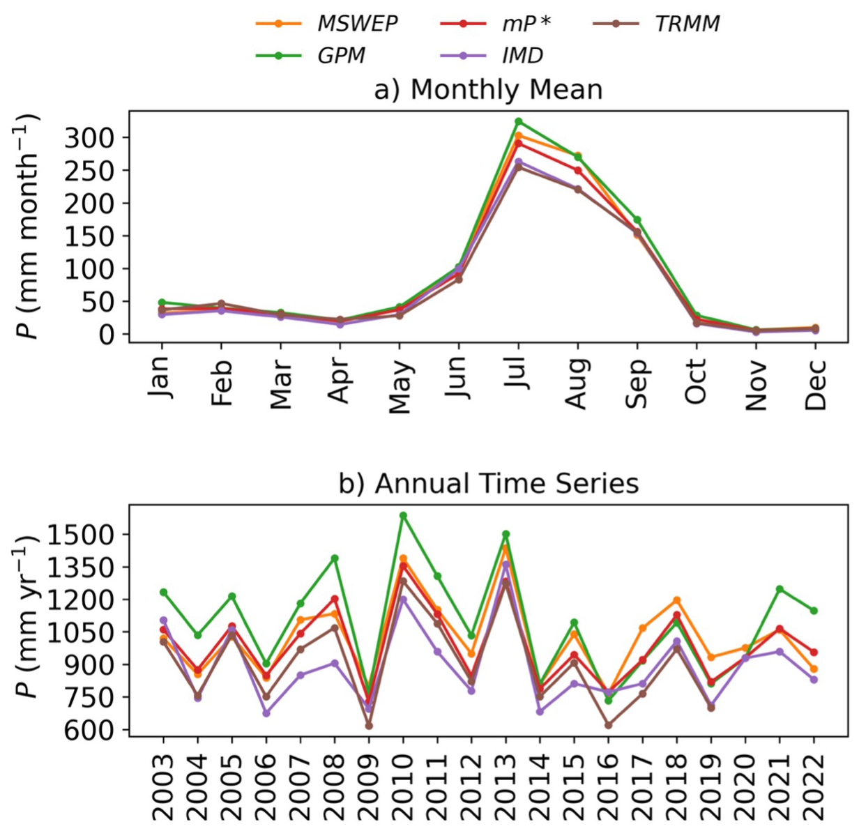
Figure C1 Comparison of posterior mean ($m_P^{*}$) to the prior data sets describing the precipitation (P) variable in the Hindon basin, the top panel depicts (a) monthly mean P, and the bottom panel (b) shows the annual P time series.

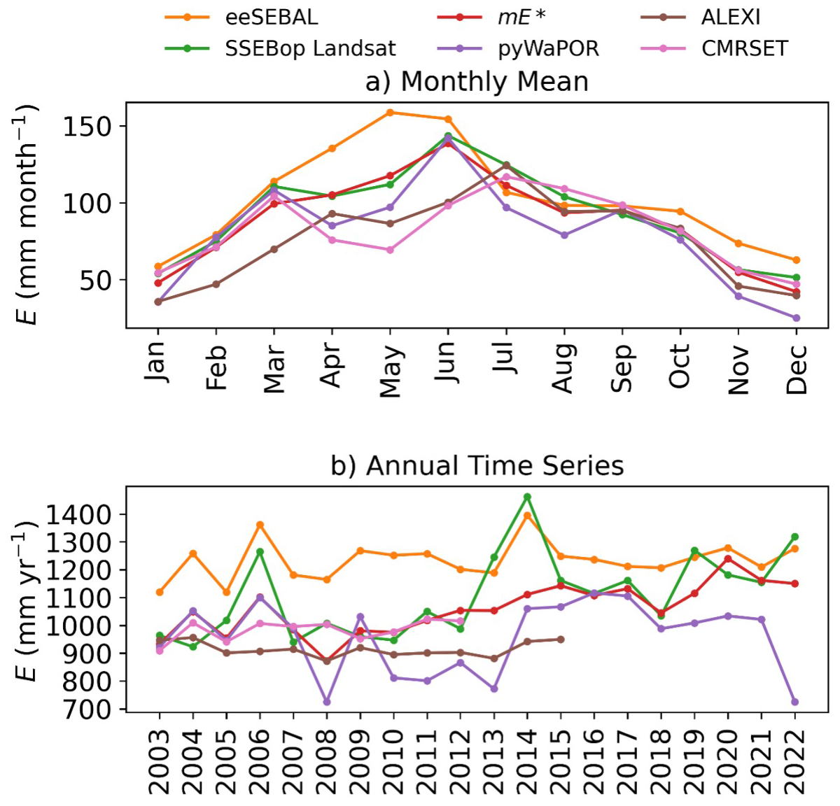
Figure C2 Comparison of the posterior mean ($m_E^{*}$) to the prior data sets describing the evaporation (E) variable in the Hindon basin, the top panel depicts (a) monthly mean E, and the bottom panel (b) shows the annual E time series.

C2 Comparison of individual gridded products to the posterior means

This section presents the spatial maps of the deviation of the individual precipitation and evaporation products from their posterior mean.

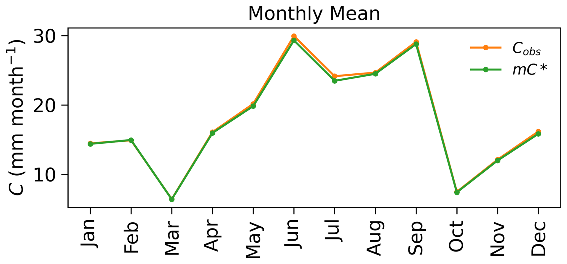
Figure C3 Comparison of the monthly mean posterior mean (mC*) to the prior data describing the surface water imports (C) variable in the Hindon basin.

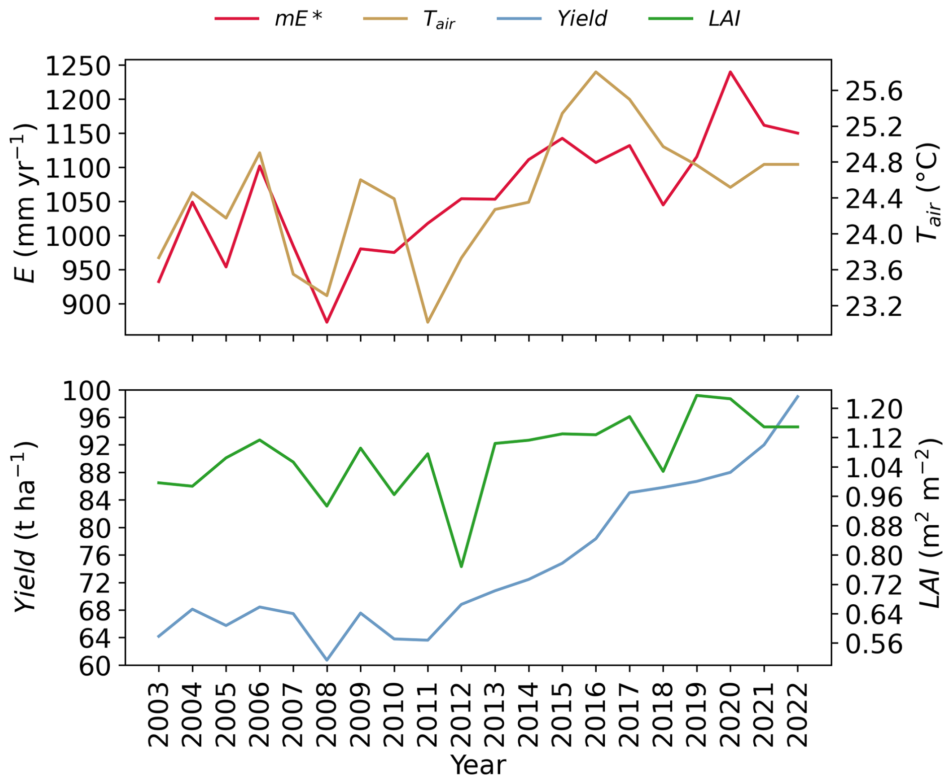
Figure C4 Interplay between the annual: evaporation posterior mean (${\mathrm{m}}_E^{\ast }$), air temperature variable from GLDAS Noah Land Surface Model v2.1 (Rodell et al., 2004), MODIS 15 Leaf Area Index (LAI) (Myneni et al., 2021), and district-wise sugarcane crop yield from International Crops Research Institute (2020) for the Semi-Arid Tropics database.

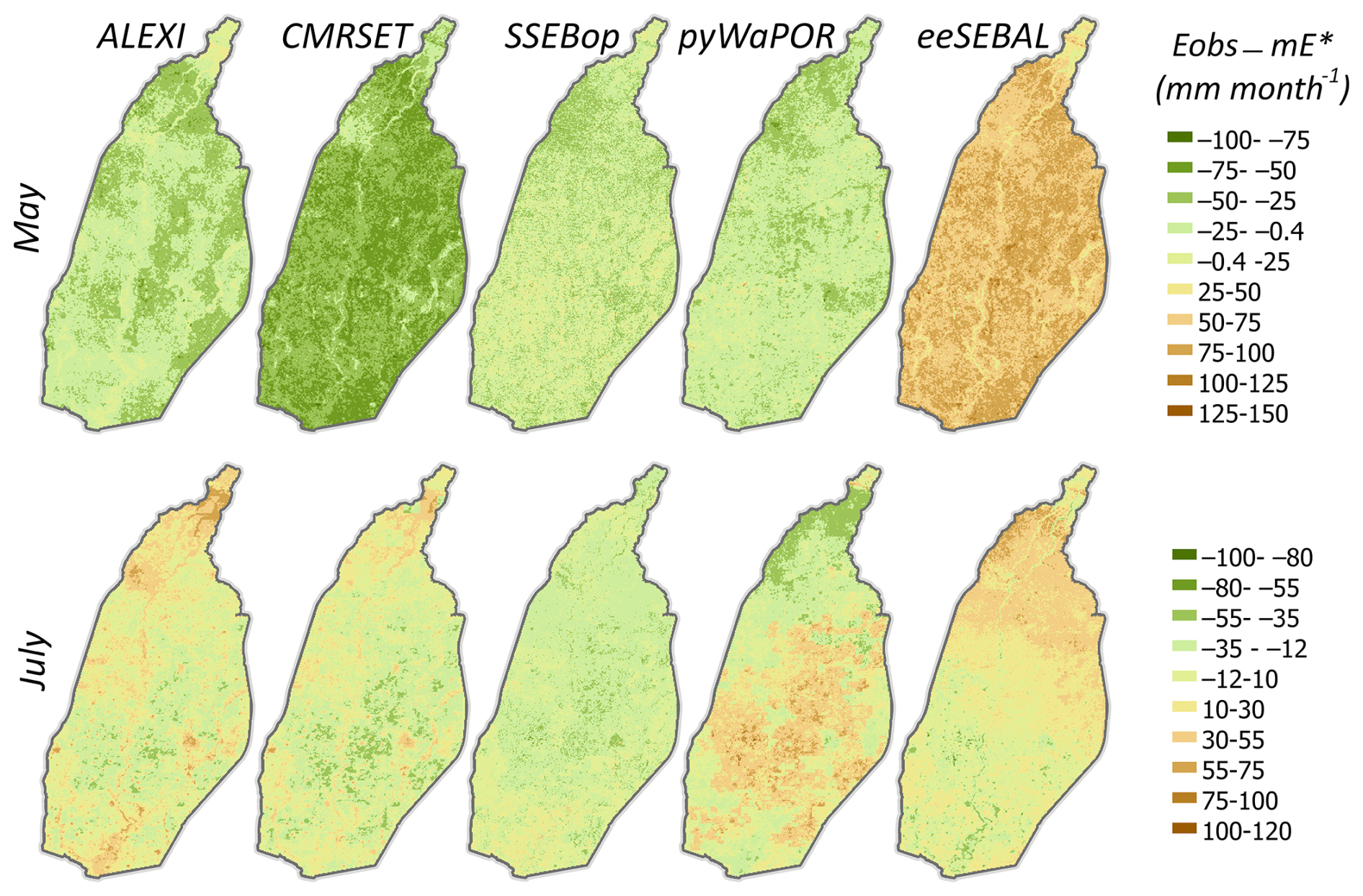
Figure C5 Spatial deviation of the evaporation (E) observations from the posterior mean (${\mathit{E}}_{\mathrm{obs}}-{\mathit{m}}_E^{\ast }$) for May and July of 2009.

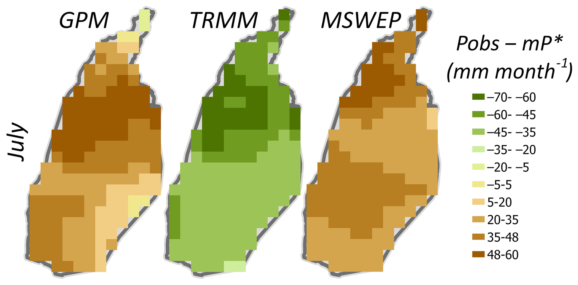
Figure C6 Spatial deviation of the precipitation (P) observations from the posterior mean (${\mathit{P}}_{\mathrm{obs}}-{\mathit{m}}_P^{\ast }$) for May and July of 2009.

C3 The sensitivity of the posterior results to the GRACE input data

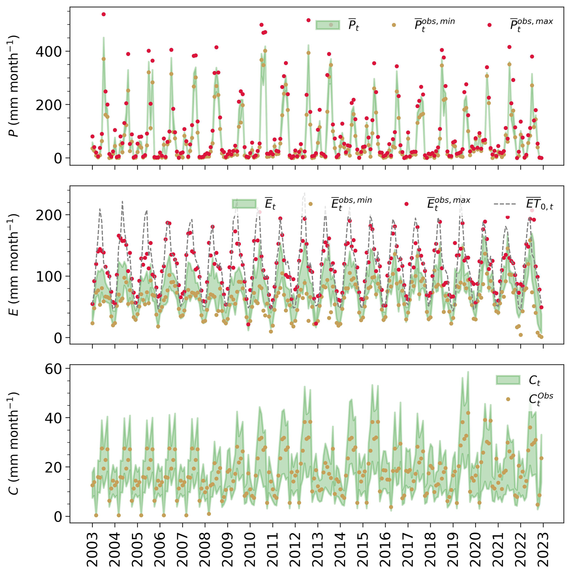
Figure C7 Posterior and prior water balance plots correspond to the case using the GRACE CSR spherical harmonic (SH) solution as an input to the probabilistic water balance model.