Year-round measurements of evaporation from northern latitude wetlands in Norway

As the atmosphere warms, atmospheric evaporative demand is expected to increase across many high-latitude ecosystems, while the duration of seasonal snow cover is projected to change. In Norway, a typically moisture-rich region, improved understanding of the controls on evaporation is needed to assess how these changes may affect ecosystem hydrology. In this study, we used year-round evaporation estimates from four eddy-covariance wetland sites in Norway to quantify evaporation and identify its main controls. To estimate monthly, seasonal, and annual evaporation, eddy-covariance data were gap-filled using a random forest model. The sites cover a latitudinal gradient from 60 to 78° N, a precipitation gradient from 218 to 968 mm per year and a gradient in mean temperature from −3.9 to 2.7 °C. To identify evaporation controls, we performed a factor analysis on observed time series in the snow-free and snow-covered season, separately. In addition, we compared the observed evaporation with the results of a Penman-Monteith model. We found that ecosystem evaporation was mainly controlled by atmospheric evaporative demand, both in the snow-free and the snow-covered season, whereas soil moisture likely never decreased to a level where it restricted evaporation. However, the sensitivity of the Bowen ratio to the vapour pressure deficit varied between sites, showing a decrease in the Bowen ratio beyond a vapour pressure deficit of 1 kPa at sites with a larger cover of open water and non-vascular vegetation compared to a site with a higher cover of vascular plants. Annual evaporation ranged from 80 to 208 mm, equivalent to 9 % to 30 % of the total precipitation. In the warm season, evaporation was typically around 50 % of the seasonal precipitation, reaching a maximum of 72 %. Sites and years with long-duration snow-cover had lower annual evaporation. Compared to other northern latitude sites in the FLUXNET2015 data set, evaporation was lower than expected from the mean temperature of the warm season. Our results show that evaporation is an important part of the northern latitude water balance, especially during the warm season and in regions with low precipitation. Furthermore, our results indicate that earlier snow-cover melt-out and increased vapour pressure deficit have the potential to increase annual evaporation.

1 Introduction

There is a high demand for observations of evaporation in fast-warming northern latitude regions, which are characterised by a seasonal snow cover. Norway is situated in a typically moisture rich region with numerous lakes and wetlands. Wetlands cover about 8.9 % of the area in Norway (Bryn et al., 2018), and provide important ecosystem services such as carbon storage and biodiversity. Northern wetlands constitute a large carbon storage, and have acted as a carbon sink during the Holocene, however there is uncertainty related to the future carbon accumulation and decay (e.g., Charman et al., 2013; Bacon et al., 2017). Adequate moisture availability is crucial for wetland functioning, and assessment of wetland water fluxes is vital to understand the wetland-climate feedbacks (Waddington et al., 2015).

In northern latitude regions, evaporation is often energy-limited (McVicar et al., 2012), although it can be water-limited in drier areas, such as in parts of central-western (Wang et al., 2013) and north-western Canada (Spence and Rouse, 2002). Evaporation is traditionally considered a minor component of the annual water balance in Norway (Erlandsen et al., 2021). However, it is expected that the atmospheric demand for water will increase as vapour pressure deficit increases (Masson-Delmotte et al., 2018; Grossiord et al., 2020) and snow cover duration declines in many areas (Rizzi et al., 2017; Mohammadzadeh Khani et al., 2022). The term “atmospheric evaporative demand” is used to quantify the combined effect of the available energy for evaporation and the ability of the atmosphere to receive water vapour, and is typically used interchangeably with “potential evaporation” (Peng et al., 2018). The atmospheric demand typically increases with increasing net radiation, vapour pressure deficit and wind speed (e.g., Penman and Keen, 1948; Katul et al., 2012).

By increasing the evaporative demand, vapour pressure deficit influences the partitioning of available energy between sensible and latent heat fluxes (evaporation), a balance commonly expressed through the Bowen ratio, defined as the ratio of sensible to latent heat flux. Increased vapour pressure deficit enhances the evaporative demand and tends to lower the Bowen ratio when water is available, whereas water-limited conditions can increase the Bowen ratio. Liljedahl et al. (2011) found that the Bowen ratio remained below 1 for vapour pressure deficit exceeding 0.3 kPa in wet soils of two drained thaw-lake basins on the Arctic Coastal Plain of Alaska, whereas drier soils showed higher Bowen ratios under comparable vapour pressure deficit. Westermann et al. (2009) found higher rates of Bowen ratio with lower soil water content in a high-arctic permafrost site on Svalbard. Further, the surface ability to transport water can influence the relation of vapour pressure deficit and Bowen ratio (Helbig et al., 2020).

Snow cover influences evaporative demand by reducing net radiation through its high albedo compared to snow-free surfaces, and by diverting available energy toward snowmelt rather than surface heating. Pirk et al. (2023) found that annual total evaporation from an alpine tundra site decreased by 50 % in a year with a delayed snow-cover melt-out date of one-month.

To better understand how northern latitude ecosystems may respond to a future longer snow-free season and increased evaporative demand, we need more knowledge on the magnitude and controls of evaporation in these ecosystems. Observations of evaporation are vital, both to increase process understanding and to constrain models. Existing hydrological models show large spread in evaporation estimates, ranging from 178 to 500 mm annually for mainland Norway (Erlandsen et al., 2021). Routine observations of evaporation in Norway are lacking, and only a few experimental eddy-covariance sites are currently in place. Although evaporation data from eddy-covariance measurements are available in the wider northern latitude region through networks such as FLUXNET (Pastorello et al., 2020), previous studies have often focused on forested areas, including sites in Finland and Sweden. Due to the large climatic gradients ranging from moist and mild climate in the coastal west to dry and cold climate in the continental east, it is uncertain if existing observations are representative of ecosystems in the larger region. In addition, emphasis has been on carbon fluxes rather than water fluxes (Baldocchi, 2020). Apart from forest, land cover types such as wetland and tundra are widespread in the region, and our knowledge on the magnitude and dynamics of evaporation in these ecosystems is highly uncertain.

This study explores how evaporation and its main environmental controls vary with climatic gradients of temperature and precipitation at northern high latitude sites. We use new observations from three wetland and tundra sites in mainland Norway, a previously poorly represented region (Pallandt et al., 2022). We also include a site on Svalbard to cover a larger climatic gradient. We aim to quantify evaporation at sub-daily to annual time scales. Furthermore, we explore to what extent available energy controls evaporation, and what the role of other factors, such as vapour pressure deficit, soil moisture and snow cover, play in controlling evaporation rates. Our main objective is to quantify evaporation from northern latitude wetlands in Norway and identify its main climatic controls. More specifically, we look at (1) controls on evaporation at an hourly timescale, (2) magnitude and seasonality of daily and monthly evaporation rates and (3) annual evaporation and interannual variability across climatic gradients. To place the new sites in a regional context, we compare the annual evaporation of our sites to that of existing northern latitude sites in the FLUXNET2015-dataset.

2 Materials and Methods

2.1 Study sites

The four study sites are Hisåsen, Finse and Iškoras on mainland Norway and Adventdalen on Svalbard. The sites are located along gradients in latitude, temperature and precipitation, covering a latitudinal gradient from 60–78° N, a precipitation gradient from 218–968 mm per year and a gradient in mean temperature from -3.9–2.7 °C (see Fig. 1 and Table 1). Compared to northern latitude (above 60° N) sites available in the FLUXNET2015 dataset (Pastorello et al., 2020), our study sites span approximately the full range of latitudes and annual precipitation rates (including one site with higher precipitation), whereas they are somewhat in the mid-range with respect to mean annual temperature (Fig. 1b). The ecosystem types at the three mainland sites have been classified according to the “Nature in Norway” ecosystem and landscape diversity framework (Halvorsen et al., 2020). Photos of the study sites are available in Fig. 2.

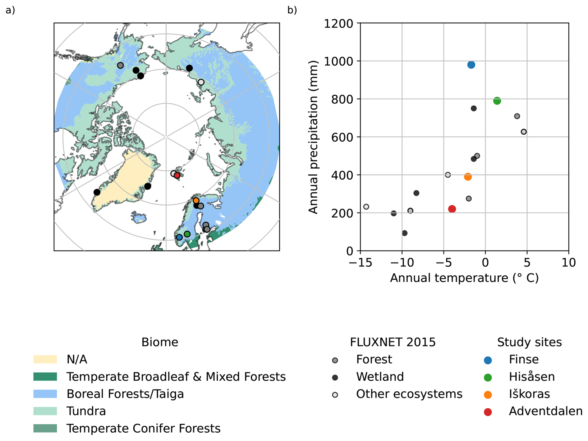
Figure 1 Location (a) and climatic context (b) of the four sites included in the study compared to selected northern latitude sites from FLUXNET2015 (Pastorello et al., 2020). Finse in blue, Hisåsen in green, Iškoras in orange, Adventdalen in red and FLUXNET sites in greyscale. The symbols of the FLUXNET sites indicates if the site is a wetland (black), evergreen need leaf forest (dark grey) or other ecosystem types (light grey). The latter category includes one site in each of the following ecosystem types: open shrubland, cropland, grassland, and snow/ice. Only FLUXNET sites located above 60 °N latitude and with Creative Commons (CC-BY-4.0) licence were included in the comparison (see a list of the included sites in Table E1). The biome map in panel (a) is from Dinerstein et al. (2017).

Table 1 Site information, mean annual precipitation (MAP), and mean annual air temperature (MAAT) for the climate reference period 1991–2020 (based on data from The Norwegian Meteorological Institute).

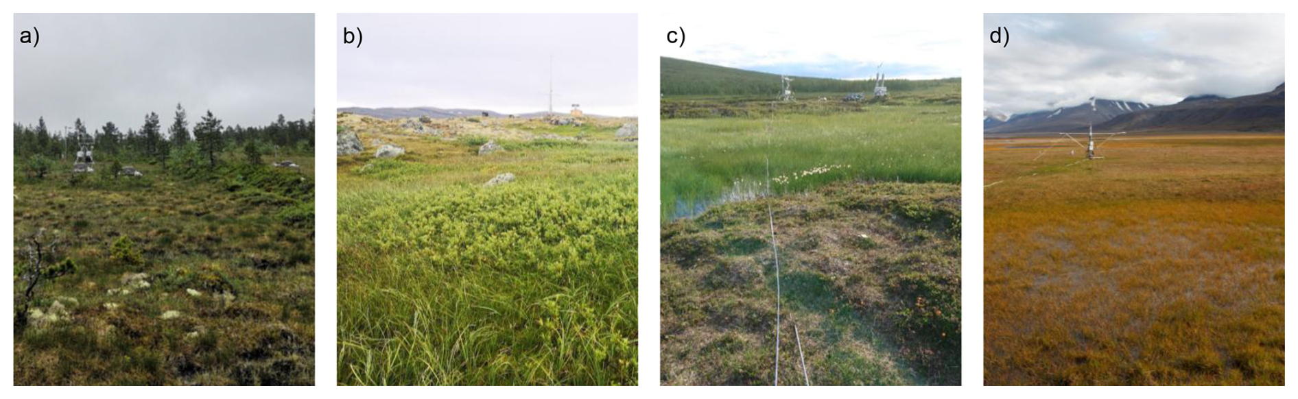
Figure 2 Photos from (a) Hisåsen 21 June 2021, (b) Finse 9 September 2020, (c) Iškoras 27 July 2020 and (d) Adventdalen 19 August 2013.

The Hisåsen site is a boreal peatland site, located south of the hill Hisåsen in the Regnåsen-Hisåsen nature reserve in eastern Norway. The area is undulating, slightly sloping towards north and covered by forest and peatlands. The climate is continental subarctic (Dfc), according to Köppen's classification, with a mean annual temperature of 2.7 °C and a mean annual precipitation of 857 mm. The measurement tower is located on a drained peatland with organic soils surrounded by forest on glacial till (NGU, 2023). The footprint ecosystem types are predominantly strongly lime-poor fen and lime-poor drained fen, according to the Nature in Norway system (maps are publicly available at http://github.com/geco-nhm/NiN_Hisaasen, last access: 28 November 2023). The vegetation is low and dominated by sedges, mosses and shrubs, such as Salix herbacea and Empetrum nigrum. A few trees, such as Pinus sylvestris and Betula pubescens are present.

Finse is a sub-alpine tundra and wetland site, located in the valley Finsedalen north of the Hardangerjøkulen glacier. The valley runs towards east-southeast, and wind directions at the site are controlled by the valley. The climate is tundra (ET), with mean annual temperature of −1.1 °C and mean annual precipitation of 967 mm. The climate has an oceanic influence, located approximately 140 km from the coastline in the west and exposed to the mild and moisture-baring westerlies. The instrument tower sits on a ridge running southwest-northeast. Southeast, the ridge slopes down towards the river Ustekveikja draining the lake Finsevatnet, located approximately 1 km east of the tower. The footprint ecosystem types are predominantly lime-poor open fens, arctic-alpine heath and lee side as well as snowbeds (Bryn, 2020; Halvorsen et al., 2020). The soil is thin and consisting of discontinuous glacial till with thickness less than 0.5 m and glacifluvial deposits (NGU, 2023). The vegetation is dominated by shrubs, such as Salix herbacea and Empetrum nigrum, and mosses and lichens in the drier areas and sedges and mosses in wetter areas.

Iškoras is a palsa mire site located north of the mountain Iškoras in the plateau area of Finnmarksvidda in northern Norway. The climate is continental subarctic (Dfc), with a mean annual temperature of −1.4 °C and a mean annual precipitation of 417 mm. The tower is located on a peat plateau surrounded by mires and ponds (Martin et al., 2019), with partly organic soil and partly glacial till (NGU, 2023). Shrubs and lichens dominate dry, elevated palsas, whereas sedges and mosses dominate wetter areas near unvegetated ponds (Pirk et al., 2024). The shrubs are species such as Betula nana and Empetrum nigrum. Bog and open fen are the dominating ecosystem types (Halvorsen et al., 2020; Anders Bryn, personal communication, 2023). The peat plateau lies north of the mountain range Iškoras, and the terrain slopes gently towards north.

Adventdalen (NO-Adv) is an Arctic site featuring polygonal tundra, located in the valley Adventdalen on Spitsbergen, Svalbard. The climate is tundra (ET), with a mean annual temperature of −3.9 °C and a mean annual precipitation of 218 mm. The climate has an oceanic influence, located approximately 6 km from the coast. The tower is located on a river terrace on the flat part of a large alluvial fan, and the soil consists of a few decimetres of fine-grained eolian deposits on top of coarser-grained alluvial deposits (Pirk, 2017). The vegetation is very low, dominated by dwarf shrubs like Salix polaris at dry places and mosses and sedges in wet depressions (Pirk et al., 2017).

For each site, the 3–4 years with the most complete data collection was chosen as the site measurement period. Thus, the measurement period varies slightly between sites (Table 1). Figure 3 shows monthly mean temperature and cumulative precipitation at the nearest climate station of The Norwegian Meteorological Institute (MET Norway) for the reference period (1990–2020) and for each year in the respective measurement periods. Precipitation is relatively evenly distributed over the year at all sites, with the wettest month having a mean precipitation of 2.7 to 3.6 times the precipitation of the driest month. The wettest month at each site occurs in summer or early autumn (July at Iškoras, August at Hisåsen and September at Finse and Adventdalen). The driest month occurs in spring or early summer (March at Hisåsen and Iškoras, April at Finse and May at Adventdalen). Monthly mean temperature typically peaks in July and is below zero from November–March at Hisåsen, October–April at Finse and Iškoras and October–May at Adventdalen.

Overall, the measurement years were warmer than the reference period at all sites (Fig. 3). At Hisåsen, the annual mean temperature was warmer than normal for all years (0.1–0.2 °C), with 2020 being the warmest year. Annual precipitation was both lower and higher than normal (ranging from 88 %–115 % of the long term mean) with 2020 being the wettest year. A similar pattern was found at Finse, with all years being warmer than normal (0.1–1.0 °C), and annual precipitation both higher and lower than normal (ranging from 78 %–133 % of the long term mean), with 2020 being the wettest year. Iškoras was the only site where annual temperature was both higher and lower than normal (varying from 0.4 °C lower in 2019 and 2021, to 0.7 °C higher in 2020). However, all years had temperatures 0.2–4.6 °C above normal in the warm season (May–September). Annual precipitation ranged from 101 %–118 % of the long term mean, with 2019 and 2020 being the wettest years. At Adventdalen, all years were warmer (0.4–3.8 °C) and wetter (114 %–143 %), than the long term mean, with 2016 being the warmest and wettest year as well as the warmest ever recorded at the station. Annual precipitation ranged from 114 % of the long term mean in 2013 to 143 % in 2016. The temperature deviations were typically larger in autumn and winter (September–March) than in spring and summer (April–August). On average, 40 %–44 % of the yearly precipitation fell as snow at Finse, Iškoras and Adventdalen, while 11 % fell as sleet and 45 %–48 % fell as snow. At Hisåsen, the distribution was 20 % snow, 13 % sleet and 67 % rain (Table B1).

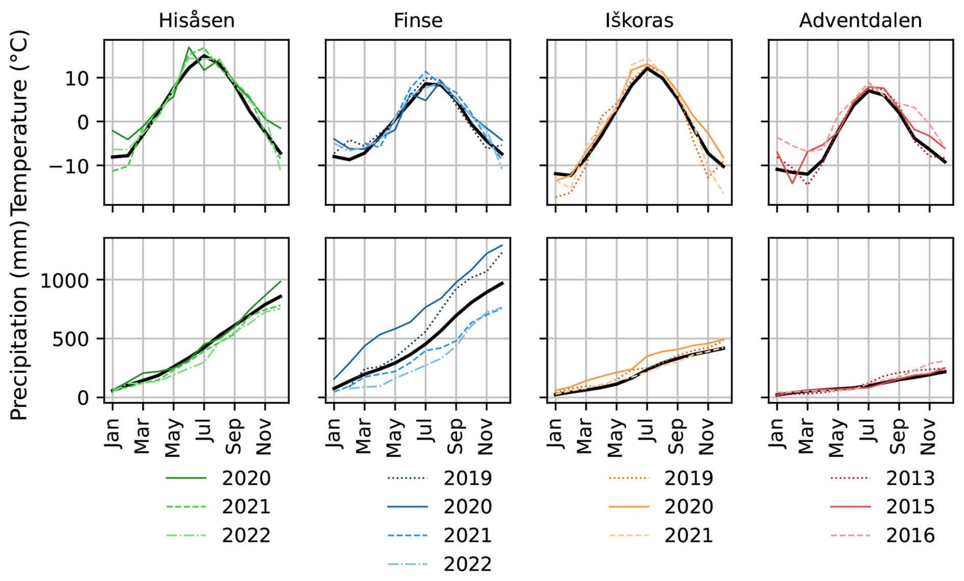
Figure 3 Monthly mean temperature (upper row) and cumulative precipitation (lower row) in climate reference period (black lines) and measurement periods (coloured lines) at each site's nearest MET Norway weather station.

2.2 Data sources and processing

2.2.1 Eddy covariance data

To measure ecosystem evaporation, we used the eddy covariance method (e.g., Burba, 2022). At all sites, we measured water vapour mixing ratio using an enclosed gas analyser (Li-Cor LI7200). Three-dimensional wind speed measurements were made by sonic anemometer (Campbell Sci. CSAT3 at Finse and Iškoras, Gill HS-50 at Hisåsen, and a Metek USA-1 at Adventdalen). We processed the raw eddy covariance data in the software EddyPro version 6.2.0, using a double rotation tilt correction of the anemometer, block average method to extract turbulent fluctuations and constant time lag between wind and gas concentration based on pump flow rate. We applied spectral corrections in the high frequency range according to Moncrieff et al. (1997), and in the low frequency range according to Moncrieff et al. (2005). The resulting time series of half-hourly evaporation flux was filtered according to the 0–2 flagging scheme based on tests proposed in Foken and Wichura (1996), discarding all observations with quality flags >0. Additionally, the time series of fluxes and ancillary variables measured by the eddy covariance system (friction velocity and wind speed) were filtered based on a statistical screening of the raw data, using tests from Vickers and Mahrt (1997) with the default test thresholds in Eddypro 6.2.0 (hard-flags only).

To estimate daily, monthly and annual evaporation, we filled the gaps in evaporation time series by building a random forest regression model (Python package Sklearn) for each site, using gap-filled ancillary data as predictors (Tables 2 and 4). The observed evaporation was averaged to hourly mean values. Before building the regression, the dataset was split into 75 % training and 25 % test data. The root-mean-square error (RSME) of test data predictions varied from 0.011 to 0.015 mm h⁻¹. A time series plot of observed and gap-filled evaporation is available in Fig. C1, and the percentage of gap-filled and observed data for each site and each month is available in Table C1.

Due to the large variation in surface cover in the footprint area of the Finse site, we grouped the data based on the dominating wind direction (east and west) and gap-filled the two wind direction sectors separately (as done in Pirk et al., 2023). Only data from the western sector were included in this study, as the western surface cover is more comparable to the other sites in the study.

2.2.2 Measured ancillary local data

We used locally measured meteorological and surface variables to gap-fill the evaporation time series and to identify controls on evaporation on a sub-daily timescale (hourly values). At each site, measurements of local meteorological and surface variables (Table 2) were sampled with 1 min time resolution. We discarded periods of data with sensor error through visual inspection. After filtering, the values were aggregated to hourly means. Gaps in the time series of meteorological variables (air temperature, vapour pressure deficit, wind speed, incoming radiation and atmospheric pressure) were filled using the bias-corrected corresponding ERA5 Land variable (Muñoz Sabater, 2019), downloaded from the Climate Data Store (CDS, accessed on 22 February 2023) of the Copernicus Climate Change Service (C3S). We bias-corrected the ERA5 Land variables by using a simple linear regression with the corresponding local variable, built by using either data from the whole year or, when data coverage for each season was sufficient, by building seasonal linear regressions for winter (December–February), spring (March–May), summer (June–August) and autumn (September–November) separately. Vapour pressure deficit was derived from relative humidity and temperature. We created a gap-free time series of hourly precipitation using data from the nearest MET station (Table A1), gap-filled with ERA5 Land precipitation. The hourly time series of precipitation was used to derive a new variable called “time since rain” (as described in Sect. 2.2.3), that we used as a proxy of soil moisture availability, in addition to point measurements of soil water content where available. The time since rain variable was considered to be more representative of a larger area than point measurements. To calculate monthly and annual evaporation ratio (evaporation as fraction of precipitation) we used monthly and annual precipitation from nearest MET Norway station (Table A1).

Table 2 Measured ancillary data.

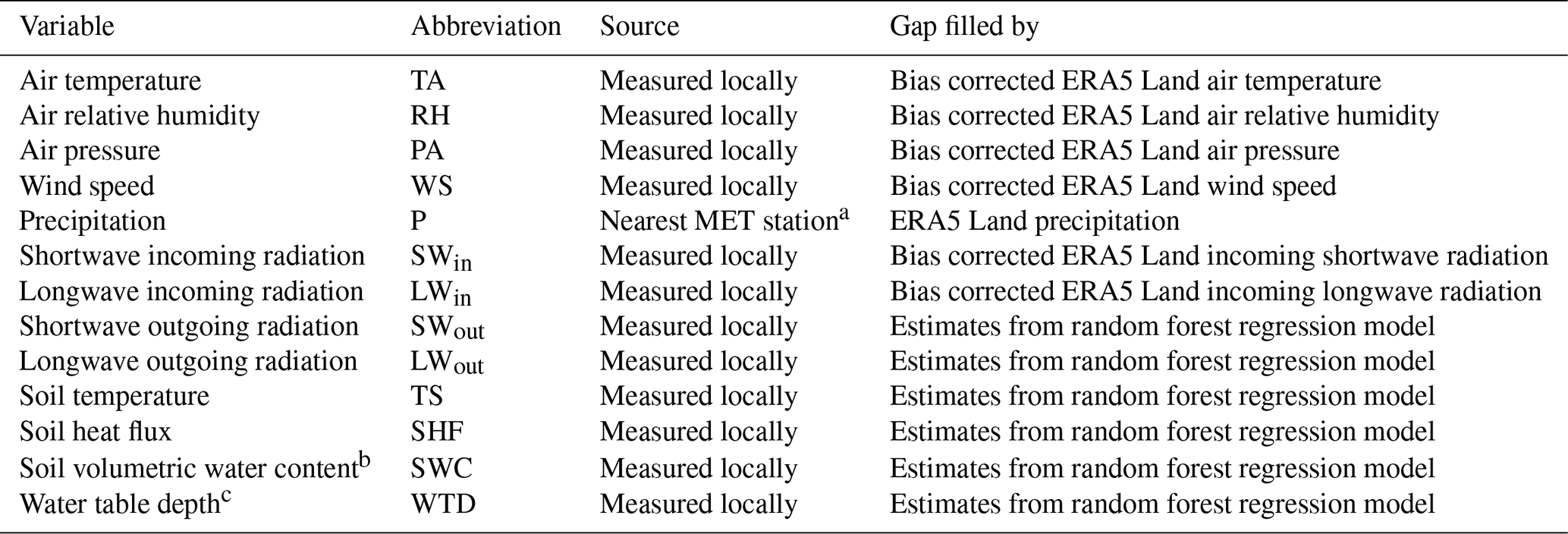
^a At sites Hisåsen and Iškoras, precipitation is measured locally in the snow-free season and from the nearest MET Norway station in the snow-covered season. ^b Not measured at Adventdalen. ^c Only measured at Hisåsen.

The soil heat flux (SHF in Eq. 3), was estimated using measurements from soil heat flux plates (Hukseflux), available at each site. Further details about measured ancillary local data can be found in Bekken et al. (2025) (Hisåsen), Pirk et al. (2023) (Finse), Pirk et al. (2024) (Iškoras) and Pirk et al. (2017) (Adventdalen). The measurements of net shortwave and long wave radiation, soil heat flux and sensible and latent heat from the eddy covariance measurements were used to calculate the degree of energy balance closure at each site (Table 3). The degree of energy balance closure was estimated from the slope of the linear regression of the sum of latent and sensible heat against available energy (difference between net radiation and soil heat flux). Energy balance closure was calculated both for observations in the snow-free season only and for the full year (Figs. F1 and F2).

Table 3 Energy balance closure at each site for observations in the snow-free season only (first row) and for the full year (second row) See also Figs. F1 and F2.

We gap-filled ancillary surface variables (outgoing radiation, soil temperature, soil water content and soil heat flux) by using predictions from a random forest regression (Python package Sklearn). A random forest regression was built for each variable, using gap-filled meteorological variables and derived variables (Table 4) time since rain, growing degree days and snow cover as predictors.

2.2.3 Derived ancillary data

To provide additional information for the gap-filling of surface variables and evaporation fluxes, we derived variables representing snow cover, soil moisture availability (time since rain) and phenology (growing degree days). Time since rain was calculated from the gap-filled time series of hourly precipitation. If hourly precipitation exceeded 0.1 mm, we defined it as a rain event. For each time step, we then calculated hours passed since the last rain event. In the snow-covered season, we set time since rain to zero. To calculate growing degree day, we used the gap-filled time series of hourly temperature. For each year, growing degree day was then calculated as

$$\begin{array}{}\text{(1)}& {\text{GDD}}_i=\sum _{n=\mathrm{1}}^{i}max\left({\displaystyle \frac{T_{\max }\left(d^{\prime }\right)+T_{\min }\left(d^{\prime }\right)}{\mathrm{2}}},\mathrm{0}\right)\end{array}$$

where T_max and T_min are daily maximum and minimum temperatures of day i, respectively.

The ground surrounding the towers, approximately 1 km², was classified as either (i) snow-free, (ii) partly snow-covered or (iii) fully snow-covered, by visually inspecting satellite images (Sentinel-2, natural colour, accessed through Copernicus Browser; Copernicus Data Space Ecosystem, 2024) during spring and autumn each year for each station. The start/end of the snow-free season was set to the date of the first/last available image of snow-free ground. Similarly, the start/end of the snow-covered season was set to the date of the first/last image with a full snow cover that lasted through the winter. The period in between was considered as a shoulder season, with either partly snow-covered ground or a snow cover lasting only for a short while. Controls in the snow-free season were analysed by masking data from days when the ground was either fully or partly snow-covered.

Table 4 Derived ancillary data.

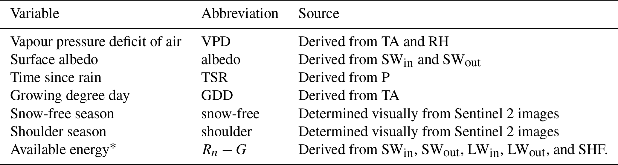
^∗ Used as forcing for Penman-Monteith equation (described in Sect. 2.3.2). Not included in gap-filling or factor analysis.

2.3 Identifying controls on evaporation

To study the controls on evaporation on a sub-daily timescale, we used hourly observations of evaporation from the eddy covariance data. Only observed data were used in this part of the study (i.e. gap-filled values were not included). We first calculated Pearson correlation coefficients between hourly evaporation and local meteorological and surface variables for the snow-free and snow-covered season separately, and tested whether the correlation coefficients were significant at significance levels p<0.05, p<0.01 and p<0.001. Available energy (R_n−G) is included in the analysis of correlations as it is a forcing variable in the Penman-Monteith equation (described in Sect. 2.3.2), but is not included as a predictor variable in the gap-filling regression model or included in the factor analysis. To avoid spurious predictor importances due to the large degree of covariance between the controls of evaporation, we performed a Factor analysis (similar to the analysis in Thunberg et al. (2021b) and Thunberg et al. (2021a)) to group variables with a large degree of common variance. To evaluate how the partitioning between sensible and latent heat flux changed with atmospheric and surface controls, we calculated mean Bowen ratio, i.e. the ratio of sensible to latent heat flux, for bins of vapour pressure deficit and soil water content. Finally, we modelled hourly evaporation using the Penman-Monteith equation to test how a widely used model is able to capture the sensitivity of evaporation to climatic and surface controls. We focus on controls in the snow-free season, as 68 % to 86 % of the annual evaporation occurred in the snow-free season.

2.3.1 Factor analysis

To group variables with common variability pattern, and identify control variables with a high degree of common variance as evaporation, we performed an exploratory factor analysis using the Python package “Factor Analyzer”. The factor analysis groups the observed variables into underlying unobserved variables called factors. Each factor explains a certain variance in the dataset of observed variables, with the first factor explaining the most. The result of the analysis can be interpreted by the observed variable's factor loading, i.e. the correlation coefficient between a factor and an observed variable. Observed variables with a high degree of common variance will load high on the same factor. For each site and each season (snow-free and snow-covered), we first evaluated the suitability of the dataset for factor analysis using the Kaiser-Meyer-Olkin (KMO) criterion (Cureton and D'Agostino, 2013). To exclude data unacceptable for factor analysis, the analysis was performed only if the dataset KMO-value exceeded 0.5 (Kaiser and Rice, 1974). Most sites and seasons had KMO-values >0.7 (Table D1). The number of factors was based on the Kaiser criterion, with an eigenvalue of 1 as threshold. For the final factor extraction, we used “Varimax” orthogonal rotation, which seeks to minimize the number of variables that have high loading on each factor. We specifically looked at variables with a high degree of loading on the same factor as evaporation.

2.3.2 Penman-Monteith Estimates

Hourly evaporation in the snow-free season was modelled from the Penman-Monteith equation (Monteith, 1965) as:

$$\begin{array}{}\text{(2)}& E_{\mathrm{pm}}=\left({\displaystyle \frac{\mathrm{3.6}\times {\mathrm{10}}^{\mathrm{6}}}{{\mathit{\rho }}_{\mathrm{w}}{\mathit{\lambda }}_{\mathrm{v}}}}\right){\displaystyle \frac{\mathit{\delta }(R_n-G)+{\mathit{\rho }}_{\mathrm{a}}{c}_p{g}_{\mathrm{a}}\text{VPD}}{\mathit{\delta }+\mathit{\gamma }\left(\mathrm{1}+\frac{g_{\mathrm{a}}}{g_{\mathrm{s}}}\right)}}\end{array}$$

where E is evaporation rate in mm h⁻¹, ρ_w is the mass density of water in kg m⁻³, λ_v is the latent heat of vaporisation in J kg⁻¹, R_n−G is available energy in W m⁻², γ is the psychrometric constant in Pa °C⁻¹, δ is the slope of the saturation vapour pressure versus temperature curve in Pa °C⁻¹, ρ_a is the mass density of dry air in kg m⁻³, c_a is the specific heat of air in J °C⁻¹, VPD is air vapour pressure deficit in Pa, g_s is surface conductance and g_a is aerodynamic conductance, the latter two in m s⁻¹.

As forcing for the Penman-Monteith equation, we used the gap-filled ancillary data (Table 2). Available energy was estimated as the difference between net radiation and the soil heat flux, i.e. as:

$$\begin{array}{}\text{(3)}& R_n-G={\mathrm{SW}}_{\mathrm{in}}-{\mathrm{SW}}_{\mathrm{out}}+{\mathrm{LW}}_{\mathrm{in}}-{\mathrm{LW}}_{\mathrm{out}}-\mathrm{SHF}\end{array}$$

Aerodynamic conductance was estimated from average wind speed, WS, in m s⁻¹:

$$\begin{array}{}\text{(4)}& g_{\mathrm{a}}={\displaystyle \frac{\text{WS}}{{\left(\mathrm{6.25}\log \frac{z}{z_{\mathrm{0}}}\right)}^{\mathrm{2}}}}\end{array}$$

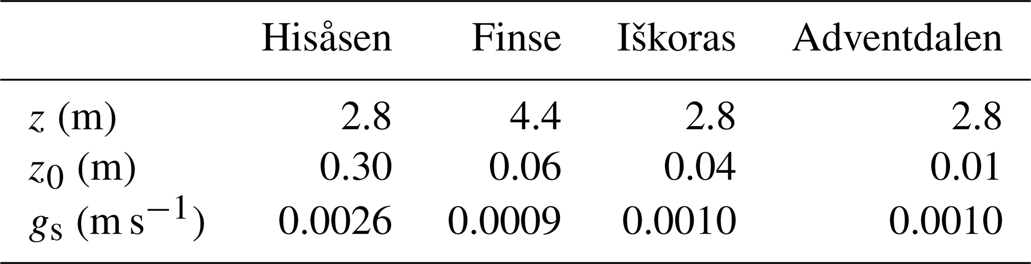
where z is wind speed measurement height and z₀ is the surface roughness length (estimated by visual inspection of vegetation height, see Table 5), both in m. We assumed the zero plane displacement to be zero, as the vegetation height is lower than 0.5 m at all sites (except for a few taller trees at Hisåsen). We used a site-specific constant surface conductance parameter g_s. An optimal g_s value for each site was derived by choosing the value that minimized the root square mean error (RMSE) in an interval of g_s from 0 to 0.05 m s⁻¹, covering the parameter range found for high latitude ecosystems in Kasurinen et al. (2014), with increments of 0.0001 m s⁻¹. Parameter values of z, z₀ and g_s at each site are listed in Table 5.

Table 5 Parameters used in the Penman-Monteith equation for estimating hourly evaporation.

To evaluate the sensitivity of the observed and estimated evaporation to various controls, we studied the relative error of the Penman-Monteith E_pm estimate to the observed evaporation E_obs. The relative error was calculated as $\frac{E_{\mathrm{pm}}-E_{\mathrm{obs}}}{\left|E_{\mathrm{obs}}\right|}$. We evaluated the sensitivity to the main forcing variables by looking for patterns in the mean relative error for bins of available energy and vapour pressure deficit. Furthermore, we evaluated the appropriateness of using a constant surface conductance parameter. The surface conductance parameter represents how available water is for evaporation on the surface, and can be seen as a combination of stomata conductance, leaf area index and soil water conductance. The surface conductance is typically modelled as a function of phenology, soil water content, solar radiation and temperature (e.g. Stewart, 1988). To evaluate the effect of soil moisture content and phenology on evaporation, we used a constant surface conductance and analysed the deviation from observed evaporation by looking at the tendency of the mean relative error to change for bins of the variables volumetric soil water content, time since rain and growing degree day. For volumetric soil water content, we used 20 bins in the range of observed values at each site, since the numeric value is not directly comparable between sites due to differences in soil properties. For time since rain and growing degree days, we used 24 h bins and 90 °C bins, respectively. For each bin, any data point where the relative error was more than 1.5 times the interquantile range below the first quantile or above the third quantile, was considered an outlier and removed. Only bins with a minimum of 10 data points remaining were used in analysis.

2.4 Regional comparison

To evaluate how the evaporation at the sites in this study compares to that of other northern latitude sites, we compared mean annual evaporation of the four sites to those in the FLUXNET2015 dataset (Pastorello et al., 2020). Only FLUXNET sites located above 60° N latitude with Creative Commons (CC-BY-4.0) licence were included in the comparison (see a list of the sites in Table E1). To test the annual evaporation dependency on the site mean temperature, we fitted a linear regression with annual evaporation as dependent variable and mean annual temperature as independent variable (including both our four study sites and the fourteen FLUXNET sites) and checked if the regression slope was significant at p<0.05. Furthermore, we tested if a better fit could be obtained by using warm season (May–September) mean temperature only instead of annual mean temperature.

3 Results

3.1 Controls on evaporation

Hourly evaporation was significantly correlated (p<0.001) with most of the climatic and surface controls, both in the snow-free and snow-covered season (Table 6), however, the relation was typically weak (r<0.5) except for a few controls related to atmospheric evaporative demand. In the snow-free season, evaporation had strong linear relations (r>0.7) to vapour pressure deficit and incoming shortwave radiation. Most stations had a strong or moderate relation (r>0.5) to air and soil temperature and outgoing longwave radiation, while the relation to other variables such as soil water content and wind speed was weak. In the snow-covered season, the correlation coefficients between evaporation and its controls were overall weaker than in the snow-free season, however the relation with incoming shortwave radiation and vapour pressure deficit was still strong or moderate (r>0.5) for all sites except at Adventdalen where only vapour pressure deficit had r>0.5 in the snow-covered season. For other controls, the relation to evaporation was weak (r<0.5).

Table 6 Pearson correlation coefficients between hourly evaporation (ET) and climatic and surface controls in both snow-free season and snow-covered season (see Tables 2 and 4 for abbreviations).

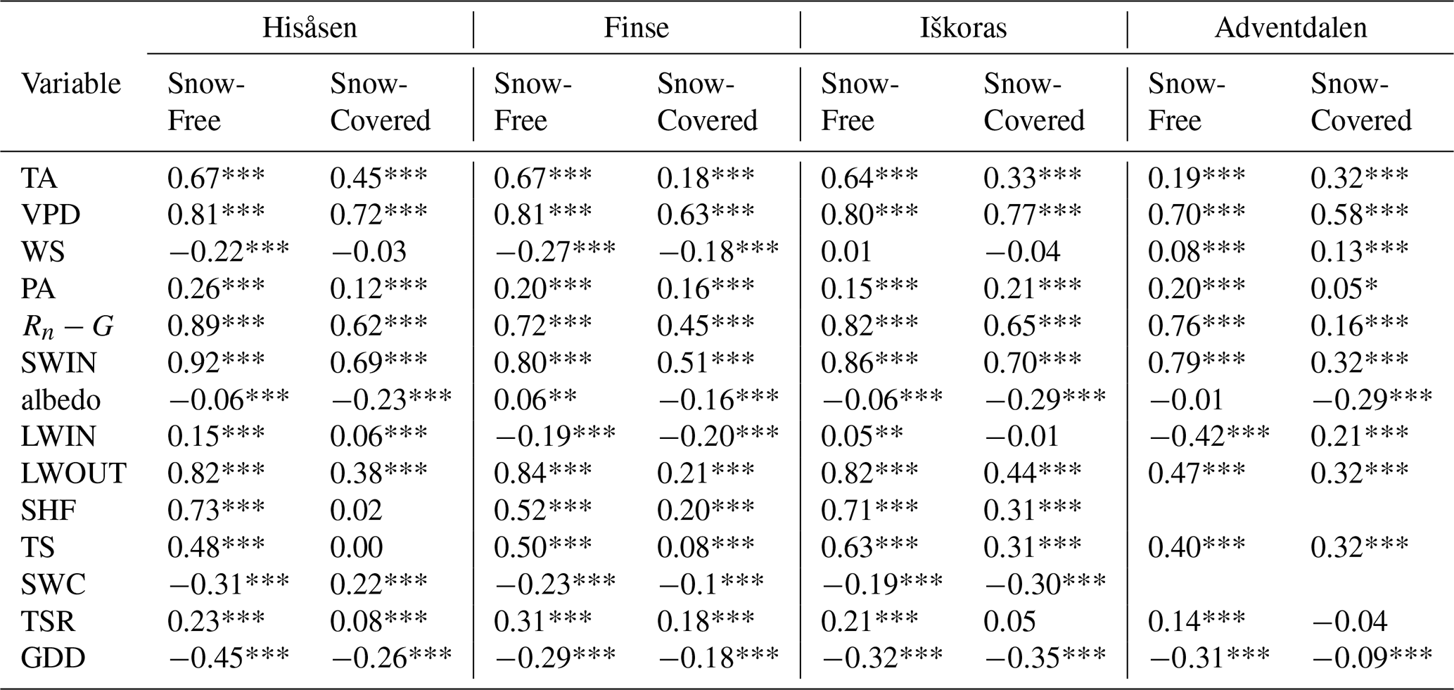
^* Significant at p<0.05. ${}^{**}$ Significant at p<0.01. ${}^{***}$ Significant at p<0.001.

The factor analysis showed that evaporation, vapour pressure deficit and incoming shortwave radiation had a high degree of shared variance both in the snow-free and snow-covered season. In the snow-free season, evaporation loaded highest on the first factor at Hisåsen, Finse and Iškoras (Fig. F3), together with vapour pressure deficit, incoming shortwave and outgoing longwave radiation (all with loadings >0.72). Air temperature, soil temperature and soil heat flux also loaded relatively high (>0.55) on the first factor. At Adventdalen, evaporation loaded highest on the second factor, together with incoming shortwave radiation and vapour pressure deficit (>0.62), whereas variables such as air temperature, surface temperature, and longwave outgoing radiation loaded high on the first factor. In the snow-covered season, evaporation had a lower loading on the first and second factor compared to the snow-free season, indicating a lower degree of common variance with other variables in the dataset (Fig. F4). At Finse and Adventdalen, the loading for evaporation was less than 0.51. At Hisåsen and Iškoras however, the evaporation loadings in the snow-covered season was more comparable to the snow-free season (>0.7). At Hisåsen, evaporation had a relatively high loading (0.76) on the first factor, together with shortwave incoming radiation (0.79) and vapour pressure deficit (0.90). At Iškoras, evaporation had a relatively high loading on the second factor (0.84) together with incoming shortwave radiation (0.76) and vapour pressure deficit (0.71).

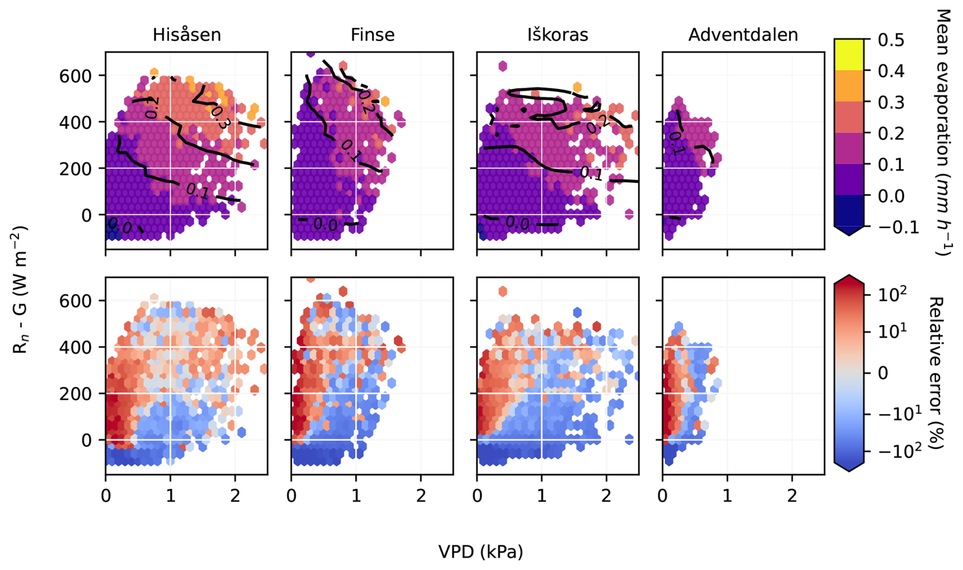
Figure 4 Upper row shows mean evaporation (mm h⁻¹) for bins of available energy (W m⁻²) and vapour pressure deficit (kPa) for observed evaporation in colour plot, and modelled evaporation in contour plot (solid black lines). The lower row shows the relative error (%) of the modelled evaporation by the Penman-Monteith equation for the same bins of available energy and vapour pressure deficit.

Comparing observed evaporation to Penman-Monteith estimates in the snow-free season, and looking at the distribution for bins of available energy and vapour pressure deficit (Fig. 4, upper row), we found that the Penman-Monteith equation reproduced the observed pattern of high evaporation when both vapour pressure deficit and available energy were high, and low evaporation when both controlling factors were low. The mean relative error (Fig. 4, lower row) showed a similar pattern across the sites, and showed a tendency towards overestimation (red hexagons) when vapour pressure deficit was low, and underestimation (blue hexagons) when high vapour pressure deficit was combined with low available energy. Furthermore, evaporation was underestimated by the Penman-Monteith equation when available energy was negative.

We evaluated the sensitivity of the observed and estimated evaporation, and the relative error of the estimates, to surface controls that can affect the surface water availability, such as the soil water content and time since rain (Figs. F5–F6), and growing degree day which is related to phenology (Fig. F7). Overall, the sensitivity of the Penman-Monteith estimates corresponded to the observed sensitivity, and there was no tendency for the relative error to increase or decrease with changes in the surface controls. However, there was a tendency towards higher relative errors at high values of soil water content at Finse (Fig. F5).

The Bowen ratio, i.e. the ratio of sensible to latent heat flux, decreased with vapour pressure deficit (Fig. F8), meaning that latent heat flux was increasingly favoured over sensible heat flux with increasing vapour pressure deficit. At vapour pressure deficit over 0.4 to 1.0 kPa, the Bowen ratio was under 1 and the latent heat flux dominated over sensible heat. At Hisåsen, the mean Bowen ratio stabilised at just below 1 for vapour pressure deficit exceeding 1.0 kPa, while at the other sites, it continued to decrease for the whole range of observed values of vapour pressure deficit.

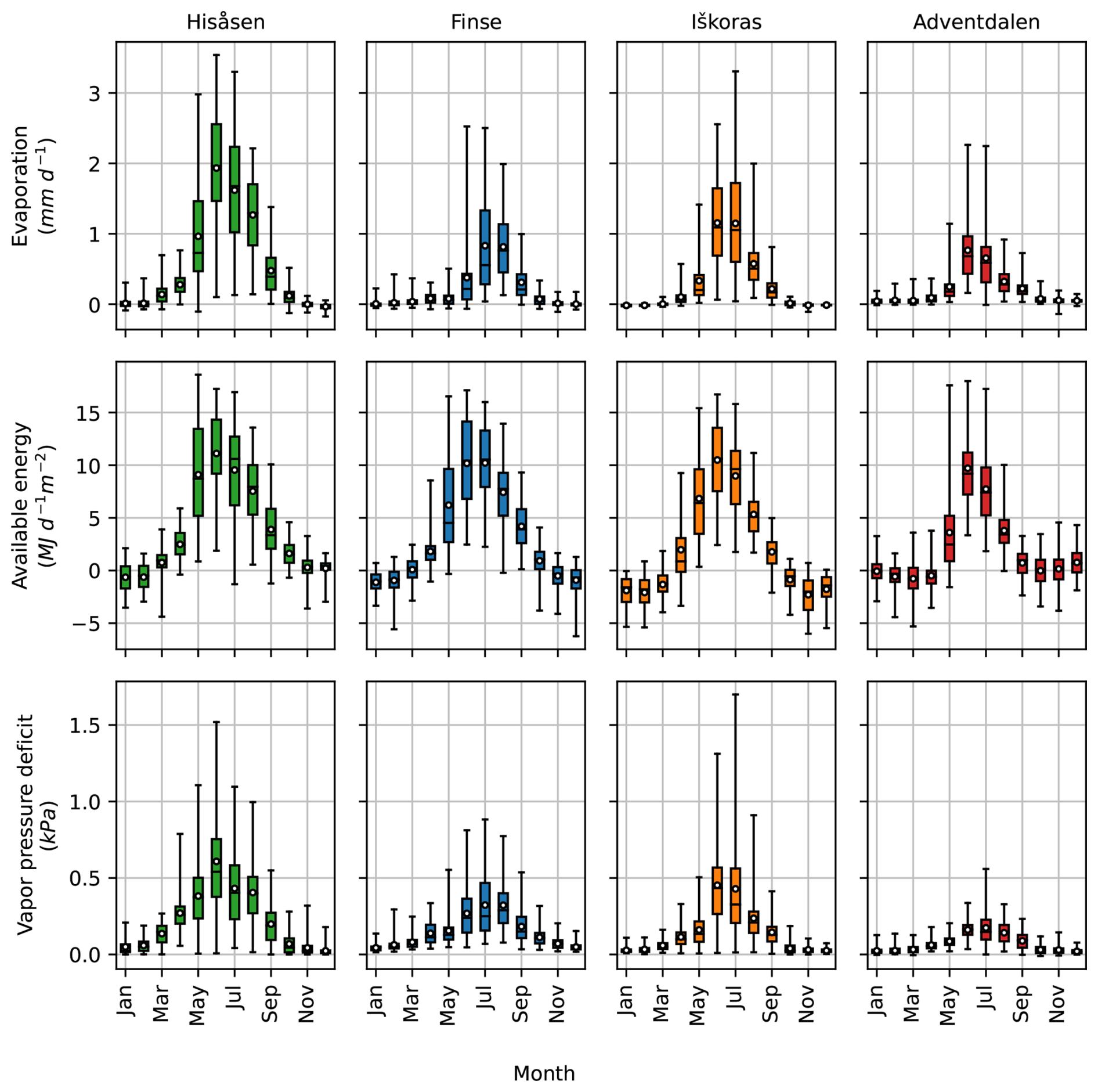
Figure 5 Daily evaporation in mm d⁻¹ (upper row), available energy in $\mathrm{MJ}{\mathrm{m}}^{-\mathrm{2}}{\mathrm{d}}^{-\mathrm{1}}$ (middle row) and vapour pressure deficit in kPa (lower row) for each month at the four sites. For each month, the box plot represents median, 25- and 75 quantiles, and whiskers represent minimum and maximum values. The mean is represented by a white dot. Daily values are cumulative values of half-hourly values for evaporation and available energy, and daily mean for vapour pressure deficit.

3.2 Magnitudes of evaporation

Daily evaporation rates showed a clear seasonal pattern, with lower values in the snow-covered season and higher values in the snow-free season. Across the sites, mean daily evaporation (averaged over season) ranged from 0.0 to 0.1 mm d⁻¹ in the snow-covered season, from 0.2 to 0.4 mm d⁻¹ in the shoulder season and from 0.5 to 1.0 mm d⁻¹ in the snow-free season. In the shoulder and snow-free season, the magnitudes of mean daily evaporation followed the gradient in mean annual temperature, with the highest evaporation at Hisåsen and lowest at Adventdalen, while in the snow-covered season there were only minor differences between the sites. Looking at the distribution of daily evaporation per month of the year (Fig. 5, upper row), we found that the mean daily evaporation was highest in the summer months, June–August, at all sites. However, the month of the highest mean daily rates were slightly different between the sites. The mean daily evaporation peaked in June at Hisåsen and Adventdalen, June/July at Iškoras and July/August at Finse. Comparing across sites, evaporation was highest at Hisåsen, with mean daily evaporation of 1.9 mm d⁻¹ (June), compared to 0.8 mm d⁻¹ at Finse (July/August), 1.2 mm d⁻¹ at Iškoras (June/July), and 0.8 mm d⁻¹ at Adventdalen (June).

The seasonal pattern of available energy and vapour pressure deficit followed a similar seasonal pattern, with lower values in winter and higher during summer (Fig. 5, middle and lower row). Mean daily available energy ranged from −1.6 to 0.6 MJ d⁻¹ in the snow-covered season, from 1.2 to 5.0 MJ d⁻¹ in the shoulder season, and from 6.1 to 7.0 MJ d⁻¹ in the snow-free season. Mean daily vapour pressure deficit ranged from 0.04 to 0.12 kPa in the snow-covered season, from 0.03 to 0.15 kPa in the shoulder season, and from 0.14 to 0.35 kPa in the snow-free season. Available energy peaked in June for all sites, while vapour pressure deficit peaked in either June, July, or August depending on site.

Across the sites, we found a large variation in the role of evaporation in the vertical water balance, due to a higher variation in precipitation (Table 1) than in evaporation. The evaporation ratio, i.e. the ratio of evaporation to precipitation, was highest at Adventdalen, the site with the lowest precipitation, and lowest at Finse, the site with the highest precipitation. For individual months, the evaporation ratio was occasionally over 100 % at all sites, and up to 400 % at Adventdalen (Fig. 6). At Finse, the monthly evaporation ratio was generally below 40 %, except in August 2021 when evaporation was 124 % of the precipitation. At Adventdalen, the monthly evaporation ratio was typically higher than 100 % in May, June, and July. Considering the warm season (May–September), the total evaporation was up to 72 % of the precipitation in the same months (at Adventdalen in 2015). The mean warm season evaporation ratio was lowest at Finse (20 %), intermediate at Hisåsen (48 %) and Iškoras (47 %) and highest at Adventdalen (58 %). The mean annual evaporation ratio ranged from 9 % to 30 % of MAP (Fig. 6), and the evaporation ratio increased with decreasing MAP across sites.

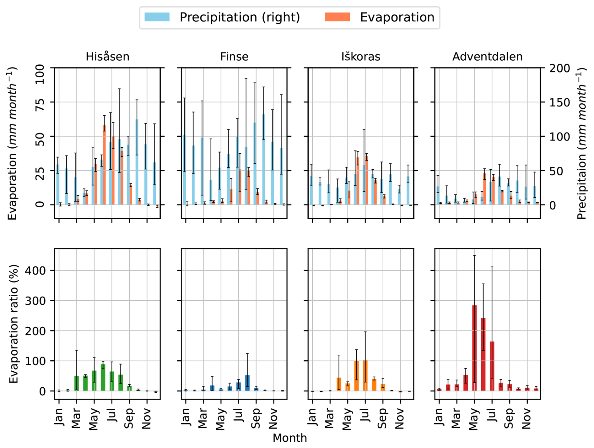
Figure 6 Mean monthly evaporation and precipitation in mm (upper row), with error bars representing minimum and maximum values, and mean monthly evaporation ratio in % (lower row), with error bars representing minimum and maximum values.

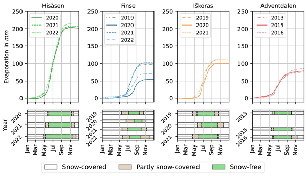
Overall, annual evaporation followed the gradient in mean annual temperature, with evaporation increasing with increasing temperature (Fig. 7). The highest annual evaporation was found at the Hisåsen site, with mean annual evaporation amounting to 208 mm, followed by 107 mm at Iškoras, 81 mm at Finse and 80 mm at Adventdalen. Interannual variability in evaporation was generally low. At Hisåsen, Iškoras and Adventdalen, annual evaporation deviated less than 10 % from the mean. However, at Finse, the interannual variability was larger, with evaporation in 2020 being 34 % lower and in 2021 27 % higher than the mean of all four years.

We found that some site-specific interannual variability in evaporation corresponded with the interannual variability of the end of the snow-covered season. At Hisåsen, Finse and Iškoras the year with the lowest annual evaporation corresponded to the year with the longest lasting snow cover in spring (Fig. 7). Accordingly, at Hisåsen and Finse, the year with the highest annual evaporation corresponded to the year with the earliest snow cover melt-out. To assess whether the lower annual evaporation in years with a long-lasting snow-cover was mainly caused by a shorter evaporative season or if years with a longer lasting snow-cover had lower evaporative demand in the snow-free season, we compared weekly values of evaporation, incoming solar radiation and vapour pressure deficit for overlapping weeks in the snow-free season of each year. The comparison was set up as an ANOVA-analysis for each variable, using a significance level of p=0.05. We found that weekly evaporation rates did not differ significantly between years, nor were there significant differences in incoming solar radiation or vapour pressure deficit. Comparing across sites, a larger interannual variability in snow-cover duration in spring corresponded with a larger interannual variability in evaporation, with Finse showing the highest interannual variation.

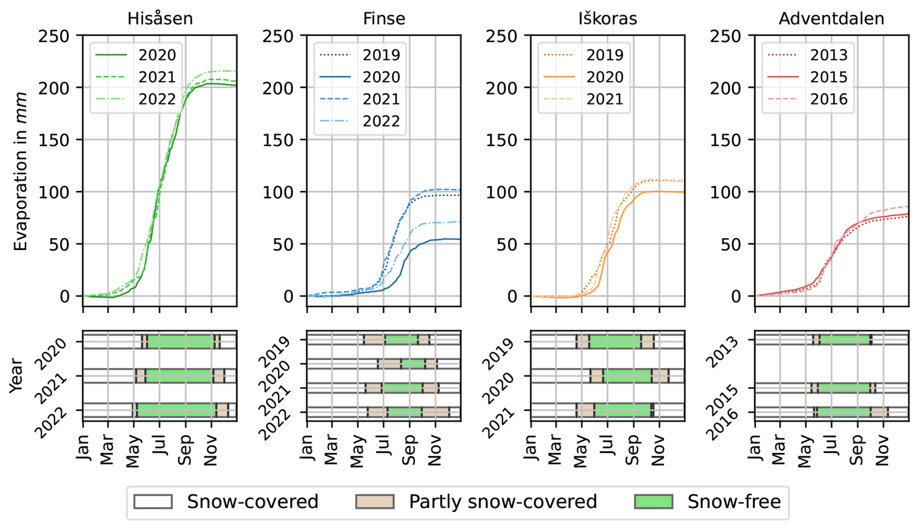
Figure 7 The upper row shows cumulative evaporation in mm (upper row) for the years 2019 (dotted lines), 2020 (dashed lines) and 2021 (solid lines) for sites Hisåsen (green), Finse (blue) and Iškoras (orange), and the years 2013 (dotted lines), 2015 (solid lines) and 2016 (dashed lines) for Adventdalen (red). The bars in the lower row represents the time of the year when the ground is either snow-covered (white bar) partly snow-covered (beige bar) or snow-free (green bar).

The mean annual evaporation at our sites (80–208 mm), was in the lower range of the mean annual evaporation at the selected FLUXNET2015 sites (45–385 mm), despite being in the mid-range of mean annual temperature. Furthermore, we found no significant linear relationship between annual evaporation with mean annual temperature when including the 14 FLUXNET2015 sites (Fig. F15). However, we found a significant increase in annual evaporation with mean temperature in the warm season (Fig. 8), with a slope of 16.4 mm °C⁻¹ (p<0.05). Still, all our four sites were below the trendline. We were unable to detect any pattern in the deviation from the regression line based on ecosystem type, however, the ecosystem types were not evenly distributed over the temperature range. For example, all forest sites were in the upper end of the temperature range.

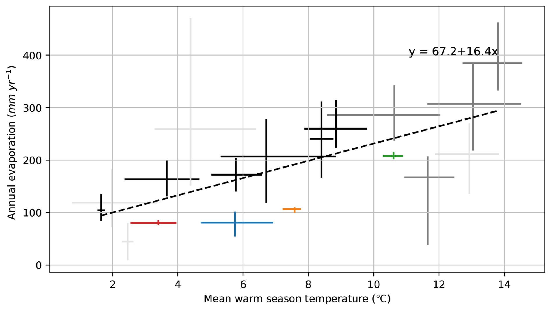
Figure 8 Annual evaporation of selected FLUXNET2015 sites above 60° N latitude (evergreen needle-leaf forest in dark grey, wetlands in black and other ecosystem types in light grey) compared to the study sites Hisåsen (green), Finse (blue), Iškoras (orange) and Adventdalen (red). The annual evaporation (in mm) on the y axis is plotted against mean May–September temperature (in °C), averaged over measured years, on the x axis. The bars represent minimum and maximum values of years in measurement periods, while the intersect represent the mean. The dashed line shows the linear regression line of mean warm season (May–September) temperature and annual evaporation (including both our four study sites and the fourteen FLUXNET sites).

4 Discussion

4.1 Controls on evaporation

Our results show that evaporation from northern latitude wetlands is mainly controlled by atmospheric evaporative demand, and furthermore, that the evaporative demand depends mainly on incoming solar radiation and vapour pressure deficit. On the sub-daily (hourly) timescale, vapour pressure deficit and incoming solar radiation had a strong correlation with evaporation, loaded high in the factor analysis on the same factors as evaporation, and had a high relative importance in the random forest model. Though vapour pressure deficit and incoming solar radiation had a high degree of shared variance, we found that evaporation was occasionally limited by low vapour pressure deficit despite available energy being high (Fig. 4). Especially at Finse and Adventdalen, where the climatic setting and oceanic influence lead to lower warm season temperatures and higher air humidity, the vapour pressure deficit was typically low, leading to constrained evaporation. At low vapour pressure deficit, more of the available energy was partitioned into sensible heat flux, as shown by the higher Bowen ratio for low vapour pressure deficit (Fig. F8). Additionally, we found that evaporation at Adventdalen in the snow-covered season was mainly controlled by vapour pressure deficit. The correlation to other controls was weak. This is likely due to the long polar night at Adventdalen with low variation in solar energy.

Other studies such as Liljedahl et al. (2011) and Helbig et al. (2020) have discussed the role of vapour pressure deficit in controlling northern latitude evaporation. Liljedahl et al. (2011) found latent heat flux to persistently exceed sensible heat flux when vapour pressure deficit was above 0.3 kPa for wet soils, and above 1.2 kPa for dry soils. We found a similar threshold at around 0.8–1.0 kPa (Fig. F8) with no clear effect of soil moisture content (Fig. F9). Additionally, we found that the Bowen ratio continued to decrease with vapour pressure deficit at Iškoras and Finse while the midday mean Bowen ratio at Hisåsen levelled off at values just below 1 at high vapour pressure deficits. The higher Bowen ratio at Hisåsen during high vapour pressure deficit might be caused by a higher cover of vascular plants. Vascular plants close their stomata during periods of high vapour pressure deficit to prevent excessive water loss (Novick et al., 2016), resulting in reduced transpiration rates. At Finse, Iškoras, the footprints of the eddy covariance measurements have a higher percentage than Hisåsen of open water surfaces and non-vascular vegetation where the soil remains saturated most of the year (Fig. 2), and evaporation may continue to increase in response to the increased atmospheric evaporative demand as vapour pressure deficit increases. Helbig et al. (2020) found a varying response to increasing evaporative demand based on vegetation type, and showed that evaporation from boreal peatlands increased more than evaporation from boreal forests with increasing vapour pressure deficit. At Hisåsen, a few trees are present in the footprint, however it is unclear how they contribute to the total evaporation measured. Warren et al. (2018) found that overstory transpiration contributed less than 1 % to total evaporation of a boreal bog with sparse tree density in north-western Canada.

Our results indicate that evaporation during the snow-free season has a low sensitivity to surface conditions, apart from the effect of the surface on available energy. Overall, the evaporation dynamic in the snow-free season was well represented by the Penman-Monteith equation with a fixed site-specific surface conductance. We found no tendency for the relative error of the Penman-Monteith estimates or Bowen ratio to change with decreasing soil moisture content or time since rain (Figs. F5, F6 and F9), indicating that evaporation was not constrained by low soil moisture content at our sites. The tendency of larger relative error (model overestimation) at high soil water content at Finse was likely because the highest levels of soil moisture were only reached during or shortly after rain events, when vapour pressure deficit was very low. The Penman-Monteith model tended to overestimate evaporation during periods of low vapour pressure deficit (Fig. 4). Furthermore, we found no change in relative error with growing degree day (Fig. F7), indicating that the seasonal vegetation development has limited influence on the total evaporation. However, the transpiration response to leaf phenology and soil moisture may be hard to detect due to a larger soil and free water evaporation in the total evaporation measured. Other studies have found that vegetation type is an important predictor of high-latitude evaporation (Oehri et al., 2022). The low sensitivity to soil moisture and phenology at our sites agrees with the results of Kasurinen et al. (2014), who studied evaporation in 65 boreal and arctic eddy covariance sites and found that surface conditions exert strong control on the latent heat flux in mature forest, but has less influence in ecosystems with shorter vegetation such as grassland, wetlands, and tundra.

The four sites in this study can all be described as having well-watered soils throughout the year, and the measurement periods did not include substantial dry periods. Therefore, it is likely that the soil moisture content did not decrease to a level where it would restrict evaporation. However, as the surfaces at the sites included are heterogenous, evaporation may have been restricted by lower soil moisture in the drier parts of the footprint although not detectable in the observations due to averaging out by higher evaporation from wetter parts. Spence and Rouse (2002) found low Bowen ratios in wet years after large snowmelts in the Canadian shield subarctic terrain and increased over the growing season. Although this study did not specifically examine how the Bowen ratio changed with time since snowmelt, point measurements of soil water content (available at Hisåsen, Finse and Iškoras) indicated that soil moisture during the snow-free season was influenced more by individual rainfall events than by the time elapsed since snowmelt (Fig. F10). At Finse and Iškoras, the highest levels of soil moisture were found during and right after rain events, while at Hisåsen the relation of soil moisture and time since rain was unclear. We also found no clear relationship between years with greater snow accumulation (Fig. F16) and level of soil moisture at the start of the snow-free season. Other studies have found contrasting results regarding the sensitivity of evaporation to soil moisture content in northern latitude ecosystems. Westermann et al. (2009) and Liljedahl et al. (2011) found that the Bowen ratio in a high-arctic tundra site and at an Arctic coastal wetland, respectively, decreased with higher soil water content, i.e., latent heat flux was favoured over sensible heat flux when soil water content was high. Ohta et al. (2008) found soil moisture to be a strong control on interannual variation in evaporation from a deciduous needle leaf forest in eastern Siberia, while Sabater et al. (2020) found that temporal changes in soil moisture did not affect evaporative fluxes in subarctic deciduous woodland. Transpiration and soil evaporation typically decrease with soil moisture content below a certain threshold (Shutov et al., 2006).

We found that the presence or absence of snow on the surface had a large effect on evaporation rates, especially during spring, when the atmospheric evaporative demand was high. The amount of accumulated snow during the winter can affect the warm season flux budget. Pirk et al. (2023) investigated the effect of snow cover duration on annual evaporation, in a study of water and carbon fluxes at Finse. In 2020, a year with one month delay in snow cover melt-out, the annual evaporation was reduced by 50 % compared to 2021 – a year with normal snow cover duration. Stiegler et al. (2016) found that, in a year with above average snow accumulation, accumulated growing season latent heat flux was reduced by 33 % in a high arctic wet fen in Zackenberg, Northeast Greenland, while it increased by 24 % in a nearby dry heath at the expense of sensible heat. We found that that sites with lower interannual variation in snow-cover duration have lower interannual variation in evaporation, and that a longer lasting snow-cover is typically associated with lower annual evaporation.

The dynamics of evaporation in the snow-free season was well represented by the Penman-Monteith equation, despite using a fixed surface conductance parameter. Predicting the magnitude, however, depends on finding a suitable value for surface conductance. The Penman-Monteith equation assumes surface energy balance, i.e. available energy is partitioned into either sensible or latent heat flux, whereas the measured fluxes do not amount to the measured available energy at the sites. Accordingly, the surface conductance parameter acts to compensate for the lack of for energy balance closure. By optimizing the surface conductance parameter using the sum of observed sensible and latent heat as available energy (i.e. forcing energy balance closure), we found higher values of surface conductance, with less variation between sites (0.0028–0.0044 m s⁻¹ compared to 0.000–0.0028 m s⁻¹ when the difference between net radiation and soil heat flux was used as available energy). Lack of energy balance closure is not uncommon for eddy covariance sites, and can be caused by e.g. unmeasured storage terms, large scale exchange processes, and landscape heterogeneity (Foken, 2008; Stoy et al., 2013). In the snow-free season, energy balance closure varied from 0.7 at Hisåsen to around 0.5 at Finse, Iškoras and Adventdalen (Tables 3 and F1). When including data for the whole year, the degree of energy balance closure was lower at Finse and Iškoras (Fig. F2). This might be partly due the energy used for snow melt, which is not accounted for in the energy balance calculation. As Finse on average accumulated more than the double amount of snow (in mm water equivalent) as the other sites (Fig. F16), energy spent on snow melt will have a lower effect on the full year energy balance of the other sites. Additionally, weather conditions associated with low energy balance closure may be more common in winter.

4.2 Magnitudes of evaporation

At the four Norwegian eddy covariance sites studied, we found that the mean annual evaporation ranged between 80–208 mm. This is at the lower end and below the range of pan evaporation rates measured at 42 sites in Norway between 1967 and 1972 (Hetager and Lystad, 1974). The pan evaporation sites were mostly located at lower altitudes with higher temperatures. For the five pan sites with a mean annual temperature in the reference period 1961–1990 below 3 °C (data from MET Norway), annual pan evaporation ranged from 250–315 mm (mean annual temperature was 1.0–2.4 °C).

The magnitudes of annual evaporation at our four eddy covariance sites were within the range found at northern latitude eddy covariance sites in FLUXNET2015 (45–385 mm). Including the FLUXNET2015 sites in the data sample, annual evaporation showed a strong relation to mean temperature in the warm season (May–September). However, all four Norwegian sites ended up below the regression line. Grouping the site ecosystem types into wetland and forest sites did not reveal any pattern that could explain the deviation seen. However, the ecosystem types were not evenly distributed in the temperature range. Another possible explanation for the deviations is the degree of continentality, where sites in more oceanic climates are influenced by maritime moist air masses and have lower vapour pressure deficit for the same temperatures compared to sites in more continental climates.

We found a large variation in the role that the evaporation plays in the vertical water balance. At Finse, the annual evaporation was less than 13 % of the annual precipitation, while at Adventdalen evaporation amounted to more than 28 % of the precipitation. The large variation in the evaporation ratio (evaporation as a fraction of precipitation) was caused by a high variation in annual precipitation across sites with evaporation varying less. The wettest site, Finse, is also the site with the lowest evaporation. The evaporation ratio is thus mainly controlled by precipitation. As the precipitation data used in this study have not been corrected for potential under-catch, the precipitation might be underestimated, especially in the months when precipitation falls as snow. Thus, the estimated evaporation ratios might be overestimated, especially for months in the cold season as well as annual estimates. The evaporation ratio for the warm season is less affected by precipitation under-catch when precipitation falls as rain (Wolff et al., 2015).

4.3 Evaporation in a warmer climate

Our results suggest that evaporation from northern latitude wetlands will increase in a warmer climate with the expected reduction in snow-cover duration (Rizzi et al., 2017) and increased vapour pressure deficit (Douville et al., 2021). We found that site-level variation in annual evaporation was linked to spring snow-cover melt out timing, whereas we did not find any significant difference in the evaporative demand between years for overlapping periods (weeks) of the snow-free season. Although our dataset only included 3–4 years of data per site, it is reasonable to conclude that the snow-cover melt out date has a notable effect on annual evaporation. The mean snow melt-out dates across all sites varied from 23 May to 14 July, a period of the year when incoming solar radiation typically is high. An earlier snow cover melt out date implies more solar radiation will be absorbed by the surface (lower albedo as compared to a snow-covered surface), enhancing an early start of the growing season. The timing of the start of the snow covered season in autumn is less likely to affect the evaporation, as the evaporative demand is typically low this period of the year.

The study finds that low vapour pressure deficit is likely a constraining factor for evaporation at northern latitudes. Thus, it is likely that evaporation will increase with the expected increase in atmospheric demand through an increase in vapour pressure deficit in response to global warming.

The response of the ecosystem evaporation to increased evaporative demand will, however, depend on soil moisture availability (Novick et al., 2016). Though we did not observe any soil moisture constrains on evaporation, evaporation was regularly exceeding precipitation in May, June, and July at Adventdalen, which had the lowest precipitation, and was typically around 50 % of precipitation in the warm season. The soil moisture availability therefore depends on precipitation and/or melt water from preceding months. An earlier snow-cover melt-out and increased evaporation in spring, might lead to lowered soil moisture availability later in the season, potentially limiting evaporation in anomaly warm and dry years.

5 Conclusions

The study investigated controls and magnitudes of evaporation from four northern latitude wetlands in Norway. Our analysis show that the hourly evaporation in the snow-free season is mainly controlled by the atmospheric evaporative demand, which again is mainly controlled by incoming solar radiation and vapour pressure deficit. We found that the sensitivity of the Bowen ratio to vapour pressure deficit varied between sites. At the site with a higher cover of vascular plants, midday mean Bowen ratio levelled off at values just below 1 at vapour pressure deficits exceeding 1 kPa, while it continued to decrease with vapour pressure deficit at the sites with a larger cover of open water and non-vascular vegetation. The results indicate that the evaporation had a low sensitivity to phenology and observed changes in soil water content. We found that the mean daily evaporation was highest in June–August at all sites. However, the timing of the highest mean daily rates were slightly different between the sites. Mean annual evaporation ranged from 80 to 208 mm and increased with the spatial gradient in the warm season mean temperature. We found that sites with lower interannual variation in snow-cover duration have lower interannual variation in evaporation, and that a longer lasting snow-cover is typically associated with lower annual evaporation. The magnitudes of annual evaporation at our four Norwegian eddy covariance sites were within the range found at the northern latitude eddy covariance sites in FLUXNET2015, but in the lower range when considering the spatial gradient in the warm season mean temperature. The variability in ET found across our sites underpins the pressing need for additional in-situ measurements. These data-scarce regions are projected to experience strong climate warming, which can feed back to other components in the Earth system.

Appendix A: Climate reference data

Mean annual precipitation (MAP) and temperature (MAAT) listed in Table A1 are averages over the climate reference period 1991–2020 from the nearest MET Norway weather station. Data from the nearest weather station is used to estimate MAP and MAAT values for each site (Table 1) and to compare the monthly temperature and precipitation in the measurement periods to that of the climate reference period (Fig. 3). The nearest weather station to Hisåsen is “SN210 – Trysil Vegetasjon” (357 m a.s.l., precipitation and temperature). For Finse, the weather station is collocated with the eddy covariance station and climate reference data listed is from this station. For Iškoras, the nearest weather stations are “SN97251 Karasjok – Markannjarga” (131 m a.s.l., precipitation and temperature), and “SN97710 Iskoras” (131 m a.s.l., temperature only). An altitude-based weighted average between the two nearest weather stations is used to determine the mean annual and monthly values for Iškoras (380 m a.s.l.) in Fig. 1 and Table 1.

Table A1 Coordinates, altitude, mean annual precipitation (MAP) and temperature (MAAT) for weather stations used to describe the climatic context of the sites in this study. MAP and MAAT are averages over the climate reference period 1991–2020. Based on data from The Norwegian Meteorological Institute.

Appendix B: Classification of precipitation as snow, sleet or rain

To classify precipitation we applied a simple temperature-based climate indicator, as in Kuya et al. (2024), where precipitation is classified as snow (mean daily T≤−1 °C), sleet (−1 °C $>T<\mathrm{1}$ °C) or rain (T≥1 °C). Daily percentage in each category was then calculated as percentage of total daily precipitation. The monthly mean, for data in the respective measurement periods of the study sites , is summarized in Table B1. Daily precipitation and mean air temperature from the nearest MET Norway weather station (see Table A1) was used for the classification (SN180 for Hisåsen, SN25830 for Finse, SN97251 for Iškoras and SN99840). Similar values were found when using hourly data (not available at SN99840).

Table B1 Percentage of precipitation as snow, sleet of rain, average for each month in the respective measurement periods of the study sites (1 January 2020–31 December 2022 for Hisåsen, 1 January 2019–31 December 2022 for Finse, 1 January 2019–31 December 2021 for Iškoras and 1 January 2013–31 December 2013 and 1 January 2015–31 December 2016 for Adventdalen). The classification is based on daily precipitation and daily mean air temperature from the nearest MET Norway weather station.

Appendix C: Observed and gap-filled evaporation data

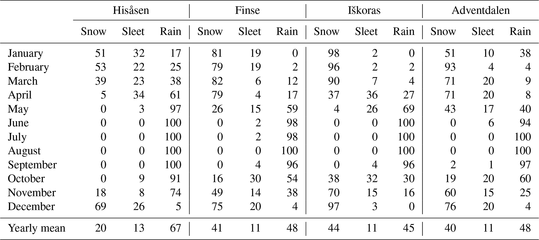
Table C1 Percentage of gap-filled and observed data for each site and each month. The values represent hours of gap-filled or observed data as percentage of total hours in each month.

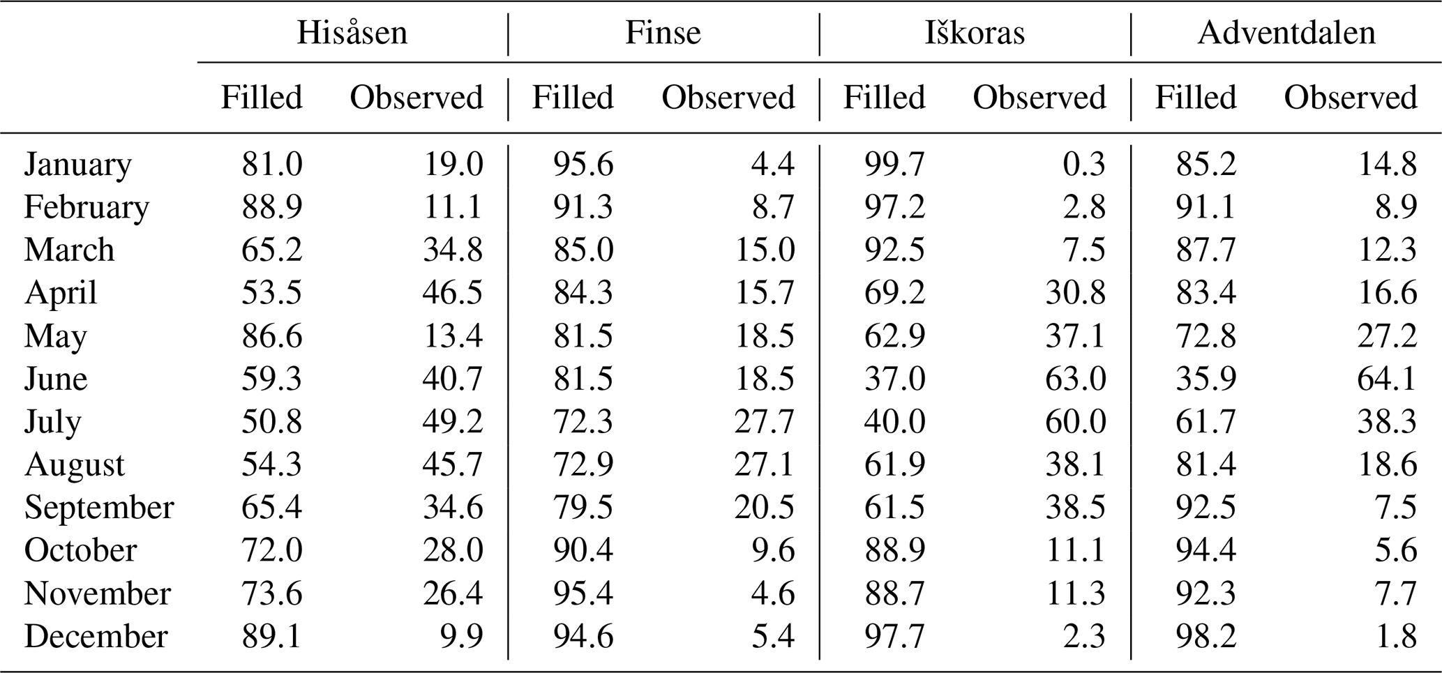
Figure C1 Time series of observed (coloured points) and gap-filled (grey points) evaporation in mm h⁻¹ for Hisåsen (green), Finse (blue), Iškoras (orange) and Adventdalen (red). Note that the axes, with time on the x axis and evaporation on the y axis, are not aligned between four study sites.

Appendix D: KMO-values in the factor analyses

Table D1 KMO-values in the factor analyses for each site, in the snow-free (top row) and snow-covered season (bottom row).

Appendix E: List of FLUXNET2015 sites used for comparison

Table E1 Sites in FLUXNET2015 selected for comparison. Selected sites are located at latitude above 60° N and have data licence CC-BY-4.0.

Appendix F: Supporting figures

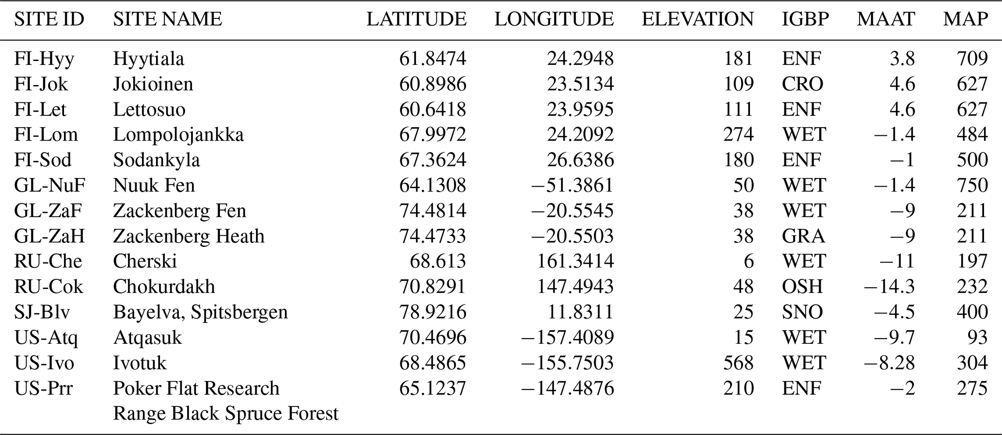
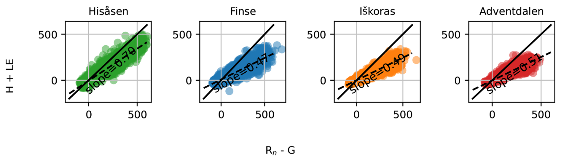
Figure F1 Energy balance closure in the snow-free season for Hisåsen (green), Finse (blue), Iškoras (orange) and Adventdalen (red). The energy balance is estimated from the slope of the linear regression of the sum of latent and sensible heat on the y axis against available energy (difference between net radiation and soil heat flux) on the x axis.

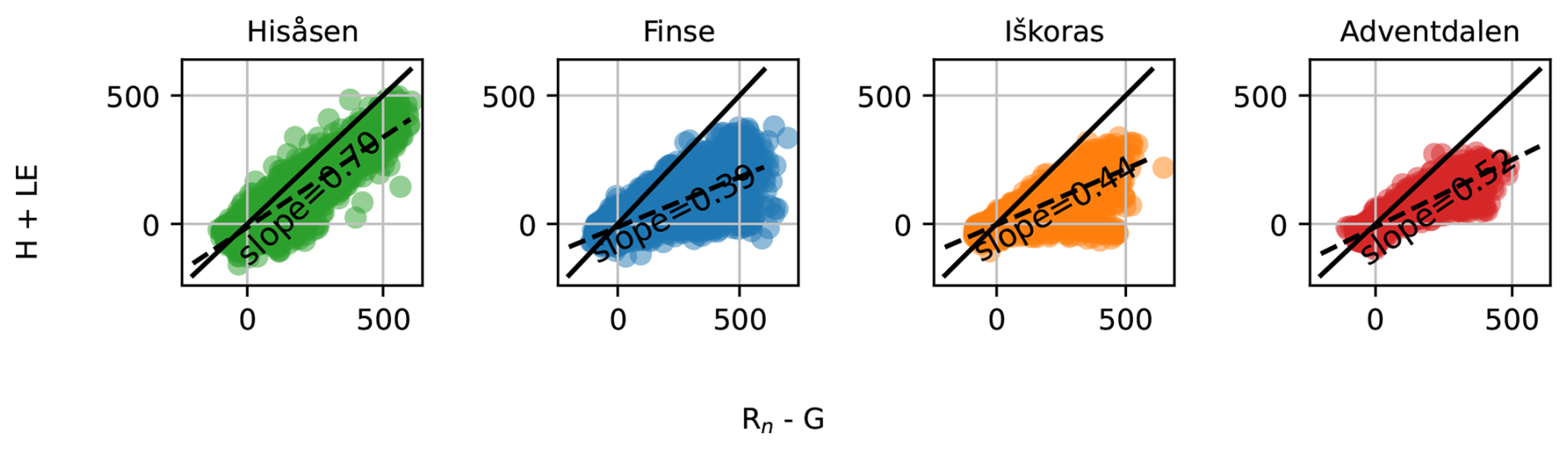
Figure F2 Energy balance closure (whole year) for Hisåsen (green), Finse (blue), Iškoras (orange) and Adventdalen (red). The energy balance is estimated from the slope of the linear regression of the sum of latent and sensible heat on the y axis against available energy (difference between net radiation and soil heat flux) on the x axis.

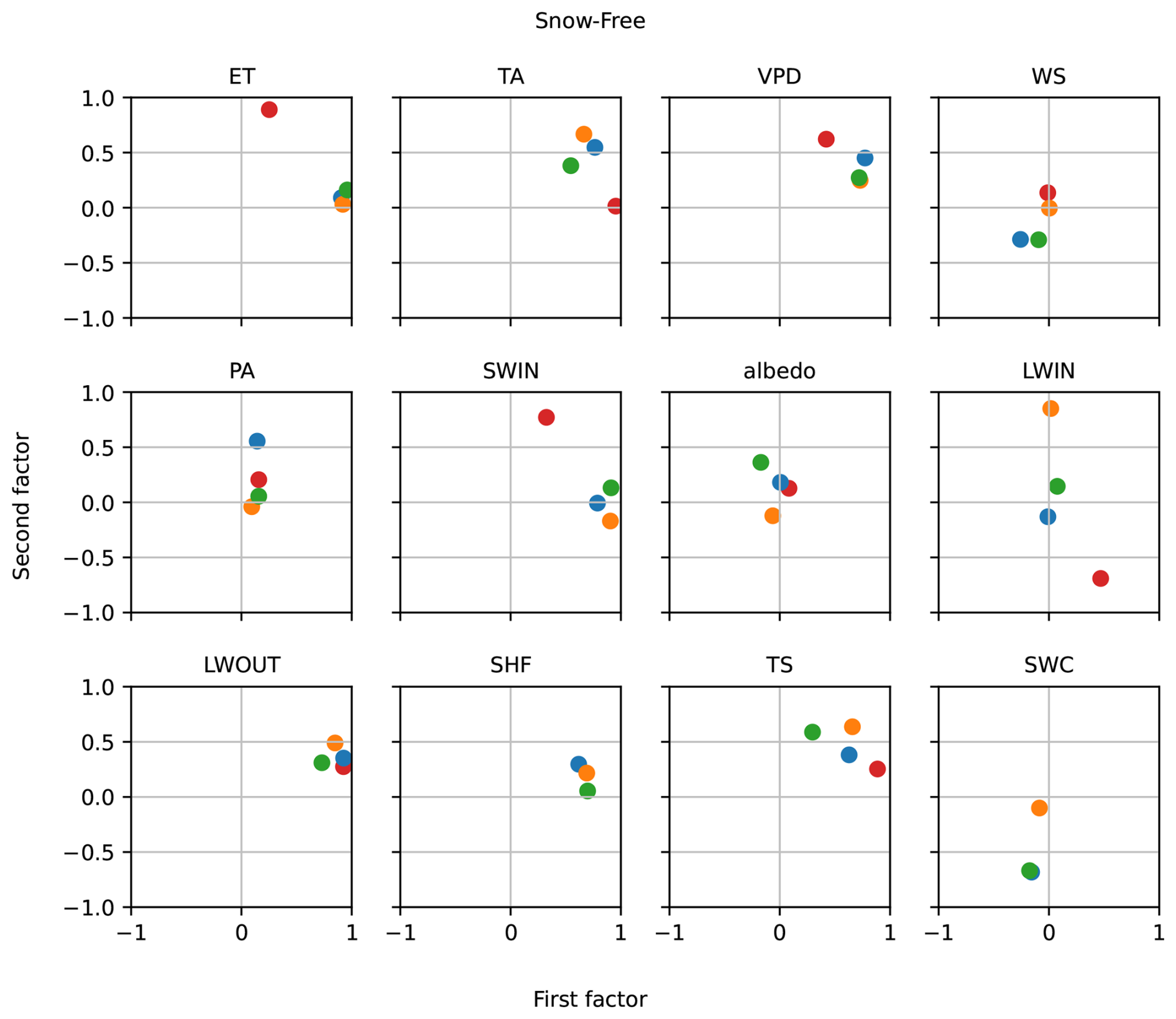
Figure F3 Factor loadings of first and second factor in the snow-free season, for each of the variables in the dataset. In each subplot the points represent results from Hisåsen (green), Finse (blue), Iškoras (orange) and Adventdalen (red).

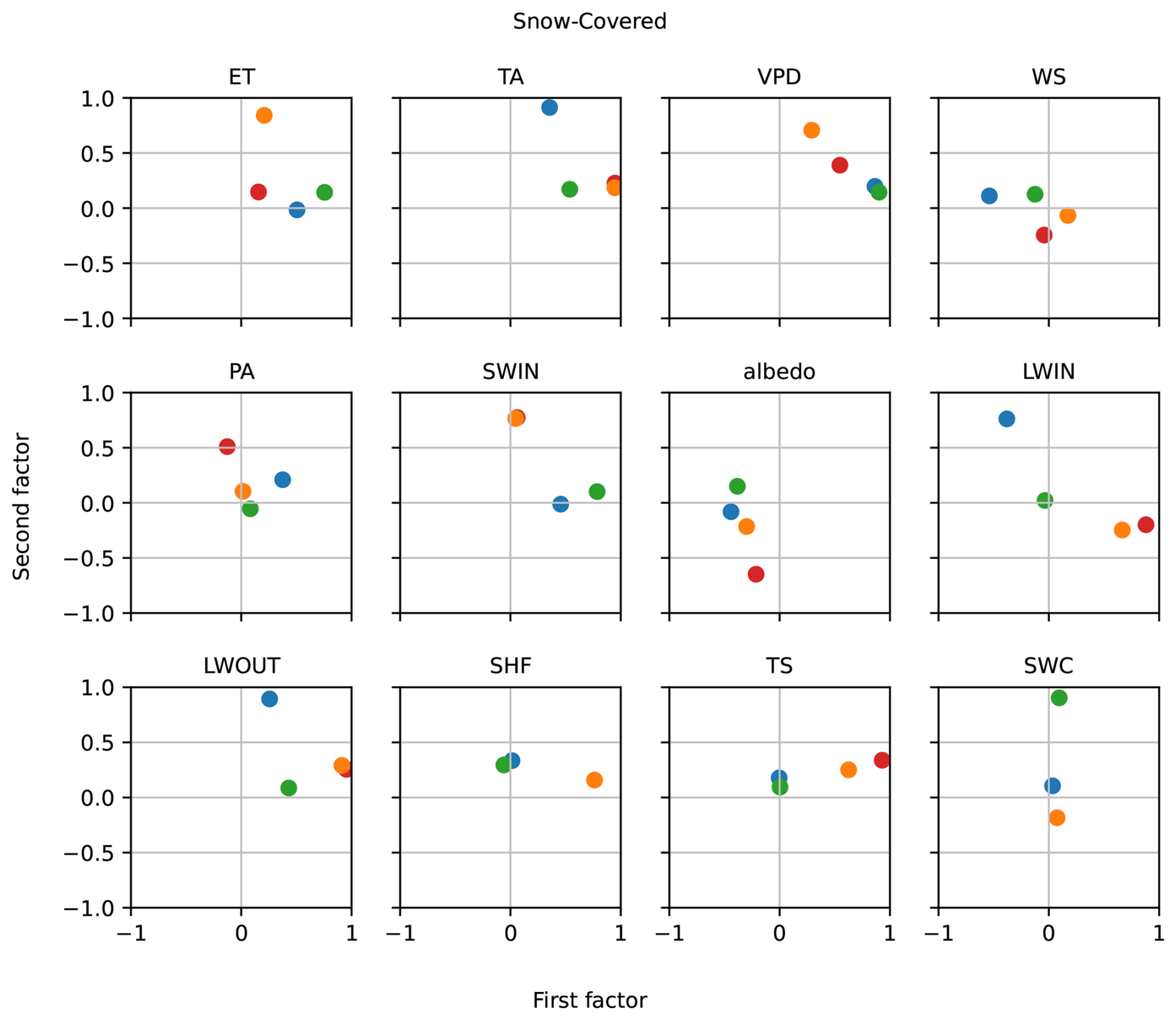
Figure F4 Factor loadings of first and second factor in the snow-covered season, for each of the variables in the dataset. In each subplot the points represent results from Hisåsen (green), Finse (blue), Iškoras (orange) and Adventdalen (red).

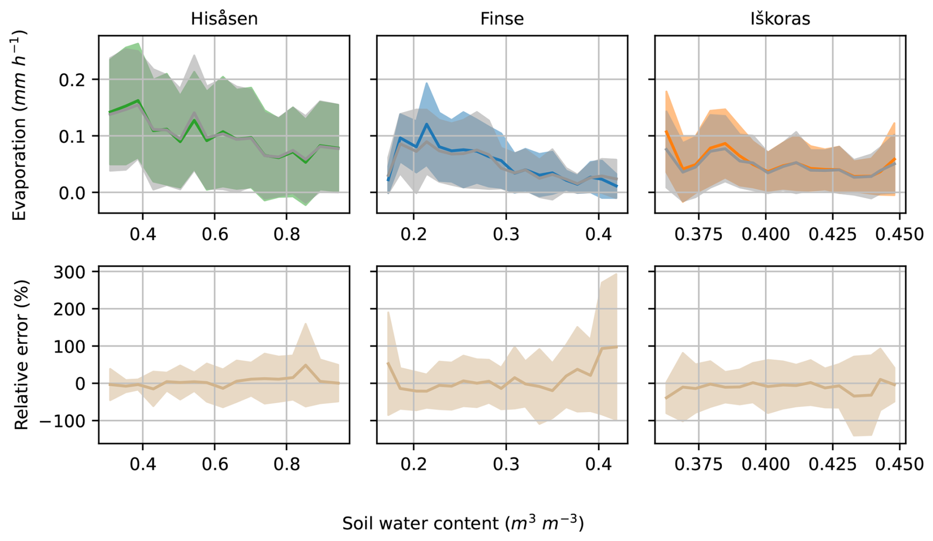
Figure F5 Sensitivity of observed (coloured) and modelled (grey) evaporation (upper row) and the relative error (lower row) to volumetric soil water content.

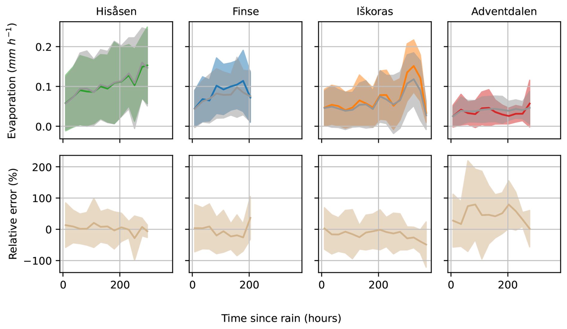
Figure F6 Sensitivity of observed (coloured) and modelled (grey) evaporation (upper row) and the relative error (lower row) to time since rain.

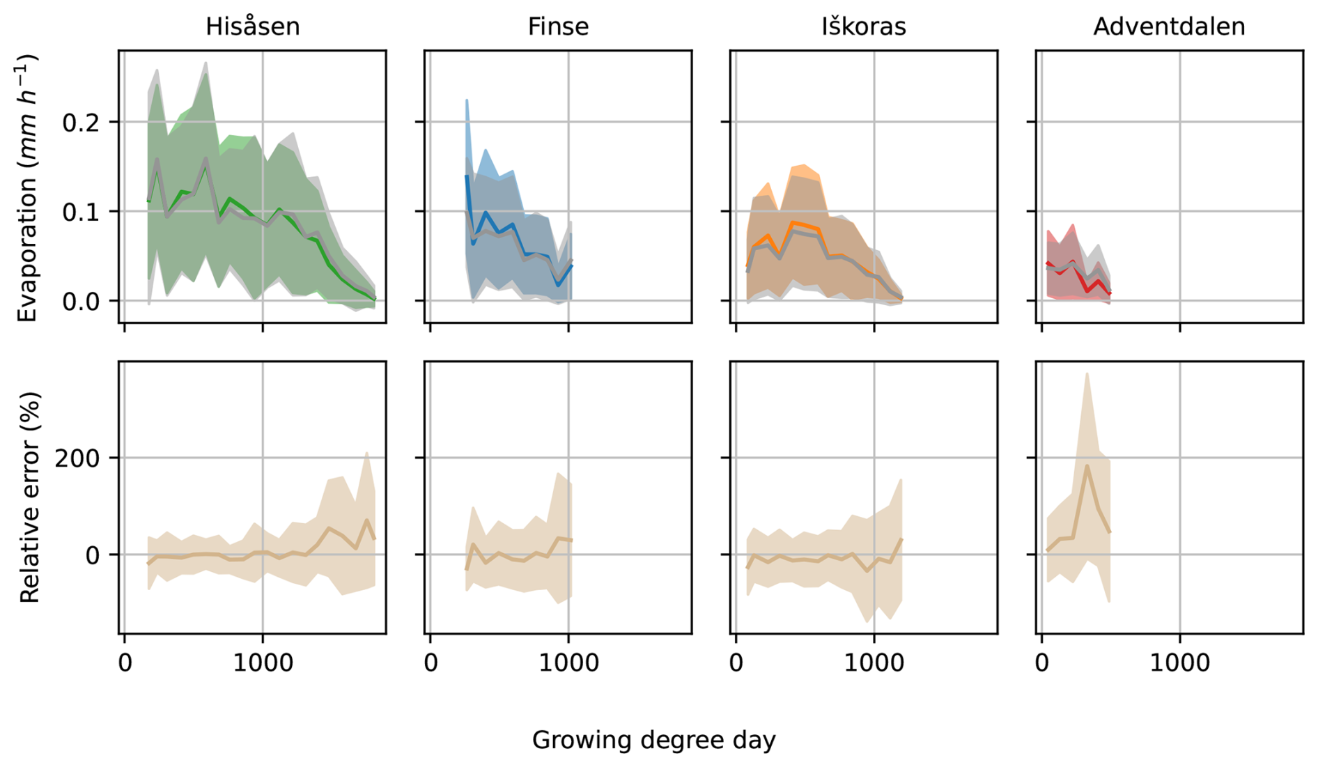
Figure F7 Sensitivity of observed (coloured) and modelled (grey) evaporation (upper row) and the relative error (lower row) to growing degree day.

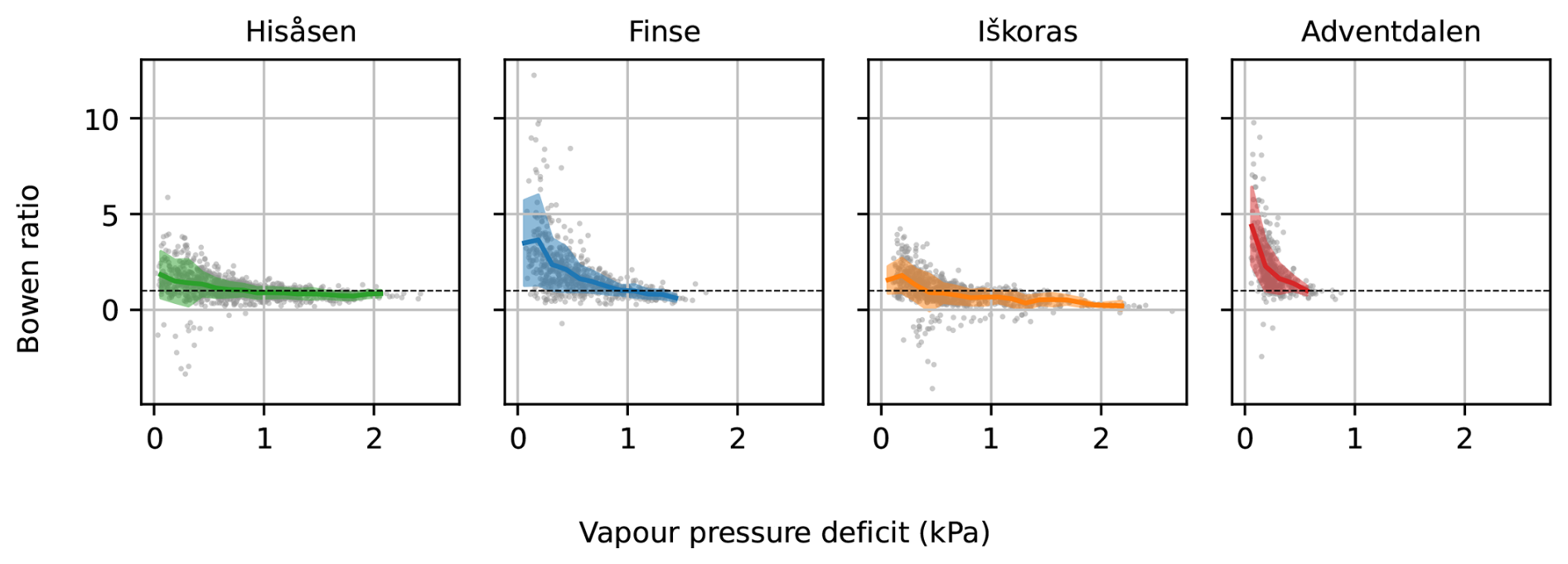
Figure F8 Sensitivity of Bowen ratio to vapour pressure deficit. The coloured areas show the mean (± standard deviation) midday Bowen ratio (grey dots) for 20 bins of vapour pressure deficit.

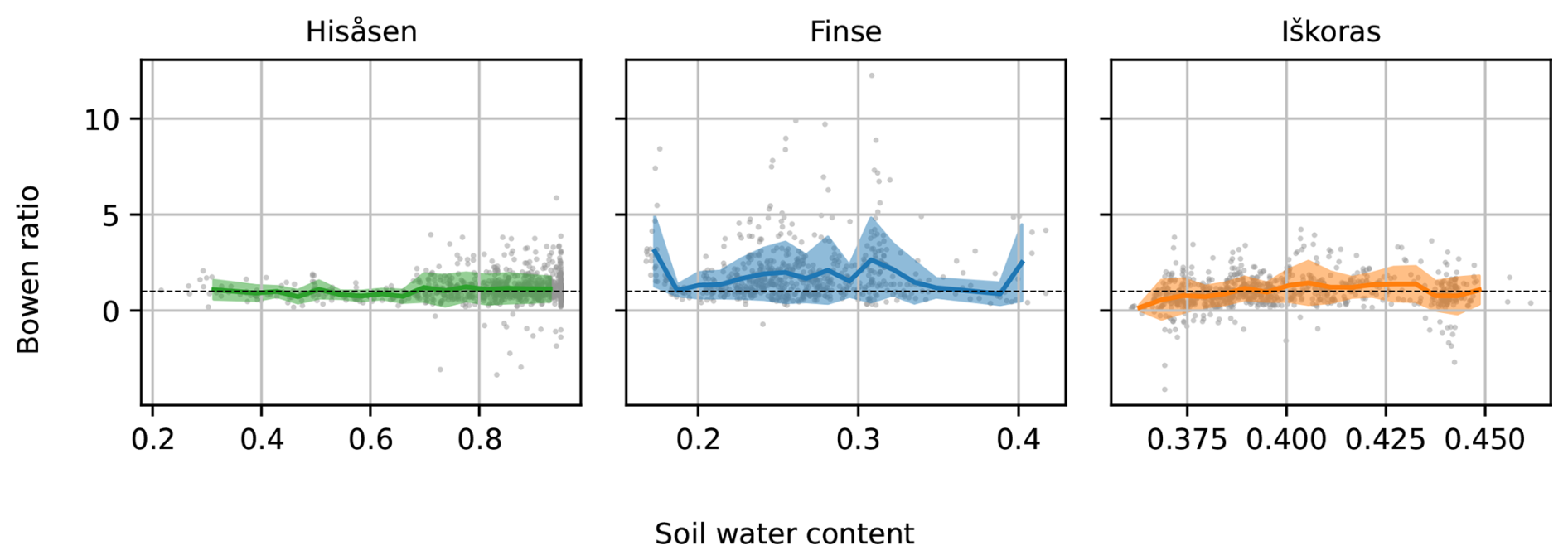
Figure F9 Sensitivity of Bowen ratio to volumetric soil moisture content. The coloured areas show the mean (± standard deviation) midday Bowen ratio (grey dots) for 20 bins of volumetric soil moisture content.

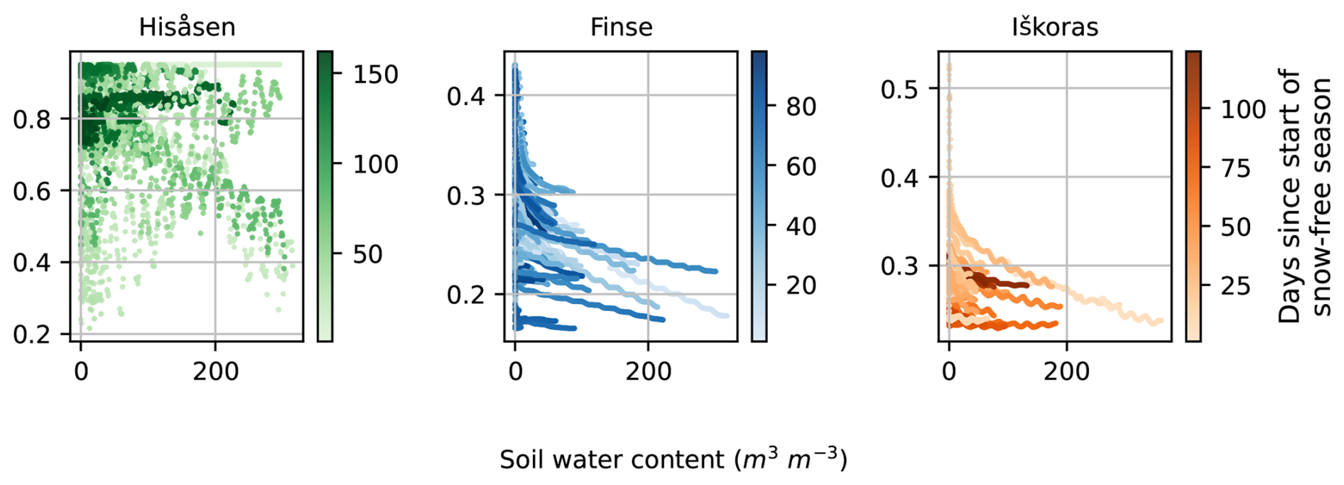
Figure F10 Scatter plot of time since rain (in hours) on x axis against soil water content in the snow-free season (in m³ m⁻³) on y axis, for Hisåsen in green, Finse in blue and Iskoras in orange. The shade of each colour (as represented by the colour bars) shows days since the start of the snow-free season, where lighter colours represent early snow-free season and darker colours represent late snow-free season.

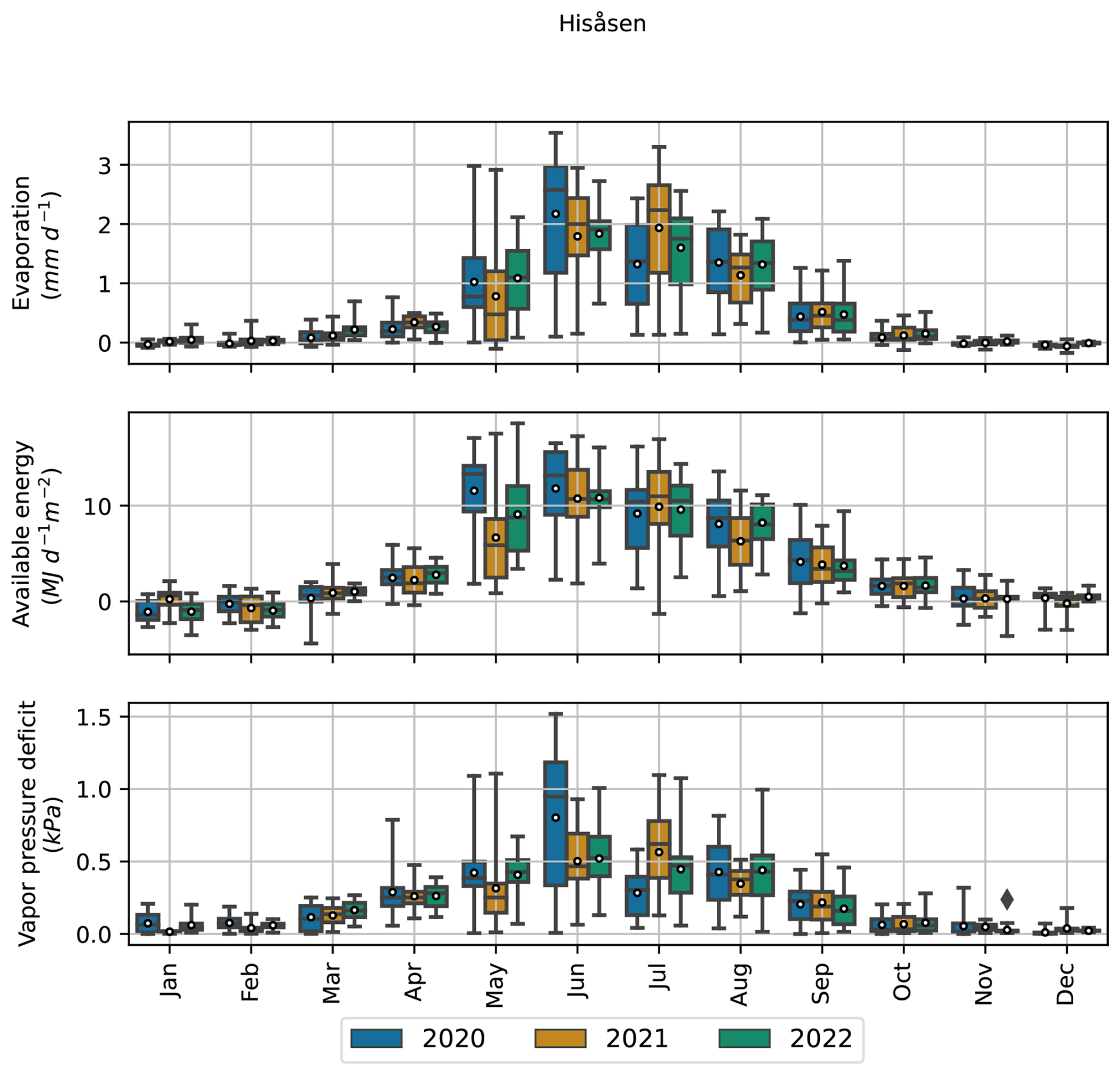
Figure F11 Distribution of daily evaporation (upper row, in mm d⁻¹), net radiation (middle row, in $\mathrm{MJ}{\mathrm{d}}^{-\mathrm{1}}{\mathrm{m}}^{-\mathrm{2}}$) and vapour pressure deficit (lower row, in kPa) at Hisåsen. For each month, the box plot represents median, 25- and 75 quantiles, and whiskers represent minimum and maximum values. The mean is represented by a white dot. Daily values are cumulations for evaporation and net radiation, and daily mean for vapour pressure deficit.

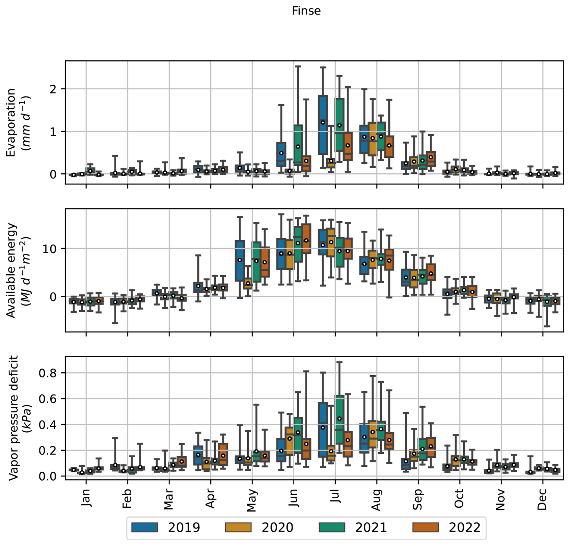
Figure F12 Distribution of daily evaporation (upper row, in mm d⁻¹), net radiation (middle row, in $\mathrm{MJ}{\mathrm{d}}^{-\mathrm{1}}{\mathrm{m}}^{-\mathrm{2}}$) and vapour pressure deficit (lower row, in kPa) at Finse. For each month, the box plot represents median, 25- and 75 quantiles, and whiskers represent minimum and maximum values. The mean is represented by a white dot. Daily values are cumulations for evaporation and net radiation, and daily mean for vapour pressure deficit.

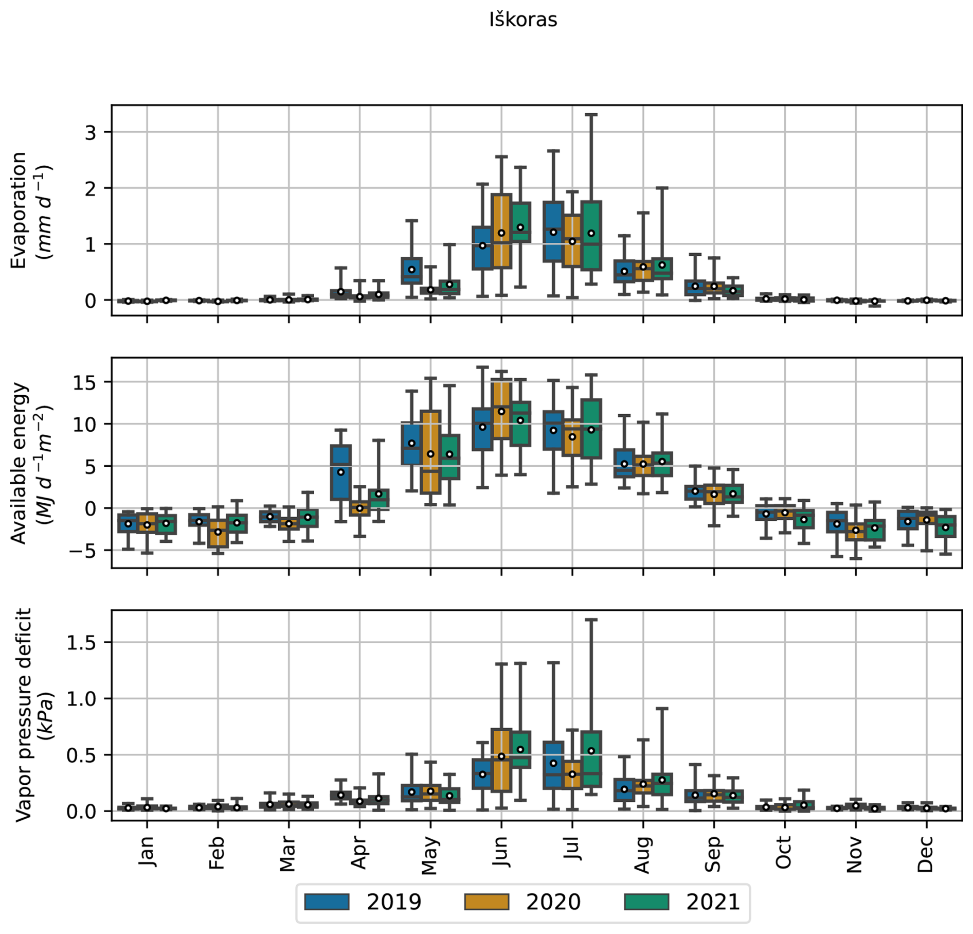
Figure F13 Distribution of daily evaporation (upper row, in mm d⁻¹), net radiation (middle row, in $\mathrm{MJ}{\mathrm{d}}^{-\mathrm{1}}{\mathrm{m}}^{-\mathrm{2}}$ and vapour pressure deficit (lower row, in kPa) at Iškoras. For each month, the box plot represents median, 25- and 75 quantiles, and whiskers represent minimum and maximum values. The mean is represented by a white dot. Daily values are cumulations for evaporation and net radiation, and daily mean for vapour pressure deficit.

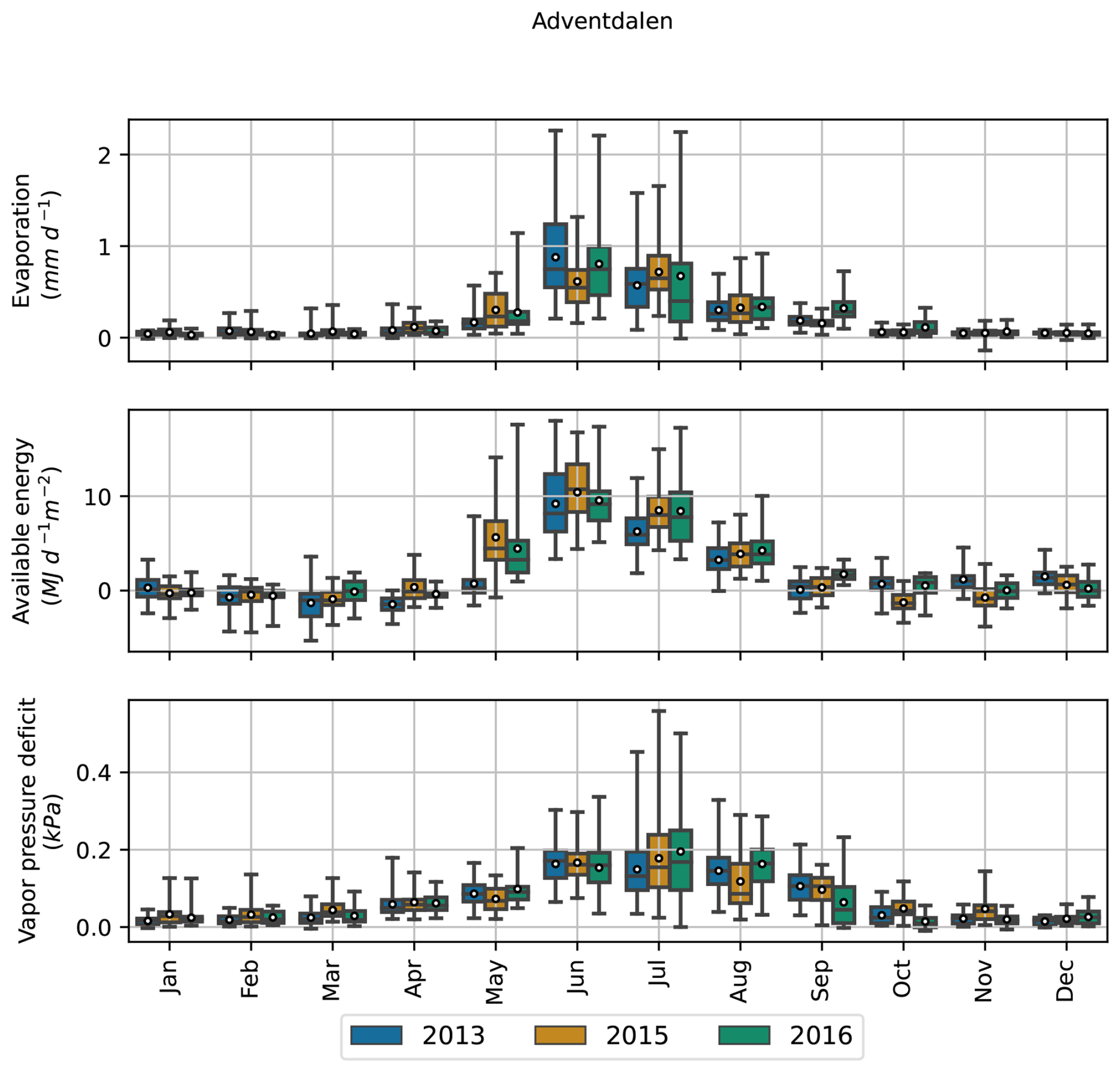
Figure F14 Distribution of daily evaporation (upper row, mm d⁻¹), net radiation (middle row, in $\mathrm{MJ}{\mathrm{d}}^{-\mathrm{1}}{\mathrm{m}}^{-\mathrm{2}}$) and vapour pressure deficit (lower row, in kPa) at Adventdalen. For each month, the box plot represents median, 25- and 75 quantiles, and whiskers represent minimum and maximum values. The mean is represented by a white dot. Daily values are cumulations for evaporation and net radiation, and daily mean for vapour pressure deficit.

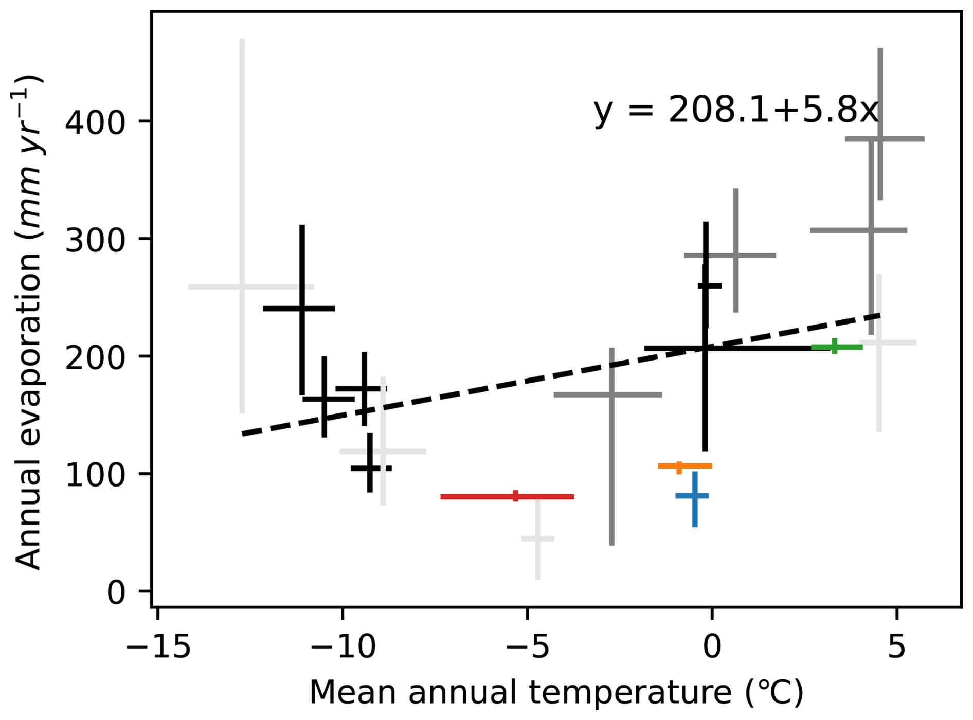
Figure F15 Annual evaporation of selected FLUXNET2015 sites above 60° N latitude (evergreen needle-leaf forest in dark grey, wetlands in black and other ecosystem types in light grey) compared to the study sites Hisåsen (green), Finse (blue), Iškoras (orange) and Adventdalen (red). The annual evaporation (in mm) on the y axis is plotted against annual mean temperature (in °C), averaged over measured years, on the x axis. The bars represent minimum and maximum values of years in measurement periods, while the intersect represent the mean. The dashed line shows the linear regression line of annual mean temperature and annual evaporation. The regression slope was not significant at p>0.05.

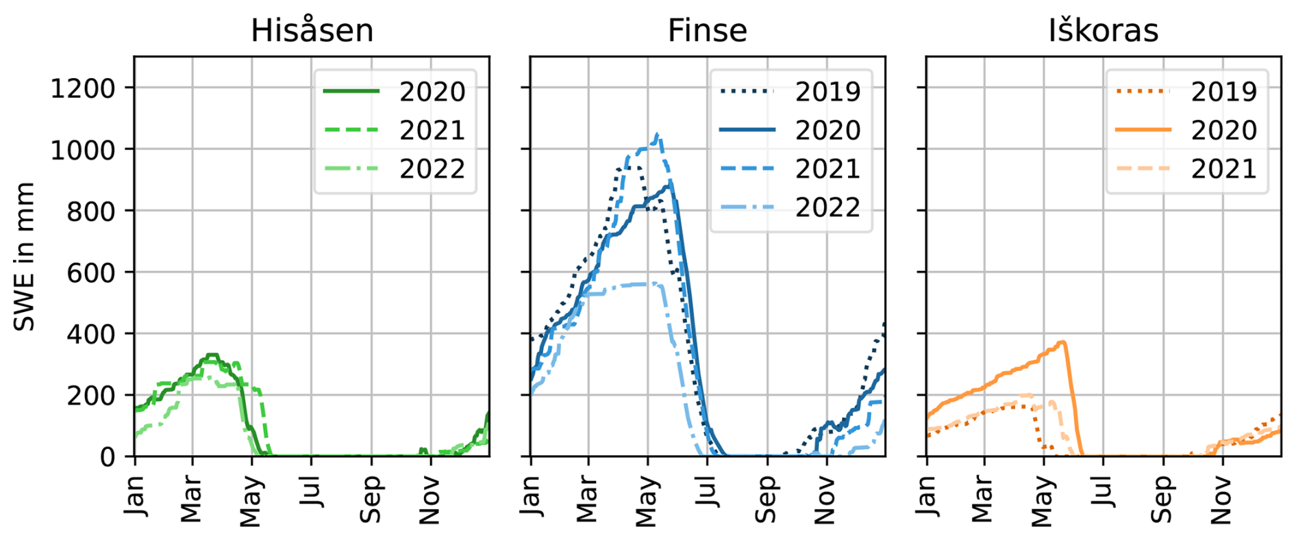
Figure F16 Model estimates of snow water equivalent (SWE), in mm, for each year of the respective measurement periods of Hisåsen in green, Finse in blue and Iškoras in orange. Model estimates for Adventdalen was not available. The data is downloaded from the seNorge website (http://www.senorge.no, last access: 26 January 2026), and is published under Norwegian Licence for Open Government Data (NLOD). Details on the SeNorge snow model can be found in Saloranta (2016).