Hydrologic model parameter estimation in snow-dominated headwater catchments using multiple observation datasets

Hydrologic models are often calibrated using streamflow alone, but increasing availability of in situ and satellite-based observations provide numerous opportunities to constrain model outputs and improve process representation. However, as new observation data emerges, it is often unclear whether calibration with additional data would inform or misinform streamflow prediction. Here, we carry out a multi-observational sensitivity and uncertainty analysis using the U.S. Geological Survey's National Hydrologic Model (NHM) in four headwater catchments in the Upper Colorado River Basin. We use seven different observational data products that pertain to discharge, snow water equivalent, snow-covered area, soil moisture, and evapotranspiration. Informative model parameters are identified using the Morris screening method across all data sets, followed by parameter estimation and streamflow performance assessment using a Latin Hypercube Sample Monte-Carlo filtering approach. Results show that an increased number of informative parameters are determined through the screening process with the use of observation data representing terms beyond streamflow, and that forcing corrections and rain-snow partitioning parameters are particularly impactful to the model fit to observations. Multi-objective Monte Carlo filtering reduces the number of behavioral parameter sets, and estimated parameter values can depend strongly on the observation data criteria. Evapotranspiration is informative for streamflow prediction across all catchments included in this study, but snow and soil moisture datasets are only informative in some. These results provide new insight into the variable value of alternative observation data for streamflow prediction and highlight challenges related to model/observation scale mismatches, compensating errors, and misinformative data.

1 Introduction

Improved scientific understanding of hydrologic processes, the growth of observational data, and advancements in computational power have led to the development of complex, spatially distributed hydrologic models (Beven, 1996; Gupta et al., 1998). These models help provide essential services to the public, such as water supply forecasting (Gorski et al., 2025), flood forecasting (Emerton et al., 2016; Hogue et al., 2000), drought monitoring (Hao et al., 2017; Pendergrass et al., 2020), and analysis of the impact of climate variability (Christensen et al., 2004). In the western United States, the Colorado River Basin is of particular interest because it provides an invaluable resource for 40 million inhabitants across several metropolitan and agricultural areas, and it is particularly vulnerable to climate variability and drought (Nash and Gleick, 1991; Wheeler et al., 2022). Mountainous headwater catchments provide up to 92 % of the total annual runoff for the entire Upper Colorado River Basin (UCRB) (Lukas and Payton, 2020); therefore, long term forecasting and climate related modeling in this domain is of particular interest to government agencies, water managers, and water rights holders. The value of hydrologic forecasts depends largely on how well the model performs with respect to observations; generally, model evaluation is carried out retrospectively to assess this. Long term discharge records (Q) are often the primary, if not only, observation against which hydrologic models are calibrated (Gupta et al., 1998; Mei et al., 2023). In recent decades, several different data products have emerged from satellite based or airborne missions, measuring or estimating variables such as soil moisture (SM), actual evapotranspiration (AET), snow-covered area (SCA), and snow water equivalent (SWE). These alternative observations have the potential to improve modeled streamflow performance when used to enhance model calibration; however, their inclusion has uncertain outcomes (Herrera et al., 2022).

Process based hydrologic models simulate several hydrologic processes and output time series of the state variables, which provides an avenue to compare with alternative observations. It has been widely reported that the use of gridded AET products improves streamflow performance when used in calibration (Dembélé et al., 2020; Huang et al., 2020; Liu et al., 2022; Livneh and Lettenmaier, 2012; Mei et al., 2023). Soil moisture (Mei et al., 2023; Oubeidillah et al., 2019) and terrestrial water storage (Hasan et al., 2025; Rakovec et al., 2016) have also been found to be informative. However, some studies have shown that in other cases, SM and AET can be misinformative or require bias correction depending on the product used (Kunnath-Poovakka et al., 2016; Széles et al., 2020). While in situ SWE observations have been shown to be informative for streamflow modeling in snow-dominated catchments (Livneh and Badger, 2020), there are several challenges associated with snowpack modeling, especially when semi-lumped model outputs are compared to point-scale measurements (Cho et al., 2022; Gelfan et al., 2004; Lundquist et al., 2013; Mazzotti et al., 2023). Remotely sensed SWE from the Airborne Snow Observatory (ASO) program has emerged within the last decade (Painter et al., 2016), with spatial patterning results that suggest in situ SWE observations are often not representative of the surrounding landscape (Herbert et al., 2024).

Multi-observational calibration studies have shown that streamflow prediction performance varies between datasets or combinations of multiple datasets (McCabe et al., 2005; Mei et al., 2023), and the results can depend on the catchment scale (Livneh and Lettenmaier, 2012). Uncertainties associated with calibration data can result in vastly different parameter estimates (Bárdossy and Singh, 2008), resulting in deleterious effects in flood hazard forecasting (Balbi and Lallemant, 2023), peak flow estimates (Bárdossy and Anwar, 2023), and climate change studies (Marshall et al., 2021). It has long been noted that observation quality is an important source of uncertainty in multi-objective calibration (Gupta et al., 1998). These challenges underscore the importance of developing multi-objective calibration, uncertainty quantification, and diagnostic procedures for models (Gupta et al., 2008).

Calibration and uncertainty analysis requires sampling parameters at a high density; however, this can become computationally expensive for models with many parameters and long run times (Razavi et al., 2021). Thus, a type of sensitivity analysis, parameter screening, often precedes further analysis to identify informative/highly sensitive parameters (Pianosi et al., 2016; Saltelli et al., 2019). Screening out non-informative parameters reduces the dimensions of the parameter space, which reduces sample sizes and computational demand. Keeping in mind the goal of calibration or uncertainty quantification, objective functions can be used in a sensitivity analysis, referred to as “identifiability analysis” when sensitivity is assessed relative to an objective function, following the terminology of Gupta and Razavi (2018). The value of alternative observations in an identifiability analysis context is relatively unexplored, and multi-objective methods are only briefly discussed in the most recent reviews (Pianosi et al., 2016; Song et al., 2015).

Model structures and spatiotemporal simplifications rely on parameters to account for unresolved or unobserved physics when calibrated to observations (Pathiraja et al., 2016). This introduces uncertainty since many parameter sets may return simulations with acceptable performance, known as equifinality, or getting the “right answer for the wrong reason” (Beven and Freer, 2001; Kirchner, 2006). The advent of remotely sensed observation products allows the conditioning of multiple model state variables rather than just streamflow, and various multi-objective approaches have demonstrated improvements in streamflow performance and reduced model uncertainty (Choi and Beven, 2007; Dembélé et al., 2020; Liu et al., 2012; Shafii et al., 2015; Vrugt et al., 2005). Computational resources in recent decades have permitted the development of large domain, physically based modeling infrastructure such as the North American Land Data Assimilation System (Mitchell et al., 2004), the National Oceanic and Atmospheric Administration National Water Model (Johnson et al., 2023) and the U.S. Geological Survey (USGS) National Hydrologic Model (NHM) (Regan et al., 2019). These models are built to support nationwide water prediction initiatives and have been subject to extensive calibration (Hay et al., 2023; Nassar et al., 2025). However, there is a remaining need to assess whether alternative observations are informative to streamflow prediction, especially as more data products become available. For example, gridded soil moisture observations from the Soil Moisture Active Passive (SMAP) satellite mission, lidar based snow depth observations, and new evapotranspiration products could be used to assess the USGS NHM (Hay et al., 2023), but have not previously been applied in this context.

In this study, we present a multi-observational sensitivity and uncertainty analysis that leverages seven publicly available observation datasets. We employ a newly developed python package by the USGS, pywatershed, to run a process based, semi-distributed hydrologic model in four headwater catchments in the UCRB. Our approach begins with a screening method to identify informative parameters for each dataset. The informative parameters are carried into a Latin Hypercube Sampling (LHS) design to assess parameter estimation and streamflow performance using a Monte-Carlo filtering approach. The remotely sensed products used for model evaluation are SM from the soil moisture active passive (SMAP) mission, airborne lidar SWE from ASO, snow-covered area from the Moderate Resolution Imaging Spectroradiometer (MODIS) satellite-based product, and evapotranspiration from the OpenET project. We also include in situ measurements of SM, SWE, and Q to examine the outcomes of in situ versus remotely sensed observations. The SMAP, ASO, and OpenET products are relatively new, and studies incorporating both multi-variable and multi-dataset objectives remain rare. Three research questions guide this work:

1. What is the impact of alternative observations in sensitivity analysis impact the outcomes of parameter screening?

2. How does the use of alternative observations in model calibration affect parameter estimation and streamflow prediction?

3. Are the findings consistent among different UCRB headwater catchments?

2 Methods

2.1 Selected hydrologic model

The distributed parameter hydrologic model used in this study is the US Geologic Survey's pywatershed. It is the successor of the Precipitation Runoff Modeling System (PRMS) (Leavesley et al., 1983; Markstrom et al., 2015). Pywatershed is a python package with the goal of modernizing legacy software and increasing flexibility. As is the case for PRMS, pywatershed is a deterministic, distributed parameter, physical process based hydrologic model. The modeling domain is discretized into hydrologic response units (HRUs) that are delineated through a variety of topographic, geologic, and climatologic factors. Each HRU is modeled as a homogeneous unit, where energy and mass balances are computed at 12 and 24 h timesteps, respectively. The simulated hydrologic response is conceptualized through a series of storage reservoirs (such as snowpack or the soil zone), stream segments, lakes, and fluxes between them.

PRMS is the primary component of the USGS National Hydrologic Model, a modeling system over the conterminous United States (CONUS) that includes a database of parameters and climate inputs (Regan et al., 2018, 2019). Extracts of the NHM are used to provide baseline parameter and climate input files specific to our watersheds of interest. Pywatershed requires three daily climatologic inputs for each HRU: minimum temperature, maximum temperature, and precipitation (Markstrom et al., 2015). The climate-by-HRU files sourced from the NHM are developed using the 1 km Daymet product (Thornton et al., 2016).

Pywatershed contains 145 parameters pertaining to hydrologic processes and HRU attributes. Parameters that represent geographic information, boundary conditions, or model configurations are considered “non-calibration” parameters and are not modified from their initial values (Viger, 2014). Based on four recent PRMS sensitivity and calibration studies, we selected 51 calibration parameters (Douglas-Mankin and Moeser, 2019; Hay et al., 2023; Markstrom et al., 2016; Mei et al., 2023). Of these 51 parameters, four snow albedo parameters are included only in the present study and are marked in Table S1 in the Supplement. These parameters are included because radiative forcing is an important process in snowpack modeling, especially for wildfire related studies (Gleason et al., 2019; Maxwell and St Clair, 2019; Skiles et al., 2018). In this study, pywatershed was run from water years 1982 through 2022 (41 years) for the sensitivity analysis, and from 2013 through 2022 (10 years) for the Monte Carlo filtering.

2.2 Study catchments in the UCRB

The Blue, Dolores, East, and Taylor River catchments each contain 1 or 2 USGS stream gages and between 1 and 5 in situ SWE and SM measurement sites (Fig. 1). At least two lidar based SWE acquisitions from the ASO program are available in each catchment during our study period (up to WY 2022). The East and Taylor River share a catchment boundary. The four altogether represent a range of climatologic and geographic attributes in the Upper Colorado headwaters (Table S2, Fig. 1).

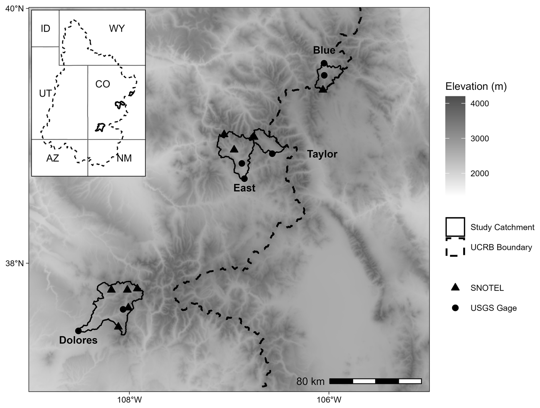
Figure 1 Digital elevation model and geographic context of the headwater catchments included in this study.

2.3 Observation data for model evaluation

We use seven observation data products for model sensitivity and calibration analysis in this study, consisting of both in situ and remotely sensed measurements (Table 1). Daily mean discharge observations were obtained through the USGS National Water Information System dataRetrieval package in R (DeCicco et al., 2024). The locations of USGS stream gauges correspond to downstream points of stream segments in the model. Daily mean in situ SWE and SM were obtained from the NRCS SNOTEL (Snow Telemetry) online report generator. It is common for these observation stations to fall near HRU boundaries (Fig. 1), which likely reduces their representativeness of a homogenous HRU.

Table 1 Observations used in the parameter sensitivity and estimation workflow. Start years are approximate for in situ observations as each station began recording in different years. All outputs from the model area in daily timesteps.

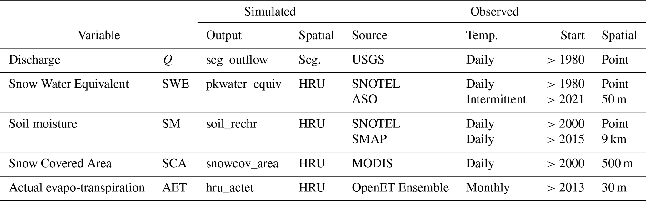
High spatial resolution (50 m) SWE rasters from ASO are derived from airborne LiDAR measurements where the aircraft flies over the catchment of interest (Painter et al., 2016). These acquisitions pertain to specific catchments and are requisitioned by water managers one to several times throughout a water year. The low temporal resolution is unique to this dataset; however, the spatial completeness allows for a more robust estimate of HRU mean SWE compared to SNOTEL point observations. The MODIS snow covered area product used in this study (MOD10A1.061) was used to provide an estimate of fractional snow-covered area (fSCA) and required additional screening and transformations before it could be directly compared to the model output (Sect. S1 in the Supplement). We computed by HRU area averages for ASO SWE and MODIS SCA for direct comparison with model outputs.

The soil moisture observations also required pre-screening and transformations to be suitable for model evaluation (Sect. S2). The soil moisture sensors at NRCS SNOTEL stations are at 2, 8, and 20 cm depths. Of the three in situ depths, the 2 cm depth observation had the best fit to the model and was used in our analysis. The level 4 SMAP product obtained from GEE (SPL4MGP.007) provides measures of saturation at the surface, rootzone, and soil profile at a 9 km spatial resolution, every 3 h from 31 March 2015 to present. Between the SMAP surface and rootzone wetness measurements, the surface zone had the best fit to the model and was used in the final analysis. It is aggregated by HRU and as a daily mean. The model simulates soil moisture storage in a conceptual reservoir, which does not have a physical depth in the soil column. This poses a challenge since it is not directly comparable to observations. Since the simulated and observed values do not match in magnitude, all are normalized between 0 and 1 to compare temporal variability (Hay et al., 2023). We note that there is considerable misalignment between the simulated and observed soil moisture (Fig. S1 in the Supplement), which constrained the identification of behavioral models in this respect.

The OpenET product provides AET at a 30 m resolution using an ensemble mean of multiple satellite based observations and models (Melton et al., 2022). Monthly AET was area-averaged to the HRU scale for comparison with the modeled AET output. The satellite remotely sensed observations (SCA, SMAP, AET) were obtained using Google Earth Engine (GEE) and HRU geometry files from the NHM.

2.4 Selected performance metric

Summarizing a time series of the model's error or behavior into a statistic is a necessary step in model diagnostics and has strong implications for the results of sensitivity analysis and Monte Carlo filtering. Here, we use the normalized root mean squared error (NRMSE). It is calculated by normalizing the root mean squared error by the standard deviation of the observations σ_O, as shown in Eq. (1):

$$\begin{array}{}\text{(1)}& \text{NRMSE}={\displaystyle \frac{\text{RMSE}}{{\mathit{\sigma }}_O}}={\displaystyle \frac{\sqrt{\frac{\mathrm{1}}{T}{\sum }_{t=\mathrm{1}}^T(S_t-O_t{)}^{\mathrm{2}}}}{\sqrt{\frac{\mathrm{1}}{T}{\sum }_{t=\mathrm{1}}^T(O_t-\stackrel{\mathrm{‾}}{O}{)}^{\mathrm{2}}}}}\end{array}$$

where T is the total number of t timesteps in the evaluation, S_t and O_t are simulated and observed values at each timestep, and $\stackrel{\mathrm{‾}}{O}$ is the mean of the observations. This metric allows for comparisons between different catchments and observations because it is not in absolute units, and it accounts for the inherent variability of the location and data. Its value can be interpreted as a proportion: for example, a NRMSE of 0.5 means that the error is half of the variability in the observations. Squared error based metrics suffer limitations such as sensitivity to outliers and errors during high flows (Gupta et al., 2009); however, its interpretability is favorable for comparisons between observations and the rejection of non-behavioral models. NRMSE was used in a recent multi-observational, CONUS-wide NHM calibration study led by the USGS (Hay et al., 2023), and using the same metric makes this work relevant to current agency procedures. For remotely sensed observations, NRMSE is reported as a catchment-wide HRU area-weighted mean, computed over the entire available time series. In the case of ASO, which does not have a time series, NRMSE is reported on a by-acquisition basis.

2.5 Identifying sensitive model parameters using the Morris Method

To identify parameters to be used in the model calibration, we first conduct a type of parameter sensitivity analysis known as screening (Pianosi et al., 2016). This is typically done for models with a large number of calibration parameters (51 in this study) – an important outcome being a reduction in the number of parameters for further analysis. Here, we use the Morris Elementary Effects method, which coarsely samples the parameter space using a one-at-a-time (OAT) approach and is a relatively computationally efficient screening method (Herman et al., 2013b; Morris, 1991; Pianosi et al., 2016). We discuss two sensitivity measures: μ^* to describe the magnitude of parameter sensitivity (Campolongo et al., 2007), and a normalized metric η^* for the screening process (Cuntz et al., 2015). We use 51 trajectories in our sampling design (Cuntz et al., 2015; Gan et al., 2014), and use 1000 bootstrap replicates to identify type I (false positive) and type II (false negative) statistical errors in our screening approach (Sect. S3) (Campolongo and Saltelli, 1997; Saltelli et al., 2007). The Morris sampling algorithm and analysis for calculating sensitivity indices were carried out using the sensitivity package in R (Iooss et al., 2024).

The spatial and temporal variability of the sensitivity measures are also presented in this study. When observations are available, we calculate the sensitivity measures in 3 ways: (1) the full period in which forcings and observations are available, (2) at annual intervals between, and (3) for 10 year moving windows stepped in one year increments. Since discharge observations return a high number of sensitive parameters and have the longest period of record, we limit our scope to these observations for temporal analysis. In terms of spatial analysis, we leverage the spatially distributed remotely sensed observations to assess the influence of HRU attributes on parameter sensitivity based on Spearman Rank correlations.

2.6 Monte Carlo filtering to assess parameter equifinality

Following the identification of informative parameters, we employ a simple uncertainty analysis technique known as Monte-Carlo filtering to evaluate performance and parameter estimation. The method involves choosing an objective function (NRMSE in this case) and setting a threshold for behavioral (“good”) or non-behavioral (“poor”) performance. The parameter space is stochastically sampled with a high number of replicates, and the model is run with each parameter set. Depending on the performance criteria and observation data, usually several parameter sets will return as behavioral. The non-behavioral models are filtered out, and the behavioral simulations are used to assess model parameter value uncertainty (equifinality) and performance relationships (Shafii et al., 2015). In this work we select our behavioral threshold as NRMSE<1.0, where the model error is less than the inherent variability in the observations. This threshold is a common benchmark and is analogous to a Nash–Sutcliffe Efficiency of 0.0, as these two metrics are related (Althoff and Rodrigues, 2021; Manikanta and Vema, 2022; Ritter and Muñoz-Carpena, 2013). To assess how the inclusion of alternative observations affects streamflow calibration, we define multi-objective criteria as joint constraints where the model performance is behavioral with respect to discharge and alternative observations. This criterion leads to relatively few behavioral models for the intersection of discharge and SCA, SMS2, and SMAP – leading us to relax the threshold to an NRMSE of 1.5 for these three alternative datasets only.

Latin Hypercube Sampling (LHS) is a sampling approach commonly applied in sensitivity and uncertainty analysis of complex models with a high number of parameters (Helton and Davis, 2003; Sheikholeslami and Razavi, 2017; Shields and Zhang, 2016). It is a suggested approach for generating parameter sets in Monte Carlo filtering based frameworks so the parameter space is uniformly sampled and equifinality can be assessed (Beven and Freer, 2001). In this study, we use maximinLHS function from the R lhs package (Carnell, 2024), which iteratively solves statistical criteria to maximize the minimum distance between sampling points (Johnson et al., 1990). This method is recognized for producing well-distributed, space-filled samples (Chen et al., 2017; Santner et al., 2018). Following recommendations in existing literature, we use 1000 trajectories per parameter in the LHS design (Pianosi et al., 2016). Due to the higher number of trajectories and computational limitations, the simulation period is reduced to one decade (2013–2022) in this experiment. Since pywatershed contains several non-scalar parameters that are spatially distributed by HRUs, temporally distributed by month, or both, we preserved a priori spatiotemporal distributions from the NHM during the Morris and LHS experiments. We apply the “use the mean” procedure from previous PRMS analysis to address the complexity associated with non-scalar parameters (Hay et al., 2006; Hay and Umemoto, 2007).

3 Results

3.1 Sensitivity analysis

3.1.1 Identifying sensitive parameters for calibration

Using the Morris method with seven different observation datasets, we find that both the number and type of parameters identified as informative are considerably influenced by the target observation (Fig. 2). The 51 parameters are binned into their process representation or “module” in pywatershed (right-hand labels). Several parameters emerge as informative across all observations, particularly in the climate module. These include tmax_allsnow (rain-snow partitioning), tmax_cbh_adj, and tmin_cbh_adj (forcing corrections), which highlight the strong effect of meteorological forcings on multiple model processes. The Jenz-Haize potential evapotranspiration coefficient (jh_coef), which acts as an empirical multiplier for potential evapotranspiration, is highly sensitive for all non-snow related outputs. Two parameters governing groundwater flow, gwflow_coef and soil2gw_max, are only identified by discharge data, and the latter is the only standalone type II error across all observations.

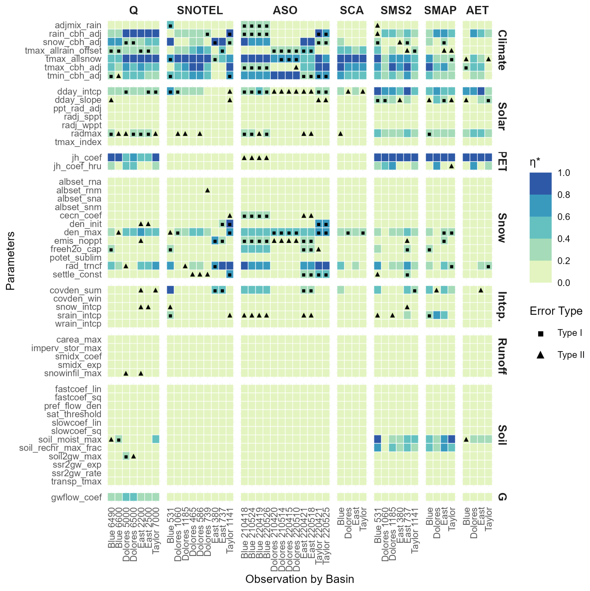
Figure 2 Normalized sensitivity metric η^* for all catchments and target calibration observations available from WY 1982 through 2022. The type I and type II errors are identified via bootstrapping using an uncertainty bound of $\pm \mathrm{1.0}\times SD\left({\mathit{\mu }}_i^{*}\right)$. In the x axis text, the numbers following the catchment name correspond to the last four digits of the USGS gage ID for Q, the NRCS site ID for SNOTEL and SMS2, or the ASO acquisition date in yymmdd format.

The model fit to snow data is sensitive to parameters in the snow module, and as expected in snow-dominated headwaters. Of the four albedo parameters added to our study, none were identified as informative. Simply based on count, discharge observations consistently elicit the largest number of sensitive parameters, with between 10–14 parameters identified among the four catchments (Table S3). The SNOTEL, ASO, and SMS2 observations identify comparable numbers of parameters (10–16), but the precise number of identified parameters varies among catchments. Across all observation datasets, 18–22 informative parameters are identified (22–25 including type II errors). Many of the SNOTEL and ASO parameter identifications have a high number of type I and type II errors, shown by black squares and triangles in Fig. 2. The frequency of these errors suggests that parameter sensitivity with respect to SWE has high variability. This is supported by visualizations of the fitted logistic function, where the error bars for the informative parameters are considerably larger (Figs. S2–S5). While uncertain, the SWE related observations contribute one to six parameters in addition to what is identified by discharge, and the other observations generally contribute relatively fewer unique identifications. While SCA also assesses model performance with respect to snowpack simulation, it returns a consistent, yet, smaller number of identifications and does not exhibit the same extent of statistical errors as the SNOTEL and ASO data.

3.1.2 Parameter sensitivity to annual forcing anomalies

There is considerable interannual variability in the magnitude of parameter sensitivity with some influence of annual temperature and precipitation anomalies. For example, jh_coef was more sensitive in warm, dry conditions than in cold, wet conditions (Fig. 3). We also see differences in the magnitude of sensitivity between catchments, such as rad_trncf being less sensitive in the Dolores compared to the others. Across the four most sensitive parameters, we find relative increased sensitivity in dry conditions (with respect to discharge observations). For this analysis, we use μ^* rather than η^* to assess the overall magnitude of sensitivity.

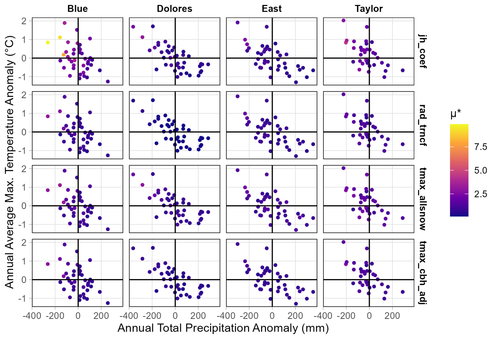
Figure 3 Annual sensitivity measures μ^* for select parameters with respect to discharge observations at the most downstream stream gage point.

Time series analysis of parameter sensitivity illustrates these modest climate sensitivities across all parameters (Figs. S6–S9). On an annual scale, the number of identified parameters ranges from 12 to 17, with the largest variability in snow and interception parameters (Fig. S6). In terms of sensitivity magnitude, the climate, PET, and snow parameter groups show the most variability (Fig. S7). When the sensitivity measures are computed over a 10 year moving window, the screening results are far more stable (Fig. S8). Parameters that are near the screening threshold fluctuate between being identified as sensitive versus not, such as radmax. This is likely due to changes in the most sensitive climate parameters (Fig. S9), since their sensitivity indices are used to produce the normalized metric for screening.

3.1.3 Relationship of geographic attributes and parameter sensitivity

Among the highly sensitive parameters, relationships between HRU attributes and parameter sensitivity range from weak to moderate (Fig. 4). Some correlations among HRU average annual precipitation and μ^* were statistically significant (p<0.05) but with limited explanatory power. The strongest correlation is a negative correlation between rad_trncf (solar radiation transmission through the canopy) and winter maximum temperature (Tmax); rad_trncf is also more sensitive at high elevations and relatively high precipitations. Similarly, jh_coef, tmax_allsnow, and tmax_cbh_adj are each generally more sensitive at higher elevations and cooler temperatures. While jh_coef is less sensitive to snow-related observational data, it shows a similar relationship with the climatic attributes across each observation type. Overall, the magnitude of sensitivity for these select parameters is positively correlated with precipitation and elevation and negatively correlated with temperature. We expect these relationships due to the strong covariance between climate forcings and elevation (Fig. S10), but the differences in explanatory power suggest there are other confounding factors. These results demonstrate that while HRU attributes have relatively low predictability of precise sensitivity measures, the most sensitive parameters are moderately associated with temperature and elevation in particular.

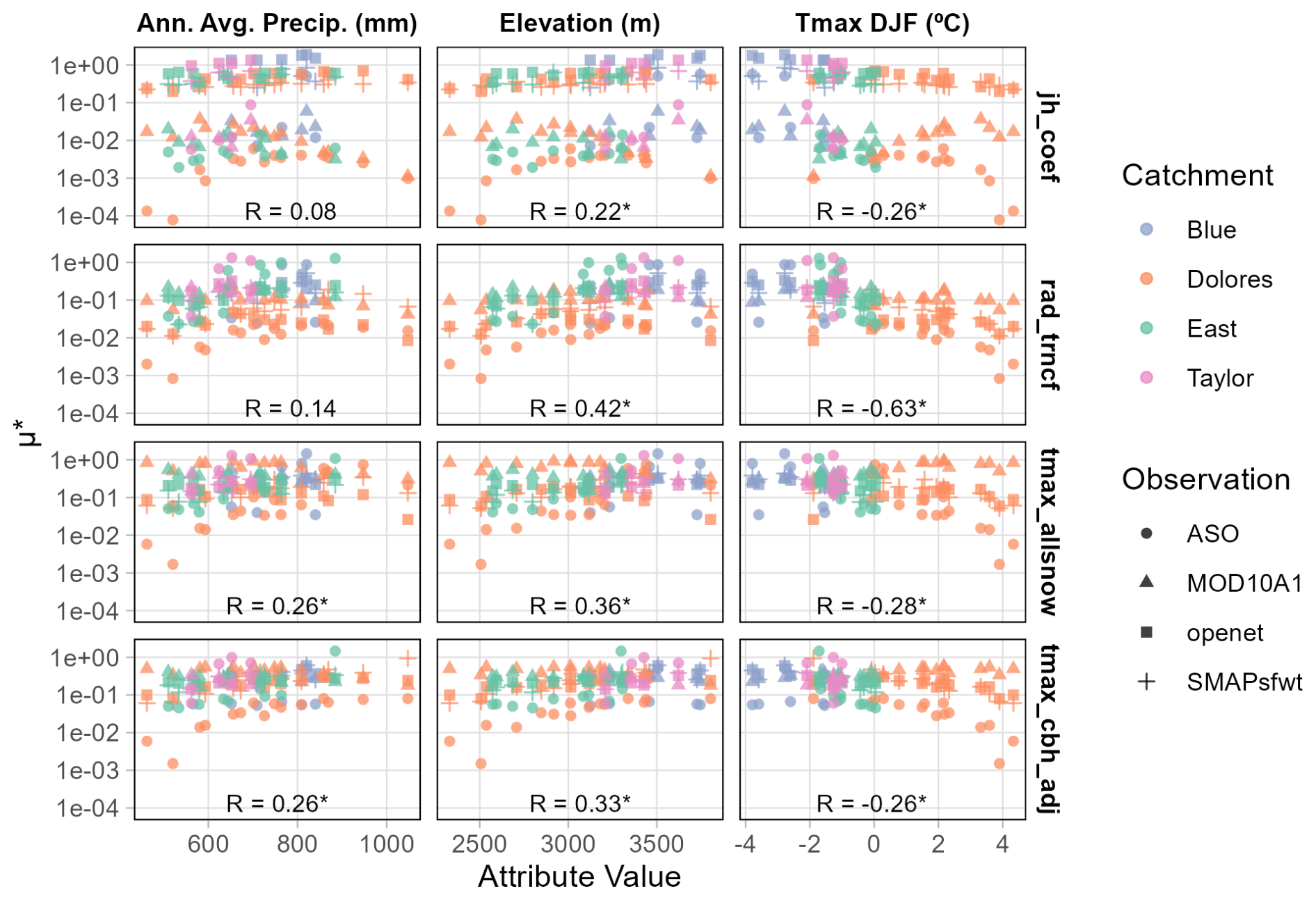
Figure 4 Morris bootstrapped sensitivity metric μ^* for selected parameters versus geographic attributes (annual average precipitation, elevation, and maximum temperature in DJF). Spearman rank correlation values are denoted by R. Statistically significant correlations (p<0.05) are denoted with an asterisk. Each point represents a by-HRU sensitivity measure for a specific observation dataset, catchment, and HRU attribute. The y axis is logged for improved interpretation of the absolute sensitivity measures.

3.2 Monte Carlo filtering calibrations

3.2.1 Constraining equifinality with multiple observations

With NRMSE of daily discharge as the governing objective, we demonstrate how the inclusion of alternative observations can constrain equifinality. Some catchments yield a much higher number of behavioral simulations than others with respect to discharge NRMSE alone (Table 2). For example, out of 22 000 simulations for the Dolores, over 20 % are returned as behavioral, while less than 3 % of 24 000 simulations are returned from the Blue. The Dolores and the East are the larger of the four catchments and return greater proportions of behavioral streamflow simulations, suggesting that model may be more representative over larger scales compared to headwater catchments.

Table 2 Number of behavioral models for where the filtering threshold is set to NRMSE<1.0. The percentage of total simulations is shown in parentheses. Where there are multiple rows, each row denotes a specific in situ observation station or ASO acquisition (in ascending order). The numbers in bold font indicate the greatest overall improvement in NRMSE(Q) of that criterion.

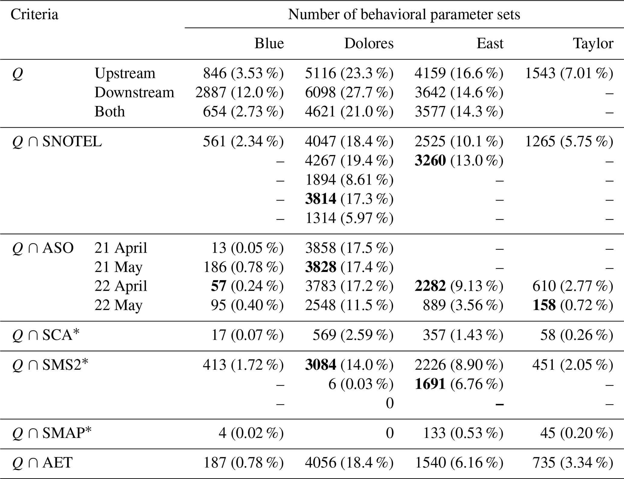
^∗ Denotes where the NRMSE threshold for the alternative observations is 1.5.

Multiple ASO acquisitions show that behavioral SWE simulation is highly dependent on the catchment and date of acquisition. The larger catchments have overall a greater number of behavioral ASO simulations. Results in the Blue suggest that the modeled SWE is less erroneous in May than April. However, the other catchments do not provide a clear indication whether the model better represents April versus May SWE.

While hundreds to thousands of simulations are behavioral for the intersection of Q and SWE, the same filtering threshold (NRMSE<1.0) resulted in zero to a few dozen parameter sets for SCA, SMS2, and SMAP. Instead of discarding the information, we relaxed the threshold to 1.5 for these calibrations to permit further interpretation. Even then, very few behavioral parameter sets are yielded for the soil moisture observations in the Dolores catchment (Table 2). We note that this performance level is within the range of output from the National Hydrologic Model (Table S4). This finding suggests potential issues with model-to-observation alignment. The AET performance was calculated using a monthly mean, which yields behavioral models under the stricter threshold (NRMSE<1.0). This is expected due to the model-to-observation congruency and the suppression of daily variability.

3.2.2 The effect of multiple criteria on streamflow performance

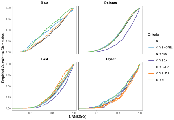
Of the alternative observations used in this study, AET is the only one to consistently improve discharge performance (Fig. 5). The empirical cumulative distribution functions of NRMSE(Q) in Fig. 5 show that the intersection with AET yields a distribution that is better than Q alone (green line is left of the black line in Fig. 5). The observations that induce a worse distribution in discharge performance can be considered misinformative. However, whether these observations improve or reduce discharge performance is dependent on the catchment. For example, ASO shows slight reductions in performance for the Dolores and East (right of the black line in Fig. 5), but some of the best performance in the Blue and Taylor. The latter have fewer behavioral discharge simulations to a begin with – thus, the inherently reduced parameter space may affect how new observations inform the model. The effect of ASO observations on streamflow performance also varies among individual acquisition dates and sites (Figs. S11–S14). Similarly, some SNOTEL locations induce performance improvements while others induce reductions. These results suggest that introducing alternative observations does not always lead to positive streamflow performance outcomes. However, in the case of pywatershed, monthly mean AET observations may be useful in this respect.

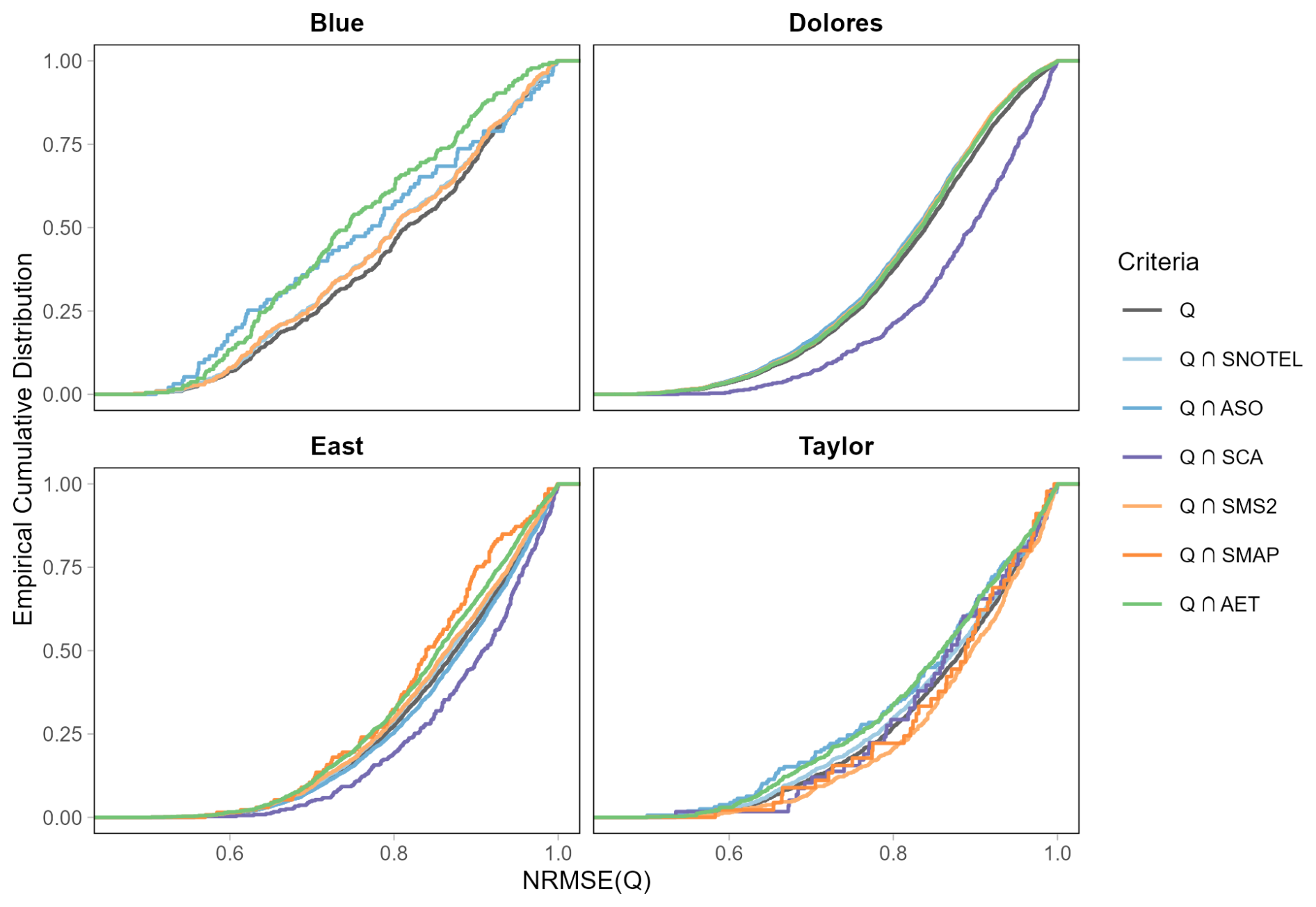
Figure 5 The cumulative distribution of streamflow performance, NRMSE(Q), for different intersections between streamflow and alternative observations. A distribution that is closer to zero (left) is considered informative in the case of NRMSE.

3.2.3 Parameter estimation

The effect of Monte Carlo filtering with alternative observations on behavioral parameter estimation ranges from marginal to pronounced. In most observation and catchment combinations, the parameter values span the entire possible range (Fig. 6). This result alludes to issues with equifinality and the use of prescribed parameter ranges from the PRMS documentation. In only a few cases (such as the use of SMAP for jh_coef estimation in the East River), the introduction of additional observational data reduces the extent of behavioral parameter ranges. Parameter estimates from the three snow-related observations (SNOTEL, ASO, and SCA) show variable agreement. Overall, ASO is relatively consistent among acquisitions (Fig. S15). The highly sensitive potential evapotranspiration parameter jh_coef is generally shifted to a lesser value when intersecting with AET observations

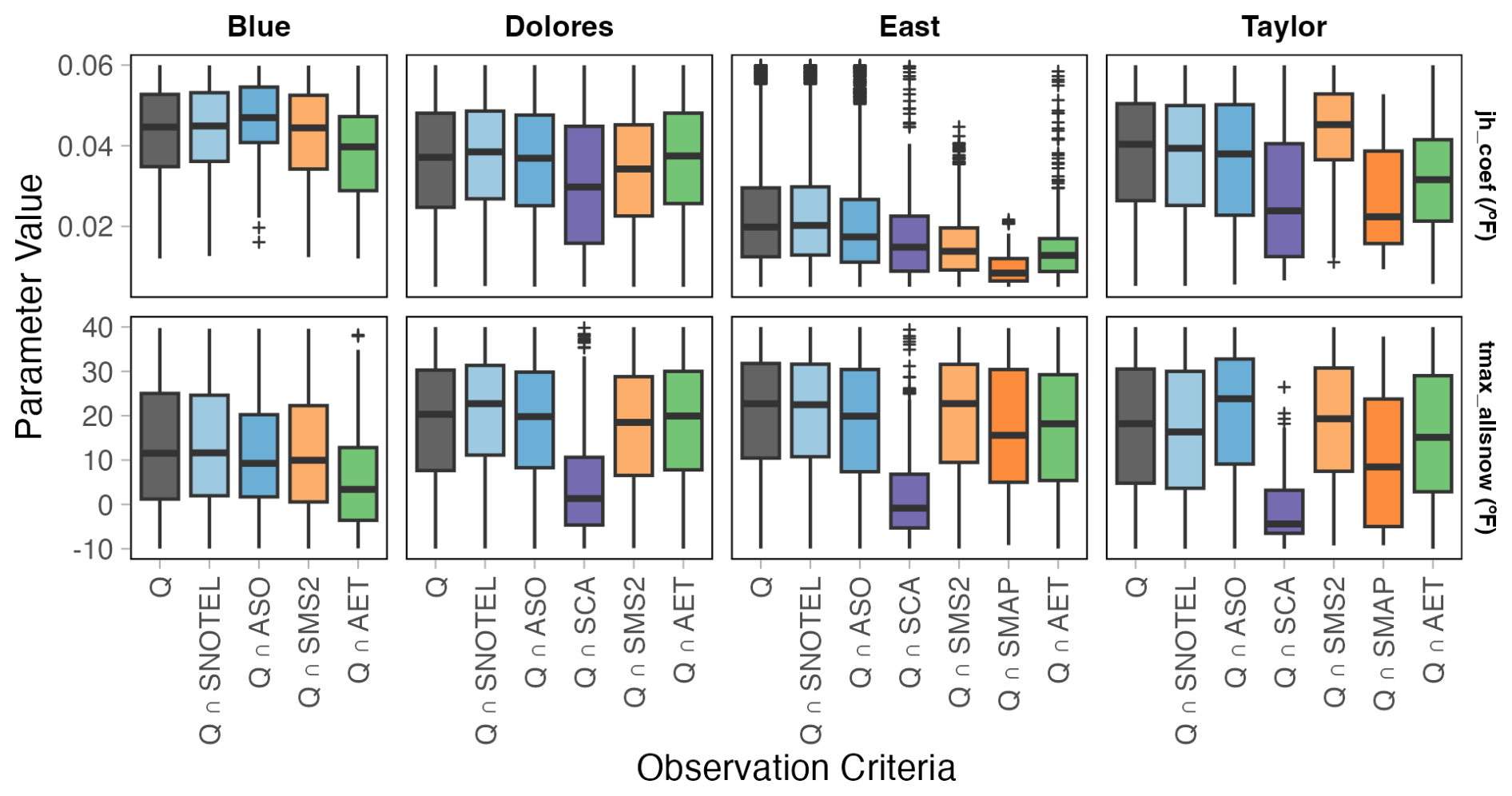
Figure 6 The inter-quartile ranges of behavioral parameter values fluctuate across observation intersection criteria. For catchments that have more than one stream gauge, the behavioral intersection of both stream gauges is used. For SNOTEL, SMS2, and ASO, the best performing site/acquisition is shown. Datasets that returned an insufficient number of behavioral parameter sets are excluded.

4 Discussion

4.1 Model to observation alignment

A core challenge of using additional observational constraints in process based hydrologic modeling is that the simulated variables may not be physically well aligned with what is observed (McCabe et al., 2017). This becomes particularly evident in lumped or semi-lumped models (such as pywatershed) as well as coarsely gridded models (Ehlers et al., 2019; Motovilov et al., 1999), where in-situ point observations are compared to a much larger simulated area. This is the case for SNOTEL SWE and SMS2, and may be a cause of the lack of behavioral parameter sets with respect to SM. In our case study watersheds, these observation points are near topographic high points and therefore are often near catchment or HRU boundaries (Fig. 1). Observation points in these locations are likely not well-aligned with the simulated areal average snowpack or soil moisture over an HRU. We see from the Monte Carlo filtering that streamflow performance can be both hindered and improved by these point-based SWE and SM measurements, but this result is largely dependent on the station (Figs. S10–S13). Where the in-situ observations degraded streamflow performance, we attribute this to poor spatial representation of the HRU.

Aside from the spatial misalignment, the conceptual or physical representations may not fit observed quantities either. In the case of pywatershed, this issue was apparent when comparing simulated and observed soil moisture. The model uses a conceptual framework for soil water storage and fluxes, representing SM storage as a series of conceptual reservoirs. However, in situ measurements of SM are at discrete depths in the soil column. Similarly, satellite remotely sensed soil moisture from SMAP retrieves soil moisture at discrete depth ranges. To address these discrepancies, the model output and observations were normalized between 0 and 1 before comparison, as done in previous work (Hay et al., 2023). Yet, the conceptual misalignment seemed to persist during the Monte Carlo simulation, since the model failed to yield behavioral parameter sets when soil moisture was included in the performance criteria (depending on the catchment, Table 2). Similarly, the baseline parameter sets from the extensively calibrated NHM also perform poorly for soil moisture (Table S4, Fig. A1). This suggests that alternative approaches for addressing the model-to-observation SM alignment may be needed. In Mei et al. (2023) where PRMS was calibrated with SM observations, both the simulated and observed datasets were treated as anomalies, which assesses timing rather than magnitude or variability. Brocca et al. (2014) showed that temporal SM anomalies show lesser spatial variability than absolute magnitude, and other SM calibration studies employ adjustments to in-situ and remotely sensed SM data to remove biases (Draper et al., 2009; Rajib et al., 2016). In another hydrologic calibration with SMAP, temporal correlations were used to assess performance (Koster et al., 2018). In light of the normalization technique used in this study, additional bias corrections or temporal relationships should be explored in future work.

While remotely sensed observation products largely address the point-to-HRU challenges of in situ observations, they are still subject to model-to-observation challenges and uncertainty in the observations themselves. Area averaged ASO SWE, MODIS SCA, and OpenET AET are theoretically well-aligned with the HRU based output of pywatershed. However, uncertainty in remotely sensed data is complex, stemming from the sensors, cloud conditions, surface conditions, spatial sampling, and post-processing (Povey and Grainger, 2015). For example, the ASO SWE product is based on airborne lidar retrievals of snow depth and the snow density is modeled post-hoc, which inherently introduces uncertainty (Painter et al., 2016). The OpenET product is based on satellite optical data, weather data, and an ensemble of models, but yields a single estimate of AET (Melton et al., 2022). The MODIS SCA product and SMAP SM product also yield a singular estimate, which has well documented uncertainties (Liu et al., 2021; Stillinger et al., 2023). Despite the well-known challenges of remotely sensed observations, in this paper they are not explicitly addressed, and we instead opt for “out of the box” implementations.

4.2 On identifying sensitive parameters in headwater catchments

Other PRMS sensitivity analysis studies agree with our overall findings. The most recent and comprehensive sensitivity analysis by Markstrom et al. (2016) encounters similar results: the sensitivity in mountainous headwater catchments is largely driven by a select few parameters. They show that parameters such as jh_coef and tmax_allsnow explain the majority of parameter sensitivity. Other studies with different models also show that rain-snow partitioning and forcing corrections are highly sensitive components in modeled streamflow in mountainous headwaters (Mai et al., 2022; Singh et al., 2024). To the extent that the most sensitive parameters represent corrections of errors in forcing inputs, these results corroborate arguments that forcing input uncertainty is generally greater than model errors (Lundquist et al., 2019). Across two large-scale studies, evapotranspiration emerges as the primary component of model sensitivity, or “dominant process” in the UCRB region (Mai et al., 2022; Markstrom et al., 2016).

In the present study, few, if any, runoff parameters were identified as informative. We posit three reasons for this: (1) that snowmelt has a much greater implication for runoff timing and volume, and (2) that pywatershed has a strong emphasis on forcing data adjustments, and (3) that parameters in other process groups are more impactful to runoff than the runoff parameters themselves. In support of the first line of reasoning, the runoff parameter snowinfil_max is associated with a type II error in the East River (Fig. 2), which suggests the importance of snowmelt. Snowpacks are the primary contributor to runoff volume in high elevation, snow-dominated catchments and rainfall has marginal contributions to runoff volumes (with the exception of rain on snow events) (Hammond and Kampf, 2020; Li et al., 2017). Since squared error based objective functions (NRMSE in this case) strongly penalize errors at high flows (Gupta et al., 2009), where the model inaccurately simulates the timing or magnitude of the spring snowmelt driven streamflow pulse, the parameters driving that inaccuracy would be deemed sensitive. Snowmelt also contributes to seasonal soil moisture regimes in mountainous catchments (Harpold et al., 2015), which could explain why we may not see sensitive runoff parameters for the fit to soil moisture observations either.

Secondly, the forcing adjustment parameters and their ranges from the PRMS documentation influence parameter identification. Complex models with a large number of parameters often exhibit nonlinear sensitivities and strong parameter interactions (Saltelli et al., 2019), and previous work has shown that the selection of parameter ranges impacts the outcomes of sensitivity analysis (Shin et al., 2013). For example, tmax_allsnow has a wide range (Fig. 6) and represents the monthly maximum temperature where precipitation is assumed to be snow (Table S1). Rain to snow partitioning parameters often are constrained within a few degrees of freezing on shorter timescales (Jennings et al., 2018), but this representation in the model makes it more of a tuning parameter with a less clear physical basis. The σ indices yielded from the Morris experiment indicate that this parameter has relatively high nonlinear effects (Fig. S16) – if the range were narrowed, the sensitivity index μ^* would likely change. Since the sensitivity index for screening (η^*) is normalized by the maximum μ^*, this has implications for which parameters are identified as informative. Additionally, the Morris method may not provide as reliable of indices for highly sensitive parameters when compared to quantitative methods, such as Sobol (Herman et al., 2013b; Sobol', 2001). However, in the context of model calibration and parameter estimation, it is important to prescribe parameter ranges that cover the optimal space while remaining efficient (Bárdossy and Singh, 2008; Mai, 2023). The effects of a priori parameter ranges are not addressed in this study, but could be assessed in future work.

It is plausible that the high sensitivity/reliance on forcing adjustments could mask structural deficiencies in the model's snowmelt and runoff generation mechanisms. In that case, we would expect the parameter values to exhibit concentration at the bounds, pronounced shifts when SWE constraints are introduced, or dramatic shifts across similar catchments. Instead, we see that the inter-quartile ranges are similar between catchments and calibration criteria, and that the range of acceptable values is wide. This signals substantial equifinality, rather than compensation for structural bias. The similarities between the discharge-only and discharge + SWE criteria suggest that most of the information about the parameter value is embedded in the discharge signal. We acknowledge that structural uncertainty cannot be assessed without testing additional model formulations; however, the current evidence does not suggest that these forcing correction parameters mask deficiencies in the snowmelt or runoff mechanisms.

For the third reason, we find parameters outside of the runoff module, such as soil_moist_max and gwflow_coef are more identifiable with respect to discharge than parameters within the runoff module itself. Other studies have arrived at similar conclusions, noting that the runoff process requires the largest number of parameters to explain 90 % of it's sensitivity, while other processes only rely on a few (Markstrom et al., 2016). Parameters within other process groups, such as soil and PET, explain runoff sensitivity in a greater proportion of CONUS than runoff parameters like smidx_coef and smidx_exp (Markstrom et al., 2016). Since soil_moist_max and gwflow_coef represent processes relevant to catchment geology, like infiltration and groundwater flow velocity (Table S1), this finding is logically coherent and supported by previous work.

We clarify that the objective of this work is to assess the impact of observational data selection on parameter identifiability, rather than conventional sensitivity analysis. This distinction is made by Gupta and Razavi (2018), where an identifiability analysis focuses on model sensitivity with respect to observations (by using an objective function) versus sensitivity to the output itself. These methods are fundamentally distinct from each other. Choosing an objective function to summarize the model responses limits the interpretation of process importance because the “sensitivity” is influenced by how well the model tracks observations. Given that the choice of objective function has a pronounced impact on how model residuals are penalized, it therefore influences what parameters are considered informative. Our approach therefore cannot support the identification of dominant processes; however, it holds utility in parameter screening with the aim of calibrating a model to a suite of observations (Pianosi et al., 2016).

4.3 Model selection impacts on sensitivity and uncertainty analysis

We sought to explore some of the numerous choices that a modeler faces during a calibration experiment. The primary focus of this study was on the choice of calibration target data, as well as simulation period and catchment. Other important choices include the model itself, the calibration algorithm, forcing inputs, and the objective function. These choices were controlled for in our study by using a single model, a uniform sampling LHS design, one forcing dataset, and a grounded objective function threshold. A vast body of work discusses the nuances in inter-model comparison (Mendoza et al., 2015), advancement of calibration techniques (Mai, 2023), the uncertainty in forcing inputs (Tang et al., 2023), and the implications of objective function choice (Lamontagne et al., 2020). While there are limitations to using a single objective function for model evaluation (Clark et al., 2021; Legates and McCabe, 1999), for simplicity and scope we find NRMSE to be appropriate for a multi-observation framework (Gupta et al., 2008, 2009). There is also subjectivity in the design of the Morris and LHS experiments (Gan et al., 2014); we made these choices by following recommended values for discretization levels, trajectories, and rejection criteria (Cuntz et al., 2015; Pianosi et al., 2016).

Previous works have found that multi-observational calibration leads to better representation of hydrologic process and improved streamflow simulations (Finger et al., 2015; Smyth et al., 2020; Wongchuig et al., 2024; Zhou et al., 2020). Other multi-observational PRMS based studies have found that AET and soil moisture can improve streamflow performance (Mei et al., 2023). Our results only partially support this notion. While these findings are promising, a recent review poses the question “Increasing amount of collected data: to use or not to use?” (Herrera et al., 2022). We provide a conflicting answer to this question, as some observations constrained behavioral simulations into worse performing areas. One prior study found that the inclusion of ASO has positive implications for streamflow prediction in one California catchment with a large number of acquisitions (Lahmers et al., 2022). Our results agree with this finding in the Blue and Taylor but disagree in the Dolores and East.

We suggest a few possible reasons for the instances of poorer distributions of model performance: first, simulations that fail to adequately simulate intermediate state variables (such as SWE, SM, or AET) may have had structural compensating errors that ultimately yield good streamflow performance, even if for the wrong reasons. For example, high precipitation biases could be compensated for by high soil moisture storage when soil moisture is not used as a calibration target, but these simulations would be removed when soil moisture observations are included. Second, the approach to the multi-objective problem influences the way equifinality is assessed. Our use of joint constraints is clear cut, demanding that performance criteria is met for more than one set of observations. However, there are numerous alternative approaches, such as adaptive data assimilation techniques (Liu et al., 2012), pareto optimization (Madsen, 2003), or informal Bayesian methods (Choi and Beven, 2007). Each approach is unique in its integration of alternative observations and assessment of parameter uncertainty/equifinality. Our logical framework inherently reduces the equifinal space as more observational constraints are introduced, but pareto optimization or fuzzy logical constraints may expand it. Lastly, the model-to-observation alignment as discussed in Sect. 4.1 plays a significant role in constraining parameter values.

Additionally, the modeler must make decisions on the spatial and temporal resolution for model evaluation. While streamflow observations are commonly used in daily timesteps, the modeler may consider using monthly or annual averages to assess performance (Hay et al., 2023). Notably, the OpenET dataset from Google Earth Engine is only available as monthly averages and was identified as the most informative alternative observation dataset in this study. Future work should include the use of different temporal resolutions in model evaluation. Errors at daily timesteps may result in harsh penalization, while longer term trends could be adequately represented. However, previous work has noted that models calibrated to monthly streamflow yield unrealistic daily values while models calibrated to daily data (Adla et al., 2019) and others have highlighted the relationships between model complexity, process timescale, and the spatial and temporal resolution of calibration data (Kavetski et al., 2011). We hypothesize that parameter estimation for daily streamflow is constrained beneficially by monthly AET because it provides more holistic information about the catchment water balance, but the examination of this hypothesis warrants further work and is not currently possible with OpenET.

In a similar vein, results from sensitivity analysis depend in part on the calibration period and window size (Herman et al., 2013a; Massmann et al., 2014; van Werkhoven et al., 2008). Previous literature notes that sensitivity measures become stable for five year windows or greater, muting the effects of interannual variability (Shin et al., 2013). Our assessment of streamflow over multiple 10 year rolling windows (Figs. S8 and S9) corroborates this finding. However, the user must be cautious of type II errors, as they arise for parameters that straddle the identifiability threshold in the Morris experiment (Figs. S2–S5). We continue the recommendation of bootstrapping the elementary effects to identify these errors (Campolongo and Saltelli, 1997).

4.4 Implications for water resource operations and forecasting

The parameter identification and estimation results presented in this study help inform operational modeling practices and could be extended to forecasting frameworks. Multi-observational modelling techniques have been a subject of increasing attention in the last decade (Liu et al., 2012) and are a promising tool for the improvement of ensemble forecasting (Troin et al., 2021). However, our results suggest that the integration of alternative observations has spatially heterogenous implications to streamflow performance, despite the four case study catchments being within a similar geographic region. In the adjacent East and Taylor River catchments, we see that the augmentation of streamflow performance for each dataset is different (Figs. 5, S12, and S13). This may result from uncertainty in the model, since the smaller headwater catchments yielded fewer behavioral parameter sets in the Monte Carlo Filtering step (Table 2). These differences between catchments could also be explained by differences in hydroclimatic variables, such as runoff ratio or aridity (Elkouk et al., 2024; van Werkhoven et al., 2008). We find that runoff ratio and aridity are similar across the catchments in this study; however, we note a 7 % difference in runoff ratio between the East and Taylor catchment, which may affect the differences we observe in streamflow performance when including soil moisture data (Table S2). At broader scales, the simulation of streamflow would likely be improved by different datasets, as the dominant hydrologic processes vary by ecologic and physiographic characteristics (Mai et al., 2022; Markstrom et al., 2016). The methods used in this study, Morris screening and LHS Monte-Carlo filtering, are relatively straightforward analytical techniques that were completed on a laptop computer. Future work to accomplish this assessment at broader scales in a computationally parsimonious way would be valuable.

5 Conclusions

A multi-observation sensitivity and uncertainty analysis of the pywatershed hydrologic model is presented in this study. In four headwater catchments in the UCRB, we obtained seven observation datasets pertaining to discharge, snow water equivalent, snow-covered area, soil moisture, and evapotranspiration to use as objective targets in a Morris parameter screening and Monte-Carlo filtering analysis. Results show that the use of alternative observations allows for the identification of more informative parameters in the screening analysis. The outcomes of streamflow performance and parameter estimation vary considerably across catchments and observation data criterion.

Starting with 51 model parameters, the Morris screening method identifies nearly twice as many informative parameters when including alternative observations versus discharge alone. Bootstrapping of the sensitivity metrics allows for the identification of type I and type II statistical errors, which avoids the exclusion of parameters that have sensitivities near the identification threshold. Across the four catchments, forcing corrections and rain-snow partitioning parameters have a high impact on the model fit to observations. The identification of informative parameters is highly variable over annual timescales, but over decadal timescales it is relatively stable due to the suppression of interannual variability. Spearman rank correlations between parameter sensitivity and catchment attributes such as precipitation, temperature, and elevation are weak to moderate.

With the informative parameters carried into the maximin LHS Monte-Carlo filtering analysis, we find that multi-observation criteria considerably reduce equifinality. However, by reducing the number of acceptable parameter sets, streamflow performance may be either positively or negatively constrained. Our results suggest that AET is consistently useful for the improvement of streamflow simulations in UCRB catchments, but the value of other alternative datasets needs to be assessed on a case-by-case basis. Snow and soil moisture datasets yield both increased and decreased performance depending on the catchments. Additionally, the observation criterion has strong impacts on the range of estimated parameter values

The use of alternative observations is found to be informative in parameter screening but has uncertain and spatially heterogenous outcomes in terms of streamflow performance and parameter estimation. We note that observation quality and model-to-observation alignment are important aspects of the analytical framework used in this study. Given the nuance of observations such as SMAP, ASO, and OpenET, these findings may be considered in future work where multi-objective calibration is of interest.