An argument for parsimony in differentiable hydrologic models

Differentiable hydrologic models that use machine learning to infer parameters for process-based models show promise for both prediction and inference. However, these models are often developed with time-varying parameters, despite evidence that such flexibility can undermine physical consistency and yield only marginal predictive improvements over simpler static approaches. In this study, we revisit the comparison between static and dynamic differentiable models across 531 CAMELS-US basins, evaluating key architectural choices: (1) neural network type (multi-layer perceptron (MLP) vs. long short-term memory network (LSTM)); (2) process model configuration (single- versus ensemble-parameter estimation); and (3) comprehensive versus alternative input feature sets. Using the Hydrologiska Byråns Vattenbalansavdelning (HBV) conceptual model, we find that although ensemble parameterizations improve performance relative to single-parameter configurations, they also alter the conclusions about the relative value of network architecture: LSTMs outperform MLPs in single-parameter configurations, but static, MLP-based ensembles achieve performance comparable to dynamic, LSTM-based ensembles despite their simpler structure. Additionally, we find that LSTM-estimated parameters rarely exhibit meaningful temporal variability despite their time-varying inputs, and when they do, this temporal variability may reflect hydrologic model equifinality rather than process dynamics. We further show that models using only latitude and longitude as static inputs achieve spatial generalization comparable to models using comprehensive feature sets describing climate, topography, geology, soils, and land cover. Similarly, temporal generalization is retained even when comprehensive features are replaced with physically meaningless values. These results raise the possibility that static inputs may function less as direct representations of physical basin processes and more as spatial proxies for generalization in space or as site identifiers when generalizing in time. Overall, our results support reduced complexity in differentiable hydrologic modeling to provide greater transparency while retaining predictive performance.

1 Introduction

Hydrological models that simulate water fluxes and stores across the landscape are central to water resources management, infrastructure design, flood forecasting, and reservoir operations (Todini, 2007; Wagener et al., 2001). Process-based models have traditionally underpinned these applications, but machine learning models have recently surpassed them in predictive performance (Nearing et al., 2021). In particular, Long Short-Term Memory (LSTM) networks (Hochreiter and Schmidhuber, 1997) have proven highly effective due to their ability to represent long temporal dependencies and are often considered state-of-the-art for catchment-scale streamflow simulation (Feng et al., 2020; Kratzert et al., 2018). Despite their predictive skill, the black-box nature of LSTMs and their lack of physical constraints raise concerns regarding their reliability for extrapolation tasks, such as extreme event prediction and climate change projections (Natel de Moura et al., 2022; Poudel et al., 2026; Razavi, 2021; Reichert et al., 2024; Wi and Steinschneider, 2022, 2024). These concerns are further compounded by saturation limits inherent to such models (Acuña Espinoza et al., 2025; Baste et al., 2025; Kratzert et al., 2024). Consequently, hybrid approaches that integrate machine learning with process-based structure offer a promising pathway to retain predictive gains while preserving physical consistency (Bennett and Nijssen, 2021; Kraft et al., 2022; Reichstein et al., 2019; Shen et al., 2023).

Differentiable models represent a prominent hybrid approach in which neural networks learn parameters of process-based models within a unified, end-to-end training framework. These models can learn regionally coherent process-based model parameters (Shen et al., 2023; Tsai et al., 2021) and have achieved predictive performance comparable to LSTMs in both gauged and ungauged basins (Feng et al., 2022, 2023). The most common differentiable architecture couples an LSTM with a lumped conceptual model, using the network to estimate either a single parameter set or an ensemble of parameter sets (Acuña Espinoza et al., 2025; Feng et al., 2022, 2023; Mangukiya and Sharma, 2025; Zhong et al., 2023). In the ensemble configuration, a single neural network produces multiple parameter sets, each of which is processed in parallel through the process-based model to generate ensemble predictions; the mean of these predictions is commonly used as the final output. Depending on the network design and input features, these parameters may be inferred as static in time or allowed to vary dynamically at each simulation step.

Dynamic parameterizations provide additional flexibility and can yield modest performance improvements in many basins, but their advantages over simpler static formulations remain unclear. Empirical evidence suggests that gains are often marginal (median NSE of 0.732 versus 0.714 in CAMELS-US; Feng et al., 2022) and that dynamic models can underperform static alternatives in certain hydroclimatic regimes, such as arid regions (Feng et al., 2024). From an interpretability perspective, static parameterizations are preferable because they yield a single, basin-specific parameter set that is directly comparable to conventional process-based models. Moreover, several studies caution that dynamically parameterized differentiable models may effectively function as LSTM variants despite their apparent physical structure, thereby inheriting many of the same limitations (Acuña Espinoza et al., 2024; Feng et al., 2022; Acuña Espinoza et al., 2025).

In earlier work, Feng et al. (2022) hypothesized that overuse of dynamic parameterization risks compromising physical consistency for incremental performance gains. More recently, Acuña Espinoza et al. (2024) rigorously tested this by comparing three conceptual model structures coupled with LSTM-based dynamic parameterization: (a) a standard multi-reservoir structure with realistic processes, (b) a single-bucket structure conserving only mass, and (c) a nonsensical structure with implausible processes. They found that all three hybrid configurations achieved performance comparable to a pure LSTM, suggesting that LSTM-based dynamic parameterization can compensate for missing or even implausible physical structural representation, providing the right answer for the wrong reasons (Kirchner, 2006). Nevertheless, dynamic differentiable models dominate the current literature (Bohl et al., 2026; Ji et al., 2025; Mangukiya and Sharma, 2025; Zhong et al., 2023, 2024), while static approaches remain comparatively underexplored.

Interpretations of architectural trade-offs in differentiable modeling are further confounded by conceptual ambiguity in how the literature characterizes LSTM-based estimation of static and dynamic process-model parameters. Previous work has argued that LSTMs can provide both static and dynamic parameterization to process-based models. However, LSTMs are fundamentally dynamic models that operate in two modes: (a) sequence-to-sequence, processing an input sequence to produce an output at each time step, and (b) sequence-to-one, processing an input sequence to produce a single output for the final time step. In the differentiable modeling literature, these modes have been applied in three distinct ways. First, fully dynamic parameterization uses sequence-to-sequence LSTMs to vary all parameters at each simulation time step of the process-based model. Second, “static” parameterization uses sequence-to-one LSTMs to produce parameters that vary between sequences during training, while during testing, the full input for a basin is supplied as a single sequence to get a single parameter set. Third, hybrid parameterization uses sequence-to-sequence LSTMs to vary selected parameters at each time step while treating others as “static”, similar to the second approach.

Critically, although the literature labels parameters as static in the second and third approaches, the LSTMs are actually learning parameters that vary across input sequences. A more appropriate architecture for truly static parameterization would be a Multi-Layer Perceptron (MLP), which takes static basin attributes as input and produces a single basin-specific parameter set, analogous to conventional process-based hydrological models. Despite this distinction, differentiable model comparisons have focused almost exclusively on LSTM formulations, leaving MLP-based static parameterization largely unexplored. MLP-based approaches have been tested in river routing models (Bindas et al., 2024), but their use in rainfall-runoff modelling has so far been limited to hybrid parameterization schemes motivated primarily by the need to reduce computational burden in large-scale, high-resolution modelling efforts, rather than by an explicit assessment of their predictive or interpretive value relative to LSTMs (Song et al., 2025). Similarly, while sequence-to-sequence LSTMs have been criticized for violating physical constraints of process-based models (Acuña Espinoza et al., 2024, 2025), sequence-to-one formulations have received comparatively little scrutiny.

Another argument for LSTM-based differentiable models is that they process time-varying inputs including precipitation and temperature to produce time-varying parameters, with parameter variability presumably indicative of seasonally varying hydrological processes. However, varying parameter sets are not necessarily representative of process dynamics but can merely arise due to equifinality (Beven, 2006), where multiple parameter sets produce comparable model performance. Thus, an alternative interpretation is that LSTMs are capturing equifinality manifesting as cyclical parameter changes through time, rather than meaningful seasonal dynamics. There is some evidence that supports the seasonal dynamics interpretation for sequence-to-sequence LSTMs. Feng et al. (2022) found that a time-varying runoff factor parameter followed a seasonal cycle mimicking basin water storage, which they hypothesized improved streamflow predictions by linking deep groundwater storage to runoff generation. However, whether temporal parameter variability in sequence-to-one LSTMs similarly represents seasonal process dynamics remains unclear.

Input feature selection represents another, closely related challenge in differentiable model development. The neural networks used for parameter estimation are flexible and can ingest many features. As a result, differentiable hydrological models commonly adopt extensive sets of basin attributes – spanning meteorology, topography, geology, land cover, and soils – largely inherited from pure LSTM modeling frameworks (Feng et al., 2022; Kratzert et al., 2018). Recent work, however, questions whether neural networks meaningfully exploit such physical attributes for generalization (Heudorfer et al., 2024, 2025). Heudorfer et al. (2025) compared LSTMs provided with dynamic forcings and static attributes to ablated variants without attributes, finding that while static features improve temporal generalization, they contribute little to spatial generalization, which is primarily driven by meteorological forcings. Should similar limitations apply to parameter learning in differentiable models, extensive static inputs may only promote overfitting to training data without improving generalization.

Motivated by these knowledge gaps, this study contributes a systematic comparison of static and dynamic differentiable models, with focus on sequence-to-one LSTM formulations that have received less scrutiny than their sequence-to-sequence counterparts. We develop differentiable models for CAMELS-US (Addor et al., 2017) basins and evaluate their performance in gauged and ungauged settings based on choices in neural network architecture (MLP versus LSTM), process-based model configuration (single versus ensemble parameter sets), and input requirements (comprehensive versus alternative). We further investigate the temporal variability of LSTM-produced parameters, evaluate their value for prediction, and assess the contribution of dynamic inputs towards parameter learning. Collectively, these analyses are designed to address the following research questions:

1. How do neural network architecture (MLP versus LSTM) and process model configuration (single versus ensemble parameter sets) affect differentiable model performance in out-of-sample evaluations for both gauged and ungauged basins?

2. What static basin attributes are necessary for robust and transferable parameter learning in differentiable models, and how does performance change when using comprehensive versus alternative static inputs?

3. To what extent do dynamic inputs meaningfully contribute to parameter learning or predictive skill in differentiable hydrologic models?

2 Data and Methods

This work compares multiple differentiable model architectures, investigating single and ensemble configurations combined with either MLP or LSTM networks for parameter learning. We also evaluate performance when the networks use comprehensive and alternative static feature sets to determine the necessary inputs for effective parameter learning. Finally, for the LSTM-based differentiable models, we examine the nature of learned process-model parameters and assess how dynamic input features contribute to their estimation. These experiments are described in more detail below.

2.1 Study Area and Data

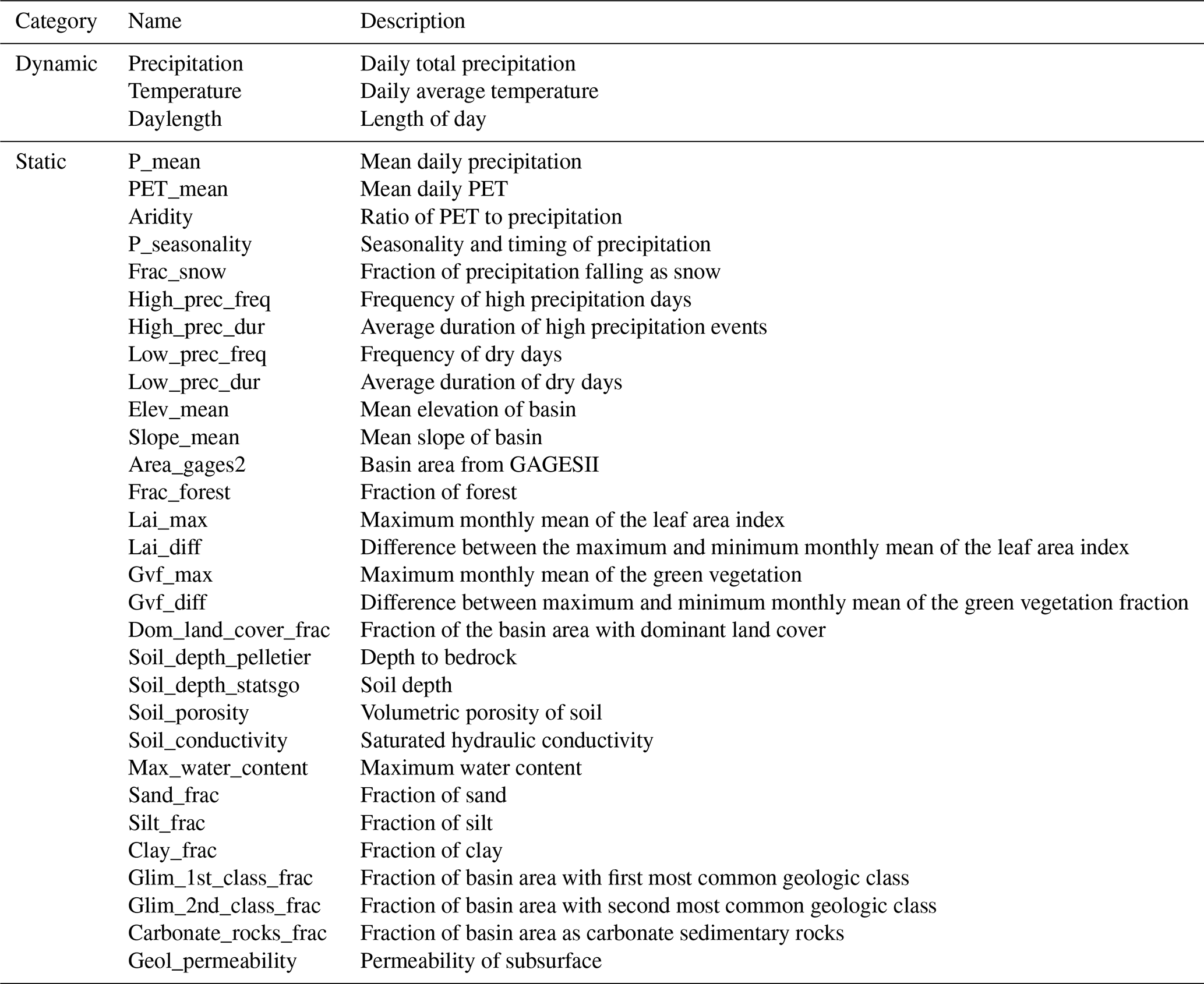
This study examines 531 basins from the CAMELS-US dataset (Fig. A1), filtered by Newman et al. (2017) based on basin size and catchment area reliability. The dataset contains a large set of static input features, spanning meteorology, topography, geology, land cover, and soils data (see Table 1). Daily dynamic inputs are taken from the Daymet meteorological product between 1980–2014, and daily USGS streamflow for each basin is available for the same period.

For all experiments, we randomly hold out 20 % of basins for spatial (ungauged basin) evaluation (see Fig. A1). For the remaining 80 % of basins, we use 16 years (1990–2005) for model training, 8 years (2006–2014) for validation, and 10 years (1980–1989) for testing.

Table 1 Full set of input features used by MLP and LSTM models in differentiable architecture. Dynamic features are only used by the LSTM.

2.2 Process-based hydrological model

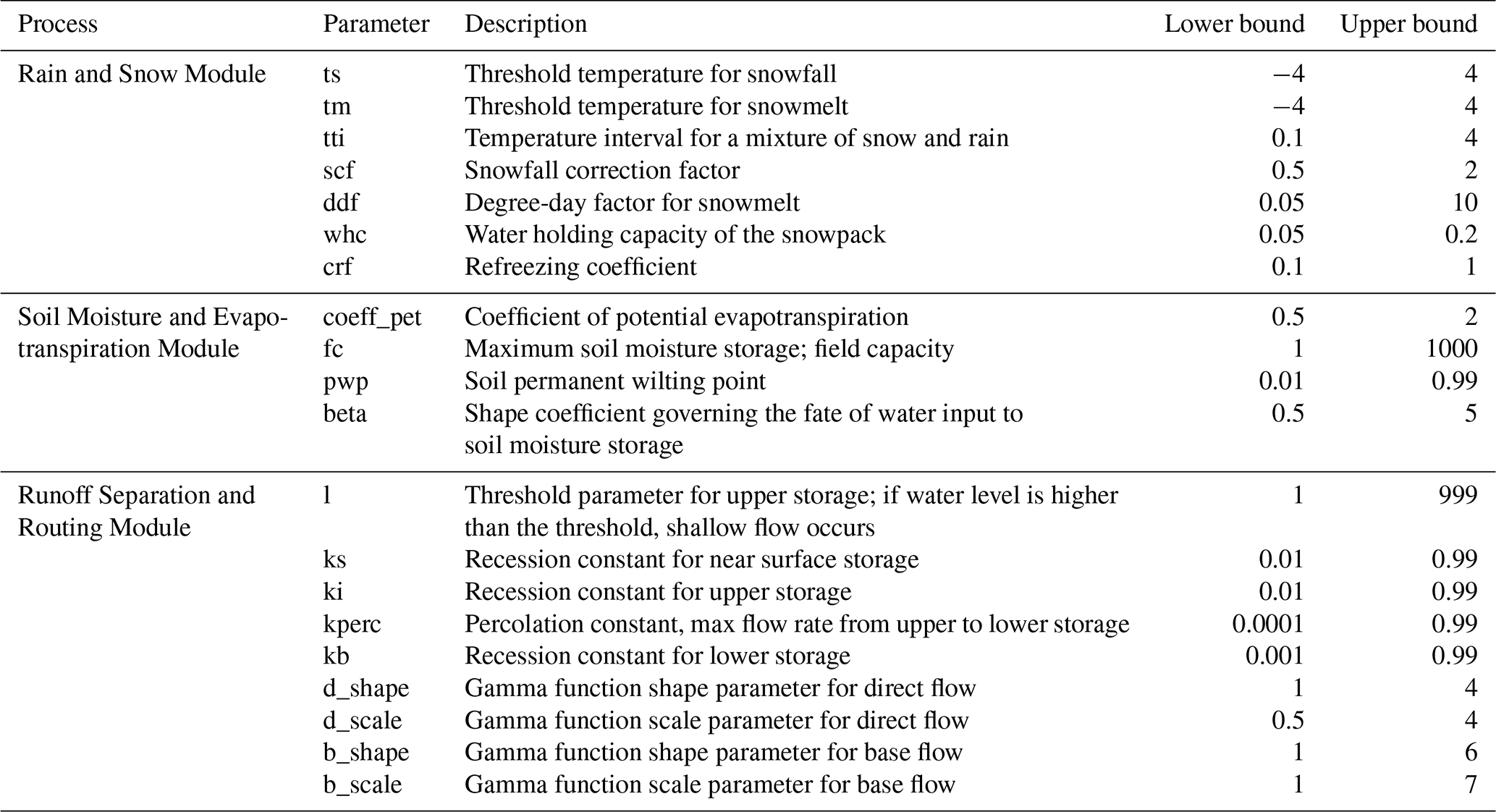
We use the Hydrologiska Byråns Vattenbalansavdelning (HBV) model (Bergström, 1995; Seibert, 2005) as the process-based hydrological model throughout this work. HBV represents watershed processes through 20 parameters distributed across three interconnected modules: snow accumulation and melt, soil moisture and evapotranspiration, and streamflow generation and routing. The model first partitions precipitation into rainfall and snowfall based on temperature thresholds, with snowmelt calculated using a degree-day method. In the soil and evapotranspiration module, actual evapotranspiration is calculated from potential evapotranspiration and available soil moisture. Excess water beyond the soil's storage capacity enters linear reservoirs representing quick flow, delayed subsurface flow, and groundwater discharge. These flow components are aggregated and routed to the catchment outlet through a gamma unit hydrograph function. HBV takes daily series of total precipitation and average temperature as inputs and uses daylength to calculate potential evapotranspiration based on the Hamon method (Hamon, 1961). Additional details on model parameters and process representations are provided in Appendix B (Table B1).

2.3 Differentiable model architectures

Differentiable hydrologic models are developed in a unified, end-to-end framework. A neural network processes static and/or dynamic features to infer parameters of the HBV model, which then uses these parameters together with meteorological forcings to simulate streamflow. Neural network inputs are standardized to zero mean and unit variance, whereas HBV inputs are provided in their original units (mm d⁻¹ for precipitation, °C for temperature).

We consider four differentiable architectures: MLP with a single HBV unit (MLP + HBV), MLP with a 16-unit HBV ensemble (MLP + 16HBV), LSTM with a single HBV unit (LSTM + HBV), and LSTM with a 16-unit HBV ensemble (LSTM + 16HBV). The ensemble size of 16 follows recommendations from prior work (Feng et al., 2022). These configurations are described below.

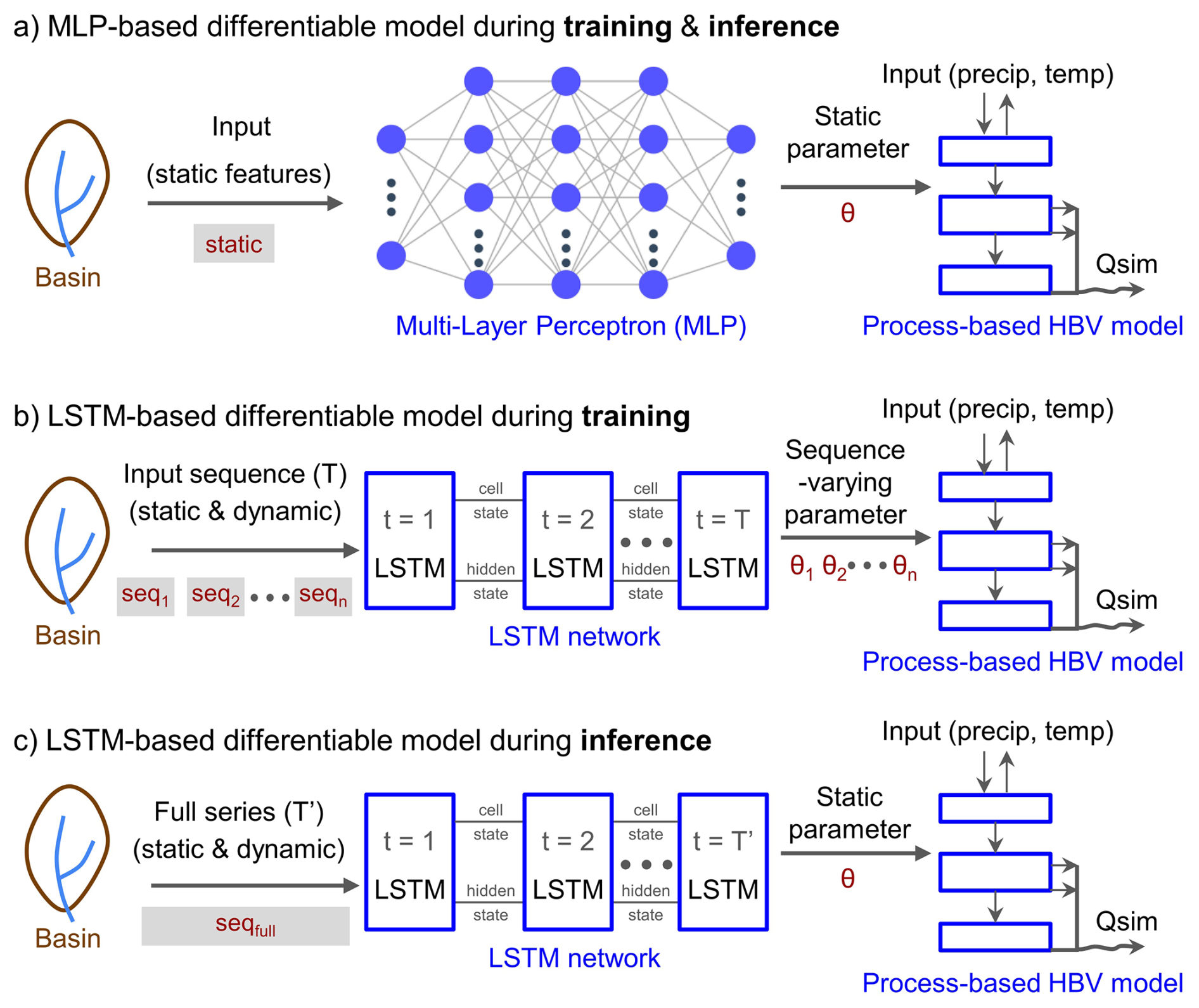
Figure 1 Schematic of differentiable model architecture. (a) MLP + HBV: Static basin attributes are passed through an MLP network to generate static HBV parameters (θ), which are then used by the HBV model to simulate streamflow. This process is identical for training and inference/testing. (b) LSTM + HBV during training: Sequences of concatenated static and dynamic features are processed through the LSTM, with the final hidden state producing HBV parameters for streamflow simulation. Multiple input sequences (seq₁, seq₂, …, seq_n) per basin result in sequence-varying parameters (θ₁, θ₂, …, θ_n) during training. (c) LSTM + HBV during inference: The entire available time series for a basin (seq_full) is processed as one continuous sequence, with the final hidden state producing a single set of static HBV parameters (θ) for streamflow simulation. In all cases, the HBV model receives precipitation and temperature as forcing inputs. The schematic illustrates for a single basin, though models are trained regionally across all basins.

2.3.1 MLP + HBV and MLP + 16HBV

The first network architecture considered is a Multi-Layer Perceptron (MLP), a feedforward neural network composed of multiple fully connected layers that transform inputs through successive nonlinear activation functions. In the MLP + HBV architecture (Fig. 1a), the MLP takes 30 static basin attributes as input – including measures of climate, topography, geology, land cover, and soil type (see Table 1) – and outputs a single vector of HBV parameters per basin. The MLP uses ReLU activations in all hidden layers and a linear activation in the output layer. The resulting outputs are then normalized between [0,1] using sigmoid activation and scaled to parameter-specific minimum and maximum ranges for the HBV model (Table B1).

Each training instance consists of a 3-year sequence of daily precipitation and temperature forcings (ℝ^1095×2) for the HBV model, along with a standardized vector of static basin attributes (ℝ³⁰) for the MLP. The static attributes are first passed through the MLP to produce a single set of 20 HBV parameters (ℝ²⁰). These parameters, together with the 3-year forcing sequence, are then passed to the HBV model to simulate streamflow over the full 3-year period (ℝ¹⁰⁹⁵). The first 2 years of streamflow simulation are discarded for spin-up, and the loss is computed using only the final year. Gradients of the loss are then backpropagated through the HBV model to update MLP weights.

During inference, each basin's static attribute set (ℝ³⁰) and the complete precipitation and temperature forcing record are provided to the hybrid model in a single forward pass. For example, given 15 years (5475 d) of forcing data for a basin, the static attributes are first passed through the MLP to obtain a fixed set of HBV parameters (ℝ²⁰), which are then used together with the entire forcing sequence (ℝ^5475×2) in the HBV model to simulate streamflow for the entire period.

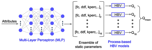
We also consider an ensemble architecture called MLP + 16HBV, which is identical to MLP + HBV except that the MLP outputs an ensemble of 16 parameter sets (ℝ³²⁰). Each parameter set is run through independent HBV units that receive the same meteorological forcings, producing 16 parallel streamflow predictions at each timestep. These ensemble members are averaged to produce the final streamflow prediction (Fig. 2).

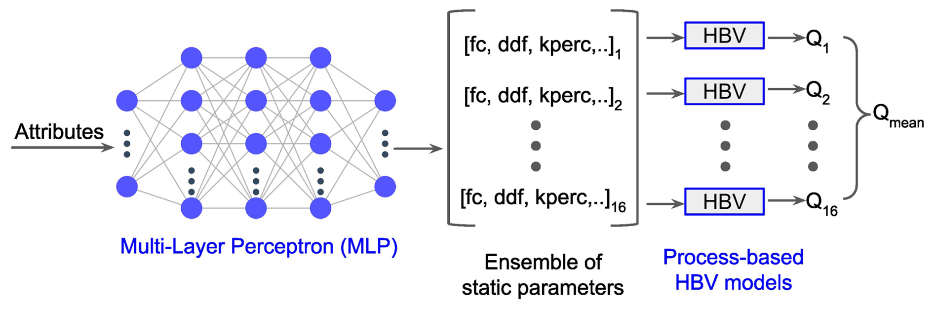
Figure 2 Schematic of differentiable MLP with ensemble HBV architecture with 16 independent modules.

2.3.2 LSTM + HBV and LSTM + 16HBV

The second network architecture uses an LSTM to estimate HBV parameters. In the LSTM + HBV architecture (Fig. 1b-c), the LSTM takes as input the same 30 static features used in the MLP, along with 3 dynamic features – precipitation, temperature, and daylength (see Table 1). Static features are repeated at every timestep within the LSTM lookback period, which is fixed at 365 d in this study. The LSTM is developed in a sequence-to-one configuration and uses linear activations in the output layer. Again, the resulting outputs are normalized between [0,1] using sigmoid activation and scaled to parameter-specific minimum and maximum ranges for the HBV model (Table B1).

During training (Fig. 1b), each instance consists of: (1) a 3-year sequence of precipitation and temperature forcings for the HBV model (ℝ^1095×2); and (2) a 1-year concatenated sequence of static and dynamic input features from the most recent year of the 3-year period (ℝ^365×33). This 1-year input sequence is passed through the LSTM, which transforms the inputs over the lookback period into a sequence of hidden states of equal length. In the sequence-to-one configuration adopted here, only the hidden state at the final timestep is extracted to produce static parameters for the HBV model (ℝ²⁰). As in the MLP + HBV model, these parameters, together with the 3-year forcing sequence, are then passed to the HBV model to simulate streamflow, and output from only the last of the three years is used to calculate the loss and update the LSTM weights.

During training of the LSTM + HBV model, HBV parameters are static for each input sequence, but they vary across different input sequences in the training period (denoted seq₁, …, seq_n in Fig. 1b). To obtain a static HBV parameter set during inference (i.e., the test set; Fig. 1c), the entire input sequence for a basin (denoted seq_full in Fig. 1c) is passed through the LSTM in a single forward pass, and only the final hidden state is used to estimate the HBV parameters. For example, with 15 years of data, the full 15-year concatenated input sequence (ℝ^5475×33) is processed by the LSTM, and the final hidden state (at the end of year 15) is mapped to a single parameter vector (ℝ²⁰), ensuring one static parameter set per basin. These parameters are then used with the full forcing series (ℝ^5475×2) in the HBV model to generate streamflow simulations for the entire period. This approach is taken to enforce a single, basin-specific static parameter set for the entire test period.

The training and testing approach described above is similar to what the literature calls “static” parameterization (Feng et al., 2022, 2023, 2024), even though sequence-to-one LSTMs produce parameters that vary across sequences during training. Another common approach – though not one taken here – is hybrid parameterization, where most parameters are treated as “static” (i.e., estimated based on the last time step of each sequence), while a subset is allowed to vary dynamically (i.e., estimated for all time steps in the LSTM's lookback period based on a sequence-to-sequence formulation) (Acuña Espinoza et al., 2025; Feng et al., 2022, 2023, 2024). However, even under this hybrid parameterization scheme, parameters labeled as “static” still vary across training sequences.

Analogous to the ensemble MLP configuration (Fig. 2), the LSTM + 16HBV architecture extends the LSTM + HBV model by producing an ensemble of 16 HBV parameter sets (ℝ³²⁰). Each parameter set is passed to an independent HBV model, and the resulting ensemble of streamflow simulations is averaged to produce the final prediction.

2.3.3 Model training and hyperparameter tuning

For all model configurations, loss is calculated between predicted and observed streamflow (in mm d⁻¹) using mean square error (MSE), and neural network weights are updated via backpropagation using the ADAM optimizer (Kingma and Ba, 2017). We initialize training with a learning rate of 0.001, reduced by 90 % if validation loss does not improve for 5 consecutive epochs. Training is continued until validation loss shows no improvement for 10 consecutive epochs. A dropout rate of 40 % is applied to MLP hidden layers and to the final linear layer of the LSTM. Models are trained with a batch size of 128 sequences, and input sequences are created with a stride length of 60 d. For example, if one sequence consists of a 3-year time series input, the subsequent sequence is generated by shifting the start of the previous sequence forward by 60 d. This approach results in overlapping data sequences and showed a modest improvement in validation set performance.

Our choices for hyperparameters are similar to previous studies (Feng et al., 2022; Acuña Espinoza et al., 2024), with additional control over the total number of epochs and learning rate through early stopping based on validation performance. We performed grid search to optimize neural network sizes for each configuration, selecting the architecture that achieves the lowest validation set error. Details of the hyperparameter grid search are provided in Table C1, Appendix C.

2.4 Impacts of comprehensive versus alternative static input features

In differentiable models, the static inputs to the neural networks often consist of the same diverse set of catchment attributes – encompassing climate, topography, geology, land cover, and soil type – commonly used by pure LSTM models. The implicit assumption is that these basin attributes provide informative context for neural network-based parameter learning. To test this assumption, we evaluate the role of static features through two experiments that use alternative static feature sets relative to the reference case where models use the full set.

In the first experiment, the neural network receives only basin latitude and longitude as static input. This represents a scenario where models are deprived of all physical basin attributes and provided only with direct positional information.

In the second experiment, we use the same full static feature set as in the reference case, but we randomly shuffle the attribute vectors across all basins without replacement. This experiment represents a scenario where the neural network still receives comprehensive attribute features, but the values carry no physical information.

We then compare differentiable model simulations for out-of-sample evaluations in both time and space using these alternative static feature sets against the reference case trained with the full feature set. Note that while the MLP architecture uses only static features, the LSTM architecture also incorporates three dynamic features (precipitation, temperature, and daylength), which are held constant across all experiments.

2.5 Assessing temporal variability in LSTM-estimated parameters and the role of dynamic features

As discussed previously, the MLP architecture relies exclusively on static inputs and therefore produces a single, time-invariant set of parameters for each basin, analogous to conventional process-based models. In contrast, the sequence-to-one LSTM architecture generates sequence-dependent parameter sets during training and produces a single static parameter only during inference. This distinction motivates a closer examination of the extent to which the LSTM-based architecture introduces meaningful temporal variability into process-model parameters, and whether such variability is beneficial for streamflow prediction.

To quantify this behavior, we compute the coefficient of variation (standard deviation divided by mean) for each HBV parameter across training input sequences for each study basin. Two temperature-related parameters are excluded from this analysis because their mean values are close to zero, which would artificially inflate their coefficients of variation. For each basin, we then calculate the mean coefficient of variation across the remaining HBV parameters, yielding a single summary metric that characterizes the overall degree of temporal variability in LSTM-estimated parameters. We select representative basins exhibiting high, medium, and low variability and examine the temporal variation of individual HBV parameters in detail.

To understand how dynamic inputs contribute to HBV parameter learning for these basins, we apply an explainable AI technique known as Integrated Gradients (IG) (Sundararajan et al., 2017) to the LSTM-based differentiable model. More details are provided in Appendix D.

3 Results

3.1 Differentiable model performance in out-of-sample in time and space evaluation

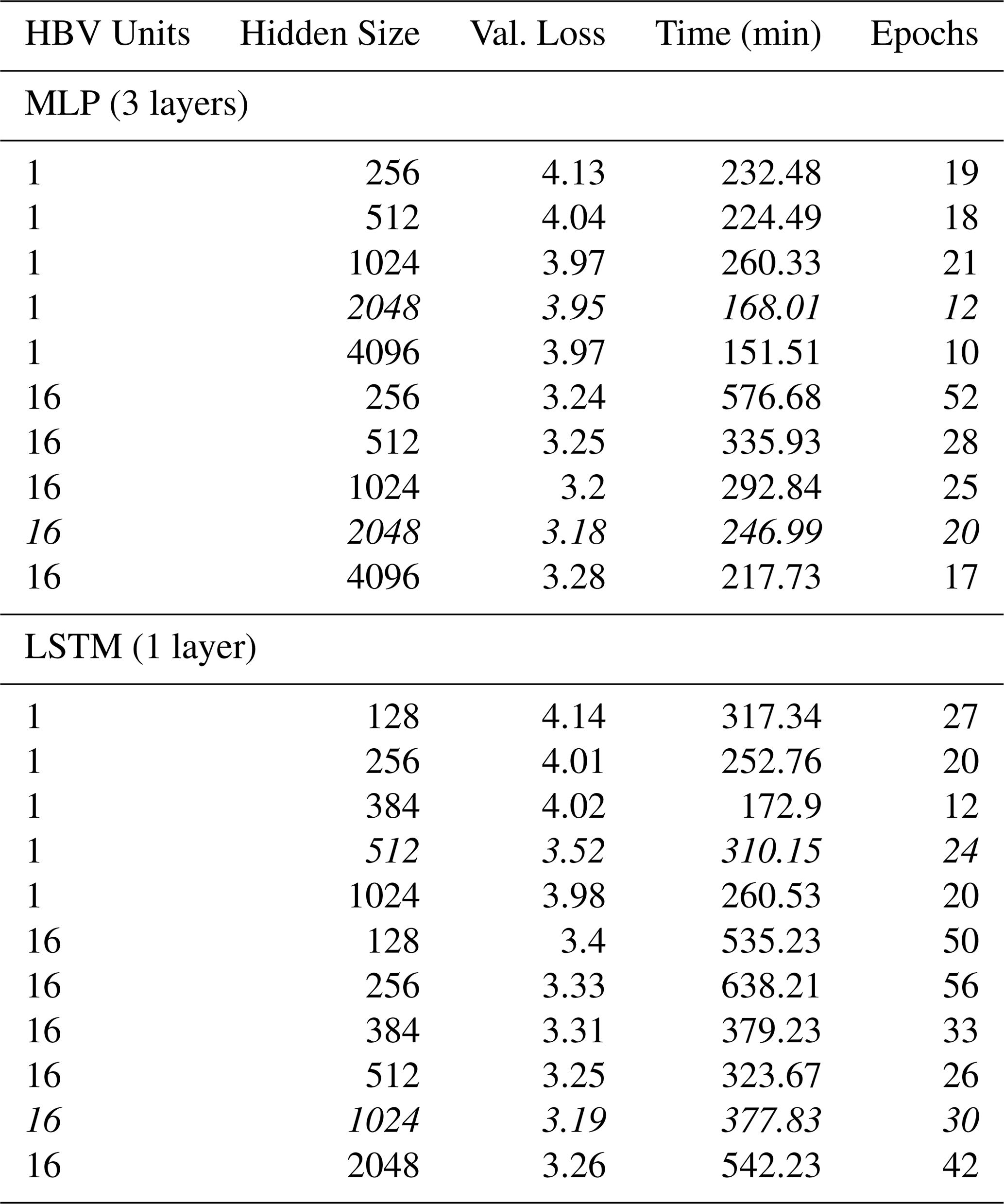
Hyperparameter tuning, detailed in Appendix C (Table C1), resulted in the following optimal neural network sizes:

1. MLP + HBV: 3 layers, each with 2048 nodes

2. MLP + 16HBV: 3 layers, each with 2048 nodes

3. LSTM + HBV: 1 layer with 512 nodes

4. LSTM + 16HBV: 1 layer with 1024 nodes

We used these optimized architectures for all four differentiable models and evaluated their temporal and spatial out-of-sample performance.

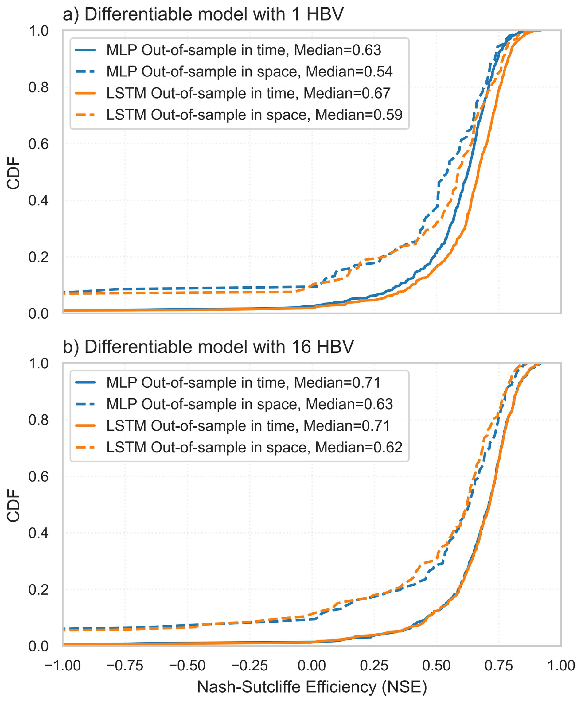
Figure 3 Cumulative distributions of Nash-Sutcliffe Efficiency (NSE) for out-of-sample in time and out-of-sample in space evaluations of MLP and LSTM-based differentiable model architecture using: (a) single-member HBV and (b) ensemble (16-member) HBV.

Figure 3 shows the distribution of Nash-Sutcliffe Efficiency (NSE) across in-sample gauges (solid lines) and out-of-sample gauges (dashed lines) for both single-unit (Fig. 3a) and ensemble-unit (Fig. 3b) model versions coupled with MLP (blue) and LSTM (orange) architectures. Several key findings emerge from this figure.

For single-unit HBV configurations (Fig. 3a), the LSTM-based architecture outperforms the MLP-based architecture in both out-of-sample in time and out-of-sample in space evaluations. Median NSE values increase from 0.63 to 0.67 for out-of-sample in time testing and from 0.54 to 0.59 for out-of-sample in space testing when using the LSTM instead of the MLP.

Introducing ensemble configurations (Fig. 3b) leads to substantial performance gains relative to single-unit models (Fig. 3a) for both neural network architectures and both evaluation settings, consistent with past work (Feng et al., 2022; Kratzert et al., 2018). However, under the ensemble configuration, the performance advantage of the LSTM over the MLP disappears. The cumulative NSE distributions for the two architectures are nearly indistinguishable, with identical median NSE values of 0.71 for out-of-sample in time evaluation and median values of 0.62 and 0.63 for LSTM- and MLP-based models, respectively, in out-of-sample in space evaluation. The reason why the LSTM outperforms the MLP under the single-unit configuration is not clear, but may reflect the additional flexibility provided by processing dynamic inputs when only one HBV parameter set is estimated. In the ensemble configuration, this difference is no longer evident, suggesting that the diversity of MLP-produced parameter sets may provide enough flexibility to achieve comparable performance without the added complexity of the LSTM.

Finally, we note that both ensemble-based architectures achieve the same benchmark performance of the ensemble, differentiable model applied to CAMELS-US in Feng et al. (2022), which was reported as having a median NSE of 0.714 in out-of-sample in time testing. Although there are differences between that study and the present work, including the training and testing periods, number of basins, and choice of loss function, overall model performance appears relatively insensitive to these methodological choices. To provide a more direct comparison, we also trained an ensemble-based MLP differentiable model using the same training period (1990 to 2005) and testing period (1980 to 1989) as Feng et al. (2022) and again obtained very similar performance compared to that study (Supplementary Figure S1).

We also evaluated the ensemble-based differentiable models across additional performance metrics, including the Kling-Gupta Efficiency (KGE), root mean square error (RMSE), percent bias, and flow-regime specific biases for high flows (top 10 % of observed flows), medium flows (30th to 90th percentiles), and low flows (bottom 30 % of observed flows) (Fig. 4). Across all metrics and flow regimes, the LSTM- and MLP-based architectures performed similarly in both out-of-sample in time and space evaluation. Taken together, these results suggest that ensemble-based parameter estimation provides clear benefits for differentiable hydrological modeling, but the added complexity of LSTM-based networks offers limited advantage over the simpler MLP-based approach.

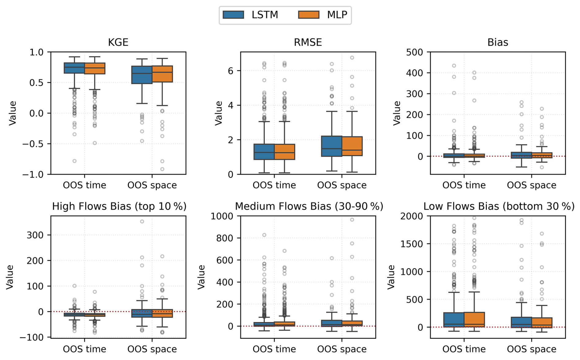
Figure 4 Performance of differentiable, ensemble-unit models with MLP- and LSTM-based architecture across multiple performance metrics for out-of-sample (OOS) in time and space evaluation.

3.2 Impacts of alternative static input features

Results in Figs. 3 and 4 are based on models trained with the full set of reference static input features. Figure 5 shows performance for ensemble-based models trained with two alternative static feature sets, the first of which only includes basin latitude and longitude and the second including the same comprehensive reference features but randomly mixed across basins. This experiment was performed only with ensemble-based models because of their demonstrated outperformance compared to single-unit models.

For the first experiment where only latitude and longitude were used as static input (Fig. 5a–b), we find similar NSE distributions compared to the reference input set for out-of-sample in space evaluations, both for MLP- (median NSE of 0.62 versus 0.63) and LSTM- (median NSE of 0.62 for both) based differentiable models. However, for out-of-sample in time evaluations, both differentiable models using only latitude and longitude showed substantial performance reductions, with a median NSE of 0.64 for the MLP-based model and 0.60 for LSTM-based model, as compared to a reference of 0.71 for both.

For the second experiment using full but nonsensical static inputs (Fig. 5c–d), we find little difference in the NSE distributions compared to the reference for out-of-sample in time evaluation, both for the MLP- (median NSE of 0.68 versus 0.71) and LSTM- (median NSE of 0.69 versus 0.71) based models. However, for out-of-sample in space evaluations, both differentiable models showed large degradation in performance, with a median NSE value of 0.47 against a reference of 0.63 for the MLP-based model, and a median value of 0.42 against a reference of 0.62 for the LSTM-based model.

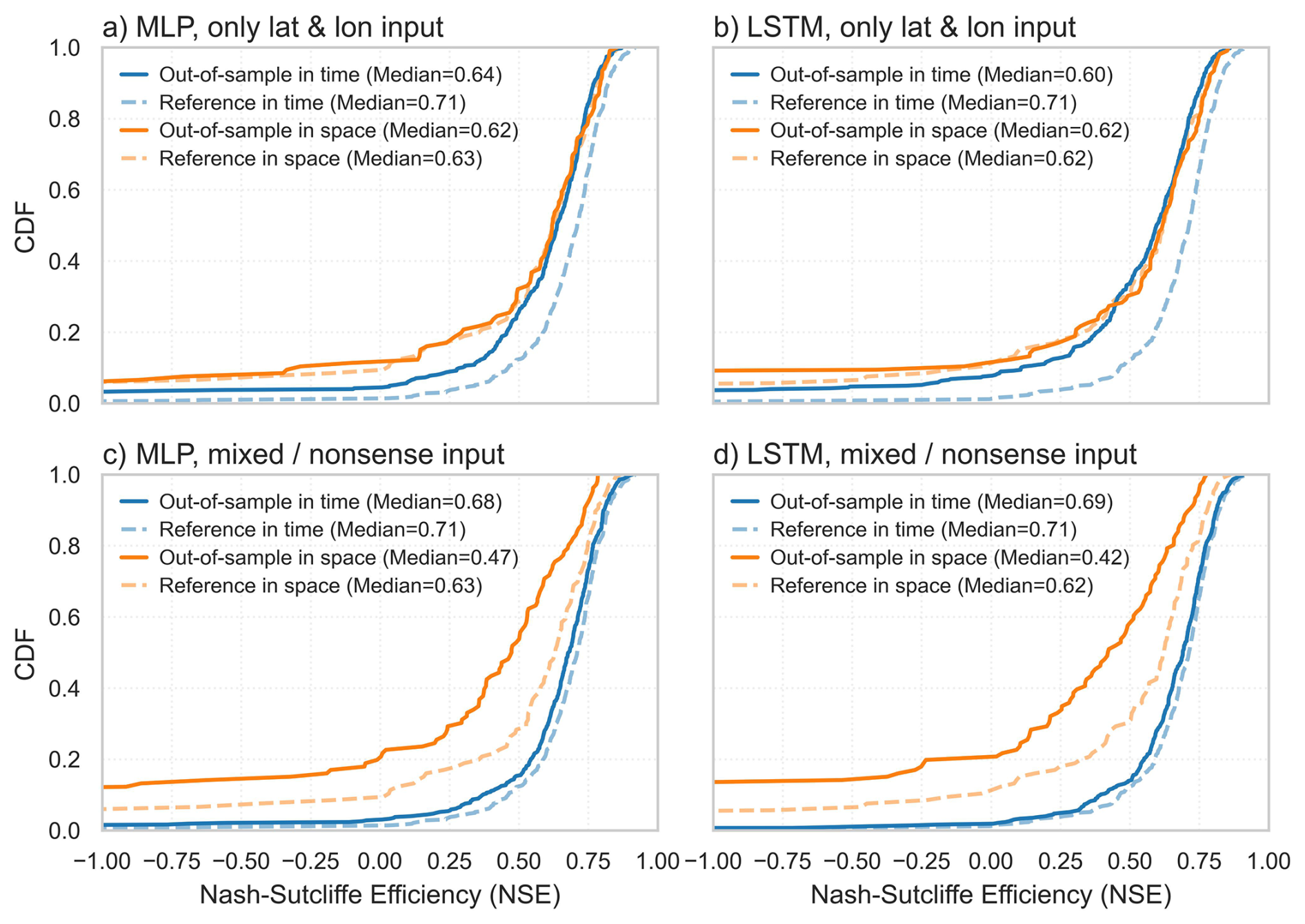
Figure 5 Cumulative distributions of NSE for out-of-sample in time and space evaluations of ensemble HBV differentiable models with (a) MLP using only latitude and longitude as static inputs, (b) LSTM using only latitude and longitude as static inputs, (c) MLP using comprehensive but randomly perturbed static features, and (d) LSTM using comprehensive but randomly perturbed static features. Dotted lines indicate reference performance using the comprehensive static feature set.

Table 2 Hypothesized roles of static input features in temporal and spatial generalization.

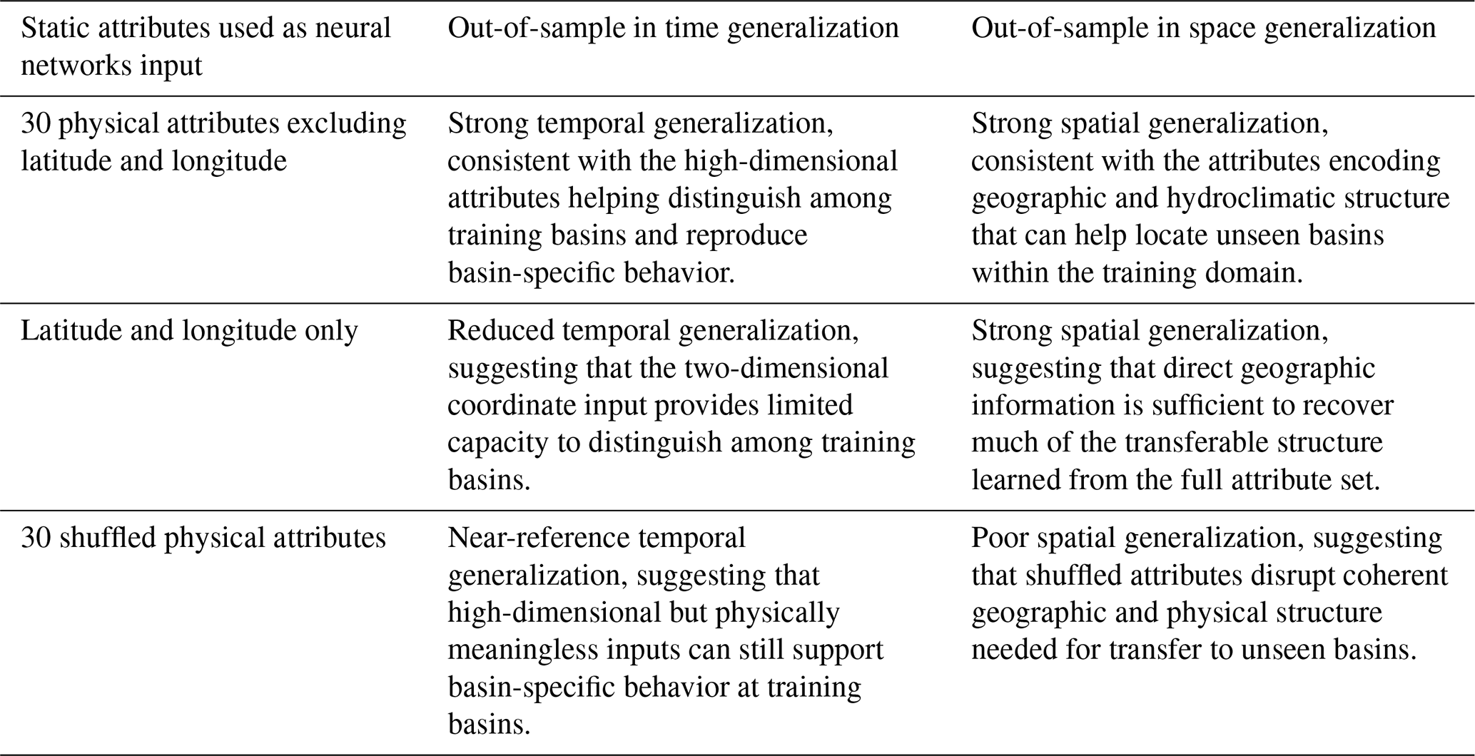
Overall, we find that the spatial generalization of differentiable models is largely preserved when latitude and longitude are used as the only static inputs. This result is plausible because many attributes in the full feature set, including climate, topography, geology, soils, and land cover, are spatially autocorrelated and therefore provide indirect information about where a basin is located. Thus, in these experiments, the comprehensive basin attributes may function largely as geospatial proxies rather than serving primarily as direct representations of physical controls on hydrological response (e.g., that high clay content leads to faster runoff). If the full attribute set were providing substantial additional transferable information about physical process controls, we would expect the reference model to show clearer improvements in spatial generalization relative to the latitude-longitude-only model. Instead, the two models perform similarly in out-of-sample basins. Temporal generalization, however, degrades when using only latitude and longitude, suggesting that the low-dimensional coordinate input provides less capacity for the model to distinguish among individual training basins and reproduce basin-specific behavior. This interpretation is further supported by the shuffled feature experiment, where providing comprehensive but nonsensical feature sets enables near-reference performance at the training basins but substantially reduces the ability to generalize spatially, because the shuffled features no longer preserve coherent geographic structure. Table 2 summarizes these experimental results and our hypotheses about how different static input features may support temporal and spatial generalization.

3.3 Assessing temporal variability in LSTM-estimated parameters and the role of dynamic features

Here we examine the nature of parameter estimates by the LSTM + HBV differentiable model, with particular emphasis on their temporal stability and the influence of dynamic inputs. To simplify interpretation, we focus on the single-unit LSTM + HBV configuration rather than the ensemble-based LSTM + 16HBV model.

Figure 6 summarizes the average coefficient of variation of HBV parameters across input sequences for each study basin. Most basins exhibit low variability, suggesting that the LSTM-based architecture does not utilize dynamic features to vary parameter estimates across sequences. There are some basins with a higher degree of parameter variability across training sequences, particularly in the central US. However, the average coefficient of variation across parameters never exceeds 0.2 for any site.

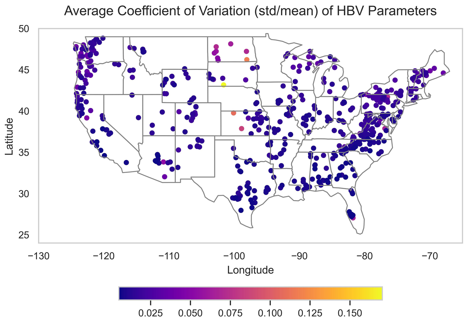
Figure 6 Spatial distribution of the average coefficient of variation of HBV parameters between input sequences estimated by the LSTM + HBV differentiable model. Each dot represents a study basin, with color intensity indicating the magnitude of the average temporal variability of the parameter set.

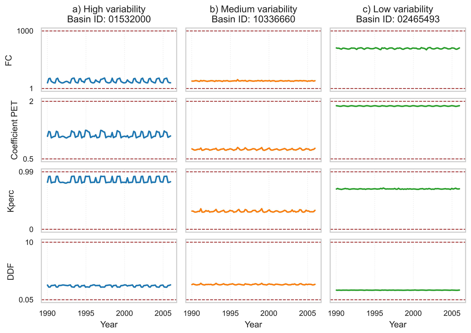
Figure 7 Temporal variability of four selected HBV parameters inferred by the LSTM + HBV differentiable model for basins exhibiting (a) high, (b) medium, and (c) low average coefficients of variation. The red dashed line shows the lower and upper bound for each parameter. Results are shown for the training period only, as LSTM-produced parameters vary during training whereas a single parameter set from the last time step is applied across the full period during testing.

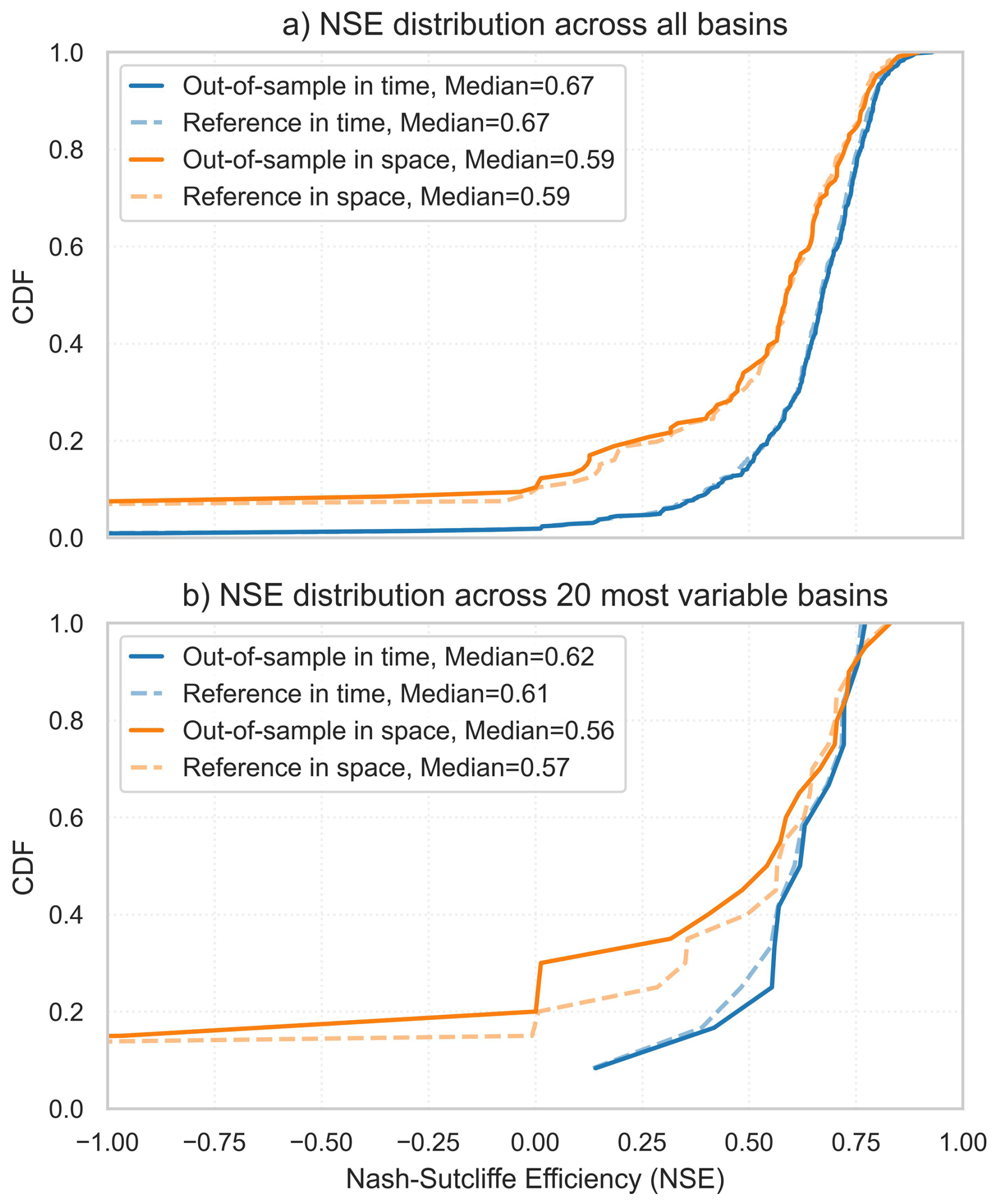
Figure 8 Cumulative distributions of NSE for out-of-sample in time and out-of-sample in space evaluations for the differentiable LSTM + HBV model using sequence-varying parameters for (a) all study basins, and (b) the 20 basins with highest parameter variability. Dotted lines indicate reference performance using a single static parameter from the final LSTM time step.

To further examine this behavior, we focus on three representative basins with high, medium, and low parameter variability (USGS IDs 01532000, 10336660, 02465493). Although the HBV model has 20 parameters, we present results for four illustrative parameters: field capacity (FC), coefficient of potential evapotranspiration (Coeff PET), coefficient of percolation (Kperc), and degree-day factor (DDF). Figure 7 shows the temporal variability of these parameters across input sequences for basins with (a) high, (b) medium, and (c) low variability.

In the low-variability basin, parameter estimates show negligible temporal variability across sequences, indicating that the LSTM effectively produces static parameters. In contrast, the medium- and high-variability basins exhibit progressively more parameter variability, although to varying degrees for different parameters. For example, in the high-variability basin, DDF exhibits comparatively limited temporal variation relative to the other three parameters. Additionally, several parameters tend to co-vary: FC, Coeff PET, and Kperc follow correlated seasonal cycles, reaching maxima and minima simultaneously, whereas DDF tends to vary out of phase, peaking when the other parameters are at their minima. Similar, though less pronounced, patterns are observed in the medium-variability basin. Feature importance based on Integrated Gradients shows that the differentiable model consistently relies more on static features than dynamic features (precipitation, temperature, and daylength) for HBV parameter estimation, even in the basin with high parameter variability (Fig. D1 in Appendix D), consistent with the limited variability in parameter values across sequences.

It is worthwhile to ask how the temporal variability in LSTM-based parameter estimates, where present, influences streamflow simulation. To investigate this, we compared two approaches to HBV simulation. In the first approach, model simulations were based on a single, static parameter set extracted from the final hidden state of the LSTM after processing the full input sequence for the test period. This is the reference case and is the same as shown in Fig. 1c. In the second approach, simulations are based on sequence-varying parameters, i.e., running the LSTM on rolling sequences during the test period. With a stride of 60 d, the input sequence shifts forward by 60 d at each step, generating new parameters every 60 d throughout the test period. This approach mirrors the training procedure as shown in Fig. 1b and represents a more natural inference method for sequence-to-one LSTMs. Thus, the first approach runs HBV with one parameter set for the entire test period (dashed lines in Fig. 8), while the second uses time-varying parameters that update every 60 d (solid lines in Fig. 8).

Figure 8a presents the distribution of NSE values across all basins for these two cases, while Fig. 8b focuses exclusively on the 20 basins exhibiting the highest degree of temporal parameter variability. In both cases, results show little difference in performance across basins. There are some small differences in the out-of-sample in space evaluation for basins with high temporal parameter variability (Fig. 8b), but it is the reference case (a single static parameter set) that outperforms the time-varying parameter models in this situation. These results are for a 60 d stride, selected because shorter strides did not improve validation performance. We also repeated this analysis with a 1 d stride, allowing parameters to vary at every time step, and found results consistent with the 60 d case (Supplement Figs. S2 and S3).

Together, these findings suggest that although the LSTM produces sequence-varying parameter estimates, exploiting this variability during inference does not yield meaningful performance improvements relative to using a single static parameter set derived at the end of the full forcing test sequence. Consequently, the observed temporal variability in LSTM-predicted parameters may reflect equifinality rather than dynamically evolving process parameters. If the time-varying parameters were capturing physically meaningful process variability, we would expect them to adapt to changing hydrologic conditions in ways that improve streamflow simulations relative to a single static parameter set from the final time step. We do not observe such improvements here. This conclusion applies to the sequence-to-one LSTM formulation used in the present study and may not extend to sequence-to-sequence formulations such as those in Feng et al. (2022) and Acuña Espinoza et al. (2024).

4 Discussion and Conclusion

Differentiable hybrid models that use machine learning to estimate parameters for process-based models show strong potential for achieving state-of-the-art performance while maintaining transparency of internal hydrological processes (Feng et al., 2022, 2023). Their rapid adoption reflects this promise. However, several aspects of differentiable model development have not received sufficient scrutiny, risking a shift toward prediction-driven modeling that undermines transparency and contradicts the philosophy of physics-based machine learning (Karpatne et al., 2017). This study addresses several such concerns by revisiting static and dynamic differentiable models and investigating key architectural decisions including neural network choices, process-based model configuration, and input requirements. We evaluate these models based on out-of-sample performance as well as interpretability. Our main conclusions and their implications for future differentiable model development are as follows:

1. In ensemble-based configurations, simpler MLP-based static parameterization matches the performance of dynamic LSTM-based parameterization.

   Differentiable models with ensemble configurations consistently outperformed single-unit models across both temporal and spatial test cases, consistent with previous findings (Feng et al., 2022, 2023). This result is expected and aligns with the multi-parameter ensemble literature that shows improved prediction accuracy by representing parametric uncertainty through ensemble aggregation (Beven and Binley, 1992; Blasone et al., 2008; Chiang et al., 2017; Shin et al., 2023).

   More importantly, in the ensemble-based configuration, simpler MLP-based differentiable models matched the performance of sequence-to-one LSTM-based models. MLP-based models achieved a median NSE of 0.71 in temporal testing for CAMELS-US basins, comparable to sequence-to-one LSTMs (0.714) and sequence-to-sequence LSTMs (0.732) reported by Feng et al. (2022). Similar results are found for spatial generalization. In addition, MLPs offer greater transparency by producing single, basin-specific process model parameters, which are not available in the same way from LSTM-based formulations. Because these basin-specific parameters, along with their corresponding internal state variables, can be examined using well-established diagnostic tools for process-based hydrologic models (Clark et al., 2017), MLP-based architectures provide a more accessible framework for assessing whether the model produces the right answer for the right reason (Kirchner, 2006). By contrast, the sequence-varying nature of LSTM-estimated parameters makes such diagnostics considerably more challenging. Together, these results provide a strong argument for considering more parsimonious, MLP-based architectures in future differentiable hydrological modeling.

   However, this interpretability advantage does not by itself imply that MLP-based models are more physically realistic or more fit for purpose. Rather, it means that they provide a more transparent and accessible framework for evaluating model behaviour through established diagnostic approaches. Moreover, the strongest performance of the MLP-based models occurs in the ensemble configuration, which itself can reduce interpretability. In this setup, the MLP predicts multiple static parameter sets, each of which is passed through a process-based model to generate an ensemble of streamflow predictions that are averaged before loss computation. This aggregation reduces transparency at the individual ensemble member level and raises questions about whether minimizing loss on the ensemble mean incentivizes physically consistent parameterization and internal state evolution within each member. It therefore remains unclear whether the improved streamflow simulations reflect greater physical fidelity or instead arise primarily from the statistical benefits of ensemble aggregation, analogous to how ensembles of weak learners can produce strong predictive models in methods such as random forests. Future work could address this issue by using loss functions that retain information about the full ensemble distribution rather than collapsing ensemble predictions to the ensemble mean, for example through scoring rule-based objectives (Vrugt, 2024). Thus, while MLP-based parameterization offers greater interpretability than LSTM-based approaches, these models still require rigorous internal diagnostics to determine whether their improved predictions are achieved for physically meaningful reasons. We identify this as an important future direction for improving process understanding in differentiable model development.

2. Differentiable models may use static basin attributes primarily as spatial proxies and for representing basin-specific behavior at training sites, rather than learning physical and transferable process controls.

   Recent work by Heudorfer et al. (2025) suggested that pure LSTM models may not be as entity aware as previously assumed, indicating that basin attributes provide limited information beyond meteorological forcings, especially for spatial generalization. We extend this insight to differentiable hydrological models through two experiments that examine how neural networks use static basin attributes.

   In the first experiment, we compared models using comprehensive basin attributes (climate, topography, geology, land cover, and soils) with models using only basin latitude and longitude as input. Spatial generalization did not degrade when only positional inputs were used, suggesting that comprehensive attributes may primarily encode basin location and serve as spatial proxies. This result is plausible in regional settings where similar basins are geographically clustered and where many catchment attributes are spatially autocorrelated. When models learn this spatial structure, they may generalize to unseen basins by placing them within an internally learned geographic representation. Consequently, for regions with dense and representative basin coverage such as CAMELS-US, latitude and longitude alone appear sufficient to recover much of the spatial generalization achieved using the full attribute set.

   However, this finding also raises an important limitation for extrapolation beyond the training domain. If the comprehensive basin attributes are used primarily to infer geographic location within the training region, rather than to learn transferable relationships between catchment properties and hydrologic response, then those same attributes may provide limited benefit when models are applied to hydroclimatically or physiographically distinct regions outside the training domain. For example, static attributes that help locate basins within CONUS may not support robust transfer to basins outside the United States unless the model has learned process-relevant mappings that remain valid across regions. Given the results presented here and in past work (Heudorfer et al., 2025), it remains unclear whether comprehensive static basin attributes support the kind of generalized mappings between catchment properties and hydrologic response needed for robust regional transfer. Additional research is needed to test this directly.

   In contrast, temporal generalization degraded when only latitude and longitude were used. We hypothesize that, in this case, using minimal (low-dimensional) inputs reduces the neural network's ability to differentiate individual basins. Because regional models are trained across basins simultaneously, distinguishing basins is necessary to learn basin-specific input-output relationships. To test this, we conducted a second experiment using the same comprehensive attribute vectors but with physically meaningless values, preserving input dimensionality without providing any physical information. Temporal generalization in this case matched performance obtained using physically meaningful attributes, supporting our hypothesis.

   Together, these results indicate that differentiable models may not be using static basin attributes primarily to learn physically meaningful relationships between catchment properties and hydrologic response. Instead, the attributes may function as spatial proxies that support generalization to nearby basins, while also providing high-dimensional identifiers that help reproduce basin-specific behavior at training sites. This finding underscores the need for methods that more directly leverage physiographic data to improve higher-order model generalization, particularly for extrapolating to conditions involving structural changes such as climate change and land-use modification (Heudorfer et al., 2025; Gupta, 2026). Our conclusions are based on ablation experiments rather than mechanistic interpretation of the networks themselves, which remains extremely challenging. It is still possible that neural networks extract some physically meaningful information from comprehensive basin attributes, and comparative performance under alternative input conditions does not prove that models treat those inputs equivalently. Nevertheless, the similarity between the full-attribute and latitude–longitude-only spatial generalization results suggests that physically meaningful attribute-response mappings may not be the dominant mechanism supporting spatial transfer in these experiments. Future studies should more directly investigate how neural networks map catchment properties to hydrological response.

3. LSTMs do not support true static parameterization. In sequence-to-one formulations, dynamic inputs contribute minimally, and time-varying parameters may reflect equifinality rather than seasonal dynamics.

   LSTMs operate in either sequence-to-sequence or sequence-to-one modes, generating parameters that vary at each timestep or across input sequences, respectively. In sequence-to-one implementations, the full input record for a basin can be used as a single sequence during testing, producing a single basin-specific parameter set. This is commonly labeled as a static parameterization in the literature (Feng et al., 2022, 2023), despite being trained with parameters that vary between input sequences. We evaluated how sequence-varying parameters influence streamflow simulations by comparing them with simulations generated using a single parameter set derived from the final timestep of the full input sequence. We did not find any meaningful differences between the two cases, suggesting that temporal variability in parameters with sequence-to-one implementation likely reflects cyclic manifestations of equifinality (Beven, 2006), rather than physically meaningful seasonal dynamics. This is further supported by the integrated gradients analysis, where dynamic inputs showed limited contribution in the parameter learning process. These findings contrast with a common assumption that time-varying parameters necessarily reflect changing physical system dynamics. While such relationships have been reported in sequence-to-sequence LSTM implementations (Feng et al., 2022), they do not appear to be the case for the sequence-to-one implementation presented in this work.

4. The conclusions of this study should be interpreted within the scope of the model formulations, attribution methods, and generalization experiments considered.

   There are several limitations of this work that warrant further discussion. First, this study focuses exclusively on sequence-to-one LSTM formulations, which have received less scrutiny than sequence-to-sequence approaches. Therefore, our conclusions may not generalize to sequence-to-sequence models, although others have already highlighted interpretability challenges with those formulations (Acuña Espinoza et al., 2024, 2025). Second, while integrated gradients provide useful insight into feature contributions, they do not capture interaction effects; future work should therefore consider alternative explainable AI approaches (e.g., Janizek et al., 2020) and ensure insights are robust across methods. Additionally, our generalization analysis is limited to out-of-sample temporal and spatial cases within a single region (CONUS). Evaluating transferability across regions and under climate non-stationarity remains an important next step.

   Finally, while MLP-based models yield interpretable, basin-specific parameters and match LSTM-based hybrid model performance, the MLPs themselves remain black-box function approximators. Replacing or augmenting MLPs with more interpretable architectures, such as Kolmogorov-Arnold Networks (KAN; Liu et al., 2025) that use learnable and visualizable activation functions, may enable deeper insight into internal model processes (Jing et al., 2025) and help identify mechanistic pathways between catchment properties and inferred process-model parameters. Our argument for more parsimonious MLP-based differentiable architectures therefore does not imply that they form an internally consistent model formulation. Rather, their static parameterization makes internal model diagnostics more tractable relative to LSTM-based dynamic parameterization. Important limitations also remain from the use of lumped process-model structures and the lack of explicit treatment of input and parametric uncertainties (Renard et al., 2010). Characterizing and representing these uncertainties is therefore another important area for future work in differentiable hydrological modeling. Together, these advances could support hybrid modeling frameworks that offer transparency not only in parameter estimation, but also in the representation of hydrological processes, which is critical for inference and decision-making under non-stationary conditions.

   In conclusion, this study highlights the value of parsimony in differentiable hydrological modeling. MLP-based differentiable models match the predictive performance of LSTM-based models while offering greater interpretability through static, basin-specific parameters. Comprehensive basin attributes appear largely redundant and potentially serve primarily as spatial proxies or mechanisms for representing basin-specific behavior at training sites, rather than enabling the learning of physically meaningful process controls. This suggests that increasing model complexity does not necessarily yield improved insights or generalization, and that caution is required when advancing differentiable hydrological models to promote improvements in both predictive skill and transparency.

Appendix A: Study area

The study area includes 531 basins (Fig. A1) from the CAMELS-US dataset. We used 80 % (n=425) basins for training and out-of-sample temporal testing, and 20 % (n=106) for out-of-sample spatial testing. The dataset includes basin physiographic attributes, meteorological forcings from multiple products (we used Daymet), and observed USGS streamflow data. Physiographic attributes are static, while meteorological and streamflow records are available at daily resolution from 1980 to 2014. Table 1 shows the attributes and meteorological forcings used in this study.

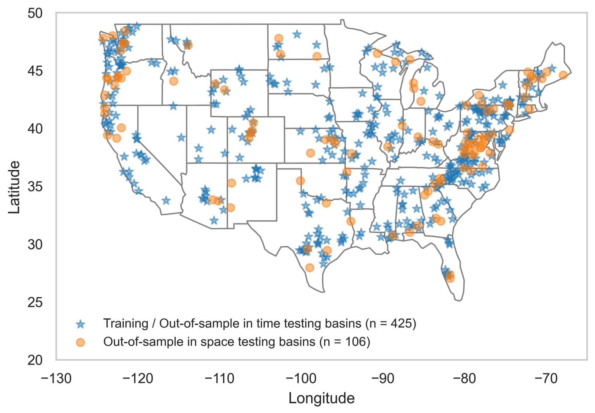
Figure A1 Study area showing the 531 CAMELS-US basins used in this study. Blue stars indicate basins used for training and out-of-sample in time testing (via temporal split). Orange dots indicate basins withheld entirely from training and used exclusively for out-of-sample in space testing.

Appendix B: Process-based HBV model

Our implementation of the process-based HBV model has 20 parameters across three interconnected modules; see Seibert (2005) for a detailed description of process representation. We follow the approach in Seibert (2005) with one key modification, where instead of single-parameter triangular routing, we use separate two-parameter gamma routing for direct flow and base flow. Table B1 shows the process representation, parameters, parameter descriptions, and bounds.

Table B1 HBV model parameters and feasible ranges.

Appendix C: Hyper-parameter tuning of differentiable models

For all four differentiable architectures, we tuned hyperparameters to determine the neural network size. The optimal architecture was selected using an early stopping criterion, defined as no decrease in validation loss for 10 consecutive training epochs. The hyperparameter tuning results are presented in Table C1, with the top-performing configuration italicized. Overall, the selected hyperparameter sets are justified not only based on validation performance but also in terms of reduced training time.

Table C1 Hyperparameter tuning results for four differentiable architectures, with the top-performing configuration italicized. All models use a stride length of 60 d.

Appendix D: Integrated Gradients analysis of LSTM-based differentiable model

This study employs an explainable AI technique known as Integrated Gradients (IG) (Sundararajan et al., 2017), which quantifies the contribution of each input feature to model predictions by integrating gradients along the path from a baseline input to the observed input. We applied IG to the LSTM-based, single-HBV unit differentiable model to assess how both static and dynamic inputs influence parameter estimation. For each daily HBV parameter prediction, the LSTM uses a one-year lookback period comprising concatenated static (30) and dynamic (3) input features (ℝ^365×33). We compute IG attributions for each of the 20 HBV parameters, yielding a three-dimensional attribution tensor over lookback period, input features, and HBV parameters (${\mathbb{R}}^{\mathrm{365}\times \mathrm{33}\times \mathrm{20}}$) for each prediction. This analysis is repeated for all timesteps in the testing period for each basin. Finally, we compute the average of the absolute IG values for each input feature and normalize the results such that the contributions across features sum to 100 %, providing an interpretable measure of the relative importance of static and dynamic inputs in HBV parameter learning. The results for basins with high, medium, and low parameter variability are shown in Fig. D1.

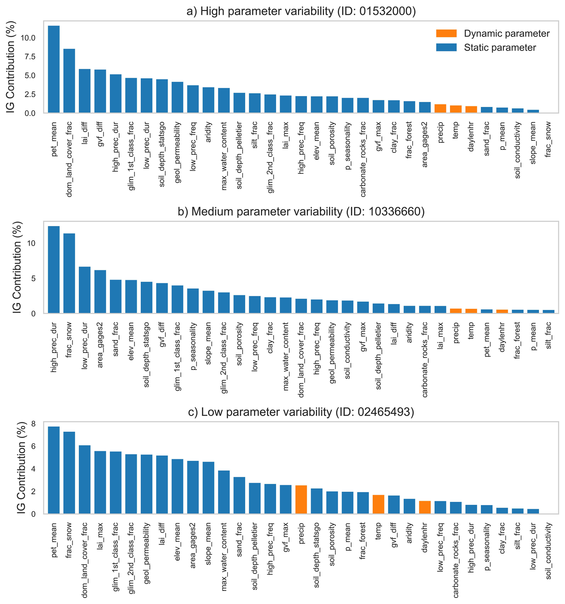
Figure D1 Feature importance for the LSTM + HBV differentiable hybrid model for basin with (a) high parameter variability, (b) medium parameter variability and (c) low parameter variability. Bars show the mean contribution of each input feature to parameter estimation, computed as the mean absolute integrated gradients and normalized to sum to 100 %.