BiasCast: learning and adjusting real time biases from meteorological forecasts to enhance runoff predictions

The use of deep learning models in hydrology is becoming an ever more prevalent application in operational flood forecasting. Such operational systems face performance degradation when transitioning from high quality reanalysis to meteorological forecast data with lower accuracy. This study investigates training strategies and Long Short-Term Memory network architectures to mitigate meteorological forecast-induced bias in maximum daily discharge predictions using the Extended LamaH- CE dataset and a subset of 451 basins. We systematically evaluated cross-domain generalization, transfer learning approaches, Encoder–Decoder LSTMs, Sequential Forecast LSTMs, and the role of input embeddings and integrating past discharge observations. The results show that domain shifts between reanalysis and forecast data lead to substantial skill loss, with median Nash–Sutcliffe Efficiency decreasing from 0.58 to 0.33. Among the tested strategies, the Sequential Forecast LSTM demonstrated the most stable improvements, achieving a median NSE of 0.63. Integrating recent discharge observations further enhanced performance, raising median NSE to 0.71 and surpassing even the reanalysis-driven baseline. In contrast, integrating archived forecasts or using more complex input embeddings did not yield consistent benefits and in some cases degraded model stability. Basin-level analysis reveals that forecast skill improvements compared to our baseline are not uniformly distributed across catchment types: the largest gains are concentrated in arid and precipitation-limited catchments, while alpine and snow-dominated catchments, despite experiencing the largest meteorological domain shift, show smaller improvements. This is likely because the LSTM cell state retains strong seasonal signals and thereby compensates for forecast input bias through its long-term memory mechanism, particularly in alpine and snow-dominated catchments where strong seasonal cycles dominate the hydrological response. These findings highlight the value of training strategies that allow models to directly learn bias correction during forecast transitions, emphasize the operational potential of combining sequential processing with near real-time discharge observations and identify physiographic catchment characteristics as key modulators of forecast skill improvement across diverse hydroclimatic settings.

1 Introduction

Accurate runoff prediction stands as one of the most critical challenges in modern hydrology, with far-reaching implications for flood risk management, water resource planning, and the design of resilient hydraulic infrastructure (Beven, 2012; Guo et al., 2021; Tran et al., 2025). While recent advances in deep learning have demonstrated that Long Short-Term Memory Networks (LSTMs) can effectively integrate multiple meteorological datasets to improve runoff simulation accuracy by learning complex spatial and temporal patterns (Kratzert et al., 2021), a fundamental challenge remains: operational forecasting systems rely on biased meteorological forecasts rather than reanalysis or observational data. This dependency introduces a cascade of uncertainties, as meteorological forecasts inherently exhibit lower accuracy and higher uncertainty than observational or reanalysis datasets (Lavers et al., 2021), with forecast errors further amplifying as lead time increases (Nester et al., 2012). The consequences of these uncertainties are particularly severe in flood forecasting applications, where timely and magnitudinally correct runoff predictions are critical for early warning systems and risk management (Chen et al., 2016).

The biases in meteorological forecasts stem from factors such as model resolution, data assimilation techniques, or orographic effects, and they differ depending on the numerical weather prediction model (e.g., ECMWF-HRES, DWD-ICON, NOAA-GFS), the predicted variable itself and the region in question (Haiden et al., 2024). These inaccuracies can propagate through hydrological models and lead to unreliable runoff forecasts, particularly under extreme conditions (Nester et al., 2012). To mitigate this issue, a variety of statistical and machine learning-based bias correction methods have been developed to adjust forecasted meteorological variables prior to their use as input in a hydrological model.

A simple approach to reduce biases in precipitation is described by Lenderink et al. (2007), who scale precipitation linearly based on a constant factor calculated from long term observations. To support operational warning systems, Hess (2020) developed the Ensemble Model Output Statistics (Ensemble-MOS) system, which postprocesses ensemble forecasts from COSMO-D2-EPS and ECMWF-ENS. The approach relies on logistic regression and stepwise multiple regression to reduce conditional biases and produce calibrated probabilistic forecasts efficiently. Ko et al. (2020) used the XGBoost machine learning algorithm to correct precipitation forecasts. Their method demonstrates that machine learning can improve rainfall forecasting performance, especially localized heavy rainfall events, which are of special importance for flash floods in small catchments. Zhang et al. (2020) used LSTMs to learn relationships between meteorological forecasts and observed rainfall data. Their results indicate that LSTMs are capable of learning dynamic biases to correct the forecasts from numerical weather predictions and increase forecast reliability, especially for heavy rainfall events. Han et al. (2021) proposed CU-net, a convolutional neural network architecture specifically designed to address systematic biases in gridded numerical weather predictions from ECMWF-IFS. Their grid-based approach represents a methodological advancement by directly correcting spatial forecast fields, enabling comprehensive bias mitigation across continuous meteorological domains. However, the focus on ECMWF-IFS data raises important questions about the correction model's transferability to other numerical weather prediction systems, potentially limiting the generalizability of their bias correction framework to broader operational contexts.

The studies mentioned have in common that the meteorological forecasts are compared either with meteorological station- or reanalysis data. In this context, it is important to note that especially precipitation measurements, whether from rain gauges, radar, or satellite sources, are inherently subject to various sources of uncertainty (Bárdossy et al., 2022). These errors stem from undercatch due to wind effects or sensor limitations (Yang et al., 1999). As a consequence, it can be assumed that even when inputting bias corrected precipitation forecast data to a hydrological model, a source of uncertainty with potential error propagation also arises here, which in turn creates a bias in runoff prediction. In contrast, discharge observations are typically regarded as more reliable compared to precipitation observations, as they represent an integrated hydrological response over the entire catchment and are measured continuously at fixed gauging stations (Herrnegger et al., 2015; Mao et al., 2019). Although discharge measurements also carry uncertainty, particularly related to the use of rating curves or sensor malfunction during extreme events, they are less affected by spatial representativeness errors, e.g. compared to precipitation, which requires spatial interpolation from a network of point measurements (De Oliveira and Vrugt, 2022; Villarini et al., 2008).

A method directly improving streamflow forecasts from the physically based Global Flood Awareness System (GloFAS) was developed by Hunt et al. (2022). GloFAS is an operational hydrological forecasting system that couples ECMWF ensemble weather predictions with the LISFLOOD hydrological model to provide streamflow forecasts for rivers worldwide (Alfieri et al., 2013). Instead of bias-correcting the meteorological input variables, Hunt et al. (2022) addressed systematic biases in streamflow forecasts using a statistical bias correction method based on quantile mapping (QM) with spatial optimisation and subsequently applied a damping factor to blend the corrected forecasts with the original raw output. Despite the demonstrated improvements in forecast skill, this bias correction approach has several limitations. First, while the quantile mapping correction is not strictly limited to GloFAS and could in principle be applied to other distributed hydrological forecasting systems, it requires a hydrological forecast at the specific location of interest, which may not be available for all catchments, particularly smaller or poorly monitored ones. Second, the method is lead-time independent, meaning it does not account for the evolution of forecast bias over longer lead times, which can reduce its effectiveness for medium- to long-range forecasts. Third, the applied damping factor, while effective in reducing over-correction, is empirically tuned, which may limit its robustness when applied across diverse catchments or under changing climate conditions. A further limitation of the study is the relatively small number of catchments used (10 gauges), which constrains the generalizability of the findings.

Building on the idea that runoff observations may be more accurate than those of meteorology, Kirchner (2009) proposed a paradigm shift through the concept of “doing hydrology backward”, where discharge is used as the primary constraint to infer the dynamics and uncertainties of upstream processes, such as precipitation or evapotranspiration. Rather than relying solely on uncertain meteorological inputs to predict runoff, backward hydrology extracts information about catchment dynamics directly from the discharge time series itself (Herrnegger et al., 2015; Kirchner, 2009). In this respect, the approach could also be used to perform a dynamic bias correction of multiple meteorological forecast variables since runoff data may serve as a more robust target variable in data-driven modelling frameworks than uncertain meteorological observations (e.g. rainfall). Given the hypothesis that large-scale hydrological datasets contain more information than could be described using theoretical or conceptual approaches (Nearing et al., 2021), a way to harness the potential of machine learning is to combine large sample datasets with meteorological forecasts as inputs. In such a setup, the model can learn to assign weights to the forecasts and internally correct their biases, thereby improving the overall runoff prediction accuracy.

In this study we investigate multiple Long Short-Term Memory (LSTM) network architectures and training strategies to reduce meteorological forecast-induced bias in 24 h ahead maximum daily discharge predictions. The focus on daily maxima ensures that critical peak flows relevant to flood forecasting are not masked by temporal averaging. 24 h lead time was selected as an initial proof-of-concept to establish baseline performance of bias correction capabilities, as forecast uncertainty generally increases with lead time (Nester et al., 2012), making shorter horizons an appropriate starting point for validating the approach while providing a foundation for future extension to multi-day predictions. We evaluate baseline LSTM configurations, transfer learning approaches, encoder–decoder architectures, and sequential LSTM networks across 451 catchments from the Extended LamaH-CE dataset in Central Europe. Our experiments examine the effectiveness of different data integration scenarios, including the incorporation of past discharge observations and archived forecasts, with the goal of developing robust neural network-based approaches for operational flood forecasting systems that can effectively compensate for systematic biases inherent in numerical weather prediction models.

2 Data and Methods

2.1 Data

This study uses an extended version of the daily LArge-SaMple DAta for Hydrology and Environmental Sciences for Central Europe (LamaH-CE; Klingler et al., 2021). LamaH consists of 859 gauged catchments including 21 catchment averaged meteorological variables, with more than 60 static catchment attributes. Since the original version of LamaH only contains meteorological ERA5-Land data and Kratzert et al. (2021) show that leveraging multiple meteorological data sources is beneficial in large sample hydrology, we expanded the data by 15 further variables from five sources. The products used are (i) ERA5-Land (Muñoz-Sabater et al., 2021) as in the original LamaH data, (ii) ECMWF-HRES European Center for Medium Range Weather Forecast - High Resoultion Forecast (ECMWF, 2025), (iii) E-OBS gridded observational data (Cornes et al., 2018), (iv) MSWEP multi-source weighted ensemble precipitation (Beck et al., 2019) and (v) GLEAM global land evaporation Amsterdam model (Miralles et al., 2011). Details of the variables used, including their definitions, units, and sources, are summarized in Appendix A. The data products were obtained as raster data and subsequently aggregated to the LamaH basins. All variables are daily averages (e.g. temperature) or daily sums (e.g. precipitation). For the ECMWF-HRES variables temperature, dew point and sea level pressure, 3 hourly forecast values (8 per day) were calculated as daily averages starting from 0 o'clock (UTC) issue time. A second adaption we made to the LamaH dataset concerns the gauge files. In the daily version of LamaH-CE, there are only the mean daily discharges – we have extracted the daily minima and maxima from the hourly LamaH data for all gauges and extended the daily version with those.

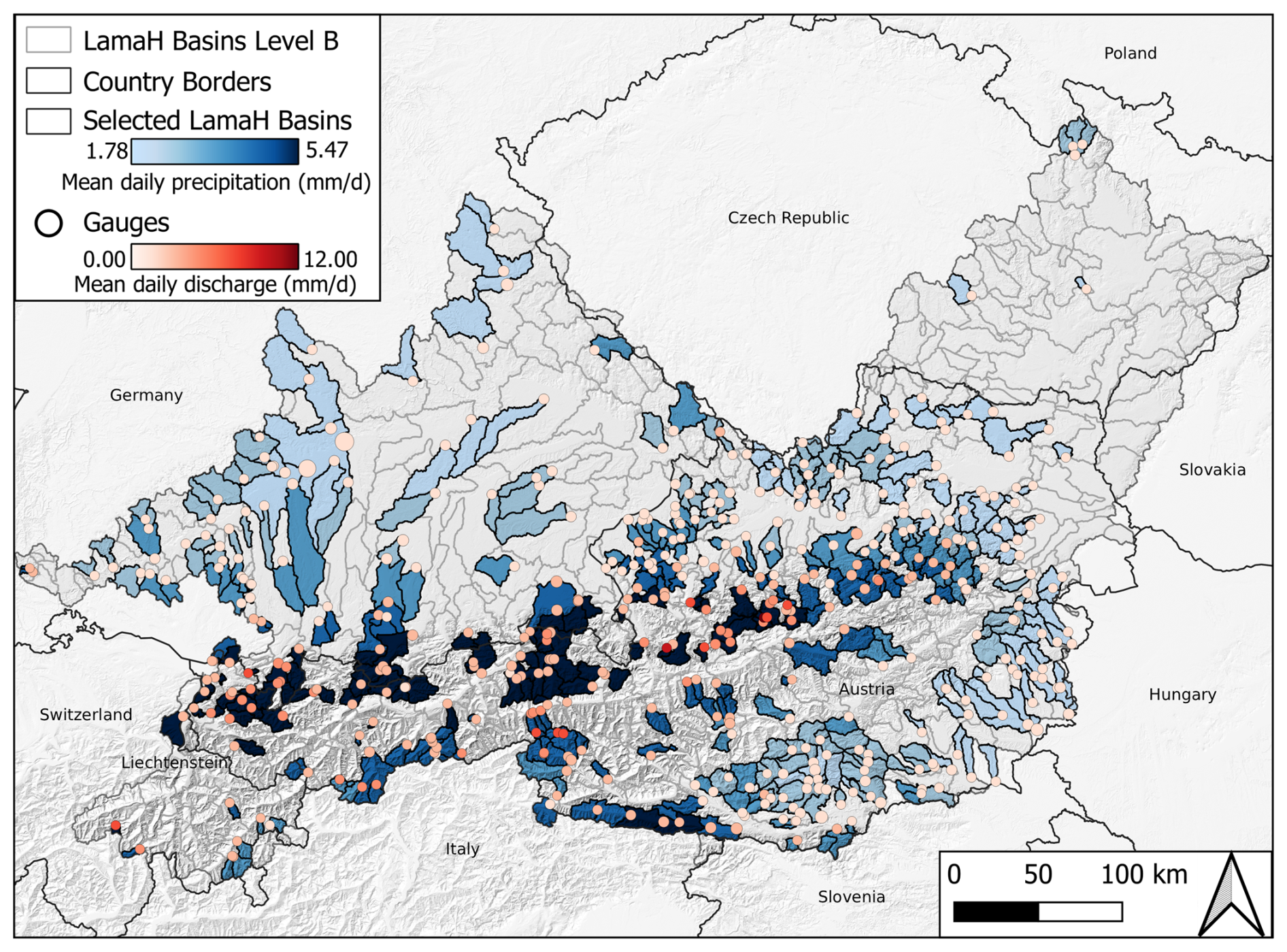
Figure 1 LamaH domain with the 451 subset basins. For better illustration, LamaH subbasins (level B, blue polygons) are shown here, but calculations were performed at LamaH level A (lumped for each gauge). The red points show the runoff gauges located at the catchment outlet.

For the conducted experiments, we used a subset of 451 basins with no and low anthropogenic influence at LamaH aggregation level A, which represents the lumped topographic catchment area of a gauge. Level A is comparable to the aggregation of the catchment areas in the CAMELS (Newman et al., 2015) dataset. The catchments are spatially distributed across the entire LamaH domain, with catchment areas including high alpine-, alpine foothill- and lowland areas. The subset includes both headwater and nested catchments, with 72.5 % of the basins being headwater catchments and 27.5 % being nested, meaning they have at least one other gauged basin from the selection upstream.

2.2 Experimental design

To comprehensively evaluate the performance of LSTM-based flood prediction models under different data availability scenarios and training strategies, we designed five distinct experimental groups with the primary research question: How to reduce the meteorological forecast induced bias in runoff predictions?

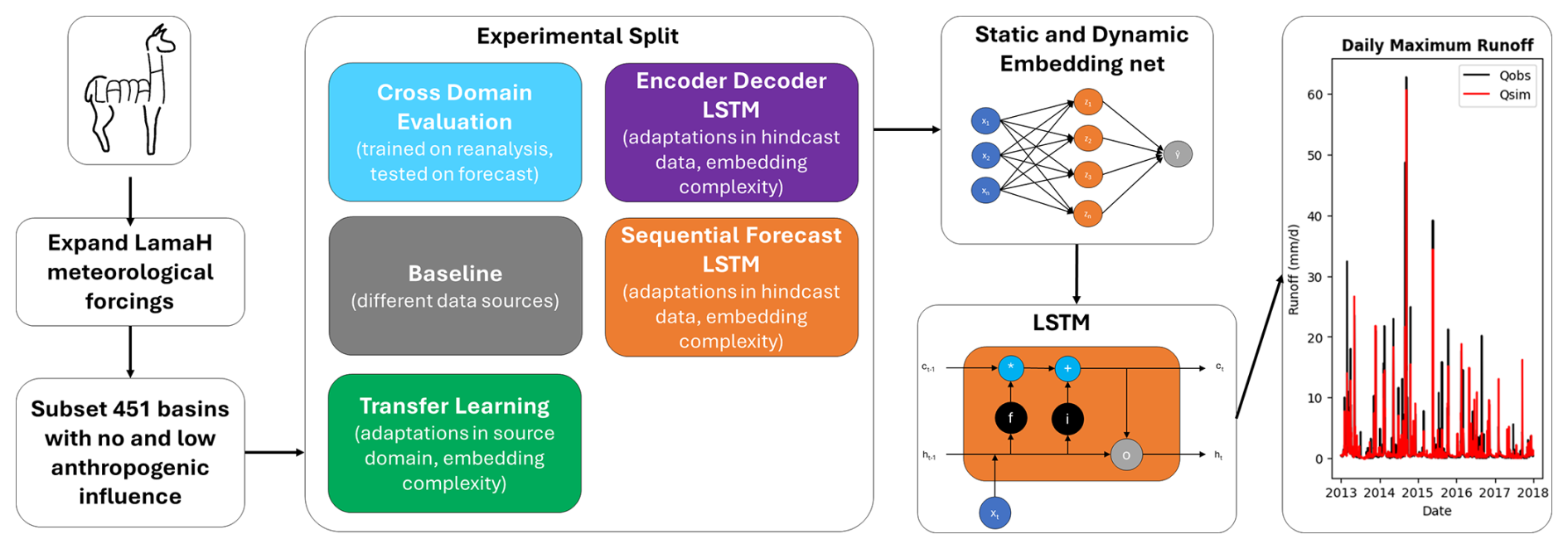
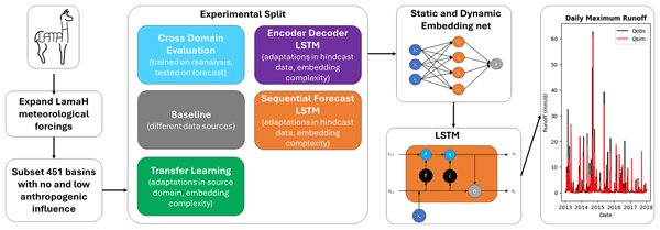
Figure 2 Workflow of the conducted experiments. The LamaH-CE dataset was extended by forecast and further reanalysis data and subset to 451 basins with no and low anthropogenic influence. The experimental split is divided into the deep learning architectures used, followed by a schematic representation of input embeddings for static and dynamic variables which feature space is fed to the LSTM. The last step is the forecast of the daily maximum runoff at the gauges.

All experiments were, in terms of reproducibility, conducted with the NeuralHydrology (Kratzert et al., 2022) python library and trained on different LSTM architectures to predict maximum daily discharge (q_max). The models incorporated dynamic meteorological inputs using a 365 d input sequence length, and static catchment attributes (33 physiographic, climatic, and land cover characteristics), both processed through separate embedding networks. The embedding networks are fully connected neural network layers that transform raw input variables into learned representations (Ahmed et al., 2023). A primary motivation for their use in this study is to enable transfer learning and consistent processing across experiments with different input dimensions. By projecting varying numbers of input variables from different data sources into a shared latent space, the model can be pre-trained on reanalysis and fine-tuned on forecast data regardless of differences in the feature space between domains. The experimental framework utilized a consistent temporal split with training data from 2003–2009, validation from 2010–2013, and testing from 2014–2017. Model performance was evaluated using basin averaged Nash-Sutcliffe Efficiency (NSE*, Kratzert et al., 2019c) as the primary loss function. A description of the loss function is attached in Appendix C. Model hyperparameters, such as the number of hidden units, were optimized using Bayesian optimization (see Snoek et al., 2012) with NSE* as the objective function. A detailed description of the performed hyperparameter tuning is attached in Appendix D. Hereafter, we use the term “domain” in its machine learning sense, referring to a specific data distribution characterized by its feature space and statistical properties, rather than in its common hydrological meaning of a geographical region. Throughout the remainder of this paper, domain specifications and equations reference only dynamic meteorological forcings for clarity, with the understanding that static catchment attributes remain unchanged across all experimental setups.

2.2.1 Baseline

Three baseline experiments were conducted to establish performance benchmarks using different meteorological data sources in a standard LSTM runoff simulation framework. LSTMs are a special form of recurrent neural networks, mainly used for sequential (time series) data (Hochreiter and Schmidhuber, 1997). For a detailed description of the LSTM in relation to hydrological modelling, we refer to Kratzert et al. (2018, 2019b, c). The core tensor equations of the LSTM model responsible for the information flow are presented in Appendix E.

The baseline experiments were conducted using either forecasting data only (FC), reanalysis data only (RA), or a combination of both (FCRA) as dynamic inputs. Following Seibert et al. (2018), who argue that model performance can only be meaningfully interpreted when evaluated relative to benchmarks representing what could and should be expected, the FC experiment, forced only with archived forecasting data from ECMWF HRES, serves as a lower benchmark. Here, the 1 d lead-time ECMWF-HRES forecast is used for the full 365 d input sequence. The RA experiment, exclusively driven by all available reanalysis and observational data sources (ERA5-Land, E-OBS, MSWEP, and GLEAM), as described in Appendix A, establishes an upper benchmark for model performance under ideal hindcast conditions (i.e. retrospective simulations using quality-controlled historical data). The FCRA experiment extended the RA experiment by additionally incorporating the five ECMWF-HRES forecast variables as dynamic inputs alongside all reanalysis and observational data sources, representing the optimal data availability scenario.

The domains in the experiments formulate as:

$$\begin{array}{}\text{(1)}& {\displaystyle }{\mathcal{D}}_{\mathrm{FC}}=\mathit{\{}\left(x_t^{\mathrm{FC}},q_{\max ,t}\right){\mathit{\}}}_{t=\mathrm{1}}^T\text{(2)}& {\displaystyle }{\mathcal{D}}_{\mathrm{RA}}=\mathit{\{}\left(x_t^{\mathrm{RA}},q_{\max ,t}\right){\mathit{\}}}_{t=\mathrm{1}}^T\text{(3)}& {\displaystyle }{\mathcal{D}}_{\mathrm{FCRA}}=\mathit{\{}\left(x_t^{\mathrm{FC}}\cup x_t^{\mathrm{RA}},q_{\max ,t}\right){\mathit{\}}}_{t=\mathrm{1}}^T\end{array}$$

𝒟: Dataset used in the experiment; x_t: Meteorological variables at timestep t; q_max,t: Maximum daily discharge (target variable) at timestep t.

2.2.2 Cross-Domain Evaluation

The cross domain evaluation (CD) experiment examined model generalization by training on reanalysis data and testing on ECMWF-HRES forecast data while maintaining 5 identical input variables. The meteorological variables used in this experiment are temperature, dewpoint temperature, precipitation, solar radiation and actual evapotranspiration. This experimental design mirrors the operational framework of classic conceptual hydrological models, where models are typically calibrated using high-quality reanalysis data with subsequently applied real-time forecast inputs during operational usage. By replicating this established modelling paradigm within the LSTM framework, the experiment quantifies the performance shift when transitioning from reanalysis to operationally available forecast data. It is important to note that the CrossDomain experiment deliberately uses only five reanalysis variables, those with a direct equivalent in the ECMWF-HRES forecast data, in contrast to the Baseline Reanalysis which uses all 31 available reanalysis variables. The performance gap between these two configurations in Fig. 3 therefore reflects the additional benefit of combining multiple meteorological data sources, consistent with Kratzert et al. (2021). Our hypothesis here was that if the distributions of the two input data sets 𝒟_FC and 𝒟_{RA,CrossDomain} are too different, the model performance will decline.

The variables compared in the Cross Domain Evaluation can be taken from Table 1, with its domains in the experiments formulated as:

$$\begin{array}{}\text{(4)}& {\displaystyle }\text{Train on: }{\mathcal{D}}_{\mathrm{RA},\mathrm{CrossDomain}}=\mathit{\{}\left(x_t^{\mathrm{RA}},q_{\max ,t}\right){\mathit{\}}}_{t=\mathrm{1}}^T\text{(5)}& {\displaystyle }\text{Test on: }{\mathcal{D}}_{\mathrm{FC}}=\mathit{\{}\left(x_t^{\mathrm{FC}},q_{\max ,t}\right){\mathit{\}}}_{t=\mathrm{1}}^T\end{array}$$

Table 1 The five meteorological forcing variables shared between reanalysis and forecast, used in the Cross Domain Evaluation experiment to ensure an identical input feature space between training and inference. Variables were deliberately sourced from multiple dedicated products to combine the strengths of different data sources, reduce cross-correlation between input features, and avoid propagating systematic biases from a single reanalysis across all variables. Especially for total precipitation, MSWEP has shown to consistently outperform other precipitation datasets across diverse hydroclimatic settings (Abbas et al., 2026; Beck et al., 2017). A detailed description of all variables is provided in Appendix A.

2.2.3 Encoder–Decoder LSTM

The Encoder–Decoder LSTM developed by Nearing et al. (2024) consists of two connected LSTMs: one for the hindcast phase forced with historical meteorological reanalysis data (e.g. ERA5) and one for the forecast phase forced with weather forecast data. The two LSTMs are connected by a non-linear handoff network in which the cell state and hidden state from the hindcast are transferred to the forecast LSTM. This architectural design allows the forecast LSTM to learn hydrological states from the hindcast, which could be understood as initial conditions in the model.

Three distinct experiments were implemented using the Encoder–Decoder LSTM architecture to investigate if this dual-LSTM framework can learn and compensate dynamical biases inherent in meteorological forecasts. The first experiment with domain ${\mathcal{D}}_{\mathrm{ED}-\mathrm{LSTM},\mathrm{1}}$ implemented the basic encoder–decoder framework where the hindcast LSTM was forced with historical reanalysis data while the forecast LSTM processed meteorological forecast data. The second experiment with domain ${\mathcal{D}}_{\mathrm{ED}-\mathrm{LSTM},\mathrm{2}}$ extended this architecture by incorporating past mean daily discharge observations alongside reanalysis data in the hindcast LSTM. The third experiment with domain ${\mathcal{D}}_{\mathrm{ED}-\mathrm{LSTM},\mathrm{3}}$ extended ${\mathcal{D}}_{\mathrm{ED}-\mathrm{LSTM},\mathrm{2}}$ by additionally forcing the hindcast cell of the model with forecast data. This emulates a setting in which archived forecasting data are used in combination with reanalysis data in the hindcast phase.

The domains in the experiments formulate as:

$$\begin{array}{}\text{(6)}& {\displaystyle }{\mathcal{D}}_{\mathrm{ED}-\mathrm{LSTM},\mathrm{1}}={\left\{\left(x_{t-s:t-\mathrm{1}}^{\mathrm{RA}}\cup x_t^{\mathrm{FC}},q_{\max ,t}\right)\right\}}_{t=s+\mathrm{1}}^T\text{(7)}& {\displaystyle }\begin{array}{rl}& {\mathcal{D}}_{\mathrm{ED}-\mathrm{LSTM},\mathrm{2}}\\ & ={\left\{\left(x_{t-s:t-\mathrm{1}}^{\mathrm{RA}}\cup q_{\max ,t-s:t-\mathrm{1}}\cup x_t^{\mathrm{FC}},q_{\max ,t}\right)\right\}}_{t=s+\mathrm{1}}^T\end{array}\text{(8)}& {\displaystyle }\begin{array}{rl}& {\mathcal{D}}_{\mathrm{ED}-\mathrm{LSTM},\mathrm{3}}\\ & ={\left\{\left(x_{t-s:t-\mathrm{1}}^{\mathrm{RA}}\cup x_{t-s:t-\mathrm{1}}^{\mathrm{FC}}\cup q_{\max ,t-s:t-\mathrm{1}}\cup x_t^{\mathrm{FC}},q_{\max ,t}\right)\right\}}_{t=s+\mathrm{1}}^T\end{array}\end{array}$$

s: Sequence length.

2.2.4 Sequential Forecast LSTM

The Sequential Forecast LSTM experiment employs a two-phase sequential processing strategy to leverage both reanalysis and operationally available forecast data within a unified framework. The architecture consists of separate embedding networks for hindcast and forecast inputs, a shared LSTM layer and a state transfer mechanism that enables knowledge transfer between processing phases (see Sequential Forecast LSTM in NeuralHydrology, Kratzert et al., 2022). In the first phase, the LSTM processes embedded historical reanalysis data to generate hidden and cell states. The second phase continues LSTM processing with embedded forecast data, initialized with the states from the hindcast phase, ensuring that forecast predictions are informed by contextual information learned from historical patterns. The model generates predictions by concatenating outputs from both phases through a prediction head, with the optimization objective to maximize NSE*. This design enables optimal utilization of reanalysis data for learning hydrological patterns while maintaining operational forecasting capabilities through the state transfer mechanism.

Experiment one (𝒟_SEQLSTM,1) used the basic Sequential LSTM framework, with only using reanalysis data in the hindcast phase and forecast data in the forecast phase. The second experiment (𝒟_SEQLSTM,2) added to the first domain mean daily discharge observations alongside reanalysis data in the hindcast phase. In the third experiment (𝒟_SEQLSTM,3), we extended 𝒟_SEQLSTM,2 by additionally forcing the hindcast phase of the model with archived forecast data.

The domains in the experiments formulate as:

$$\begin{array}{}\text{(9)}& {\displaystyle }{\mathcal{D}}_{\mathrm{SEQLSTM},\mathrm{1}}={\left\{\left(x_{t-s:t-\mathrm{1}}^{\mathrm{RA}}\cup x_t^{\mathrm{FC}},q_{\max ,t}\right)\right\}}_{t=s+\mathrm{1}}^T\text{(10)}& {\displaystyle }\begin{array}{rl}& {\mathcal{D}}_{\mathrm{SEQLSTM},\mathrm{2}}\\ & ={\left\{\left(x_{t-s:t-\mathrm{1}}^{\mathrm{RA}}\cup q_{\max ,t-s:t-\mathrm{1}}\cup x_t^{\mathrm{FC}},q_{\max ,t}\right)\right\}}_{t=s+\mathrm{1}}^T\end{array}\text{(11)}& {\displaystyle }\begin{array}{rl}& {\mathcal{D}}_{\mathrm{SEQLSTM},\mathrm{3}}\\ & ={\left\{\left(x_{t-s:t-\mathrm{1}}^{\mathrm{RA}}\cup x_{t-s:t-\mathrm{1}}^{FC}\cup q_{\max ,t-s:t-\mathrm{1}}\cup x_t^{\mathrm{FC}},q_{\max ,t}\right)\right\}}_{t=s+\mathrm{1}}^T\end{array}\end{array}$$

2.2.5 Transfer Learning

Transfer Learning (TL) is a machine learning paradigm leveraging gained knowledge from a source domain to improve learning performance in a target domain (Goodfellow et al., 2016). Formally, TL aims to improve the predictive performance on the target domain using knowledge from the source domain, with differences potentially existing in the feature space, data distribution, or learning task between the two domains (Zhuang et al., 2021). TL can be categorized into two primary types based on the relationship between source and target domain: The first is homogeneous transfer learning, where both domains share the same feature space (i.e. using identical meteorological variables and catchment attributes) and have the same marginal probability distributions (Weiss et al., 2016). The second is heterogeneous transfer learning, where the feature spaces differ between domains (Pan and Yang, 2010). For our experiments, we used the heterogeneous transfer learning approach – while the learning task stays the same in the conducted experiments, namely predicting maximum daily discharges at a gauge, the feature spaces and its distributions between forecast (target domain) and reanalysis (source domain) data differs, as evidenced by the violin plots in Appendix B.

In the context of forecast bias reduction, transfer learning is used to leverage knowledge from the less bias-influenced reanalysis source data to improve prediction accuracy when applied to the more bias-prone forecast target data. This approach is particularly relevant in contexts involving hydrometeorological data, where reanalysis data represents a post-processed quality-controlled dataset with reduced systematic errors, while forecast data contains dynamical biases from numerical weather prediction models. By pre-training the temporal encoder (LSTM) on reanalysis data, the model learns hydrological process representations that can subsequently be fine-tuned to accommodate the bias characteristics of forecast inputs, potentially improving the model's ability to correct for systematic forecast errors while maintaining learned temporal dependencies.

The first experiment implemented full weight transfer learning, where all network weights from the baseline 𝒟_RA experiment (embedding networks, LSTM and output layers pre-trained on reanalysis data) were used as initialization for a new training phase on forecast data, allowing all parameters to be updated through backpropagation to adapt to the 𝒟_FC target domain's characteristics. The second experiment, also based on the weights of 𝒟_RA employed selective weight transfer learning, adapting only the dynamic embedding network weights while freezing other model parameters including the static embedding network, thus preserving learned temporal patterns while allowing adaptation to new forcing input characteristics. The third experiment applied the same selective transfer learning method as the second experiment, but network weights are based on the 𝒟_FCRA domain.

The domains in the experiments are given below with source and target domains as well as training objective. All three experiments are based on training either LSTM weights θ, embedding layer weights ϕ, output layer weights ψ or all combined with a NSE* loss function L_NSE().

$$\begin{array}{}\text{(12)}& {\displaystyle }\begin{array}{rl}{\text{TL}}_{\mathrm{AllWeights}}:& \text{ source domain }{\mathcal{D}}_{\mathrm{RA}},\text{ target domain }{\mathcal{D}}_{\mathrm{FC}}\\ & \text{ with objective }\arg \underset{\mathit{\theta },\mathit{\varphi },\mathit{\psi }}{\min }{L}_{\mathrm{NSE}}\left({\mathcal{D}}_{\mathrm{FC}}\right)\end{array}\text{(13)}& {\displaystyle }\begin{array}{rl}{\text{TL}}_{\mathrm{EmbeddingNet}\mathrm{\_}\mathrm{1}}:& \text{ source domain }{\mathcal{D}}_{\mathrm{RA}},\text{ target domain }\\ & {\mathcal{D}}_{\mathrm{FC}}\text{ with objective }\arg \underset{\mathit{\varphi }}{\min }{L}_{\mathrm{NSE}}\left({\mathcal{D}}_{\mathrm{FC}}\right)\end{array}\text{(14)}& {\displaystyle }\begin{array}{rl}{\text{TL}}_{\mathrm{EmbeddingNet}\mathrm{\_}\mathrm{2}}:& \text{ source domain }{\mathcal{D}}_{\mathrm{FCRA}},\text{ target domain }\\ & {\mathcal{D}}_{\mathrm{FC}}\text{ with objective }\arg \underset{\mathit{\varphi }}{\min }{L}_{\mathrm{NSE}}\left({\mathcal{D}}_{\mathrm{FC}}\right)\end{array}\end{array}$$

2.2.6 Input Embedding

Input embedding networks serve as pre-processing layers that transform raw meteorological variables into fixed dimensional representations for LSTM processing. The embedding layers enable the model to learn (non-) linear combinations and scaling of input features, potentially capturing complex relationships between meteorological variables that may not be apparent in their original form (Irani et al., 2025). The embedding transformation is relevant for hydrometeorological applications where variables such as temperature, precipitation and solar radiation may exhibit non-linear interactions that influence runoff generation processes. To investigate the impact of embedding complexity on bias correction performance, we implemented two distinct embedding architectures: a simple embedding consisting of a single fully connected layer with 16 hidden units and tanh activation, and a complex embedding featuring a three-layer network with 30, 20, and 64 hidden units respectively, also using tanh activation functions. The simple embedding provides a lightweight transformation with minimal parameter overhead, while the complex embedding offers greater representational capacity through deeper non-linear transformations.

2.3 Quantifying Domain Shift and Its Physiographic Controls

The premise of this study is that the distributional differences between reanalysis and forecast meteorological data, as visually evident in the violin plots of Appendix B, lead to substantial performance degradation when transitioning between the two domains. To investigate the spatial patterns of this domain shift and their relationship to catchment characteristics, two complementary analyses are conducted. First, the 1-Wasserstein distance (Villani, 2009) is computed for each of the five shared meteorological variables between the reanalysis and forecast distributions across all 451 basins during the test period (2014–2017), using the input domains from the cross-domain evaluation experiment. The 1-Wasserstein distance measures the minimum effort required to transform one probability distribution into another and is computed in the original physical units of each variable to preserve interpretability. It is defined as:

$$\begin{array}{}\text{(15)}& W_{\mathrm{1}}\left(P,Q\right)=\underset{-\mathrm{\infty }}{\overset{+\mathrm{\infty }}{\int }}\left|F_P\left(x\right)-F_Q\left(x\right)\right|\mathrm{d}x\end{array}$$

where F_P and F_Q are the empirical cumulative distribution functions of the reanalysis and forecast distributions respectively. The resulting per-basin Wasserstein distances are then correlated with the 33 static catchment attributes listed in Table A2 using Spearman correlation and visualized as a heatmap to identify which physiographic characteristics are associated with larger meteorological domain shifts.

Further, to investigate how catchment characteristics modulate model skill across all experimental configurations a two- fold analysis is conducted. First, all basins of the experimental domains 𝒟_RA, ${\mathcal{D}}_{\mathrm{ED}-\mathrm{LSTM},\mathrm{2}}$, 𝒟_SEQLSTM,1, 𝒟_SEQLSTM,2 are compared against those of the Forecast Baseline 𝒟_FCby calculating the per basins difference of the NSE values to assess in which basins the model performance possibly increases or decreases – defined as:

$$\begin{array}{}\text{(16)}& \begin{array}{rl}\mathrm{\Delta }\mathrm{NSE}=& ({\mathcal{D}}_{\mathrm{RA}},{\mathcal{D}}_{\mathrm{ED}-\mathrm{LSTM},\mathrm{1}},{\mathcal{D}}_{\mathrm{ED}-\mathrm{LSTM},\mathrm{2}},\\ & {\mathcal{D}}_{\mathrm{SEQLSTM},\mathrm{1}},{\mathcal{D}}_{\mathrm{SEQLSTM},\mathrm{2}})-{\mathcal{D}}_{\mathrm{FC}}\end{array}\end{array}$$

Inspired by the work of Seibert et al. (2018), suggesting to compare hydrological model experiments against well-defined benchmarks, we introduce a data plot technique to compare experimental differences in large sample hydrology settings: Plotting a heatmap with the model experiments as rows, ΔNSE per basin as columns and sorting the columns by the mean ΔNSE over all experiments per basin (columns). This plot allows a simple visual comparison of all experimental differences per basin and enables detecting outliers. While Seibert et al. (2018) propose a simple conceptual bucket-type model as the lower benchmark, we use the Baseline Forecast as the lower reference because it represents the most operationally relevant starting point for our specific problem: a LSTM model trained and tested exclusively on operational ECMWF HRES forecast data, without any bias correction strategy applied.

Second, the Spearman correlation between all positive per-basin ΔNSE and all 33 static catchment attributes is computed for each experiment and visualized as a heatmap. The focus on positive error metric differences (ΔNSE>0) was chosen since it indicates those basins where the proposed strategy outperforms the Baseline Forecast, effectively capturing the physiographic controls on forecast skill improvement. It is important to note that higher positive ΔNSE values do not exclusively reflect bias reduction – they also incorporate improvements stemming from increased model complexity, such as the additional architectural components and discharge integration introduced in the more advanced configurations.

3 Results and Discussion

All results presented in subsequent sections are visualized as Cumulative Density Functions (CDFs) of Nash-Sutcliffe Efficiency values computed across the 451 study basins, where each point represents the proportion of basins achieving a specified NSE value. This visualization approach enables comprehensive assessment of model performance distribution, revealing not only median performance but also the full range of model behaviour across diverse catchment conditions. The light grey line denotes the forecast-only baseline (𝒟_FC) representing the lower performance bound, while the dark grey line denotes the reanalysis-only baseline (𝒟_RA) establishing the upper performance bound. These reference curves remain consistent across all figures to facilitate direct comparison between experimental configurations. A comprehensive overview of all performance statistics including median, mean, standard deviation and percentiles for each experimental configuration is provided in Appendix F.

3.1 Propagation of Forecast Uncertainty in the Hydrological Model Setting

A fast and straightforward way to analyse the propagation of forecast uncertainty in predicting maximum daily discharge (q_max) is the cross-domain evaluation (CD) experiment, depicted in Fig. 3. The CD experiment replicates the classical hydrological modelling workflow, where a model is calibrated on reanalysis data and subsequently applied with forecast inputs. To ensure that the input feature space remains identical between training and inference, only the five variables that have a direct equivalent in both reanalysis and forecast are used (ERA5L_2m_temp_mean, ERA5L_2m_dp_temp_mean, ERA5L_surf_net_solar_rad_mean, MSWEP_RR, GLEAM_ETA), in contrast to the Baseline Reanalysis model which uses all 31 available reanalysis variables from ERA5-Land, E-OBS, MSWEP, and GLEAM. CD reveals degradation in hydrological model performance when transitioning from reanalysis to forecast meteorological forcings, despite five identical input variables. The median Nash-Sutcliffe Efficiency (NSE) decreased from 0.58 to 0.33, representing a 0.25 reduction in model skill. This performance deterioration is accompanied by increased uncertainty, with the NSE standard deviation rising from 0.87 to 1.1, indicating that forecast uncertainty propagates through the hydrological model shifting and broadening the NSE distribution. The mean NSE exhibits an even more pronounced decline (0.44 to 0.19), suggesting increased negative skewness due to extreme poor-performing outliers.

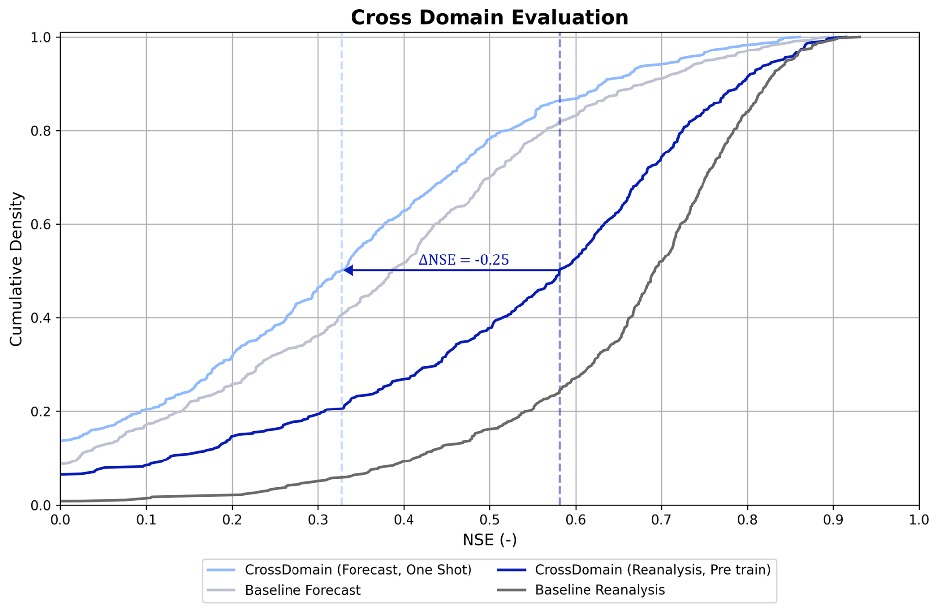
Figure 3 Cumulative Density Function of Nash Sutcliffe Efficiency values for the Cross Domain Evaluation Experiment. The comparison includes the Pre trained model on five meteorological reanalysis variables (dark blue), the One Shot (direct application without fine-tuning) based on the weights of the Pre trained model applied to the corresponding five meteorological forecasting variables from ECMWF-HRES and the baselines (grey). The vertical dashed lines depict the median NSE for each experiment. The blue arrow shows the performance decrease at median NSE when applying cross domain evaluation.

The underlying cause of this performance decrease can be attributed to the difference in data distributions between reanalysis and forecast datasets (see Appendix B), effectively representing a domain shift problem. Domain shift occurs when the statistical properties of the training data (reanalysis) differ from those of the target data (forecast), violating the fundamental assumption of independent and identically distributed data that underlies machine learning model generalization (Goodfellow et al., 2016; Hosna et al., 2022). Neural networks are particularly susceptible to domain shifts as they learn to map input-output relationships based on the specific distributional characteristics of their training data, leading to degraded performance when deployed on data from a different distribution. These results demonstrate that it is not feasible to simply substitute reanalysis data with forecast data in neural network-based hydrological modeling applications, as meteorological forecast uncertainty propagates through the model chain, degrading the representation of catchment processes and creating performance risks for operational hydrological forecasting systems.

Linking Meteorological Domain Shift to Topographical Features

Having established that the performance degradation in the cross-domain evaluation is driven by distributional differences between reanalysis and forecast inputs, we now investigate where across the 451 basins these differences are largest and which catchment characteristics are associated with larger domain shifts.

The Spearman correlation between the per-basin 1-Wasserstein distances and the 33 static catchment attributes reveals consistent patterns across all five meteorological variables, as shown in Fig. 4. Elevation-related attributes emerge as a strong and consistent predictor of domain shift across all variables, with mean elevation showing positive correlations ranging from r=0.19 (dewpoint temperature) to r=0.67 (precipitation), indicating that high-elevation catchments experience consistently larger distributional differences between reanalysis and ECMWF-HRES. This pattern is physically plausible, as ECMWF-HRES forecast skill is generally lower in complex alpine terrain where orographic effects are difficult to resolve at the model resolution (Haiden et al., 2024; Lavers et al., 2021).

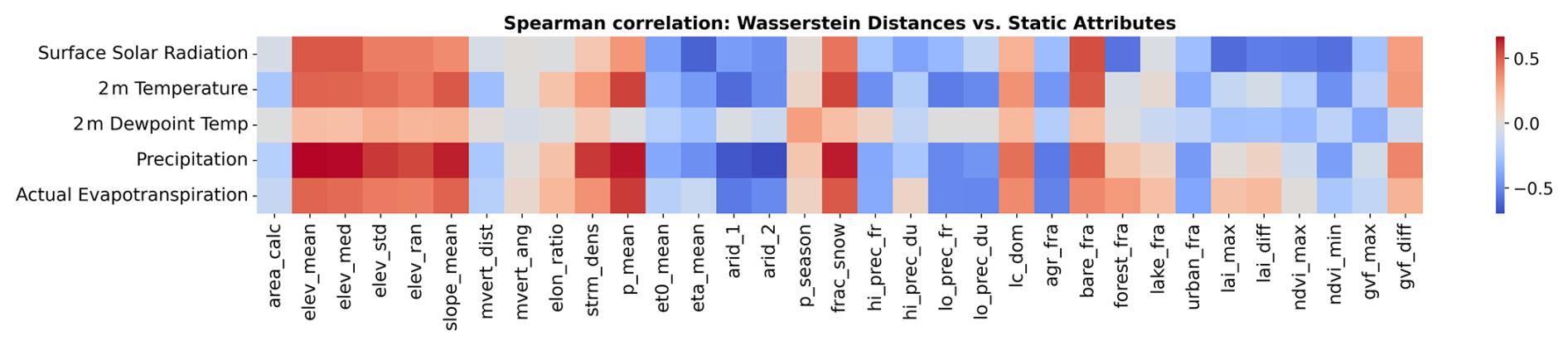
Figure 4 Spearman correlation between the per-basin 1-Wasserstein distances of five shared meteorological variables (Surface Solar Radiation, 2 m Temperature, 2 m Dewpoint Temperature, Precipitation, Actual Evapotranspiration) and 33 static catchment attributes across all 451 basins during the test period (2014–2017). Positive values (red) indicate that catchments with larger values of a given attribute tend to experience larger distributional differences between ERA5-Land reanalysis and ECMWF-HRES forecast inputs, while negative values (blue) indicate smaller distributional differences. Wasserstein distances are computed in the original physical units of each variable using the domains from the cross-domain evaluation experiment.

For surface solar radiation, the strongest positive correlation is found with bare fraction (r=0.54) and mean elevation (r=0.51), while the strongest negative correlation is with mean actual evapotranspiration ($r=-\mathrm{0.63}$) and LAI maximum ($r=-\mathrm{0.60}$), indicating that vegetated, low-elevation catchments with high evapotranspiration experience the smallest domain shift for this variable. For precipitation, mean elevation (r=0.67) and slope mean (r=0.63) show the strongest positive correlations, while aridity index shows the strongest negative correlation ($r=-\mathrm{0.66}$), suggesting that steeper, higher-elevation and wetter catchments experience larger distributional differences between the two precipitation products. For temperature, aridity index shows the strongest negative correlation ($r=-\mathrm{0.60}$), indicating that wetter catchments experience larger distributional differences between the two products, consistent with the positive correlations found for mean precipitation (r=0.57), fraction of snow (r=0.56) and slope mean (r=0.52), which are positively associated with wetter and more topographically complex conditions. For dewpoint temperature, correlations are substantially weaker across all attributes, with precipitation seasonality (r=0.31) and vegetation-related attributes such as GVF maximum ($r=-\mathrm{0.38}$) emerging as the dominant controls. For actual evapotranspiration, mean precipitation (r=0.58) and fraction of snow (r=0.52) show the strongest positive correlations, while aridity index ($r=-\mathrm{0.55}$) and agricultural fraction ($r=-\mathrm{0.53}$) show the strongest negative correlations, again suggesting that agriculturally dominated and drier catchments experience smaller domain shifts.

Overall, the results consistently indicate that topographically complex, high-elevation, snow-dominated catchments experience the largest distributional differences between reanalysis and forecast inputs, while low-elevation and vegetated catchments show smaller domain shifts.

3.2 Performance Analysis Across Unmodified Architectures

To address the domain shift challenges identified in Sect. 3.1, we evaluated different neural network architectures and training techniques, presenting here the optimal configurations from each experimental setup.

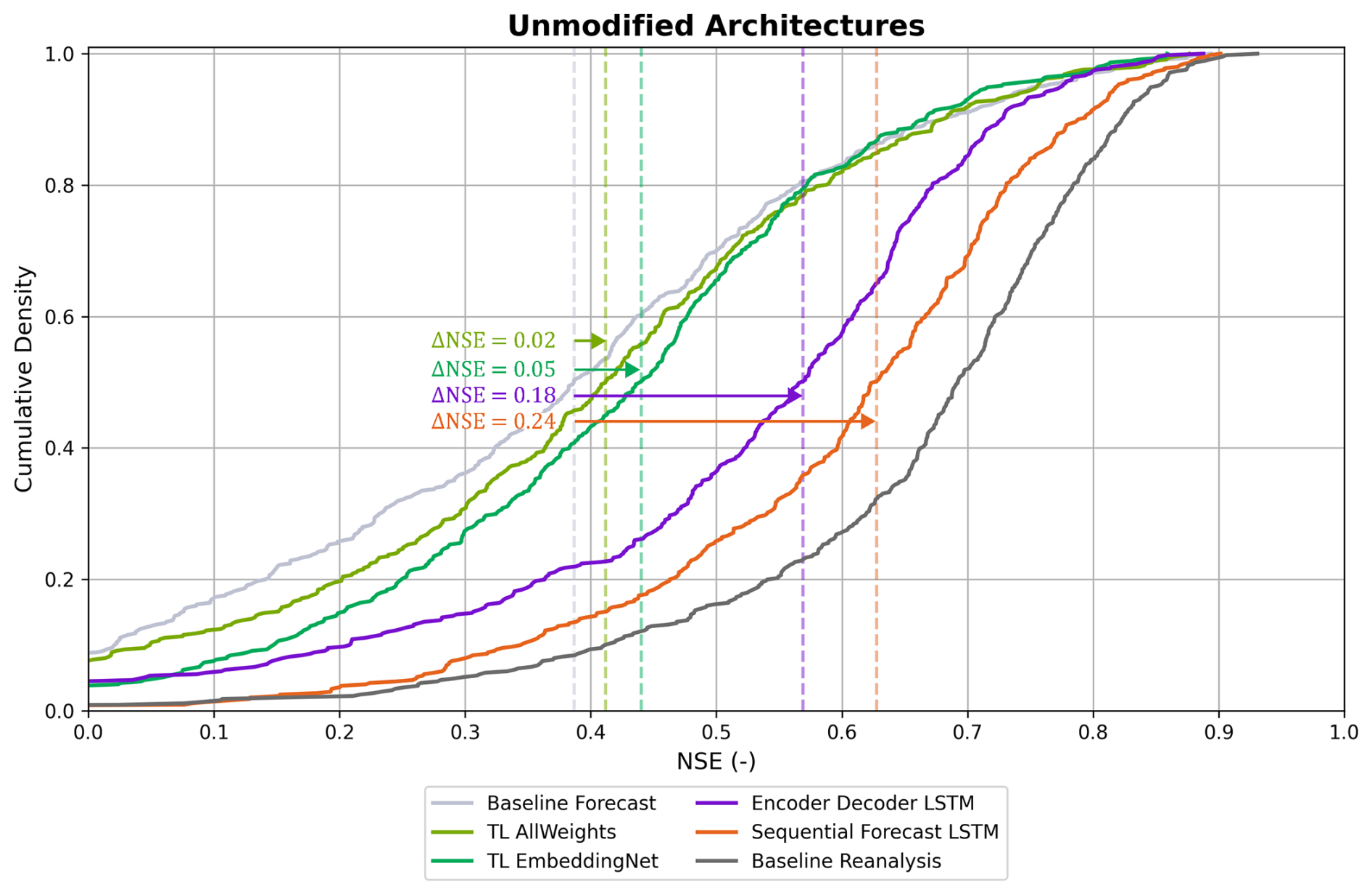
Figure 5 Cumulative Density Function of Nash Sutcliffe Efficiency values for the Unmodified Architectures Experiment. The experiments include the baselines (grey), comprehensive transfer learning with a finetuning of the embedding and LSTM weights (TL AllWeights), selective transfer learning with only finetuning the embedding weights while the LSTM was frozen (TL EmbeddingNet), Encoder- Decoder LSTM (purple) and the Sequential Forecast LSTM (orange). The vertical dashed lines depict the median NSE for each experiment. The arrows indicate the change in median NSE values relative to the baseline forecast experiment.

Transfer learning was implemented through two contrasting approaches: comprehensive parameter updating, where the entire network was retrained on forecast data (TL AllWeights), and selective embedding retraining, where only the input embedding layers were fine-tuned while maintaining the pre-trained weights of the deeper network components (TL EmbeddingNet). Both experiments utilized the reanalysis baseline with a complex embedding layer as the starting point. The selective embedding approach (TL EmbeddingNet) achieved higher performance, with a median NSE of 0.44, representing a 0.11 improvement over the cross-domain baseline (0.33). The advantage of selective retraining becomes evident when comparing the two transfer learning strategies: TL EmbeddingNet shows an improvement in the 10th percentile (0.15) compared to TL AllWeights (0.05), indicating that the retraining approach is especially effective for poorly performing basins. The enhanced performance stems from the model's ability to leverage robust hydrometeorological relationships learned from reanalysis data while adapting the input representation to forecast data characteristics. Reanalysis products provide more complete and physically consistent atmospheric descriptions through data assimilation, enabling the model to learn generalized process representations that are subsequently refined during fine-tuning on forecast data.

The Encoder–Decoder LSTM architecture demonstrated performance improvements over the transfer learning approaches, achieving a median NSE of 0.57. This architecture showed particular strength in the upper performance range, with the 75th and 90th percentiles reaching 0.65 and 0.73, respectively.

The Sequential Forecast LSTM achieved the highest overall performance among the unmodified forecast-based configurations, with a median NSE of 0.63 and notably consistent results across all percentiles. The model demonstrated higher stability compared to other approaches, evidenced by the low standard deviation (0.52). Among the unmodified architectures, the Sequential LSTM is best able to efficiently reduce forecasting bias. We attribute this to its two-phase processing structure, where the hindcast and forecast phases are processed consecutively within the same LSTM, maintaining a single continuous state evolution from hindcast to forecast. The cell state serves as long-term memory that can selectively retain or forget information across time steps, while the hidden state captures current relevant information, enabling the model to maintain both short-term adaptations to recent forecast patterns and long-term memory of systematic biases. Unlike the Encoder- Decoder architecture transforming hindcast states through a fixed handoff network before initiating forecast processing, the Sequential LSTM maintains continuous state evolution from hindcast to forecast, preserving temporal patterns without disruption and potentially enabling better compensation for systematic errors that emerge at the forecast transition.

3.3 The role of integrating archived forecasts in the hindcast phase

Given the performance degradation observed when transitioning from reanalysis to forecast data, we investigated whether training models with a combination of reanalysis and archived forecast data could improve forecast performance. In short, the integration of archived forecasts in the hindcast phase demonstrates limited effectiveness across all tested architectures.

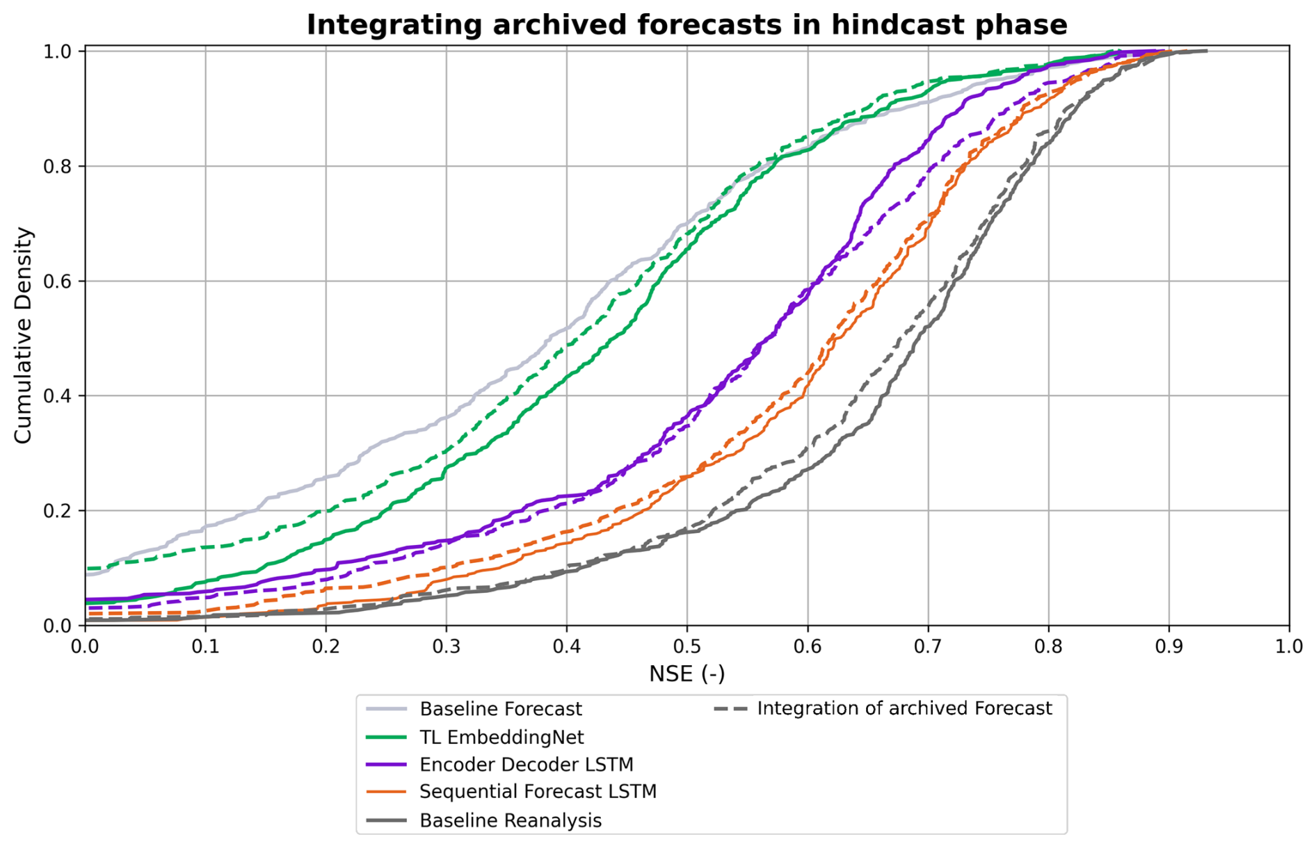
Figure 6 Cumulative Density Function of Nash Sutcliffe Efficiency values for experiments integrating archived forecasts in the hindcast phase. The experiments include the baselines (grey), selective transfer learning with only finetuning the embedding weights while the LSTM was freezed (TL EmbeddingNet), Encoder- Decoder LSTM (purple) and the Sequential Forecast LSTM (orange). Solid lines indicate the experiments with solely reanalysis data in the hindcast phase, while dashed lines display the combination of archived forecasts and reanalysis in the hindcast phase.

In Fig. 5 it is evident that in transfer learning only fine-tuning the embedding net led to higher forecast skill, leading us to only focus in this experimental setup on the selective transfer learning method. As previously discussed, the TL EmbeddingNet approach pretrained exclusively on reanalysis data achieved a median NSE of 0.44. In contrast, when the same transfer learning architecture is pretrained on combined forecast and reanalysis data, the results show deteriorated performance compared to the reanalysis-only pretraining, with a median NSE dropping to 0.41. This configuration exhibits increased variability (NSE standard deviation of 2.29) while the 10th percentile performance remains poor at 0.02, failing to achieve the improvement (0.15) observed with reanalysis-only pretraining. The mean performance also deteriorates significantly (0.21 vs. 0.35 for reanalysis-only), indicating the introduction of more negative outliers.

For the Encoder–Decoder LSTM, incorporating archived forecasts yields marginal improvements in the upper performance percentiles, with the 75th and 90th percentiles increasing from 0.65 to 0.69 and 0.73 to 0.77, respectively, while the 10th percentile improves slightly from 0.21 to 0.24. However, these modest gains are accompanied by increased variability (standard deviation increases from 8.03 to 9.33) while the median NSE remains unchanged at 0.57.

The Sequential Forecast LSTM shows no meaningful benefit from archived forecast integration, with the median NSE decreasing marginally from 0.63 to 0.62. More critically, this architecture experiences an increase in variability (standard deviation from 0.52 to 6.28) and the mean performance drops from 0.57 to 0.19, indicating the introduction of numerous extreme negative outliers that significantly compromise model reliability. A systematic explanation for these outliers has not been identified, but individual inspection of specific basins suggests that residual anthropogenic influences may play a role. For example, Basin 758 shows a persistent and strong overestimation of simulated discharge relative to observations throughout the test period, which is consistent with the presence of water abstractions, retention structures, or other human interventions not represented in the model. Despite filtering the 451 basins for low anthropogenic influence based on the LamaH-CE catchment classification, some residual human influence cannot be excluded.

The results demonstrate that integrating archived forecasts during the hindcast phase does not provide meaningful performance improvements for either architecture. The approach either yields negligible benefits while increasing instability (Encoder–Decoder LSTM) or actively degrades performance (Transfer learning, Sequential LSTM), indicating that this strategy is not effective for addressing domain shift challenges in hydrological forecasting applications.

3.4 The role of integrating past discharge in the training domain

Previous studies have consistently focused on modeling ungauged basins (Kratzert et al., 2019b; Nearing et al., 2024). However, we argue that when near real-time discharge data are available, as is the case for most gauging stations across the LamaH catchments in Central Europe, the incorporation of discharge observations positively influences forecast accuracy. For example, in the Austrian LamaH basins, discharge data from the eHYD platform (https://ehyd.gv.at, last access: 19 January 2026) are available with a time delay of only 2 h, making the integration of recent discharge observations operationally feasible for real-time forecasting applications.

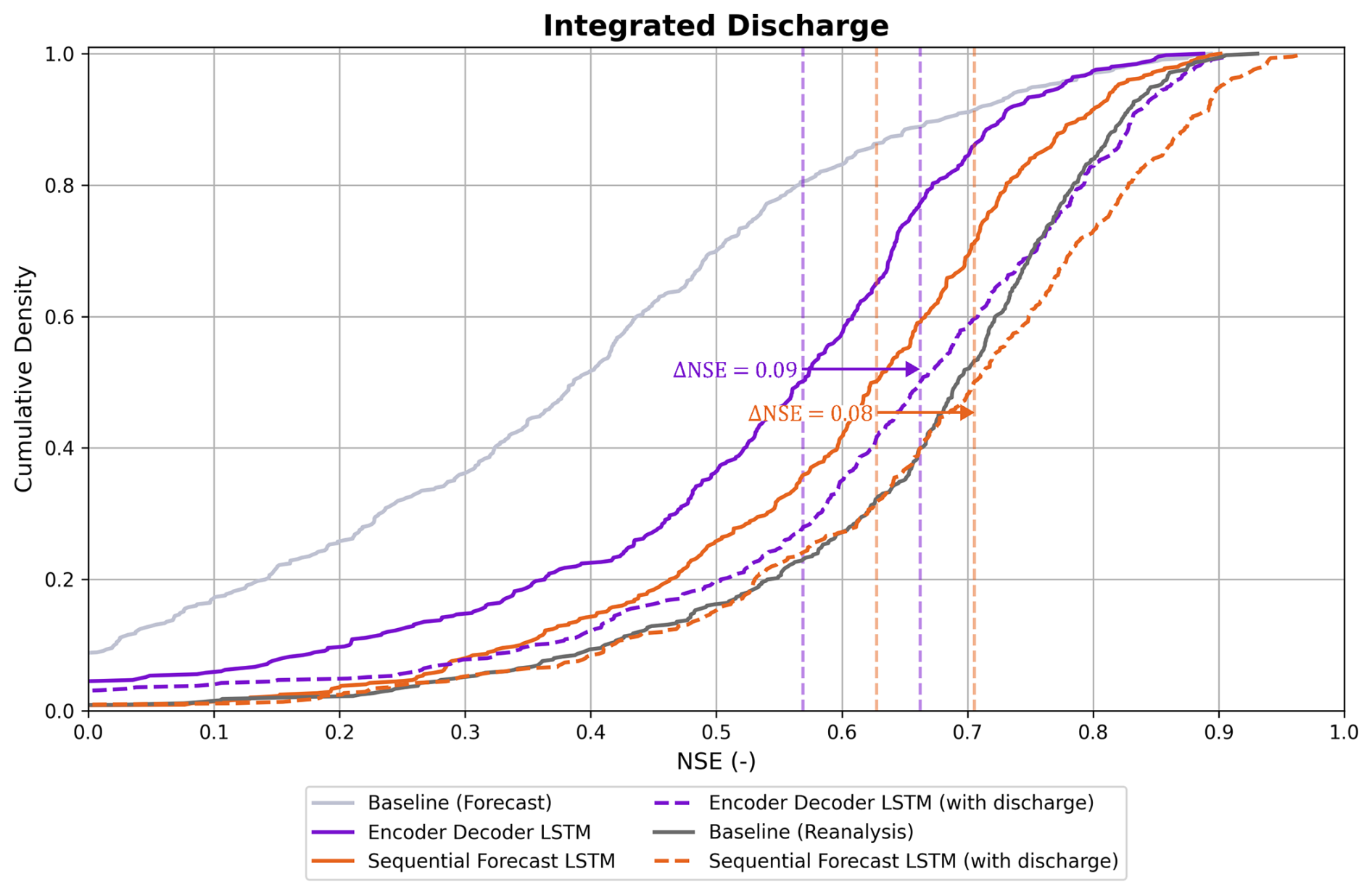
Figure 7 Cumulative Density Function of Nash Sutcliffe Efficiency values for experiments integrating past discharge in the hindcast phase. The experiments include the baselines (grey), Encoder- Decoder LSTM (purple) and Sequential Forecast LSTM (orange). Solid lines depict the experiments without discharge, while the dashed lines show experiments with discharge in the hindcast phase. The arrows represent the prediction accuracy increase as median ΔNSE when integrating discharge in the hindcast phase of the models.

The integration of past discharge observations demonstrates performance improvements across both tested architectures. For the Encoder–Decoder LSTM, incorporating discharge data yields significant gains, with the median NSE increasing from 0.57 to 0.66. The improvement is particularly pronounced in the lower percentiles, with the 10th percentile rising from 0.21 to 0.37, indicating considerably better performance for poorly performing basins. The 75th and 90th percentiles also show notable improvements (0.65 to 0.77 and 0.73 to 0.83, respectively), while the variability decreases slightly (standard deviation from 8.03 to 6.68).

When discharge is integrated, the Sequential Forecast LSTM achieves a median NSE of 0.71, compared to 0.63 without discharge. The absolute improvement (+0.08) is marginally smaller than for the Encoder–Decoder LSTM (+0.09), but the Sequential Forecast LSTM reaches a higher absolute performance level, surpassing even the reanalysis baseline of 0.69. The 10th percentile shows substantial improvement (0.35 to 0.42), while the upper percentiles reach 0.81 and 0.88 for the 75th and 90th percentiles, also exceeding the reanalysis baseline performance in these ranges.

The performance gains from discharge integration are not surprising given that near-real-time discharge observations constrain the current hydrological state through autoregressive inputs (Nearing et al., 2022), providing the model with direct information about catchment conditions at the time of forecast initialization that meteorological inputs alone cannot capture. These gains therefore reflect a combination of effects: beyond reducing meteorological forecast-induced bias, improved hydrological state estimation directly contributes to forecast skill regardless of meteorological input quality.

Additional transfer learning experiments were conducted to investigate whether discharge information learned during pre-training could be effectively transferred to discharge-free operational scenarios. These experiments included domain adaption configurations where discharge was incorporated during the pre-training phase but excluded during fine-tuning, as well as setups using the Sequential Forecast LSTM with discharge in the source domain and without discharge in the target domain. All transfer learning approaches consistently resulted in performance deterioration and failed to yield improvements that would justify the computational overhead of the transfer learning process. While these experiments demonstrated that information extraction from LSTM cell states is feasible, the learned discharge-related representations could not adequately compensate for the absence of direct discharge observations during operational forecasting. The experiments with discharge incorporated directly into the training data consistently outperformed all transfer learning alternatives, indicating that real-time discharge integration provides irreplaceable benefits that cannot be effectively substituted through knowledge transfer mechanisms.

3.5 The role of embedding complexity

During experimenting we experienced that the embedding complexity plays an important role in reducing the forecast induced bias in runoff predictions. This circumstance has led us to create this experimental setup, in which a simple (linear) and a complex (non-linear) embedding were generated for all architectures used in the previous experimental settings. In brief, a similar pattern can be observed for all architectures except transfer learning: the more complex the input embedding, the lower the prediction performance.

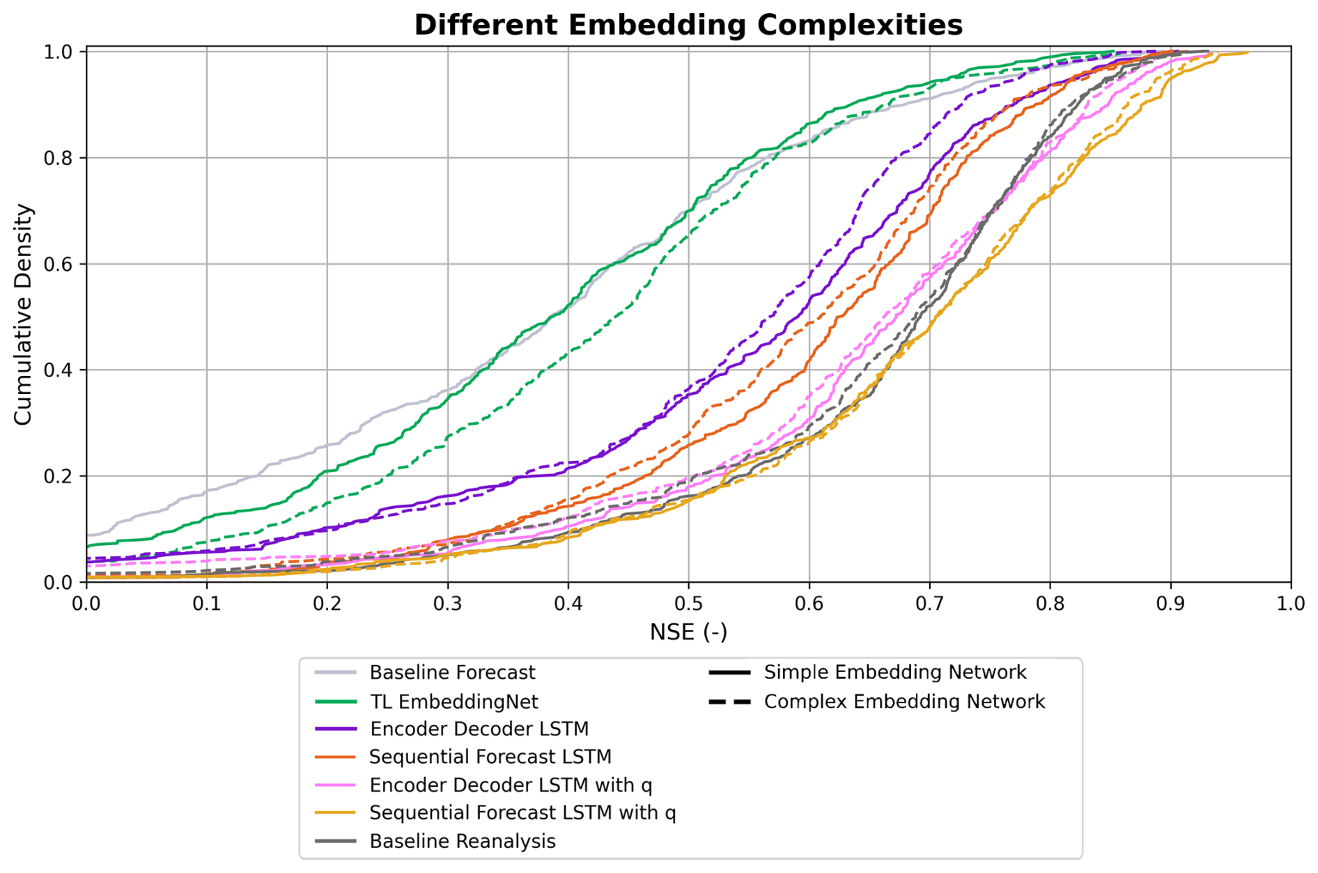
Figure 8 Cumulative Density Function of Nash Sutcliffe Efficiency values for experiments with different embedding complexities. The experiments include the baselines (grey), selective transfer learning with only finetuning the embedding weights while the LSTM was freezed (TL EmbeddingNet), Encoder–Decoder LSTM without discharge (purple), Encoder–Decoder LSTM with discharge (pink), Sequential Forecast LSTM without discharge (orange) and Sequential Forecast LSTM with discharge (yellow). Solid lines depict the experiments without simple linear embedding, while the dashed lines show experiments with complex non- linear embedding networks.

While the transfer learning experiments did not achieve the high NSE values of the best-performing forecasting approach (Sequential LSTM), notable relationships emerged between embedding complexity and prediction accuracy. In the baseline, encoder–decoder and sequential LSTM experiments, simple linear embedding networks produced slightly higher simulation performance compared to more complex embedding architectures. This pattern reversed in transfer learning experiments, where increased embedding complexity led to improved prediction results. The transfer learning procedure consisted of transferring weights from an LSTM model pre-trained on all available reanalysis data (𝒟_RA) to a new network architecture with modified input embeddings, where only the embedding weights underwent retraining while the remaining LSTM parameters remained frozen.

The minimal performance improvement of simple embeddings in non-transfer learning experiments can be attributed to the tendency of complex embedding networks to overfit when trained on the available data. The number of trainable parameters in complex embeddings exceeds the optimal ratio relative to available training data, causing the model to learn specific noise patterns in the training data rather than generalizable hydrological patterns. This overfitting tendency is further amplified by the absence of dropout regularization within the embedding networks, which was set to 0 across all experiments. Additionally, the use of tanh activations in both the embedding networks and the LSTM may compound saturation effects (Acuña Espinoza et al., 2025), potentially contributing to the performance degradation observed with more complex embeddings. This means simpler embeddings capture the relevant input patterns more effectively without introducing unnecessary model complexity comprising generalization.

The improved results with increased embedding complexity in transfer learning can be explained by the requirement for flexible, non-linear transformations necessary for effective domain adaptation. Since only the embedding weights are trained while all other network parameters remain frozen, the embedding layer must perform all adaptation work between the target domain and the representations pre-trained on reanalysis data. More complex architectures can perform richer and more domain-specific feature extraction, compensating for the discrepancy between source and target domains through more expressive input transformations. The contrasting performance patterns between transfer learning and standard training suggest that the optimal embedding complexity depends on whether the model parameters are trained from scratch or adapted from pre-trained weights, though the precise mechanisms underlying this relationship warrant further investigation.

3.6 Physiographic Controls on Model Skill

While the previous sections demonstrated the overall effectiveness of the proposed bias correction strategies, a key operational question remains: does model skill improve uniformly across catchment types, or do specific basin characteristics such as aridity, elevation, land cover, or precipitation regime determine which catchments benefit most from the proposed strategies?

Inspired by the benchmark framework of Seibert et al. (2018), who argue that model performance should always be evaluated relative to meaningful reference points, we compute the per-basin ΔNSE between each experimental configuration from Sect. 3.2 and 3.4 to the Baseline Forecast. Figure 9 shows these ΔNSE values with basins sorted by their mean ΔNSE across all experiments in ascending order, providing a clear picture of which basins consistently improve, remain unchanged, or degrade in forecast skill across the proposed strategies.

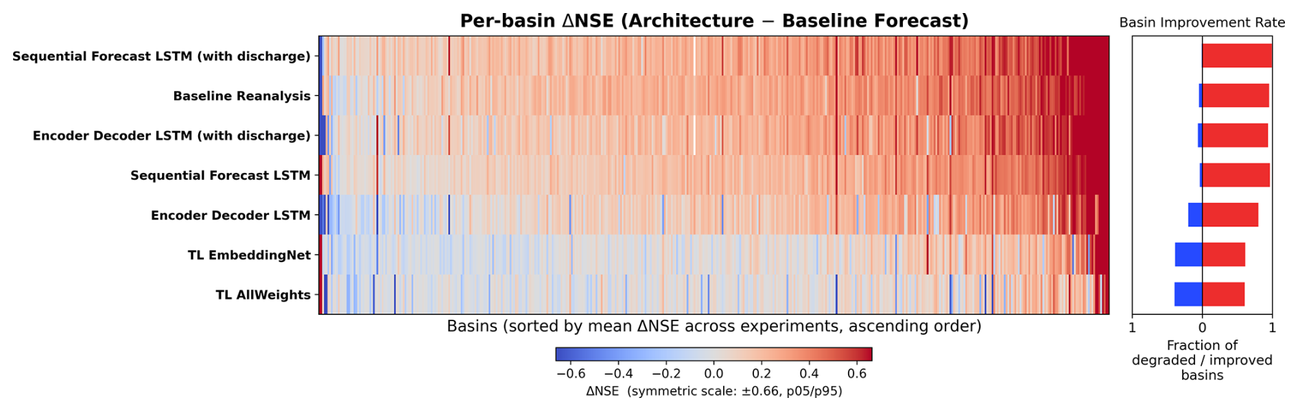
Figure 9 Per-basin skill difference (ΔNSE) between each model architecture and the Forecast Baseline across 451 gauged catchments of the LamaH-CE dataset. Each row corresponds to one experiment and each column to one catchment. ΔNSE is defined as the difference between the basin NSE values from an architecture (rows) and the Baseline Forecast, where positive values (red) indicate that the architecture outperforms the baseline and negative values (blue) indicate degraded performance. Basins are sorted left to right by their mean ΔNSE across all experiments (ascending), and experiments are sorted top to bottom by their median ΔNSE (descending). The colour scale is symmetric and bounded by the 5th and 95th percentiles of the pooled ΔNSE distribution. The bar chart on the right shows the fraction of catchments with improved (red) and degraded (blue) performance relative to the baseline for each experiment.

The results in Fig. 9 reveal that the Sequential Forecast LSTM with discharge integration achieves positive ΔNSE values across the vast majority, with 445 of the 451 basins, confirming that nearly all basins benefit from this configuration relative to the Baseline Forecast. A small number of isolated basins show exceptionally large positive ΔNSE values, visible as dark red columns, which are particularly pronounced in the discharge-augmented configurations and likely reflect basins where near real-time discharge observations provide especially strong anchoring of the initial hydrological state. The Baseline Reanalysis shows a very similar basin-level improvement pattern, consistent with its role as the upper performance reference.

A clear and consistent architectural difference emerges between the Sequential Forecast LSTM and the Encoder–Decoder LSTM. The Sequential Forecast LSTM without discharge integration already improves 435 out of 451 basins, while the Encoder–Decoder LSTM without discharge improves only 361 out of 451 basins and actively degrades 90, nearly 5 times as many as the Sequential Forecast LSTM. Even with discharge integration, the Encoder–Decoder LSTM degrades 28 basins compared to only 5 for the Sequential Forecast LSTM. This persistent instability is consistent with the higher standard deviations reported for the Encoder–Decoder architecture in Sect. 3.2 and suggests that the fixed handoff network introduces fragility for specific basin conditions that the Sequential LSTM's continuous state evolution avoids.

The transfer learning configurations show the most heterogeneous basin-level patterns. TL EmbeddingNet and TL AllWeights improve only 275 and 273 out of 451 basins respectively, while degrading the rest, indicating that both transfer learning strategies fail to provide consistent improvements across the basin population and cannot be considered reliable bias correction strategies across diverse catchment conditions.

Since we now know which catchments benefit most from each architecture in terms of increased forecasting skill, we further investigate which catchment characteristics determine where the largest improvements occur. To this end, we focus exclusively on basins with positive ΔNSE values (red columns in Fig. 9) – that is, basins where the proposed strategy outperforms the Baseline Forecast. Basins with negative ΔNSE are excluded from this analysis. Figure 10 shows the Spearman correlation between the per-basin ΔNSE and the 33 static catchment attributes across all experimental configurations for this subset of basins. Positive values indicate that catchments with larger values of a given attribute tend to benefit more from the proposed strategy, while negative values indicate smaller improvements.

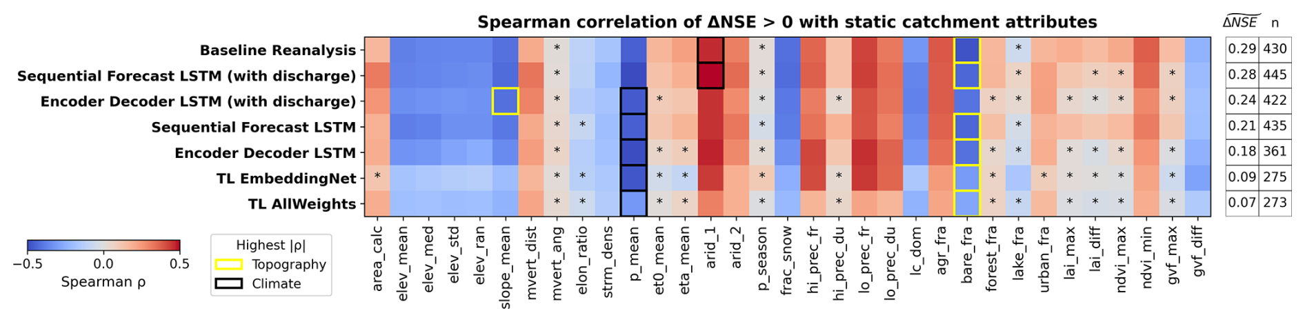
Figure 10 Spearman correlation of experiments with improved model skill compared to the Forecast Baseline, denoted as ΔNSE >0. Each row corresponds to one experiment and each column to a static catchment attribute used in model training. The Asterisk shows the non significant attributes (p>0.05).

The Spearman correlation between per-basin ΔNSE and static catchment attributes reveals a consistent and striking pattern across all experimental configurations. Aridity index (arid_1) and mean precipitation (p_mean) emerge as the dominant controls on the magnitude of improvement, with aridity showing positive correlations across all experiments (ranging from r=0.31 for TL AllWeights to r=0.50 for the Sequential Forecast LSTM with discharge) and mean precipitation showing consistently negative correlations of similar magnitude ($r=-\mathrm{0.31}$ to $r=-\mathrm{0.50}$). This indicates that drier catchments benefit more from the proposed bias correction strategies in absolute terms, while wetter catchments show smaller improvements over the Baseline Forecast.

When combined with the Wasserstein distance analysis of Sect. 3.1.1, these results reveal a physically meaningful asymmetry. The attributes showing larger meteorological domain shift between reanalysis and forecast inputs, including mean precipitation, mean slope, fraction of snow and aridity, are precisely the same attributes associated with smaller improvements in forecast skill across all experimental configurations. Conversely, the basins associated with smaller meteorological domain shift, characterized by higher aridity and more frequent dry days, are the same associated with larger gains in forecast skill relative to the Baseline Forecast (see Fig. 11). We explain this paradox by the nature of the hydrological signal in different catchment types: alpine, wet, and snow-dominated catchments experience the largest distributional differences between reanalysis and ECMWF-HRES inputs, but their hydrology is dominated by a strong and seasonally predictable snowmelt signal. This signal is captured and retained in the LSTM cell state through its recurrent processing of the 365 d input sequence, enabling the model to compensate for the large meteorological domain shift through its long-term memory mechanism even when forecast inputs are strongly biased. This interpretation is consistent with the findings of Kratzert et al. (2019a), who demonstrated that LSTM memory cells internally learn to represent snow storage dynamics even without snow being explicitly provided as a model input, confirming the ability of LSTMs to encode physically meaningful hydrological states in their cell states. As a result, even the Baseline Forecast achieves relatively good performance in alpine catchments, leaving less room for improvement from the proposed strategies. In contrast, drier and more episodic catchments experience smaller meteorological domain shifts but have weaker and more nonlinear rainfall-runoff relationships that are more sensitive to input quality, leading to lower Baseline Forecast performance and consequently larger absolute improvements when different model architectings or training strategies are applied.

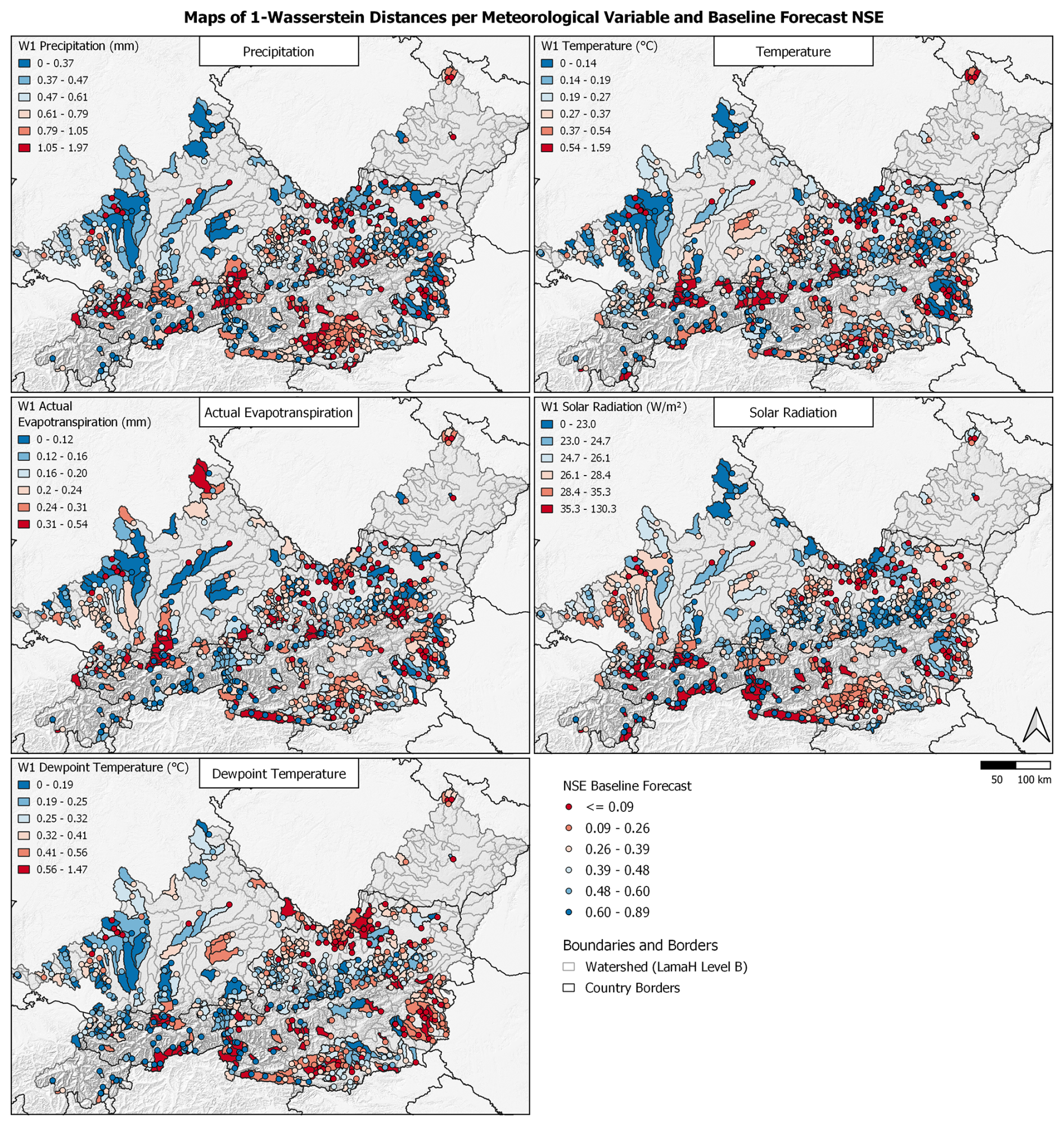
Figure 11 Maps of the 1-Wasserstein distance between Reanalysis and ECMWF-HRES Forecast distributions for five meteorological variables (Precipitation, Temperature, Actual Evapotranspiration, Solar Radiation and Dewpoint Temperature) across the 451 LamaH basins during the test period (2014–2017), shown as basin polygons colored by Wasserstein distance. Gauge locations are overlaid as circles colored by the per-basin NSE of the Baseline Forecast experiment, providing a direct spatial comparison between the magnitude of meteorological domain shift and the model skill achieved without any bias correction strategy. Larger Wasserstein distances indicate greater distributional differences between the two data products at a given basin.

This finding has important operational implications. While the proposed strategies consistently outperform the Baseline Forecast across the vast majority of basins as shown in the CDFs, the largest absolute gains are concentrated in arid catchments where the hydrological response is more complex and the baseline performance is lowest, rather than in the topographically complex alpine catchments where the meteorological input bias is largest.

3.7 Limitations and Future Directions

This study is subject to several limitations. The experiments were conducted on the Extended LamaH-CE dataset, which is restricted to Central Europe; the transferability of the results to other hydroclimatic regions remains to be tested. While discharge observations were shown to substantially improve performance, they are not error-free, and their availability cannot be guaranteed in ungauged or poorly monitored catchments. The focus on a 1 d lead time restricts the conclusions that can be drawn regarding forecast quality decay with increasing lead time, and extension to multi-day-ahead forecasting is the subject of a forthcoming study.

In addition, we only evaluated existing LSTM-based architectures and a modeling setup with spatially lumped data and daily maximum discharges. Applying these approaches in fully distributed settings with higher temporal resolution forecasts may yield different, potentially more pronounced results.

The use of ECMWF-HRES as the only forecast dataset was driven by data availability – to our knowledge, ECMWF-HRES is the only NWP system for which sufficiently long archives of forecast data are openly available to cover the experimental period used in this study. From a theoretical standpoint, however, the approach is not inherently tied to any specific NWP system. A key advantage of using discharge as the target variable is that the model trains on an integrated catchment signal that implicitly captures the combined effect of all meteorological inputs, regardless of their source, meaning the training strategy can in principle be applied to any NWP system by replacing or supplementing the forecast inputs accordingly. Drawing on the findings of Kratzert et al. (2021), who demonstrated that combining multiple meteorological data sources improves LSTM simulation accuracy in a reanalysis setting, we further hypothesize that combining forecasts from multiple NWP systems could yield similar benefits in a forecasting context, enabling the model to learn source-specific bias patterns and potentially improving robustness across different forecast systems

The integration of reanalysis data in the hindcast phase, while useful for training, is also constrained by data latency, which is often critical for operational use, although future improvements in near–real-time reanalysis may alleviate this. However, this limitation depends strongly on the application scale. At national scales, real-time analysis, nowcast, or station-based observed data can serve as the hindcast forcing, bypassing reanalysis latency entirely. Products such as INCA from GeoSphere Austria (Haiden et al., 2011) are a good example of operationally available high-resolution analysis data that could fill this role. In large-sample settings such as ours, however, station-based data could introduce further practical challenges, as the number of stations per basin varies greatly, a large basin may contain dozens of stations while a small one may have only one, complicating consistent spatial aggregation and resulting in varying input dimensions across basins. While input embeddings as used in this study could potentially help map these varying input dimensions into a shared latent space, the implications for model performance and stability in such a setting remain an open question.

Addressing these challenges – testing transferability, reducing dependence on delayed or unavailable inputs, and extending both the spatial and temporal resolution of experiments – will be essential to further investigate and advance robust, operationally viable solutions for flood forecasting.

4 Conclusion and Outlook

The operational deployment of deep learning based flood forecasting models faces fundamental challenges when transitioning from high-quality reanalysis to meteorological forecast data, with domain shift between these data sources leading to model performance degradation. While previous approaches have focused on bias-correcting meteorological inputs through statistical methods (Lenderink et al., 2007) or machine learning techniques applied to precipitation forecasts (Ko et al., 2020; Zhang et al., 2020), these methods rely on comparing forecasts with meteorological observations that themselves contain uncertainties (Bárdossy et al., 2022). This study addressed the challenge through systematic evaluation of Long Short-Term Memory architectures and training techniques that learn bias correction directly from the more reliable discharge observations, following the paradigm suggested by Kirchner (2009) of using river discharge as the primary constraint. Our experiments across 451 Central European catchments demonstrated that appropriate neural network designs can transform the domain shift problem from a major obstacle into a learnable pattern correction task. Sequential Forecast LSTM architectures, when combining meteorological hindcast data with past discharge observations, provided the most effective framework for mitigating forecast-induced biases. This configuration achieved a median NSE of 0.71, surpassing even the reanalysis baseline simulation and establishing discharge integration, if data are available in near real time as in the LamaH domain, as a critical component for operational forecast accuracy.

To quantify the bias propagation caused by the domain shift, we conducted cross-domain evaluation revealing performance deterioration when reanalysis-trained models were applied to forecast inputs. In this setting, the median Nash-Sutcliffe Efficiency decreased from 0.58 to 0.33, representing a 0.25 reduction in model skill. This performance degradation stems from fundamental differences in data distributions between reanalysis and forecast datasets, violating the assumption of identically distributed training and testing data that underlies machine learning model generalization (Goodfellow et al., 2016). Analysis of the spatial patterns of this input data domain shift, quantified using the 1-Wasserstein distance across the 451 basins, reveals that topographically complex, high-elevation, and snow-dominated catchments experience the largest distributional differences between reanalysis and ECMWF-HRES inputs, potentially driven by the limited ability of numerical weather prediction models to resolve orographic effects at their operational resolution (Haiden et al., 2024; Lavers et al., 2021).

Among the tested neural network architectures, the Sequential Forecast LSTM demonstrated superior performance for operational forecasting applications. This architecture achieved a median NSE of 0.63 with notable stability (standard deviation of 0.52) and maintained reasonable performance across all percentiles. The sequential processing approach enables gradual correction of forecast biases through continuous state evolution from hindcast to forecast phases, preserving temporal patterns without the disruption introduced by fixed handoff networks in Encoder–Decoder architectures. Transfer learning approaches, despite theoretical advantages for domain adaptation, achieved only modest improvements (NSE 0.44), while the incorporation of archived forecasts in training failed to provide consistent benefits and often increased model instability. The relationship between embedding complexity and performance varied systematically: simpler embeddings performed better in standard training contexts, while complex embeddings showed advantages only in transfer learning scenarios where flexible input transformations were required for domain adaptation.

These findings carry important implications for operational flood forecasting system design. The high performance of Sequential Forecast LSTM architectures indicates that operational systems should prioritize continuous state transfer mechanisms maintaining temporal dependencies across the hindcast-forecast phases rather than treating these phases as disconnected processes. The improvements from discharge integration are consistent with the operational capabilities of many monitored systems, such as hydro power plants or the Austrian eHYD platform, where observations are available with a minimal latency, making real-time integration feasible. The ability to learn bias correction patterns directly from the combined meteorological-hydrological data space eliminates the need for separate pre-processing steps, whether meteorological bias correction (Hess, 2020; Han et al., 2021) or streamflow post-processing methods like the approach of Hunt et al. (2022), reducing computational overhead and possibly potential error propagation. Basin-level analysis of forecast skill improvements, measured as the difference in NSE between each tested architecture and the Baseline Forecast, reveals that the proposed strategies do not improve performance equally across catchment types. While the Sequential Forecast LSTM with discharge integration outperforms the Baseline Forecast in 445 out of 451 basins, the magnitude of improvement varies systematically with catchment characteristics. The largest absolute gains are concentrated in arid and precipitation-limited catchments, where weaker and more nonlinear rainfall-runoff relationships make model skill more sensitive to input quality. In contrast, alpine and snow-dominated catchments, despite experiencing the largest meteorological domain shift, show smaller improvements – a phenomenon we explain with the LSTM cell state capturing and retaining the strong seasonal snowmelt signal through its long-term memory mechanism, enabling effective compensation for forecast input bias even without explicit bias correction. Future developments should focus on adaptive architectures that can dynamically leverage discharge observations when available while maintaining robust performance in ungauged settings through reanalysis-only hindcast processing. Such unified frameworks would enable seamless deployment across both gauged and ungauged basins within the same operational system, automatically adjusting to data availability in real-time. However, sensor failures should also be taken into account here, and the training methods proposed by Gauch et al. (2025) should be applied. While our experiments were limited to ECMWF HRES archived forecasts due to data availability, combining multiple forecasts from different sources could also be promising as it could capture forecast uncertainty more comprehensively and enable the model to learn source-specific bias patterns, as with the integration of multiple meteorological data in a simulation setting (Kratzert et al., 2021). The Sequential Forecast LSTM's bias correction capabilities at 24 h lead times provide a strong foundation for multi-day forecasting applications, where learning lead-time dependent bias patterns could improve medium-range flood predictions that are crucial for early warning systems and emergency preparedness. The demonstrated ability of LSTM architectures and training techniques to transform the domain shift challenge into a learnable bias correction problem, combined with increasing availability of real-time hydrological observations, establishes a pathway toward operational flood forecasting systems that can maintain predictive skill despite the inherent uncertainties coming from numerical weather predictions. Beyond the methodological advances presented here, the spatially heterogeneous patterns of domain shift and forecast skill improvement identified across the 451 study basins open a promising avenue for future research: understanding why forecast-induced bias manifests differently across catchment types in terms of its temporal dynamics, physiographic controls, and physical mechanisms. This represents the natural next step toward a comprehensive theory of forecast uncertainty in data-driven hydrological modelling.

Appendix A: Dynamic and Static Forcings of the Models

Table A1 Meteorological Variables in the Extended LamaH-CE data set used for the conducted experiments. All reanalysis variables are used as dynamic inputs across all experiments, with two exceptions: the Cross Domain evaluation, where only the five variables with a direct equivalent in the ECMWF-HRES forecast data are used (see Table 1) to ensure an identical input feature space between training and inference; and the Baseline Forecast experiment, where only the five ECMWF-HRES forecast variables are used as dynamic inputs.

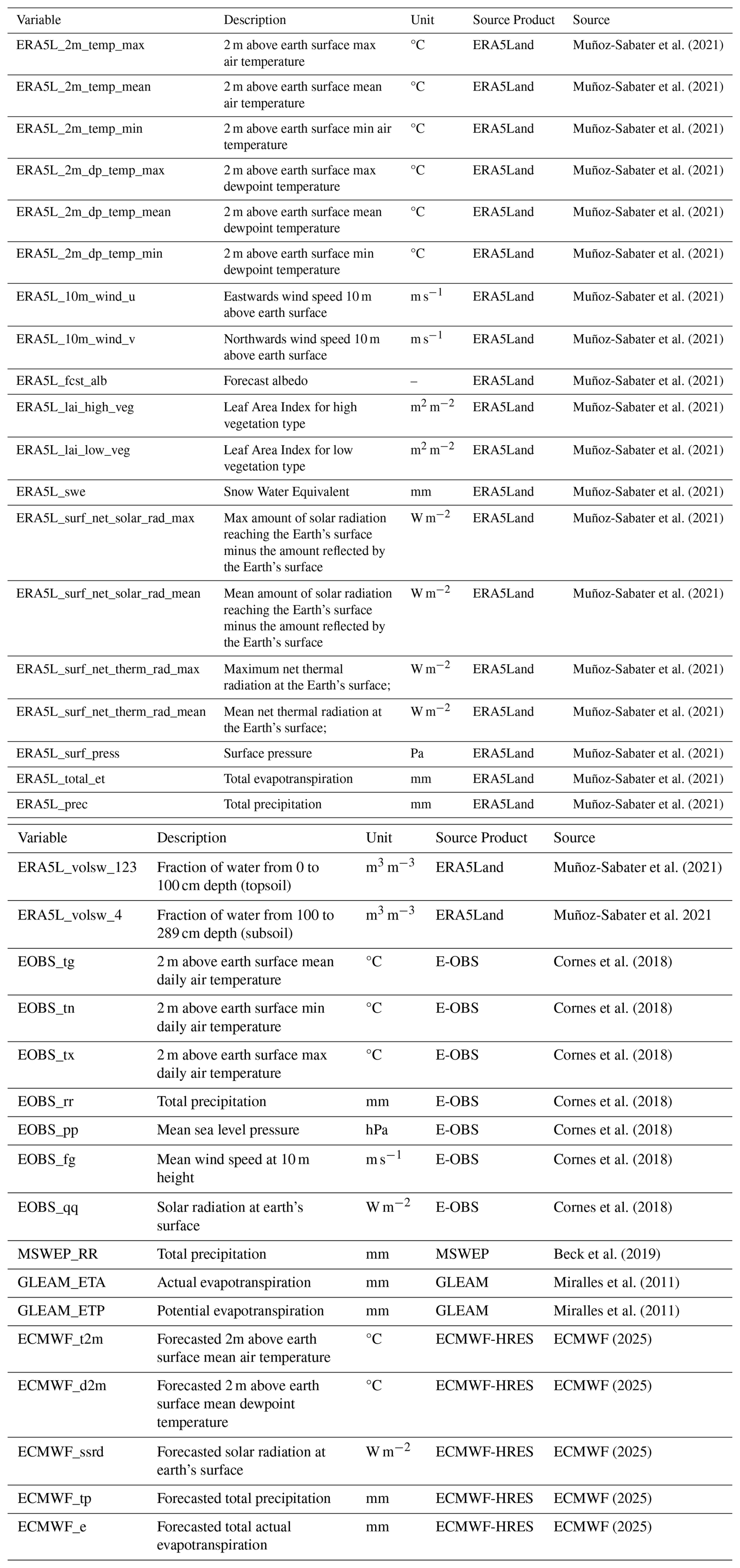
Table A2 Static catchment attributes from the Extended LamaH-CE data set used for the conducted experiments.

Appendix B: Variability across input data sets

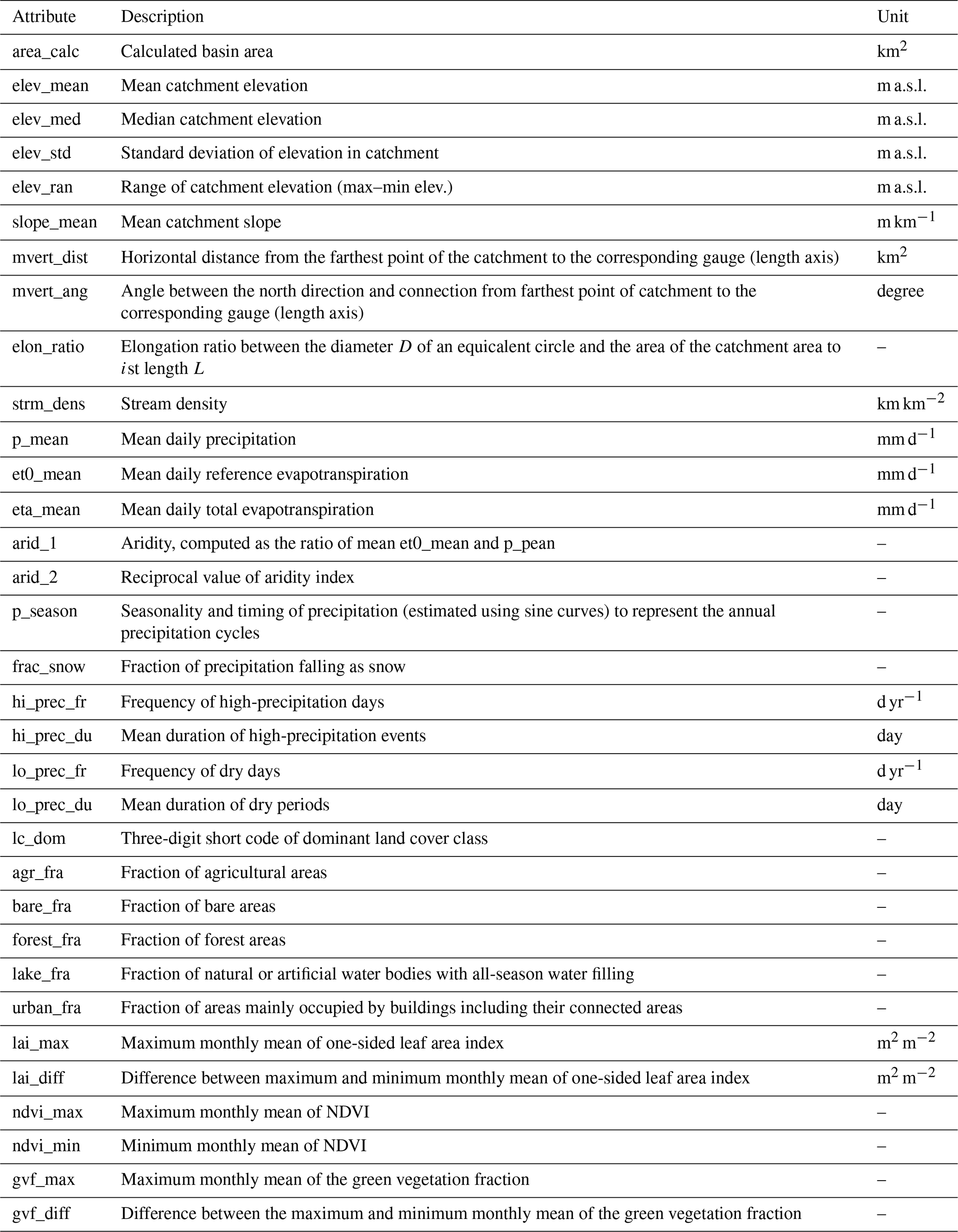
The violin plots in Fig. B1 show the distributions of annually aggregated meteorological variables across all data products and 451 basins. It should be noted that these distributions reflect annual aggregates, and differences at the daily resolution used in the experiments may deviate from the patterns shown here. For temperature and dewpoint temperature, ERA5-Land shows a wider spread than ECMWF-HRES, with ERA5-Land reaching lower minimum values, while the medians differ by less than 0.2 °C between the two products. For precipitation, ERA5-Land reports the highest median annual sum (1223 mm), while E-OBS and MSWEP report notably lower medians (1047 and 1119 mm respectively), with ECMWF-HRES falling in between (1175 mm). The most pronounced differences are found for solar radiation, where ECMWF-HRES reports a median annual sum approximately 11 000 W m⁻² higher than ERA5-Land, and ERA5-Land exhibits a substantially wider and lower-reaching distribution. For evapotranspiration, ERA5-Land and GLEAM show wider spreads with notably lower minimum values compared to ECMWF-HRES, while the medians differ by up to 29 mm annually. These distributional differences across all five variables collectively represent the domain shift that the models must learn to compensate for when transitioning from reanalysis to forecast inputs, as quantified by the 1-Wasserstein distances in Sect. 3.1.1.

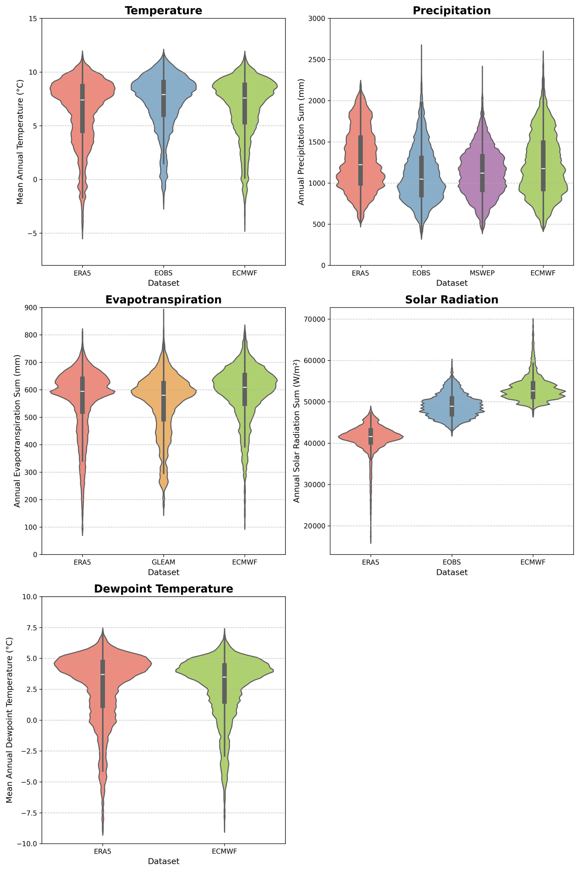
Figure B1 Variability across input data sets displayed as violin plots for annually aggregated meteorological variables Temperature, Precipitation, Actual Evapotranspiration, Solar Radiation and Dewpoint Temperature. The violin colours belong always to a certain data product: red- ERA5Land, orange: GLEAM, blue: E-OBS, green: ECMWF-HRES, purple: MSWEP. The dark grey box in the violin shows a boxplot with the bold part depicting the interquartile range and the white line indicating the median.

Appendix C: Evaluation Metrics

The model performance was evaluated by using the non basin specific NSE* of Kratzert et al. (2019c) which is based on the Nash and Sutcliffe Efficiency (NSE; Nash and Sutcliffe, 1970). In Eq. (C2), B is the number of basins, N is the number of days per basin B, $\widehat{y_n}$ is the predicted value for sample n, y_n is the corresponding observed value and s(b) is the training periods standard deviation of the discharge in basin b. For numerical stability, the term $\in =\mathrm{0.1}$ is added to the denominator. In comparison to former studies (Kratzert et al., 2019b, c, 2021; Nearing et al., 2024), we conducted no cross validation across spatial units, since we did not focus on ungauged basins. Instead, we employed a temporal split validation approach, where the available time series data for each catchment was divided into training, validation, and testing periods to ensure robust model evaluation.

$$\begin{array}{}\text{(C1)}& {\displaystyle }\mathrm{NSE}=\mathrm{1}-{\displaystyle \frac{\sum _{i=\mathrm{1}}^n{\left(y_{\mathrm{obs},i}-y_{\mathrm{sim},i}\right)}^{\mathrm{2}}}{\sum _{i=\mathrm{1}}^n{\left(y_{\mathrm{obs},i}-{\stackrel{\mathrm{‾}}{y}}_{\mathrm{obs}}\right)}^{\mathrm{2}}}}\text{(C2)}& {\displaystyle }\mathrm{NSE}*={\displaystyle \frac{\mathrm{1}}{B}}\sum _{b=\mathrm{1}}^B\sum _{n=\mathrm{1}}^N{\displaystyle \frac{(\widehat{y_n}-y_n{)}^{\mathrm{2}}}{\left(s\right(b)+\in {)}^{\mathrm{2}}}}\end{array}$$

Appendix D: Hyperparameter Optimization

Hyperparameter tuning is a critical component in the bias correction of meteorological forecasting data using Long Short-Term Memory (LSTM) networks, as it directly influences the model's ability to learn complex temporal patterns and correct systematic biases in forecast inputs. Given the nonlinear and dynamic nature of meteorological variables, appropriate selection of hyperparameters such as learning rate, sequence length, number of hidden units, dropout rate, and batch size, is essential to ensure that the LSTM model generalizes well without overfitting to noise or underfitting relevant signals. In the context of bias correction, the model must not only capture historical dependencies in the forecast errors but also effectively differentiate between genuine atmospheric variability and persistent model biases. Without careful tuning, the LSTM may fail to correct biases accurately, particularly under extreme events or seasonal transitions.

To this end, we used Bayesian optimization as described by Frazier (2018). This search algorithm fits a Gaussian process to the observed hyperparameter-performance pairs to estimate performance on yet-untested parameter settings. We use the expected improvement as acquisition function, which is used for selecting the next set of hyperparameters to test. This approach efficiently identifies good hyperparameters, especially in large search spaces.

For our models, we spanned the search space over the hidden layer sizes (64, 128, 256 units), output dropout rates (0.1, 0.2, 0.3), variance of Gaussian noise applied to the discharge values (0.001, 0.01, 0.1), and batch sizes (64, 128, 256) and limited the number of iterations to 100. To obtain the result for each setting, we trained a model for 30 epochs, an initial learning rate of 0.001 and a cosine annealing schedule (T_max = 30, η_min = $\mathrm{1}\times {\mathrm{10}}^{-\mathrm{5}}$), stopping early if the model did not improve the evaluation metric by more than 0.005 in the last 5 epochs. To estimate the performance of the model we used the basin averaged Nash-Sutcliffe efficiency (NSE*) metric and evaluated it on the validation period.

NSE* with hyperparameter optimization:

$$\begin{array}{}\text{(D1)}& \mathit{\lambda }=\arg \underset{\mathit{\lambda }}{\max }{\text{NSE}}_{\mathrm{median}}\left(D_{\mathrm{val}};\mathit{\lambda }\right)\end{array}$$

where

$$\begin{array}{}\text{(D2)}& \mathit{\lambda }=\mathit{\{}{d}_h,p_{\mathrm{dropout}},{\mathit{\sigma }}_{\mathrm{noise}},b_{\mathrm{size}}\mathit{\}}\end{array}$$

represents the optimal output.

Appendix E: Long-Short Term Memory Network

Long term information is stored in the cell state (c_t), short term information in the hidden state (h_t) and the information flow is controlled by the so- called gating mechanisms (Hochreiter and Schmidhuber, 1997). The input gate (i_t) determines how much of the current input and previous hidden state contributes to updating the cell state. The forget gate (f_t) regulates which parts of the previous cell state should be retained or discarded, allowing the model to reset its memory when necessary. The output gate (o_t) defines how much of the updated cell state is exposed to the next time step via the hidden state (Gers et al., 2000). This architecture allows LSTMs to retain relevant information over longer time periods and capture temporal dependencies in input data.

$$\begin{array}{}\text{(E1)}& {\displaystyle }{f}_t=\mathit{\sigma }(W_f{x}_t+U_f{h}_{t-\mathrm{1}}+b_f)\text{(E2)}& {\displaystyle }\stackrel{\mathrm{̃}}{c_t}=\tanh (W_{\stackrel{\mathrm{̃}}{c}}{x}_t+U_{\stackrel{\mathrm{̃}}{c}}{h}_{t-\mathrm{1}}+b_{\stackrel{\mathrm{̃}}{c}})\text{(E3)}& {\displaystyle }{i}_t=\mathit{\sigma }(W_i{x}_t+U_i{h}_{t-\mathrm{1}}+b_i)\text{(E4)}& {\displaystyle }{c}_t=f_t\odot c_{t-\mathrm{1}}+i_t\odot \stackrel{\mathrm{̃}}{c_t}\text{(E5)}& {\displaystyle }{o}_t=\mathit{\sigma }(W_o{x}_t+U_o{h}_{t-\mathrm{1}}+b_o)\text{(E6)}& {\displaystyle }{h}_t=\tanh \left(c_t\right)\odot o_t\end{array}$$

Figure E1 LSTM cell.

Figure E2 Sequential Forecast LSTM.

Appendix F: Summary Statistics of Model Performance Across All Experimental Configurations

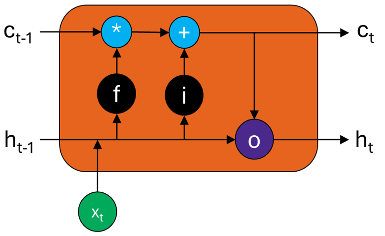
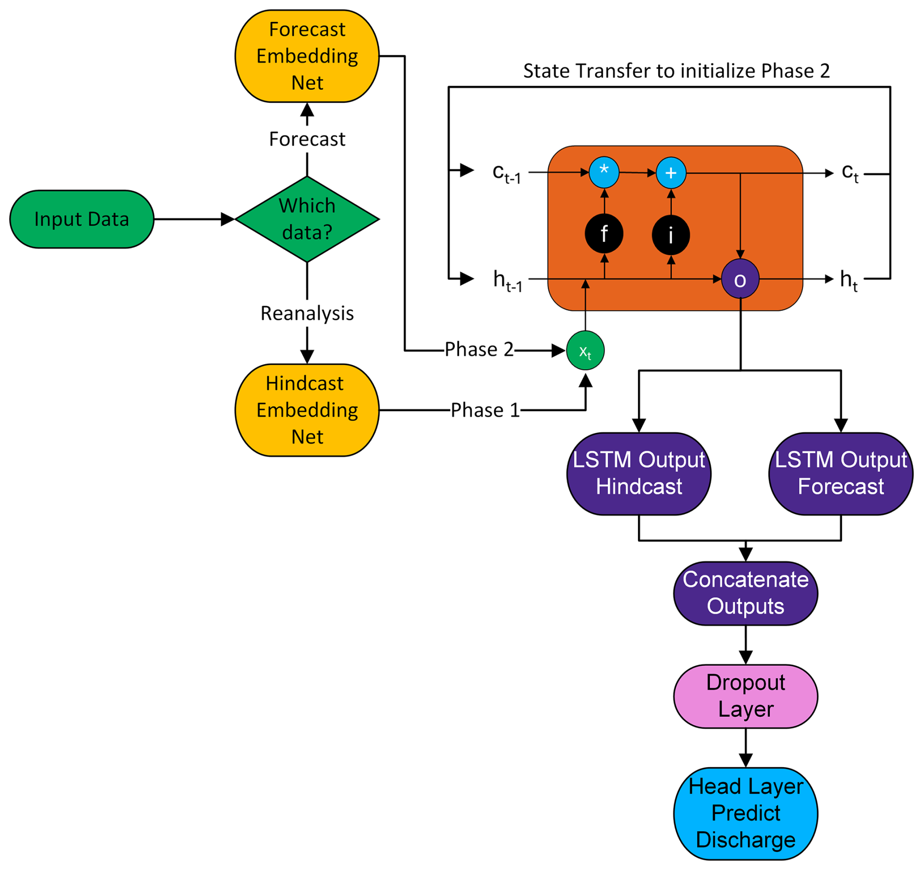
Table F1 Summary statistics of Nash-Sutcliffe Efficiency (NSE) values across all 451 basins for each experimental configuration, sorted by median NSE in ascending order. Statistics include the median, mean, standard deviation, minimum, maximum, and the 10th, 25th, 75th, and 90th percentiles. The large differences between mean and median NSE for several configurations, as well as the strongly negative minimum values, reflect the presence of extreme negative outliers in a small number of basins, which disproportionately influence the mean and standard deviation.

Appendix G: Computational Resources

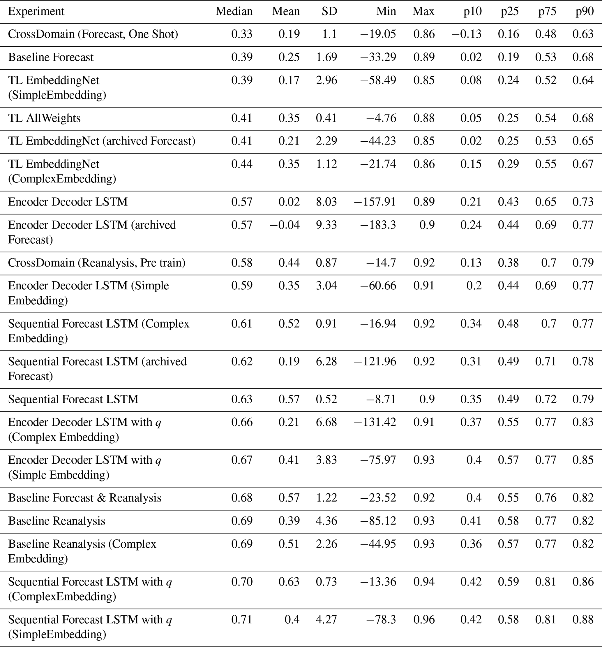
All conducted experiments were trained on a NVIDIA RTX4090 graphics processing unit, with wall times varying between several minutes to approximately 1 h for one model run, depending on the size of the input vector in the model and the model architecture itself. Although it is common practice in hyperparameter optimisation to run the same settings three times with different seedings, we have only run the tuning with one seed at a time due to computational constraints.