High resolution modelling of temporal and spatial dynamics in soil conditions in subarctic Finland using HydroBlocks model

The changing Arctic climate alters the dynamics of melting and freezing in the ground. A methodology has been developed to assess small magnitude, ice-induced earthquakes, called frost quakes, by estimating thermal stresses in the soil in Oulu, Finland. Information on temporally and spatially varying soil properties, such as soil temperature and soil ice content, is required to calculate thermal stress. Developing this methodology further on a larger scale, over the whole country, is challenging due to a lack of in-situ measurements of those parameters with high spatial and temporal coverage. However, they can be simulated using land surface models, one of which is HydroBlocks. Previously, HydroBlocks has been applied in the contiguous United States. The goal of this paper was to configure the model in subarctic and arctic Finland. However, another challenge with large scale LSMs is that they often use coarse global soil datasets, and their simplified soil presentations can introduce errors in the modelling results. For that reason, using local soil data helps to achieve a more accurate representation of soil and improves the model performance. Hence, in this paper, the HydroBlocks model was run first by using coarser SoilGrids soil data and second, by using local soil data provided by the Geological Survey of Finland (GTK). HydroBlocks' ability to produce accurate snow accumulation and melt approximations, as well as estimate soil temperature and soil water content at different depths in Finland, has not been evaluated before. The snow model (snow water equivalent) and the modeled soil temperatures and soil water contents were compared with observational data to evaluate the model performance. For six observational snow water equivalent stations, with GTK's soil data the average RMSE and KGE were 29 mm and 0.34, respectively. The worst KGE was −0.30, and the best was 0.90. For the three observational soil stations, the soil temperature had an average RMSE and KGE of 1.3 °C and 0.7, respectively. The worst KGE was 0.22, and the best was 0.86. For the soil water content, using local soil data provided by the GTK significantly improved the modelling. The average RMSE and KGE were first, 0.15 vol/vol and −3.5, and after calibration, they were reduced to 0.03 vol/vol and increased to 0.09, respectively. For the calibrated model, the worst KGE was −0.8, and the best was 0.49. The modelling results emphasize the importance of calibrating the model with local soil hydraulic parameters. The modeling results indicate that outputs from HydroBlocks can generally predict soil conditions in Finland. In addition, modelled soil ice content in Talvikangas was observed. Furthermore, the obtained soil temperature and soil ice content show potential to be used to calculate thermal stresses in soils and identify frost quake-prone areas regionally across Finland over recent decades, ultimately estimating the risk caused by frost quakes.

1 Introduction

The Arctic climate is rapidly changing (IPCC, 2023), which may have unexpected impacts on the mechanical stability of the uppermost soil layers under varying weather conditions. In particular, to processes associated with seasonal freezing and thawing. As a result, Arctic urban environments and their infrastructure (e.g., roads) are facing an increasing risk of damage (Battaglia and Changnon, 2016; Okkonen et al., 2020; Afonin et al., 2024) due to the growing frequency of ice-induced small magnitude earthquakes, frost quakes, that have been detected in these regions (Battaglia and Changnon, 2016; Leung et al., 2017). One way to approach this stability issue was presented in previous research (Okkonen et al., 2020), where a method for calculating the thermal stress in soil under different weather conditions was demonstrated. In the study, thermal stresses were estimated in sandy soil in Talvikangas, Oulu, Finland, where frost quakes had been observed on 6 January 2016 (Okkonen et al., 2020). Thermal stress σ_xx in the soil at depth z at time t can be obtained from the spatiotemporal temperature distribution (Timoshenko and Goodier, 1951), by the following equation:

$$\begin{array}{}\text{(1)}& \begin{array}{rl}{\mathit{\sigma }}_{xx}(z,t)=& -BT(z,t)+{\displaystyle \frac{B}{d}}\underset{\mathrm{0}}{\overset{d}{\int }}T(z,t)\mathrm{d}z\\ & +{\displaystyle \frac{\mathrm{12}\left(z-\frac{\mathrm{1}}{\mathrm{2}}d\right)}{d^{\mathrm{3}}}}B\underset{\mathrm{0}}{\overset{d}{\int }}T(z,t)\left(z-{\displaystyle \frac{\mathrm{1}}{\mathrm{2}}}d\right)\mathrm{d}z\end{array}\end{array}$$

Where σ_xx(z,t) is thermal stress (Pa), $B=\frac{E\mathit{\alpha }}{\mathrm{1}-\mathit{\nu }}$ is bulk modulus (Pa), E is Young's modulus (Pa), ν is Poisson's ratio (–), α is coefficient of linear expansion (°C⁻¹), T(z,t) is the soil temperature as a function of depth z, and time t (°C), and d is the thickness of frozen soil layer (m). By developing this approach to a country scale would help identify areas where accumulated thermal stress may be released in the form of frost quakes to help prepare protective procedures to safeguard crucial infrastructure. From Eq. (1), it can be seen that, in addition to soil elastic parameters, data on soil temperature and frost depth are required in the calculation of thermal stress, but in situ measurements of these parameters, with high spatial coverage, are rarely available (Kouki and Colliander, 2025).

However, regional and global land surface data exist that can be used in hydrological and land surface models (Fisher and Koven, 2020) to estimate these variables. In Finland, for hydrological forecasting and research, the Finnish Environment Institute (SYKE) has developed a conceptual WSFS (Watershed Simulation and Forecasting System) hydrological model, and further WSFS-P, a more process-based model, with a two-layer representation of soil in a 1 km² grid, which is used to model catchments and especially changes in lakes and rivers across Finland (Vehviläinen and Huttunen, 2001; Menberu et al., 2024). In addition, they also apply the Soil and Water Assesment Tool (SWAT) model (Piniewski et al., 2019) for watershed and catchment size investigations. For climate change scenarios and forest-related research, SYKE and the Finnish Meteorological Institute (FMI) have been applying the Max Planck Institute Earth System Models (MPI-ESM) land surface component JSBACH (Thum et al., 2011). In other watershed-scale studies, for example, on peatlands, the HydroGeoSphere (HGS) model (Autio et al., 2023) has been used.

Considering frost quake research, we would benefit from a model that could be used to obtain soil temperature (Soil T), and an estimate of frost depth based on soil ice content (SIC) at different depths with high spatial and temporal resolution in a country scale. One solution is to use land surface models (LSMs), such as HydroBlocks (Chaney et al., 2016, 2021). In comparison to some other hydrological models, HydroBlocks is a computationally efficient hyper-resolution model that enables country-scale simulations with a 90 m spatial resolution, basing its calculations on physical processes modelling multiple different surface and subsurface processes at different depths. Previously, HydroBlocks has been applied over the contiguous United States to estimate e.g. soil moisture, soil temperature, surface and subsurface runoffs, and to simulate groundwater dynamics (Chaney et al., 2016, 2021; Vergopolan et al., 2020, 2021; Guyumus et al., 2026).

However, for global simulations, large-scale hydrological land surface models, such as Noah-MP (Niu et al., 2011), which is also applied in HydroBlocks, and CLM (Oleson et al., 2013) among others, often apply global soil datasets, such as GLDAS dataset by NASA (Rodell et al., 2004), having a ≈ 25 km resolution, FAO soil database by the Food and Agriculture Organization of the United Nations, which has 1 km resolution (FAO, 2023), or SoilGrids, which has 250 m resolution (Poggio et al., 2021). The resolution of these soil models is coarse, and hence they tend to smooth out small-scale features and heterogeneities (Fisher and Koven, 2020; Li et al., 2024; Zhang et al., 2023). The uncertainty in large-scale soil models (Poggio et al., 2021) inherently lead to errors in calculations related to the carbon cycle (Koven et al., 2013) and estimations of hydrological variables (Fisher and Koven, 2020; Zhang et al., 2023). Consequently, using a more accurate representation of soil is essential and the emphasis on using high-resolution soil data has previously been demonstrated in other regions such as USA (Singh et al., 2015), South America (Maertens et al., 2021) and China (Ji et al., 2023). One way is to use local soil data, and in Finland, the Geological Survey of Finland (GTK) has mapped the Finnish soil and provides available datasets.

In this paper, HydroBlocks is applied over Finland, located in boreal, Subarctic, and Arctic regions between latitudes of 59 and 71° and longitudes of 20 and 32°, first using SoilGrids soil data and second, using soil data provided by the GTK, demonstrating how the simulations can be improved by using local soil data. Before using the outputs from HydroBlocks in other applications, it is essential that the hydrological simulations are as reliable as possible. In-situ soil water equivalent (SWE) data from six stations across Finland are used to validate HydroBlocks SWE simulations. Additionally, in-situ liquid soil water content (SWC) and soil T data from three locations in Finland are used to validate HydroBlocks simulations of the same parameters. Furthermore, from the model it is possible to obtain the SIC at different depths in the soil. The structure of the paper is as follows:

1. The description of HydroBlocks, study area, model setup, and parameterizations.

2. Input data used in the model: meteorology and land surface datasets, with main differences between SoilGrids soil data and GTKs soil data.

3. Model calibration and observational data: Snow water equivalent (SWE) from six snow stations, and soil station data of soil temperature (Soil T) and soil water content (SWC), from three soil stations.

4. Additionally, modelled timeseries of SIC in Talvikangas.

5. Discussion and conclusions.

This study utilizes a field-scale-resolving land surface model for the first time to estimate variable fields relevant to approximating thermal stresses – soil T and SIC (via SWC). Ultimately, we anticipate that this will lead to a more accurate and realistic understanding of frost quakes in Arctic regions under the changing climate. This study describes the HydroBlocks modeling workflow and the evaluation of the simulations against in-situ measurements.

2 Data & Methods

2.1 HydroBlocks

HydroBlocks model is configured for Finland, located in Northern Europe, between latitudes of 59 and 71° and longitudes of 20 and 32°, (Fig. 1). HydroBlocks (Chaney et al., 2016, 2021), a land surface model, uses a clustering algorithm to group grid cells of assumed similar hydrological response into Hydrologic Response Units (HRUs) based on datasets of high spatial resolution, such as elevation, soil properties, and land use, that describe the surface spatial heterogeneity. The HRUs are defined by the Hierarchical Multivariate Clustering (HMC) algorithm (Chaney et al., 2021). This approach begins by first splitting a large model domain, for this study, Finland (Fig. 2a) into smaller subdomains, which are shaped as polygons following the natural drainage divide. The basis for delineating the subdomains is a Digital Elevation Model (DEM) used to define the river network and watersheds. The boundaries of the subdomains are adjusted in a way that no watershed is split between polygons, and they only belong to the polygon where they fall the most This becomes evident in Fig. 2b, showing the clusters of watersheds, where the watersheds defined by the model extend beyond the boundary (red square) of the subdomain.

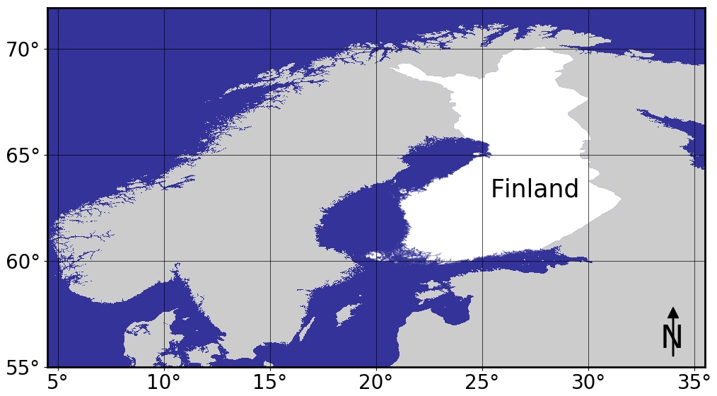
Figure 1 The location of Finland in Northern Europe. Country extents extracted from the MERIT DEM (Yamazaki et al., 2017) and from the National Land Survey of Finland land cover dataset (MML, 2024), downloaded July 2024. (The coordinate system is WGS84 & units are latitude and longitude.)

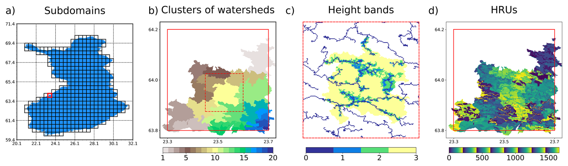
Figure 2 (a) The model domain is divided into 435 subdomains. (b) Close up to the highlighted subdomain framed with red color: clusters of watersheds obtained with k = 20. (c) The height bands in one cluster of watersheds, framed with a dashed red line, in the previously highlighted subdomain. (d) HRUs in the same subdomain after clustering intraband clusters with p = 20.

Second, the watersheds within each subdomain are grouped into clusters of watersheds by using K-means clustering based on watershed-aggregated covariates (Fig. 2b). In this study, the selected covariates include dem, latitude and longitude. In addition, the empirical cumulative distribution functions (CDF) of HAND values (height above nearest drainage) are calculated for each watershed, which is then set to an average of the HAND empirical CDFs of the watersheds in a cluster of watersheds. This ensures the similarity of the watersheds that are clustered together. Thirdly, from the HAND values, each cluster of watersheds is discretized into height bands, i.e., into a channel and a floodplain component (Fig. 2c). The area of each height band increases as they move further away from the channel, and the next height band has n times the area coverage of the previous height band. The last step in defining the HRUs is to cluster pixels within each height band into intra-band clusters based on pixel-based covariates, including latitude, longitude, land cover, and clay content, to account for small-scale heterogeneity (Fig. 2d).

Pixels that form the HRUs, do not have to be spatially connected. Still, each HRU is presumed to be homogeneous by taking the average of the meteorological and land data in the pixels that are clustered into the same HRU. Considering the number of HRUs that each subdomain has, at one end of the scope, in theory, a single HRU would be used to describe the whole subdomain. Undoubtedly, with one HRU, it is challenging to capture the real heterogeneity of an extensive land surface area. At the other end of the spectrum, in a fully distributed simulation, each pixel would be its own HRU. However, as a more detailed division is made, more computational power is required. Therefore, a balance between the number of HRUs and computational power is needed to approximate the fully distributed model. The number of HRUs will affect the simulation results. It has been demonstrated that using 1000 HRUs over 610 km² (Chaney et al., 2016) is sufficient to represent the fully distributed solution while maintaining the model's computational efficiency. In more recent work, with the more evolved HydroBlocks (Chaney et al., 2021), it was concluded that a reduced number, 300–350 HRUs, is appropriate to model a 0.25° × 0.25 ° model domain to approximate the fully distributed solution. However, it is worth mentioning that these are still location- and application-specific scenarios.

In total, the whole model domain, Finland, (12° × 12°) is divided into 36 sections (2° × 2°), and each of them has a maximum of 25 subdomains of 0.4°. In total, 435 subdomains were used for the modelling. HydroBlocks' HMC generates 683 689 HRUs using parameters k=20, n=2, p=20. As described in Sect. 2.1, the model defines the HRUs by delineating the river network and watersheds in all land areas and further clusters pixels hierarchically. This method makes small islands problematic. Hence, Åland, the archipelago of Turku, and the islands along the southern and Western shorelines are excluded from the model.

HydroBlocks uses the vertical column model Noah-MP (Niu et al., 2011) within the HRU framework to represent surface and subsurface processes at a field scale. Each time step, the land surface scheme updates the hydrological states for each HRU; these HRUs interact laterally through subsurface flow at every level of the soil column by computing Darcy's flux and adding it as a divergence term to the vertical solution of Richard's equation in Noah-MP to update the next time step (Chaney et al., 2021). The selected depth of the soil column is 2 m, and the total number of soil layers is 9, located at 10, 20, 30, 40, 50, 60, 90, 120, and 200 cm depth. HydroBlocks is run for years 2000–2023. The model updates every 20 minutes, but the results are reported on an hourly basis. To evaluate possible trends in the data, the model was run for the same 50-years as a spin-up period. From this procedure, it was concluded that the required spin-up period for the model is between 3 and 5 years. Consequently, in the final simulation, the year 2000 is run 5 times for the model to reach numerical stability, making the physics and dynamics more consistent.

2.2 Noah-MP

Noah-MP (Niu et al., 2011) is a more evolved version of the original Noah LSM, with the ability to utilize multiple parametrization. Specifically, Noah-MP offers options for various physical and hydrological processes, allowing the user to choose schemes based on their modeling purposes. Noah-MP simulates various subsurface processes, including recharge, changes in the water table, and base flow. At each time step, the model calculates soil moisture and vertical water flow in unsaturated soils across different soil layers using the one-dimensional Richards equation.

In Noah-MP, the soil column is composed of a user-defined number of layers, and snow cover is modeled with a maximum of three layers, depending on the time-specific snow depth. The snow depth (density) is estimated by taking into consideration how new snow, melting, and refreezing affect the snowpack. The model accounts for the compaction of snow caused by layers above and within a single layer, as well as thermal and melt metamorphism. Considering the ground surface, Noah-MP regards the vegetation canopy as an individual layer, which enables the computation of the surface and canopy temperatures separately. In comparison to bare ground, forested ground intercepts rain and snowfall, and absorbs sunlight differently, consequently affecting the resultant amount of snow on the ground, runoff production, and soil temperature. There is an option for dividing precipitation into rainfall and snowfall. For our purposes, the simplest criterion is chosen, in which all the precipitation comes down as snowfall when the surface air temperature is smaller than the freezing point of water. For snow-soil temperature (snow layer 1), the option with temperature flux between the snow and soil was chosen.

For runoff and groundwater, there are options for a simple groundwater scheme (Niu et al., 2007) and a TOPMODEL-based runoff scheme with an equilibrium water table (Niu et al., 2005). Surface and subsurface runoffs are defined as exponential functions that depend on the depth of the water table. With the first option, the saturated hydraulic conductivity decays exponentially towards the bottom of the soil column, and the model places an aquifer below the soil column. With the second option, the equilibrium water table extends the soil column and performs a water distribution based on the water deficit. The first option is chosen because it reduces the water in the soil column. In addition, there is an option to restrict a zero heat flux from the very bottom of the soil column as a lower boundary condition or, alternatively, use a user-defined value of soil temperature at 8 m depth. The latter is chosen.

Considering more details on frozen soil properties, there is residual water near the soil particles that remains in liquid form even when the soil freezes. The upper limit for this super-cooled liquid water is a function of soil temperature and soil texture class properties, and it defines the maximum amount of liquid water remaining in the frozen soil layer. Koren's iteration (Koren et al., 1999) is chosen, which implements the freezing-point depression equation with an extra term that takes into account also the water around ice particles. Additionally, there are options for the “frozen soil permeability.” The chosen option assumes that soil ice reduces the total permeability (Koren et al., 1999). Considering soil ice content (SIC), the model outputs the liquid soil water content (SWC) and also the total soil moisture content (SMC), which consists of both liquid and frozen water. Consequently, SIC can be obtained from SMC and SWC as a percentage of frozen water to the whole moisture content.

2.3 Study area and input data

As input, HydroBlocks requires various types of land surface data, including meteorology, surface elevation, soil thickness, land use, and soil types. The meteorological data is obtained from the Era5 LAND dataset, which is a global climate model (Muñoz-Sabater, 2019). Era5 has been created by combining climate modeling and observational meteorological data via atmospheric forcing. The dataset ranges from 1950 to the present, with a spatial resolution of 9 km and a temporal resolution of 1 h. The meteorological data used include air temperature, precipitation, air pressure, the Eastward and Northward components of wind, and solar radiation (both short-wave and long-wave).

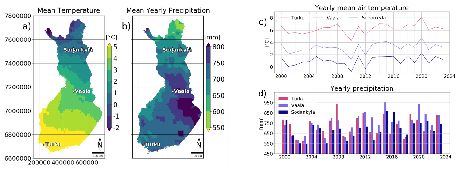
Figure 3 (a) Mean temperature [°C]. (b) Mean yearly precipitation [mm], between 2000–2023, and three locations from which there are time series of the corresponding variables. (c) Mean temperature [°C] and (d) mean yearly precipitation sum [mm], between 2000–2023 in Sodankylä, Vaala, and Turku. Original meteorological data from Muñoz-Sabater (2019). (The coordinate system is ETRS-TM35FIN & units are in meters.)

In Fig. 3a and b, the mean temperature and yearly precipitation sum between 2000–2023 is calculated from the Era5 LAND dataset. These maps are similar to yearly statistics from 1991 to 2020 calculated by The Finnish Meteorological Institute, FMI (FMI, 2024a). However, based on visual inspection, the amount of precipitation is higher in Era5 LAND. Although, the years are not the same in both datasets. Further, Fig. 3c and d show time series of air temperature and precipitation for three locations, Sodankylä, Vaala, and Turku created from the ERA5 LAND dataset. It is worth mentioning that in Finland, the yearly temperatures are generally warmer in southern Finland than in northern Finland. Whereas Eastern Finland, located inland, experiences most of the precipitation, and the northernmost regions experience the least. Furthermore, these factors result in varying winter weather conditions across Finland.

Figure 4 (a) Raster map of generalized land cover. Data extracted from SYKE (2018). (b) Terrain elevation [m], data from Yamazaki et al. (2017). (c) Soil thickness [m], data from GTK (2023).

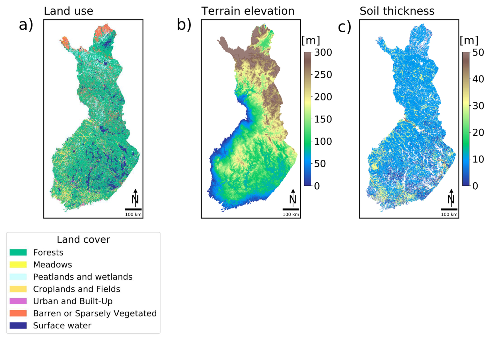
A raster map, with a resolution of 20 m of the land use characteristics (Fig. 4a), is created from the CORINE Land Cover 2018 dataset obtained from the Finnish Environment Institute, SYKE (SYKE, 2018). Elevation data is provided by the MERIT DEM (Yamazaki et al., 2017), which is a global dataset of terrain elevation with a 90 m spatial resolution (Fig. 4b). The soil thickness i.e. Superficial deposit thickness (Fig. 4c), was obtained from The Geological Survey of Finland (GTK, 2023). The dataset has a resolution of 250 m, but it has some missing values in the data, especially in Northern Finland, which are interpolated for the model.

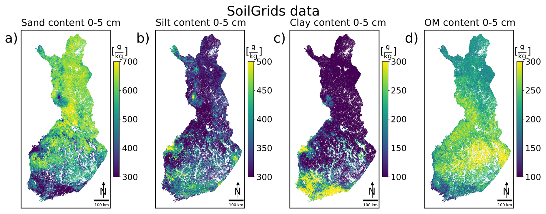
Figure 5 Soilgrids data [g kg ⁻¹] at 0–5 cm depth (a) sand content, (b) silt content, (c) clay content, (d) organic carbon content. Data from Poggio et al. (2021), downloaded July 2024.

Soil texture classes are determined with the USDA classification based on the data from the SoilGrids database (Poggio et al., 2021), a global soil model created by combining machine learning, modeling, observations, and environmental covariates. The International Soil Reference and Information Centre has developed the database. The dataset provides the contents of sand, silt, clay, and organic carbon at six different depths: 0–5, 5–15, 15–30, 30–60, 60–100, and 100–200 cm. Figure 5 shows SoilGrids data from the topsoil. This dataset has a resolution of 250 m. SoilGrids' ability to give information not only spatially over Finland but also vertically makes it suitable for modeling purposes in this study. The derived soil texture classes (Fig. 6a) divided the Finnish soil into three main categories: sandy loam, loam, and clay loam. “Other” comprehends all the other soil texture classes.

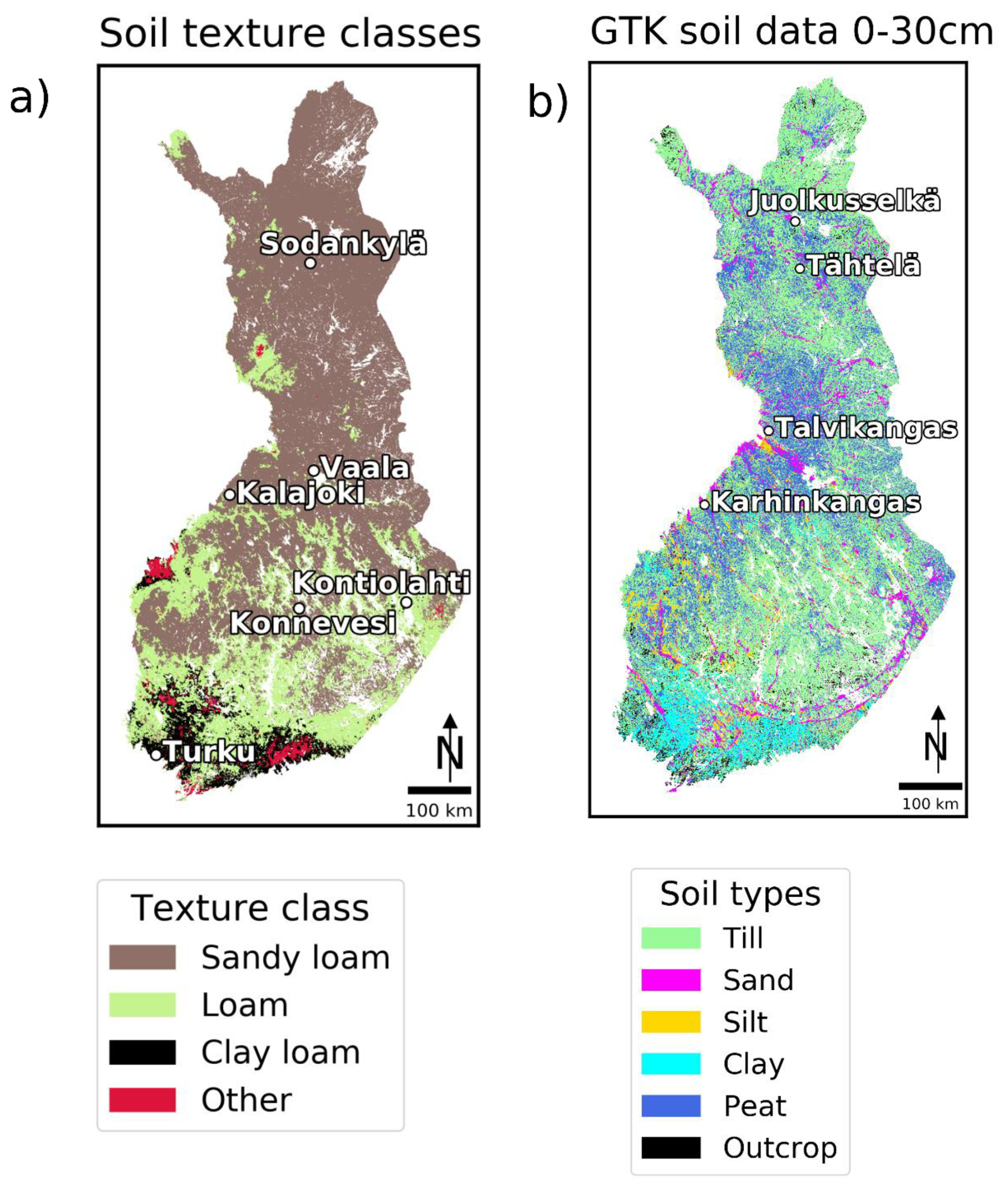
Figure 6 (a) Soil texture classes created based on the USDA classification and SoilGrids data with the locations of the six snow stations. (b) Main soil types in Finland, at 0–30 cm depth, defined for HydroBlocks from the GTK's surficial deposits 1 : 200 000, with the locations of the three soil stations: Karhinkangas, Tähtelä, and Juolkusselkä, and the location of Talvikangas. Data modified from the (GTK, 2023), downloaded August 2025.

However, in reality, Finnish soil cover is much more variable, which is evident from the superficial deposits defined by the Geological Survey of Finland (GTK, 2023). Finnish soil is a product of the latest glacial period, and the Finnish landscape is characterized by eskers, drumlins, and other glacial formations (Ympäristöministeriö, 2023; Ronkainen, 2012). The primary soil type is glacial till, which is missing from the USDA classification, comprising a diverse mixture of large and small grains of different compositions. In addition, clay-rich soils cover over 8 % of the land cover, located mostly in Southern Finland (GTK, 2023). As well as over 30 % of land is covered by peat lands, of which a bit over 15 % have peat depth over 1 m (GTK, 2023). In addition, another problem is that the organic material (OM) in the SoilGrids dataset is quite low, with the highest values around 30 %–55 % in Finland. The soil is defined as an OM texture class only if the OM content is > 75 %, which is also the definition of peat. In addition, the USDA soil texture class division and given values for the soil characteristics have been developed for USA soil (Saxton and Rawls, 2006). Therefore, the USDA texture classes and their hydrological characteristics do not align precisely with those of Finnish soil.

Hence, GTK's soil data is used as another source of soil, to improve the modelling. The superficial deposits 1 : 200 000 (Fig. 6b) was chosen because it covers the whole Finland. However, it should be noted that in reality, there can be even more variation in the soil type on a small spatial scale. GTK's 1 : 200 000 dataset describes the soil types at the top of the soil column, at 0–90 cm, and at 1 m depth. In addition, the dataset provides coarse information on the depth extent of the top peat layer, whether organic material reaches 0–30, 30–60, or over 60 cm depth. The main soil types in the dataset are mixed soil (glacial till), coarse-grained soil (sand and gravel), fine-grained soil (silt), clay, gyttja, gyttja-rich fine-grained material, organic material, bedrock, bedrock with thin soil on top, rocks, fill, and built-up. Gyttja is a lake sediment formed by partial decomposition of organic material, consisting in total of 6 %–40 % of organic material mixed with mineral soil (GTK, 2023). In this dataset gyttja category also comprehends clay and silt soils, which are gyttja rich (6 %–8 %). However, the prevalence of gyttja and gyttja-rich fine-grained soil is around 0.5 % of all pixels; hence, they were simplified into the OM category.

Further, for modelling purposes, soil layers were created for four depths, 0–30, 30–60, 60–90, and 90–200 cm. The first three layers have the top soil data from the GTK's dataset, and the fourth layer has the 1 m soil data. In addition, for the peat depth, the possible maximum depths of 30, 60, and 90 cm were taken into account when creating the soil layer files, and the bedrock with thin soil on top has a maximum of 1 m of soil cover, and it was assumed to reach 90 cm. Additionally, urban areas were generally unmapped and were generalized into the till category, with “fill” and “built-up” to prevent large gaps in these areas.

2.4 Model calibration and in-situ data

Some of the most critical aspects when simulating soil conditions in Subarctic Finland are the wintertime snow cover, snow melt, the soil types, and the hydrologic properties of those soil types. In Finland, snow accumulates and melts differently in the south, north, west, and east (FMI, 2023) due to different climate conditions. The Finnish Environment Institute (SYKE) measures SWE (Snow line measurements from SYKE, 2024) values across Finland (SYKE, 2022), generally twice a month. For model validation, data from six snow stations in the cities/municipalities of Sodankylä, Vaala, Kalajoki, Kontiolahti, Konnevesi, and Turku, were chosen because they are located at different latitudes and longitudes across Finland. Their locations are shown in Fig. 6a. Noah-MP has options for the snow melt curve parameter (MFSNO), which can be set based on the land use type. MFSNO was originally 2.5 everywhere for every land cover type. The values for the MFSNO parameter were optimized based on (He et al., 2019) for each of the land cover types. Based on visual inspection, this slightly adjusted the modeled SWE values.

In situ data on soil types from three soil stations are also available, and their locations are shown in Fig. 6b. Two of them are soil stations of the GTK located in Karhinkangas, Kokkola (Tähtikarhu and Okkonen, 2023), and in Juolkusselkä, Sodankylä (Liwata et al., 2014). In Karhinkangas, soil T and SWC were collected at 10 different depths (5, 10, 20, 30, 50, 80, 110, 140, 170, and 200 cm) between 11 September 2011 and 30 May 2015 and in Juolkusselkä at three different depths (20, 40, and 60 cm) between 3 April 2008 and 11 June 2014. In Karhinkangas, the soil type is sandy soil (Tähtikarhu and Okkonen, 2023), and in Juolkusselkä, it's sandy till (Liwata et al., 2014).

Table 1 Soil types at the locations of the soil stations from different sources.

Soil types at the locations of the three soil stations from in situ measurements: ^a Okkonen et al. (2020) and ^b Liwata et al. (2014), from the Superficial deposits database of ^c Geological Survey of Finland GTK (2023), and in the HydroBlocks model based on the USDA classification from SoilGrids data.

In addition, in the ADAPTINFA project, a soil station in Tähtelä, Sodankylä, in northern Finland was installed on 20 October 2022. Soil T and SWC have since been collected at five different depths (10, 20, 30, 50, and 80 cm). Additionally, soil samples were taken from the soil pit when the soil station was installed in the ground in Tähtelä, and based on the particle size distributions determined with sieve analysis, the soil type in Tähtelä is medium-grained sand. In Table 1, there is an overview of the differences between soil types/soil texture classes at the locations of the three soil stations from different sources: from in-situ measurements, from the GTK, and based on the USDA classification. It can be noted GTK's soil data aligns closely with in-situ measurements. However, USDA classification from SoilGrids soil data defines sandy loam at all three soil station locations.

Table 2 Hydraulic parameters of Finnish soil collected from different sources, for HydroBlocks M2.

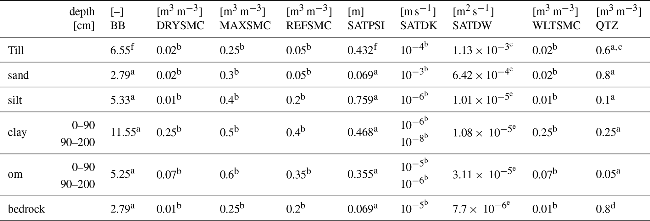
Data from ^a Niu et al. (2011), ^b Kolhinen et al. (2026), Jakkila et al. (2014), ^c Middleton et al. (2011), ^d Haldorsen (1983). ^e From equations profided in Kishne et al. (2017). ^f Average of sand, silt and clay.

Additionally, multiple parameters influence the accumulation of moisture in the soil profile. In Noah MP, there are values for the characteristics of soil texture classes, i.e., soil types (Niu et al., 2011), such as porosity, saturated soil water diffusivity, saturated soil hydraulic conductivity, quartz content, etc., which affect the SWC (and soil T). There are studies (Kishne et al., 2017; Saxton and Rawls, 2006)) on how the default Noah-MP values are defined or calculated and how measured values of the hydraulic soil parameters differ from the default Noah-MP values in the model. For the GTK's soil data the hydraulic properties table is modified (Table 2), to represent Finnish soil more accurately, based on available literature sources. It should be noted that in reality, all of these hydraulic properties have variations within a soil type, and it is impossible to have a single value to describe a soil property across the whole country. In the future, other methods, such as creating probabilistic maps of soil properties (Chaney et al., 2019), to better estimate these parameters should be sought. This study presents the results from two final models, referred to as Model 1 (M1) and Model 2 (M2). The difference is that M1 has SoilGrids data with a default table of soil hydraulic parameters (Niu et al., 2011), while M2 has soil data from the GTK and a table of soil hydraulic parameters collected from literature sources, Table 2.

3 Results

Time series of SWE, soil T, and SWC obtained from HydroBlocks (M1 & M2) were validated against observational data of the same parameters from 6 snow stations (Sodankylä, Vaala, Kalajoki, Kontiolahti, Konnevesi, and Turku) and three soil stations (Karhinkangas, Tähtelä, and Juolkusselkä). RMSE and KGE were used to evaluate model performance. The SWE values were first validated, because snow on the ground directly impacts the subsurface conditions. The modelling shows, that soil T can be modelled reasonably well. SWC predictions are improved by using local soil data, which subsequently highlights the importance of using adequate soil data and soil hydrologic parameters. A better estimation of SWC, makes also SIC more reliable.

3.1 Snow water equivalent

Snow cover and snowmelt affect soil temperature and the distribution of water and ice; therefore, simulated SWE is first validated. Figure 7 shows the time series at the SWE stations from M1 and M2, and their corresponding RMSE and KGE values are presented in Table 3. Figure 7 shows the SWE time series from different snow stations from M1 and M2, and their corresponding RMSE and KGE values are presented in Table 3. In addition, Fig. 8 shows shorter time series from SWE station with the best and worse KGE

Figure 7 Results from HydroBlocks simulations: M1 (purple line) and M2 (black line) with observed (colored dots) of SWE [mm] in Finland 2000–2023 at the six observational snow stations. Snow line measurements from SYKE, The Finnish Environment Institute (SYKE, 2024).

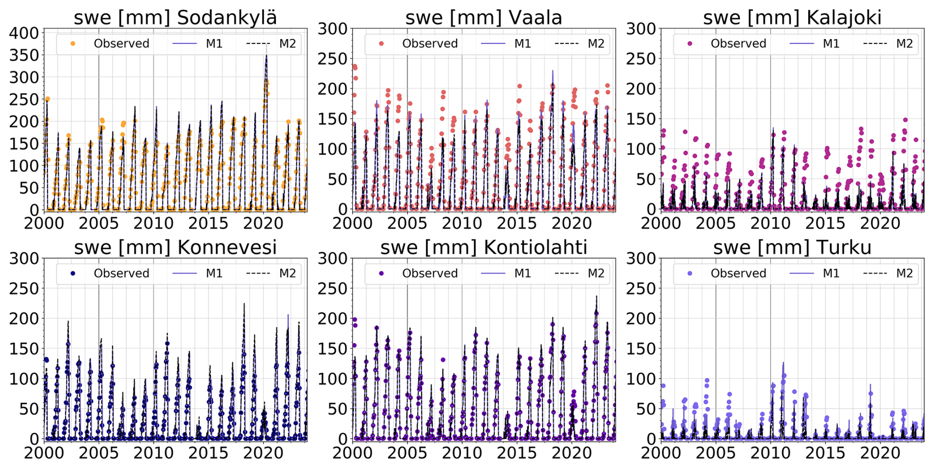
Table 3 Model statistics: RMSE and KGE values for the six snow stations in M1 & M2.

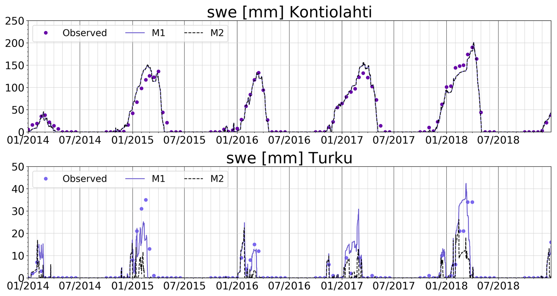
Figure 8 Results from HydroBlocks simulations: M1 (purple line) and M2 (black line) with observed (colored dots) of SWE [mm] in Finland 2014–2018 at two observational snow stations; Kontiolahti (the best KGE), and Turku (the worst KGE). Snow line measurements from SYKE, The Finnish Environment Institute (SYKE, 2024).

When comparing the timeseries of modeled SWE responses to observations of SWE, it can be observed that the model provides reasonable values. Notably, in the winter months, there is a thicker snowpack in Northern Finland (Sodankylä) compared to Southern Finland (Turku). When comparing the RMSE values between M1 and M2, they do not really vary, except in Vaala and Turku. Considering the KGE values between the snow stations, the difference between the two settings is marginal for each of the analyzed stations, except for Turku, where most likely the change in soil type and hence, the soil quartz content, which affects the soil thermal conductivity, has an effect on the accumulation of snow. In Sodankylä, Vaala, Kontiolahti and Konnevesi satisfactory values are obtained. However, in Kalajoki, the values are unsatisfactory, and in Turku, the M2 does not behave very well.

3.2 Soil temperature, soil water content, and soil ice content

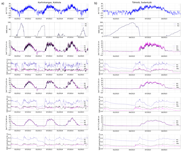
Furthermore, the simulated soil T and SWC are compared with observational data obtained from the three soil stations. The time series of the soil T and SWC for both HydroBlocks experiments corresponding to the locations of the three soil stations are evaluated against observational data from the same depths. Figure 9a shows soil T [°C] and SWC [vol/vol], respectively, at depths of 5, 20, and 50 cm at the Karhinkangas, Kokkola soil station, Fig. 9b at depths of 10, 30, and 50 cm at the Tähtelä, Sodankylä soil station and Fig. 10 at depths of 20, 40, and 60 cm at the Juolkusselkä, Sodankylä soil station. In addition, the air T [°C] and modeled SWE responses [mm] are also shown in each graph. In addition, Tables 4, 5, and 6, show the corresponding RMSE and KGE values for the three soil stations from both experiments.

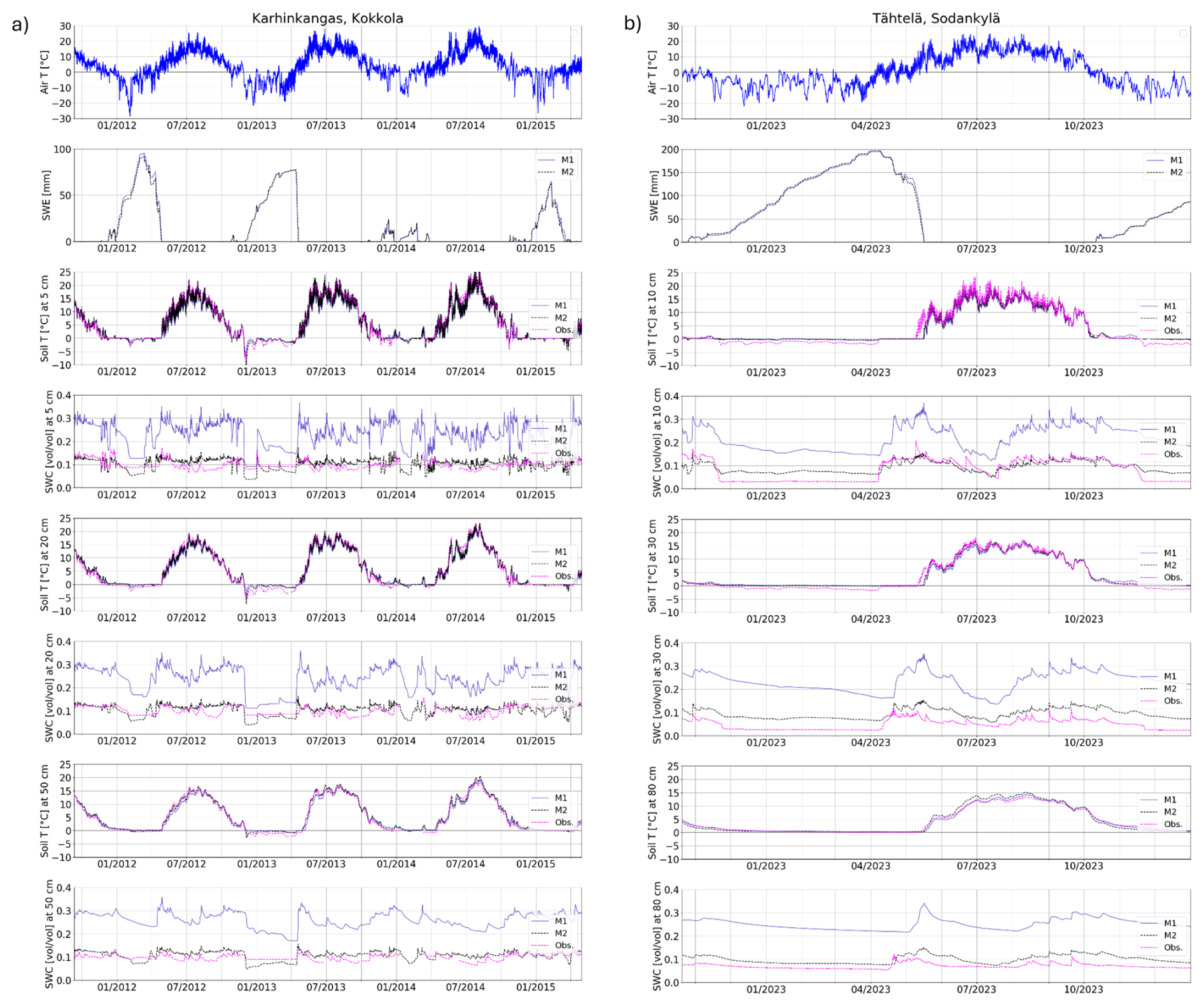
Figure 9 Results from HydroBlocks simulations M1 (purple line), M2 (black line) with observed (pink line) soil T [°C] (on the left) and SWC [vol/vol] (on the right) (a) in Karhinkangas, Kokkola at 3 different depths 5, 20, and 50 cm on 11 September 2011–30 April 2015, (b) in Tähtelä, Sodankylä at 3 different depths 10, 30, and 80 cm on 20 October 2022–31 December 2023. Additionally, there are input air T [°C] and modeled SWEs [mm] over the same period in both graphs. Karhinkangas obsevational data from Tähtikarhu and Okkonen (2023).

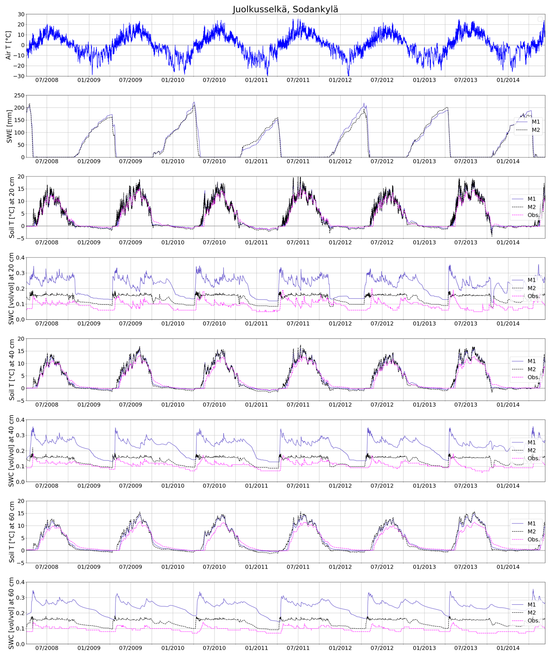
Figure 10 Results from HydroBlocks simulations M1 (purple line), M2 (black line) with observed (pink line) soil T [°C] (on the left) and SWC [vol/vol] (on the right) in Juolkusselkä, Sodankylä at 3 different depths 20, 40, and 60 cm on 23 April 2008–11 June 2014. Additionally, there are input air T [°C] and modeled SWEs [mm] over the same period in both graphs. Observational data from Liwata et al. (2014).

Table 4 Model statistics: Calculated RMSE and KGE values at the Karhinkangas, Kokkola soil station, in M1, and M2 for soil T and SWC at 5, 20, and 50 cm depth.

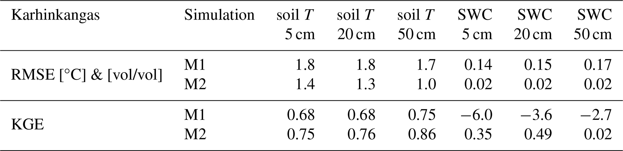
Table 5 Model statistics: Calculated RMSE and KGE values for the Tähtelä, Sodankylä soil station in M1 and M2 for soil T and SWC at 10, 30, and 80 cm.

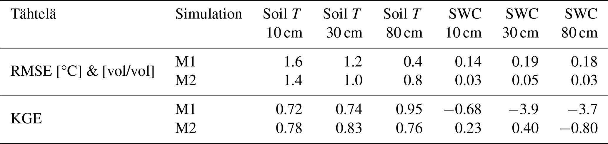
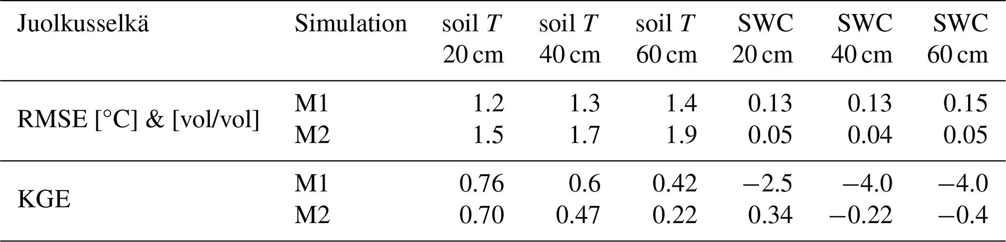
Table 6 Model statistics: RMSE and KGE values for the Juolkusselkä, Sodankylä soil station in M1 and M2 for soil T and SWC at 20, 40, and 60 cm depth.

In Karhinkangas, the modeled and observed soil T follow each other relatively well (Fig. 9a), and the responses become smoother deeper in the soil. Based on the statistical analysis, the RMSE values of soil T between M1 and M2 decrease at maximum by 0.7 °C with a mean RMSE over the three depths of 1.8 °C for M1 and 1.2 °C for M2, and the mean KGE of 0.7 for M1 and 0.8 for M2, which indicates outstanding model performances for M2. Furthermore, when observing the SWC, it can be noted that the statistical analysis indicates that for the M1, the RMSE and KGE values for SWC are not good. Over the three depths, the mean of RMSE is 0.15 vol/vol, and the mean of KGE is −4.1. However, by using GTK's soil data in M2, the modeled SWC reduces closer to the observational values. The statistics are improved in M2; the mean of RMSE is reduced to 0.02 vol/vol, and the mean of KGE is increased to 0.29.

The observations at the Tähtelä soil station (Fig. 9) start from 20 October 2022, which makes the time series shorter than the other. The statistical analysis indicates that the RMSE values of soil T do not change much between the M1 & M2, only by 0.4 °C with an overall mean of RMSE 1.1 °C for M1 and M2. The mean of KGE is 0.8 for M1 and M2, which indicates an outstanding model performance. Considering soil water content, for M1, the mean RMSE is 0.17 vol/vol, and KGE was −2.8, and for M2, the mean RMSE is 0.04 vol/vol and KGE is −0.06. In Juolkusselkä, in the summertime, the modelled soil Ts are generally a little bit higher than the observations indicate. The change in RMSE values is at a maximum of only 0.5 °C between M1 and M2, with a mean RMSE of 1.3 °C for M1 and 1.7 °C for M2, with KGE of 0.59 for M1 and 0.46 for M2. Considering SWC, for M1, the mean RMSE is 0.14 vol/vol , and KGE is −3.5, and for M2, the mean RMSE was 0.05 vol/vol and KGE was 0.05.

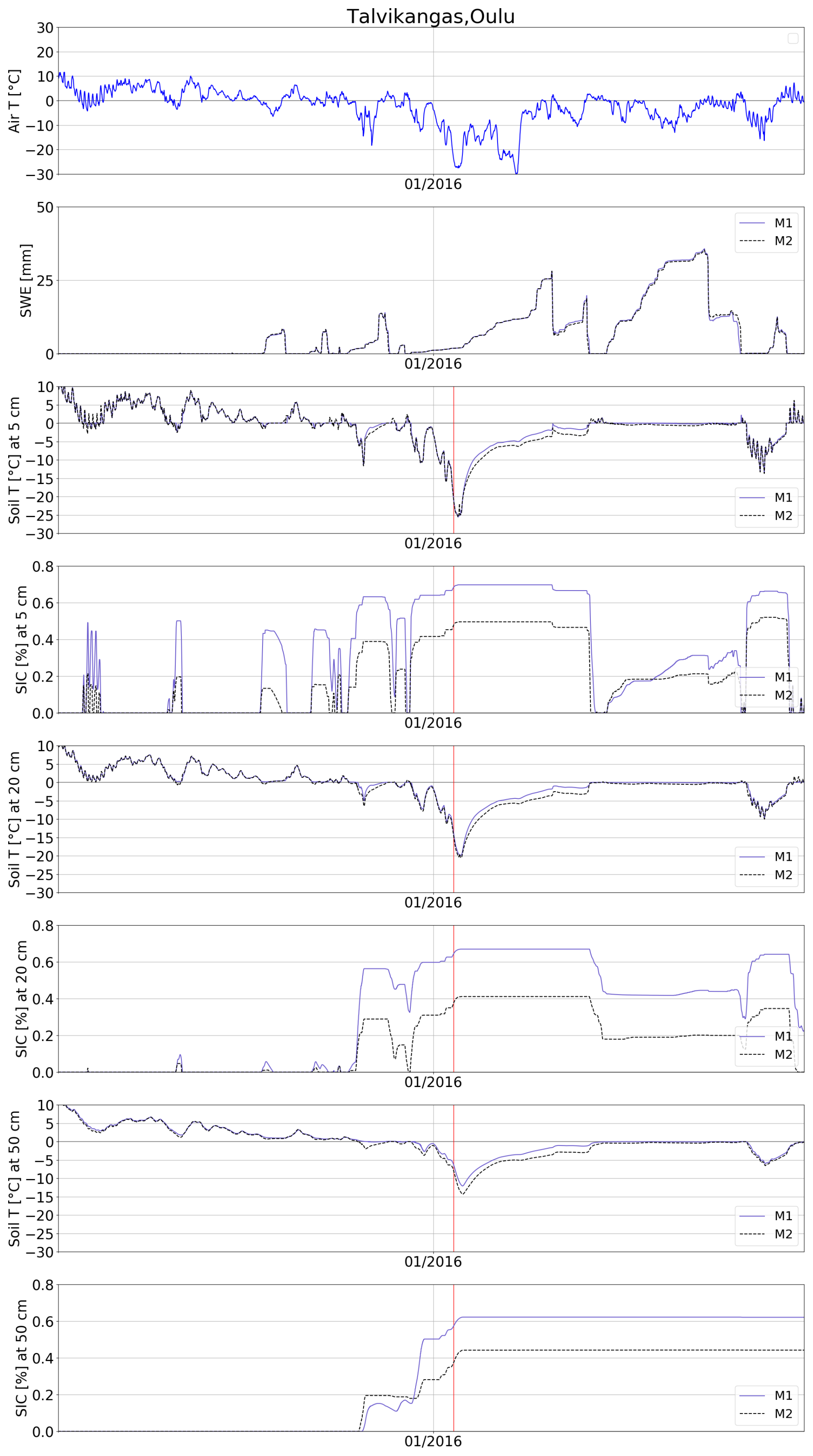
Figure 11 Results from HydroBlocks simulations M1 (purple line) and M2 (black line) of soil T [°C] and SIC [%] in Talvikangas, Oulu at 3 different depths 5, 20, and 50 cm between 1 November 2015 and 1 April 2016. Additionally, there are also the air T [°C] and modeled SWEs [mm] over the same period in both graphs, and 6 January 2016 is marked with a red line.

Additionally, a time series of modelled SIC for winter 2015–2016 in Talvikangas, Oulu, is observed (Fig. 11). It shows the air T [°C], the modeled SWEs [mm], Soil T [°C], and the modeled SIC [%] at the depths of 5, 20, and 50 cm from M1 and M2 with a red line marking 6 January, when frost quakes were observed in the area. It can be noticed that both models predict that the soil is frozen in winter. Reasonably, the topsoil has the most ice, and ice depth differs with soil T. M1 estimates that ice reaches deeper than M2.

4 Discussion and Conclusions

The modeling shows that HydroBlocks can generally predict snow and soil conditions in Finland. Over 24 years, the modeled SWEs indicate more snow in Lapland during winters and less snow in Southern Finland, which is in agreement with the observations. The model behaves well at most of the observational snow stations but less satisfactory on two of them. Considering soil T, the model performance is excellent. Moreover, the winter months (November–February) are the most critical periods for frost quake occurrences because the soil needs to be frozen. It appears that the model can simulate frozen soil conditions. Additionally, considering the actual road conditions, snow is cleared away regularly. In the model, this is not taken into account. Therefore, in reality, the temperatures may be even lower without an insulating snow cover. Although it is possible to have frost quakes even with snow on the ground.

When observing the behavior of SWC, which is related to the SIC, is that the fluctuations in the observations are also reflected in the modeled responses, which indicates that the model dynamics work. The most notable feature in each of the profiles is the stagnant lines in SWC, which indicate periods when there is ice in the soil, leaving only a residual water content. With the application of HydroBlocks on a regional scale over Finland, the biggest concern is related to the evaluation of the SWC, which is highly dependent on site characteristics and can change significantly within a small spatial window. Consequently, it should be noted that it is troublesome to use only a single value of soil hydraulic properties for each soil type in a country-scale model. Parameters controlling soil moisture need to be calibrated spatially to obtain more accurate regional modeling results.

Additionally, a comparison is performed between Era5Land and one meteorological station of the Finnish Meteorological Institute, FMI, in Tähtelä. From Fig. 12, it can be noted that the monthly mean air T between FMI and Era5land matches pretty well. However, there is much more variation in monthly precipitation sum; generally, Era5land has more precipitation than FMI. The differences in precipitation affect the snow accumulation and also the SWC. Smoother air T affects the highest and lowest of simulated soil T.

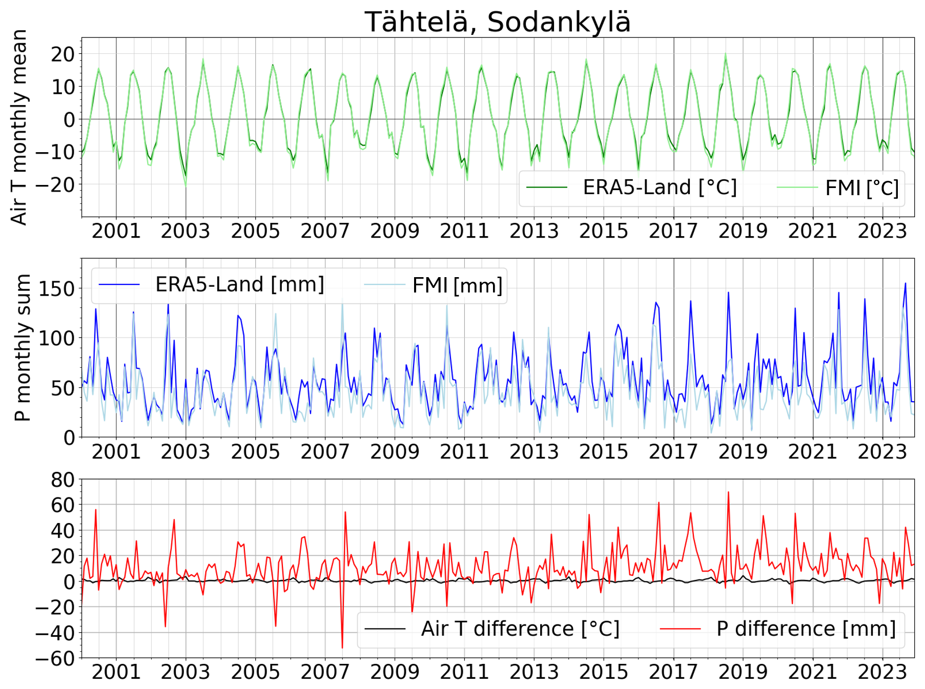
Figure 12 Comparison between monthly air T and monthly precipitation sum in Era5Land and FMI datasets. Data from Muñoz-Sabater (2019) and FMI (2024b).

Main conclusions are as follows:

1. Based on meteorological and land surface data (soil types, land use, elevation, and soil thickness), HydroBlocks can generally predict, snow and soil conditions in Finland at 90 m spatial and 1 h temporal resolution, with some uncertainty.

2. Modelled SWEs give spatially reasonable values. The average of RMSE across the six sites is 29 mm (M1 and M2). The best KGE value is 0.95 (M2) in Kontiolahti, and the worst is −0.3 in Turku (M2).

3. Modeled soil T and observational values match well. The average RMSE across the three sites is 1.4 °C (M1) and 1.3 °C (M2), and KGE 0.7 (M1 and M2), indicating satisfactory model performance.

4. For SWC the average RMSE across the three sites is 0.15 vol/vol (M1) and 0.03 vol/vol (M2), and the KGE was -3.5 (M1) and 0.09 (M2), indicating poor model performance for M1. Using GTK's soil data in M2 improves the model performance of SWC tremendously. In the future, to model soil moisture most accurately, even a more detailed division of Finnish soil properties should be considered if available.

5. Additionally, SIC gives an estimation of the frost depth and its spatial coverage across Finland, hence it can be used to give information on winter soil conditions over the past decade.

6. Furthermore, the outputs from HydroBlocks, soil T and SWC validated against observations and SIC, show potential to be used to calculate thermal stresses following Okkonen et al. (2020) in soils across Finland and further to estimate the risk of frost quakes.

7. Moreover, HydroBlocks's ability to produce spatially and temporally varying fields describing surface and subsurface soil conditions has the potential in the future to use the modeled outputs in other environmental applications as well.