Near real-time estimation of daytime and nighttime evapotranspiration using GOES-R observations and machine learning models

Evapotranspiration (ET) is a critical component of the water cycle, influencing climate, agriculture, and water resource management. However, most satellite-derived ET products are limited to daily or coarser temporal resolutions, despite the strong diurnal variability of ET processes. Existing satellite-based ET retrievals are largely restricted to daytime conditions, when nighttime ET is a small but often non-trivial flux. In this study, we introduce the Advanced Baseline Imager Live Imaging of Vegetated Ecosystems ET (ALIVE_ET), a near real-time, 5 min ET estimation framework, leveraging geostationary satellite observations from the GOES-R Advanced Baseline Imager (ABI) and machine learning models under both clear and cloudy conditions. We test Gradient Boosting Regression (GBR) and Long Short-Term Memory (LSTM) models to assess their ability to estimate ET variations across the diurnal cycle. GBR captures daytime ET with an R² of 0.74 (normalized RMSE of 0.91) while maintaining low computational cost. For nighttime ET, LSTM models trained on time-series observations perform better, achieving an R² of 0.24 (nRMSE of 1.29) by leveraging temporal dependencies in land surface temperature (LST) and past ABI observations. Comparisons against daily ET estimates from the physically-based ALEXI remote sensing model demonstrates good agreement but opportunities for improvement. This study demonstrates the potential of integrating machine learning with geostationary remote sensing to advance high-temporal-resolution ET estimation.

1 Introduction

As the second-largest flux in the terrestrial water cycle, evapotranspiration (ET) returns approximately 60 %–80 % of terrestrial precipitation to the atmosphere, eventually recycling nearly all of it, thereby influencing regional and global climate patterns, water availability, and ecosystem dynamics (Peterson et al., 1995; Tateishi and Ahn, 1996; Van Der Ent et al., 2010). ET also plays a fundamental role in the carbon cycle through the coupling of its dominant term, transpiration through vegetation, with carbon dioxide uptake via stomatal function (Katul et al., 2012; Pan et al., 2020). Accurate ET estimation is essential for hydrological modeling, drought assessment, and sustainable agricultural water management, particularly in the face of increasing global food demand and freshwater scarcity (Sabir et al., 2024; Tran et al., 2023; Wanniarachchi and Sarukkalige, 2022).

ET varies dynamically over the course of a typical day in response to environmental variability and plant hydrological stresses. Ecosystem models struggle to simulate these dynamics, suggesting gaps in our knowledge of key processes at the ecosystem scale (Brighenti et al., 2019; Matheny et al., 2014). Retrieving sub-daily ET estimates from satellite observations to estimate its dynamics at larger spatial scales also remains challenging due to cloud cover, sensor limitations, and the need for robust methodologies to address data gaps (Qin et al., 2022; Ranjbar et al., 2024c; Wang et al., 2023; Wanniarachchi and Sarukkalige, 2022). Moreover, most studies focused on satellite-based ET retrievals are limited to daytime, assuming that nighttime ET is negligible. While nighttime ET is often small it is typically non-zero and important to understand – especially in arid and semi-arid ecosystems (Krishnan et al., 2012; Tabari et al., 2012) – for improving water balance assessments and land-atmosphere exchange modeling. Addressing these challenges is critical for advancing earth system monitoring, optimizing irrigation strategies, and improving our understanding of land surface processes.

Remote sensing has revolutionized ET estimation, offering large-scale assessments through optical, thermal, and microwave sensors (Fisher et al., 2026; Tran et al., 2023; Wanniarachchi and Sarukkalige, 2022). Methods such as the Surface Energy Balance Algorithm for Land (SEBAL, Bastiaanssen et al., 1998) and the Atmosphere-Land Exchange Inverse model (ALEXI, Anderson, 1997) leverage thermal infrared observations to estimate ET by solving the surface energy balance equation (Anderson et al., 2012; Wanniarachchi and Sarukkalige, 2022). Similarly, models like the MODIS-based Penman-Monteith (McColl, 2020; Penman, 1948) and the Priestley-Taylor Jet Propulsion Laboratory (PT-JPL, Fisher et al., 2008; Ling et al., 2022) frameworks integrate satellite-measured vegetation indices and land surface temperature (LST) with meteorological inputs for global ET estimation (Fisher et al., 2008). In addition, continental-scale ET estimation has been advanced through physically based data assimilation frameworks, such as GRACE-constrained water balance approaches (Rodell et al., 2004) and geostationary satellite-driven energy balance models using Meteosat observations (Ghilain et al., 2014), which provide near real-time and, in some cases, sub-daily ET estimates under all-sky conditions. These systems rely on physically based parameterizations and ancillary meteorological inputs, whereas this study explores a complementary data-driven approach to infer sub-daily ET dynamics directly from high-frequency geostationary observations.

Existing ET products have inherent trade-offs between spatial and temporal resolution, as well as data latency. MODIS-based ET products, for instance, provide global coverage but are constrained to daily or 8 d resolutions, limiting their effectiveness in monitoring diurnal ET variations (Zheng et al., 2022). Similarly, Landsat-derived ET estimates offer higher spatial resolution (30–100 m) but have extended revisit times of 8 to 16 d that are unable to observe sub-daily processes and may miss rapid temporal changes in ET (Bai et al., 2017; Yang et al., 2013). ECOSTRESS, on the International Space Station, provides unique opportunities to estimate ET across different times of day, but often requires extensive extrapolation to infer diurnal patterns (Fisher et al., 2020; Hu et al., 2022; Meerdink et al., 2019).

Thermal infrared-based estimates of ET have a strong physical basis but are additionally challenged by clouds, which obviously have a strong impact on ET by altering the surface energy balance. Microwave-based ET retrievals, such as those from SMAP or AMSR-E (Sun et al., 2012; Walker et al., 2019), offer all-weather capabilities but operate at coarser spatial scales (∼10–50 km) (Sun et al., 2012). ET products derived from ensemble methods, such as OpenET, integrate outputs from different remote sensing-based ET models to reduce impacts of individual model biases. OpenET utilizes six well-established models to provide high-resolution (30 m spatial, daily temporal) ET data, designed to support efficient water management and agricultural decision-making (Melton et al., 2022). However, OpenET currently is primarily Landsat-based, restricting its ability to monitor ET dynamics on a diurnal scale.

Geostationary satellites, such as the GOES-R series, present a transformative opportunity for high-frequency ET mapping by providing reflectances, brightness temperatures and derived environmental variables every 5–10 min (Khan et al., 2021; Ranjbar et al., 2024c, d). Recent advancements in DSR and LST estimation show that brightness temperature data, even under clouds, can be used through both physically-based and machine learning approaches (Liu et al., 2023; Ranjbar et al., 2024b, d; Zhao and Duan, 2020). The Advanced Baseline Imager (ABI) onboard GOES-R captures spectral information from visible to thermal wavelengths across all sky conditions, enabling the inference of environmental variables based on cloudiness, radiation, and moisture (Table 1). This capability allows for continuous monitoring of diurnal ET variations, providing unique insights into water and energy fluxes at sub-hourly scales (Khan et al., 2021). Physical remote sensing approaches struggle with missing data due to cloud contamination and limited nighttime observations (Ranjbar et al., 2024c, d; Zhao and Duan, 2020). To overcome these limitations, we leverage machine learning techniques to estimate ET under various sky conditions, including nighttime retrievals. Specifically, we employ Gradient Boosting Regression (GBR, Friedman, 2001) to capture nonlinear relationships between input features (Cai et al., 2020; Dhake et al., 2023) and Long Short-Term Memory (LSTM, Hochreiter and Schmidhuber, 1997) networks for temporal dependencies to model ET on a 5 min interval across the GOES-16/19 CONUS scene. The integration of high-frequency observations from geostationary satellites with machine learning models enhances near real-time ET estimation under all-sky conditions, spanning regional to continental scales (He et al., 2019; Jeong et al., 2023; Khan et al., 2021; Ranjbar et al., 2024c). We discuss the benefits and limitations of our approach, which we call ALIVE_ET (Advanced Baseline Imager Live Imaging of Vegetated Ecosystems) and compare against a physically-based model that also uses geostationary observations, ALEXI, with an eye toward clarifying the role of machine learning-based models in water cycle science.

2 Materials and Methods

2.1 Tower observations and ET calculations

We compiled eddy covariance and micrometeorological data from AmeriFlux and NEON eddy covariance towers following the methodology outlined in Losos et al. (2024b). These publicly available datasets include half-hourly (or occasionally hourly) fluxes of carbon dioxide, water, heat with meteorological and radiometric measurements, which undergo standard quality control (Pastorello et al., 2017, 2020; Sturtevant et al., 2022). Data were filtered using quality control criteria, including the application of a friction velocity (u^*) threshold to address insufficient nighttime turbulence (Reichstein et al., 2012). We then synchronized tower data with GOES-16 observations and data products (Sect. 2.2), resulting in a time series for 101 locations across the Contiguous United States (CONUS, Fig. 1 and Table A1).

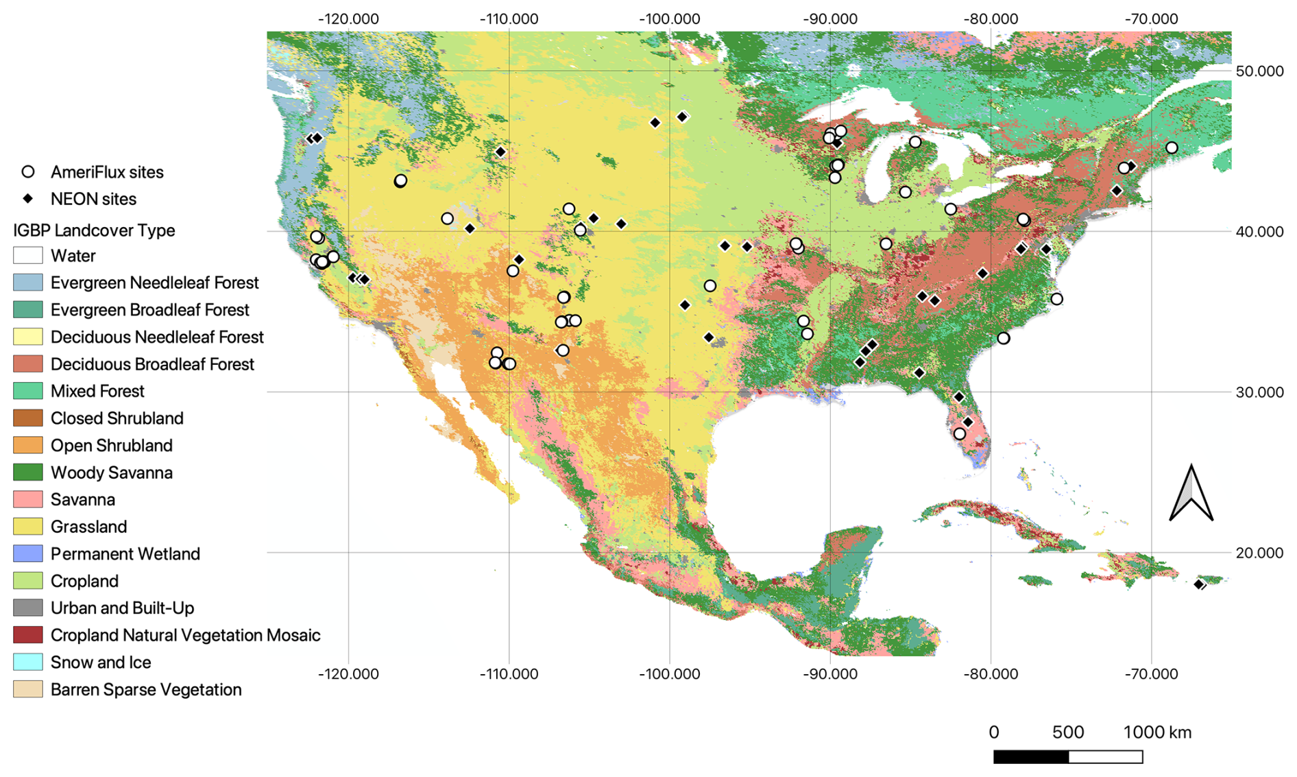
Figure 1 Locations of AmeriFlux and NEON sites used in this study, overlaid on the International Geosphere-Biosphere Programme (IGBP) land cover classification.

We used latent heat flux (LE) measured by the towers to estimate actual ET using Eq. (1) (Allen et al., 1998), which we used as the training target and in situ data for validation and testing.

$$\begin{array}{}\text{(1)}& \text{ET}={\displaystyle \frac{\mathit{LE}}{\mathit{\lambda }}}\end{array}$$

where λ is the latent heat of vaporization. Assuming a water density of 1000 kg m⁻³, this yields ET in mm per time. The latent heat of vaporization varies slightly with temperature and can be computed using Eq. (2) (Allen et al., 1998, 2006):

$$\begin{array}{}\text{(2)}& \mathit{\lambda }=\mathrm{2.501}-(\mathrm{2.361}\times {\mathrm{10}}^{-\mathrm{3}})\times T_{\mathrm{a}}\end{array}$$

Where T_a is air temperature in °C, and λ is in MJ kg⁻¹.

2.2 ABI observations from GOES-R satellite

We used the Level 2 Cloud and Moisture Imagery (CMI) observations and land surface bidirectional reflectance factor (BRF) products from the ABI aboard the GOES-16 satellite, which has been operational since November 2017. The ABI captures data across 16 spectral bands, spanning the visible, near-infrared (NIR), shortwave infrared (SWIR), and infrared (IR) wavelengths, with spatial resolutions ranging from 0.5 to 2 km at nadir, depending on the specific band (Table 1, Goodman et al., 2019; Khan et al., 2021; Schmit et al., 2017). The CMI product provides top-of-atmosphere observations whereas the BRF product offers atmospherically surface reflectance data for the reflective bands at visible, NIR and SWIR channels (BRF01, BRF02, BRF03, BRF05, BRF06, detailed in Table 1). The ABI provides full-disk imagery every 10 min and CONUS imagery every 5 min in its typical scan mode (Mode 6, Goodman et al., 2019; He et al., 2019). For our analysis, we synchronized ABI data from 2019 to 2022 with ground-based eddy covariance measurements from 94 AmeriFlux and NEON sites (Losos et al., 2024b) across the GOES-R CONUS scene.

Table 1 Summary of ABI bands and their primary uses (Schmit et al., 2017).

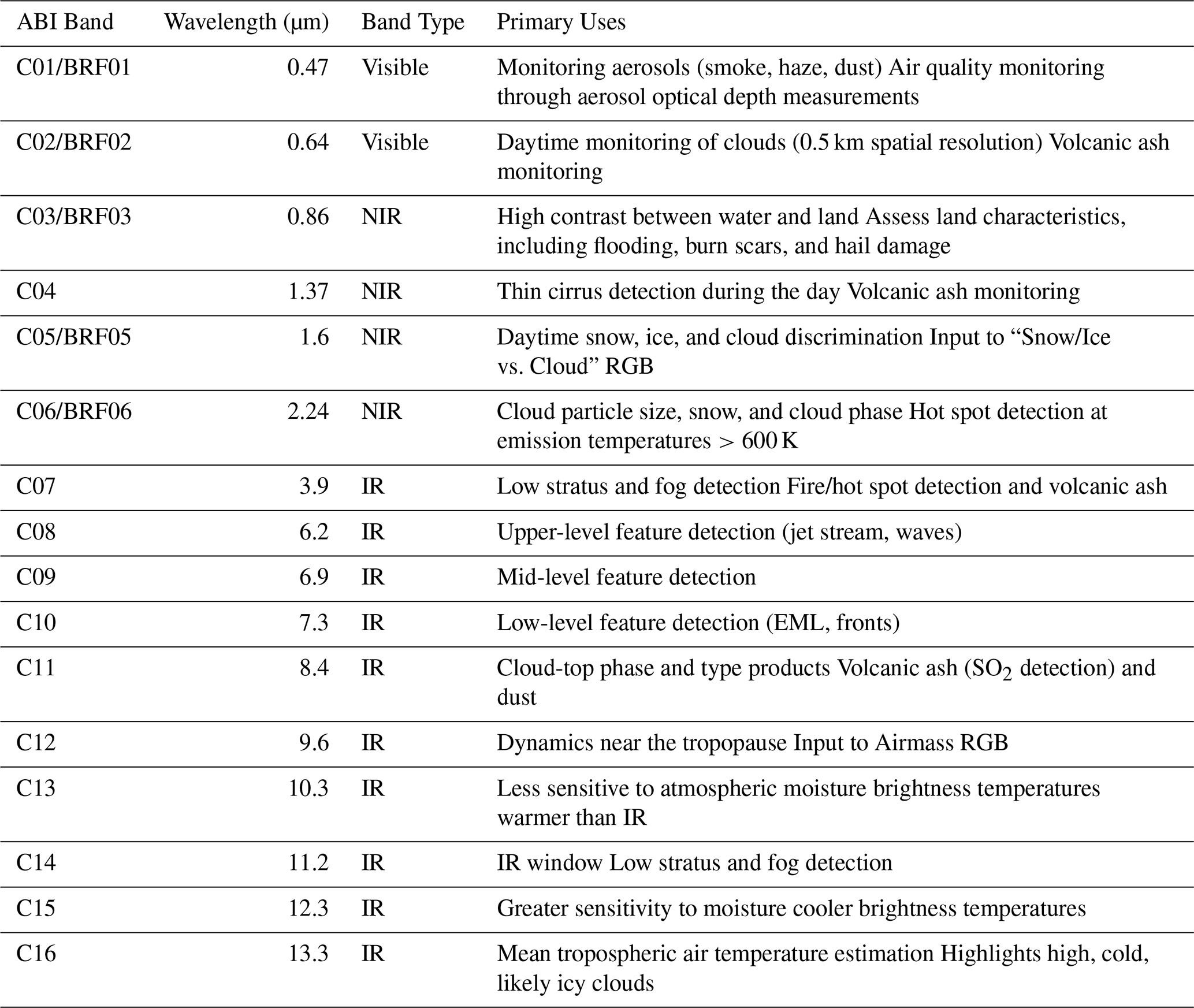
In addition to ABI observations, we incorporated Solar Zenith Angle (SZA) data, ALIVE-derived all-sky Downwelling Shortwave Radiation (ALIVE_DSR, Ranjbar et al., 2024d) and ALIVE-derived all-sky Land Surface Temperature (ALIVE_LST, Ranjbar et al., 2024b) estimates. From the BRF bands, we calculated the NIR reflectance of vegetation (NIRv, Dechant et al., 2022) and SWIR-enhanced NIRv (sNIRv, Ranjbar et al., 2024a) indices as proxies for vegetation productivity due to their strong correlation with canopy gross primary productivity and its strong relationship to ET. For the ET modeling, we used different configurations of variables for the daytime and nighttime. For nighttime, we focused on CMI bands along with SZA, ALIVE_DSR, ALIVE_LST, and the mean values of NIRv and sNIRv from the previous day (NIRv_daily_mean and sNIRv_daily_mean). For daytime, we included CMI, BRF, SZA, ALIVE_DSR, ALIVE_LST, NIRv, and sNIRv. We explored two feature strategies: one considering single real-time observations and another incorporating time series features from the previous 24 h.

To assess and validate the performance of our machine learning models, we compared against the physically-based Atmosphere-Land Exchange Inverse (ALEXI, Anderson, 1997) ET product into our analysis. ALEXI, developed with support from NASA, NOAA, and USDA ARS since 2003, estimates daily land-surface energy fluxes at a 5–10 km resolution using thermal infrared observations and vegetation indices from satellites. By combining a two-source (soil + canopy) energy balance model (TSEB; Norman et al., 1995) with an atmospheric boundary layer model, ALEXI provides accurate ET estimates under both clear and cloudy conditions (Anderson et al., 2007, 2012; Talib et al., 2021; Wanniarachchi and Sarukkalige, 2022). ALEXI is expanding globally through integration with international satellites, and it has been validated using flux tower data (RMSE of 35–40 W m⁻² at hourly time steps), making it a critical tool for ET and climate monitoring (Pan et al., 2020; Wanniarachchi and Sarukkalige, 2022; Zheng et al., 2022). To ensure consistency, we summed our ALIVE_ET estimates from the empirical machine learning approach to a daily scale to compare against the physically-based ALEXI (Sun et al., 2017).

2.3 Machine learning modeling and assessment

After synchronizing satellite-based observations and derived ALIVE_DSR and ALIVE_LST products with tower-based measurements, we used the tower-derived ET measurements (described in Sect. 2.1) as the target for estimation. Because eddy covariance observations are available at 30 min intervals, model training and validation were conducted at this temporal resolution, while the trained models were applied at the native 5 min GOES sampling frequency during inference. Daytime and nighttime samples were separated based on SZA to ensure a physically consistent classification across seasons and latitudes. For predictors, we utilized the satellite-based features outlined in Sect. 2.2 in two strategies. In the first, we considered the single-time observations at the time of measurement, while in the second, we incorporated time series features from the preceding 24 h. This introduces a temporal scale mismatch between training and application, and thus 5 min estimates should be interpreted as high-frequency interpolations constrained by half-hourly observations rather than independently validated predictions.

We applied two machine learning regression models: GBR and LSTM. GBR has demonstrated strong performance in estimating downwelling shortwave radiation (Ranjbar et al., 2024d), LST (Ranjbar et al., 2024b), and surface-atmosphere carbon dioxide flux (Ranjbar et al., 2024c), providing a balance between accuracy and computational efficiency for real-time applications. We compared GBR against LSTM, given its effectiveness with time series data (Dhake et al., 2023), which excels in capturing long-term dependencies in sequential data (Dhake et al., 2023; Hochreiter and Schmidhuber, 1997; Reddy and Prasad, 2018) which we felt may improve estimation of nighttime ET, for which soil evaporation is an important term, which itself is often modeled as a simple function of time since precipitation (Brutsaert, 2014).

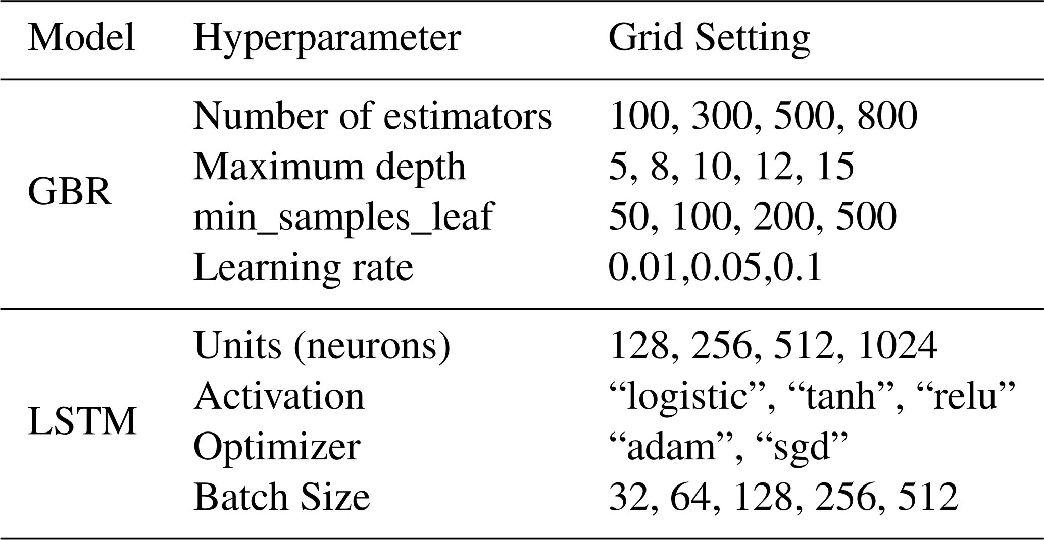
GBR is an ensemble learning model, refining predictions iteratively by optimizing a loss function through decision trees (Friedman, 2001). Key hyperparameters such as number of estimators, maximum depth, minimum samples per leaf, and learning rate influence the model's accuracy, complexity, and convergence speed (Bentéjac et al., 2021; Sahin, 2020). LSTM networks, designed for sequential data, utilize a memory cell architecture to address non-linear dependencies in time series forecasting (Ghanbari et al., 2021; Sutskever et al., 2014). Our LSTM architecture included two LSTM layers, followed by dense layers for feature extraction and output generation. The first LSTM layer retained the entire sequence (return_sequences=True), while the second layer summarized the learned information (return_sequences = False). The time series features in LSTM models are structured in a 3D input format, consisting of samples, time steps, and features. In contrast, since the GBR model accepts a 2D input, we explicitly included past values by incorporating the preceding 24 h of time series features as individual predictors, with each hour treated as a separate feature. Models were trained on Google Colab Pro (32 GB RAM, A100 GPU) using a grid search algorithm to optimize hyperparameters for correlation determination (R²) and prediction time (P.T., see Table 2 for grid search specifications and hyperparameter settings). Model inference, particularly for the GBR configuration, occurs on the order of seconds per domain and is suitable for near real-time applications, while the higher computational cost reported primarily reflects LSTM training rather than operational deployment.

Table 2 Grid search specifications and hyperparameter setting for machine learning models.

For validation, we applied Leave-One-Out Cross-Validation (LOOCV), reserving 20 % of eddy covariance sites for testing while training on the remaining sites using a four-fold cross-validation (75:25 training-validation split) (Maxwell et al., 2018). This procedure was repeated ten times with different random seeds to enhance robustness and minimize bias. Final results, including correlation determination (R², Eq. 3), root mean square error (RMSE, Eq. 4), and normalized RMSE (nRMSE, Eq. 5) were averaged to ensure reliability, using the Scikit-learn Python library (Pedregosa et al., 2011).

$$\begin{array}{}\text{(3)}& R^{\mathrm{2}}=\mathrm{1}-{\displaystyle \frac{\text{RSS}}{\text{TSS}}},\end{array}$$

where RSS is the sum of squares of residuals and TSS is the total sum of squares.

$$\begin{array}{}\text{(4)}& {\displaystyle }\text{RMSE}=\sqrt{{\displaystyle \frac{\sum _N^{i=\mathrm{1}}(x_i-\widehat{x})}{N}}},\text{(5)}& {\displaystyle }\text{nRMSE}={\displaystyle \frac{\text{RMSE}}{x_{\mathrm{med}}}},\end{array}$$

where x_med is the median of the observations, i variable i, N is the number of non-missing data points, x_i are actual observations in the time series, and $\widehat{x}$ is the estimated time series.

To interpret model behavior, we used SHAP (Shapley Additive Explanations), a game-theoretic approach that quantifies the contribution of each input feature to individual predictions (Lundberg and Lee, 2017). SHAP values represent the marginal impact of a feature relative to a baseline prediction, allowing consistent comparison of feature importance across models and conditions (An et al., 2026; Ranjbar, 2025).

3 Results

3.1 Model Performance for ALIVE_ET Estimates

Table 3 and Fig. 2 illustrate the performance of LSTM and GBR models in estimating half-hourly (hh) ALIVE_ET compared to EC-derived ET under daytime and nighttime conditions. During the daytime (Fig. 2a), the GBR model outperformed LSTM when using single-time features, achieving the highest R² (0.74) and the lowest nRMSE (0.91). Incorporating time series features improved the LSTM model's performance (R² of 0.72 and nRMSE of 1.05), making it comparable to the GBR model (R² of 0.71 and nRMSE of 1.16). While the LSTM model benefits significantly from GPU acceleration, leveraging the A100 GPU (40/80 GB VRAM, Tensor Cores, High Throughput) in Google Colab Pro (32 GB RAM) to reduce training and inference time, it remains computationally expensive. The GBR model, on the other hand, primarily runs on the CPU and does not gain performance boosts from GPU acceleration. Even with GPU acceleration, the LSTM model still requires 5.3 times more computation time than GBR and fails to surpass GBR in modeling accuracy for daytime ET estimation. At night (Fig. 2b), GBR model performance was notably lower and the LSTM model, trained on time series features, performed better (R² of 0.24 and nRMSE of 1.29 versus GBR R² of 0.21 and nRMSE of 1.78).

Table 3 Performance metrics (R², nRMSE, and prediction time (P.T.)) of LSTM and GBR models for half-hourly (hh) ALIVE_ET vs. EC-derived ET for daytime and nighttime estimates. T indicates relative prediction time compared to the GBR model using single daytime features. Metrics are computed on a site-independent test set, where 20 % of eddy covariance sites are withheld from training. Best performances for night and day are bolded.

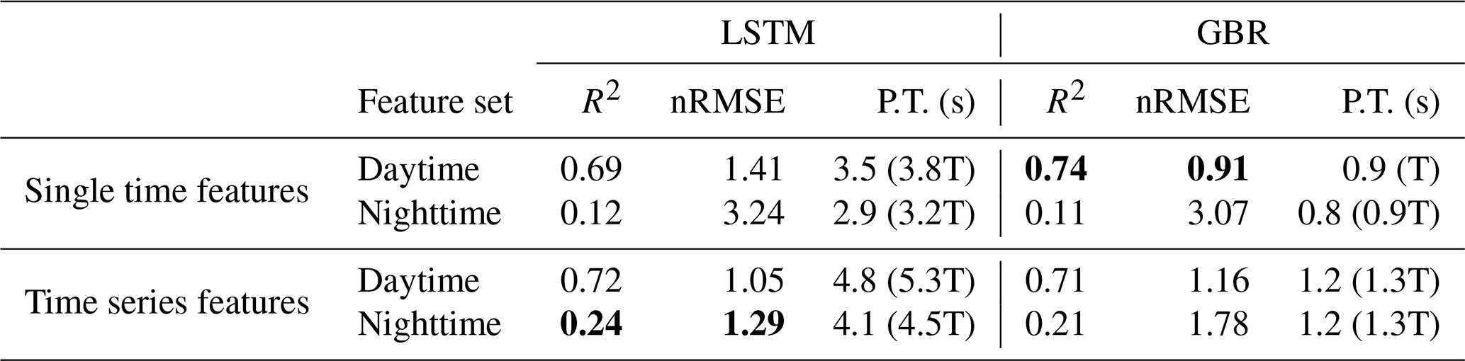
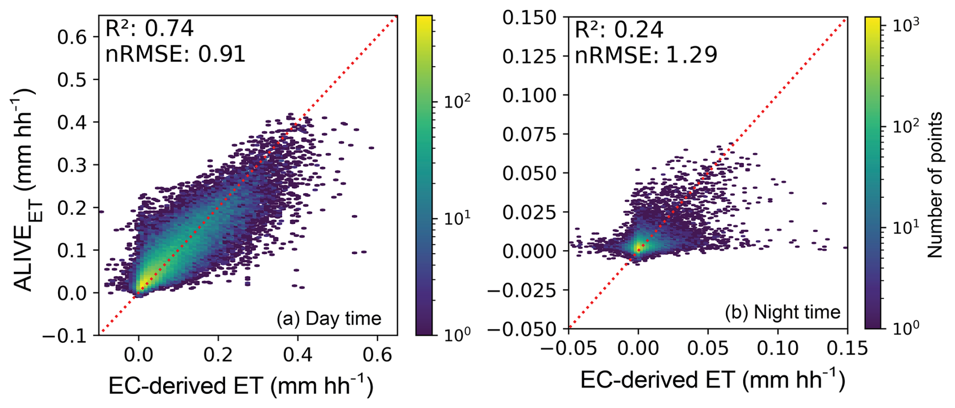
Figure 2 Density scatter plots of EC-derived ET (mm half-hourly⁻¹) (a) vs. daytime ALIVE_ET estimated from GBR trained on single time observations (n=17 480) and (b) nighttime ALIVE_ET estimated from LSTM trained on time series observations (n=14 304).

To further evaluate the all-sky capability of the ALIVE_ET framework, model performance was stratified by clear-sky and cloudy-sky conditions based on the GOES cloud mask classification (Table A3). During daytime, the GBR model maintained strong performance under clear-sky conditions (R²=0.77; nRMSE = 0.73), while performance decreased under cloudy conditions (R²=0.63; nRMSE = 1.81), reflecting the increased uncertainty associated with cloud-contaminated radiative signals. A similar pattern was observed at night for the LSTM model, with comparable R² values under clear (0.24) and cloudy (0.21) conditions, but a noticeable increase in nRMSE under cloudy skies (1.03 vs. 2.06).

3.2 Model performance in representing diurnal dynamics and seasonal variability

Figure 3 demonstrates the ALIVE_ET model's capability to capture mean, across-site diurnal variations in ET by comparing its estimates with EC-derived ET across different local hours for both daytime and nighttime conditions. Values are averaged across all sites for each local hour. During the daytime, the model exhibits strong agreement with observed ET. ET values rise in the morning, peak around midday, and gradually decline in the afternoon, closely mirroring the EC-derived ET trend. However, during nighttime, ET values drop significantly due to the absence of solar radiation, and while the model captures some fluctuations, biases from EC-derived ET are more noticeable.

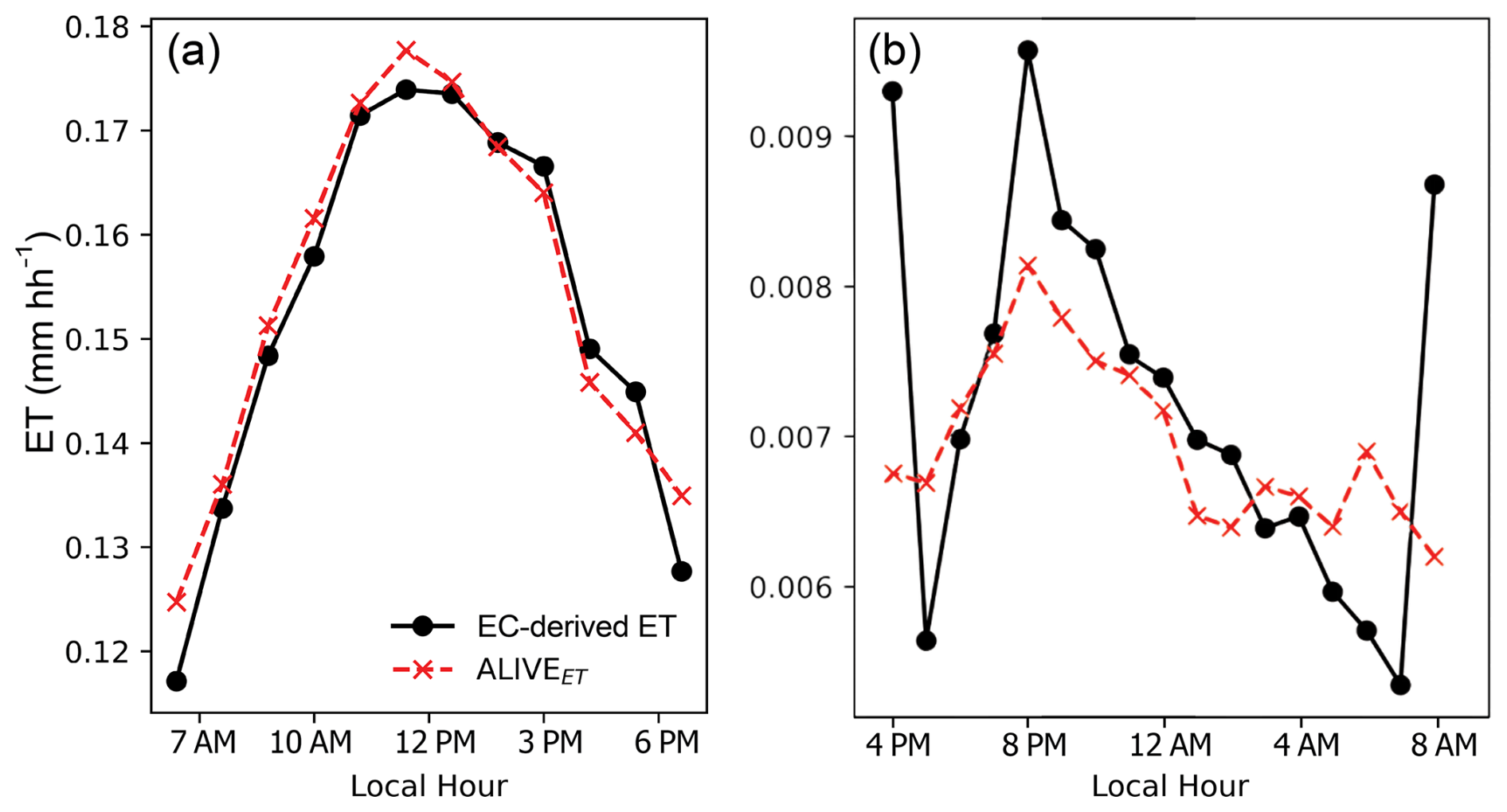
Figure 3 Mean values of EC-derived ET (mm half-hourly⁻¹) (a) vs. daytime ALIVE_ET estimated from GBR trained on single time observations and (b) nighttime ALIVE_ET estimated from LSTM trained on time series observations. Values are hourly averages derived from 30 min data and are averaged across all sites for each local solar hour, with daytime and nighttime defined based on SZA.

Figure 4 evaluates the model's performance across different months in 2023, with metrics averaged across all sites. The R² follows a distinct seasonal pattern, with lower values during late winter and early spring, and improved performance from May to September. Additionally, the seasonal trend in LST, a key predictor variable, aligns with model performance, as warmer months exhibit more accurate ET estimates while colder months introduce greater uncertainty. Figure 4c shows the one year time series of daily ALIVE_ET estimates against calculated ET from EC measurements (EC-derived ET), which shows the model's robustness, with an annual R² of 0.99 and nRMSE of 0.64.

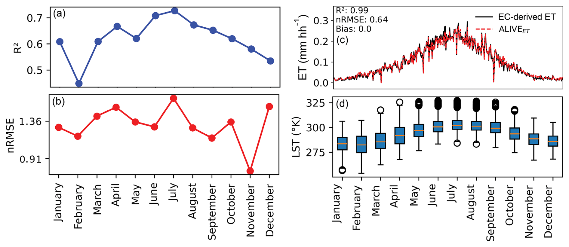
Figure 4 Model performance across different months: (a) R² values, (b) nRMSE values, (c) model fit for mean daily ET (mm  half-hourly⁻¹) over the entire year of 2023, and (d) LST distribution showing monthly variability with boxplots.

3.3 Feature importance

For daytime ET modeling (Fig. 5c), the most influential feature is NIRvP, followed by ALIVE_LST and sNIRvP. Other important predictors include ALIVE_DSR, CMI_C03 (top-of-atmosphere NIR at 0.86 µm), and BRF5 (surface SWIR reflectance at 1.6 µm). SHAP values indicate that higher NIRvP and ALIVE_LST values positively affect ET predictions, underscoring the importance of thermal and vegetation-related features. Lower-ranked features, such as CMI_C04 and BRF3, have minimal impact on prediction, a point that is further discussed in the discussion section.

For nighttime ET modeling (Fig. 5a), a different set of predictors emerges, with ALIVE_LST, sNIRv_daily_mean, and NIRv_daily_mean standing out as the most dominant variables. Unlike the daytime model, the absence of the surface reflectance product and DSR values near or equal to zero shifts the focus toward top-of-atmosphere SWIR and thermal observations. The lower SHAP values associated with specific CMI variables, such as CMI_C09 and CMI_C08, indicate that these spectral bands have less influence on nighttime ET estimation compared to other variables. Additionally, the time series analysis in Fig. 5b emphasizes the significance of remote sensing observations taken 2 and 4 h before the ET prediction. In contrast, observations from 12 to 18 h prior to ET have the least influence, while those from 22 to 24 h also gain some importance.

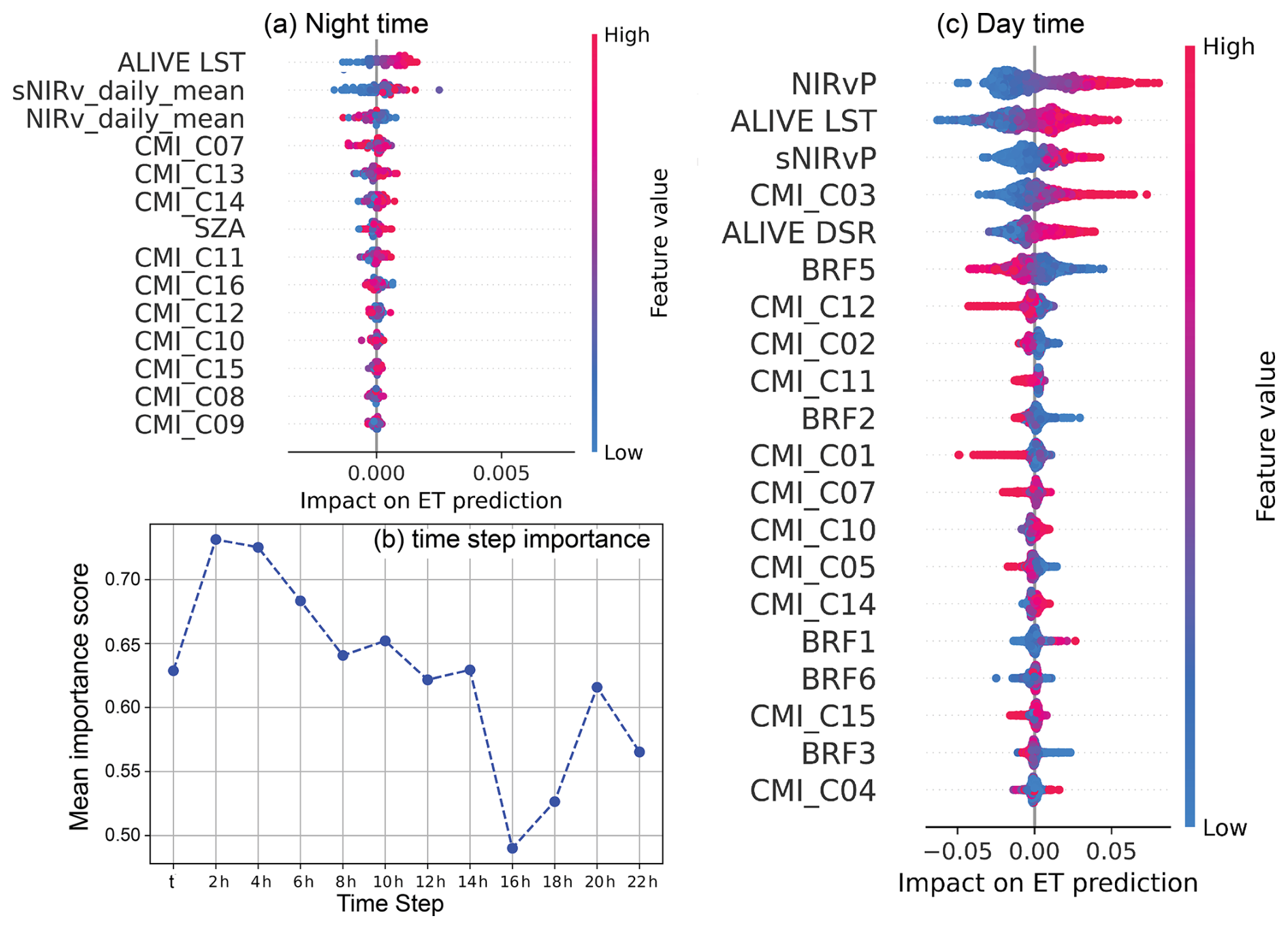
Figure 5 Feature importance analysis using SHAP values for (a) nighttime, (b) nighttime time-step importance, and (c) daytime. Panels (a) and (c) rank the top features by importance for nighttime and daytime, respectively, while (b) highlights time-step importance in the nighttime model, where the LSTM with time series features performed best.

3.4 Model Performance Across different Köppen climate classes and IGBP vegetation covers

We evaluated the model's performance across different Köppen climate classifications (Figs. 6 and A1) and IGBP land cover types (Figs. 7 and A2) by comparing ALIVE_ET estimates with EC-derived ET. We averaged the site-level estimates within each climate classification or land cover type. For this analysis, we focused on the five most prevalent climate types covering the largest land areas across CONUS for discussion, while results for all climate types are presented in the figures. The Fig. 6 left panels display density scatter plots comparing half-hourly ALIVE_ET estimates to EC-derived ET, while the right panels illustrate daily time series for the years 2022 and 2023.

Across different climate zones, ALIVE_ET demonstrates varying levels of agreement with EC-derived ET. In Mediterranean climates (Csa/Csb), the model shows moderate-to-strong performance, with half-hourly R² values of 0.68 (Csa) and 0.58 (Csb), increasing to 0.86 and 0.81 at the daily scale, respectively. Similarly, in humid subtropical (Cfa) and humid continental (Dfb/Dfa) climates, ALIVE_ET performs well, with half-hourly R² values ranging from 0.67 to 0.75 and daily R² values between 0.86 and 0.91, indicating strong consistency in capturing daily ET dynamics. The nRMSE remains relatively low across these regions, generally ranging from 0.56 to 1.46 at the daily scale. In drier climates, performance slightly declines. In semi-arid steppe (Bsk) regions, ALIVE_ET maintains reasonable agreement, with R² values of 0.57 at the half-hourly scale and 0.78 at the daily scale, accompanied by modest increases in nRMSE. The lowest agreement is observed in arid desert (Bwk) climates, where half-hourly R² decreases to 0.48 and daily R² to 0.73, and nRMSE reaches its highest values, reflecting increased uncertainty under strongly water-limited conditions.

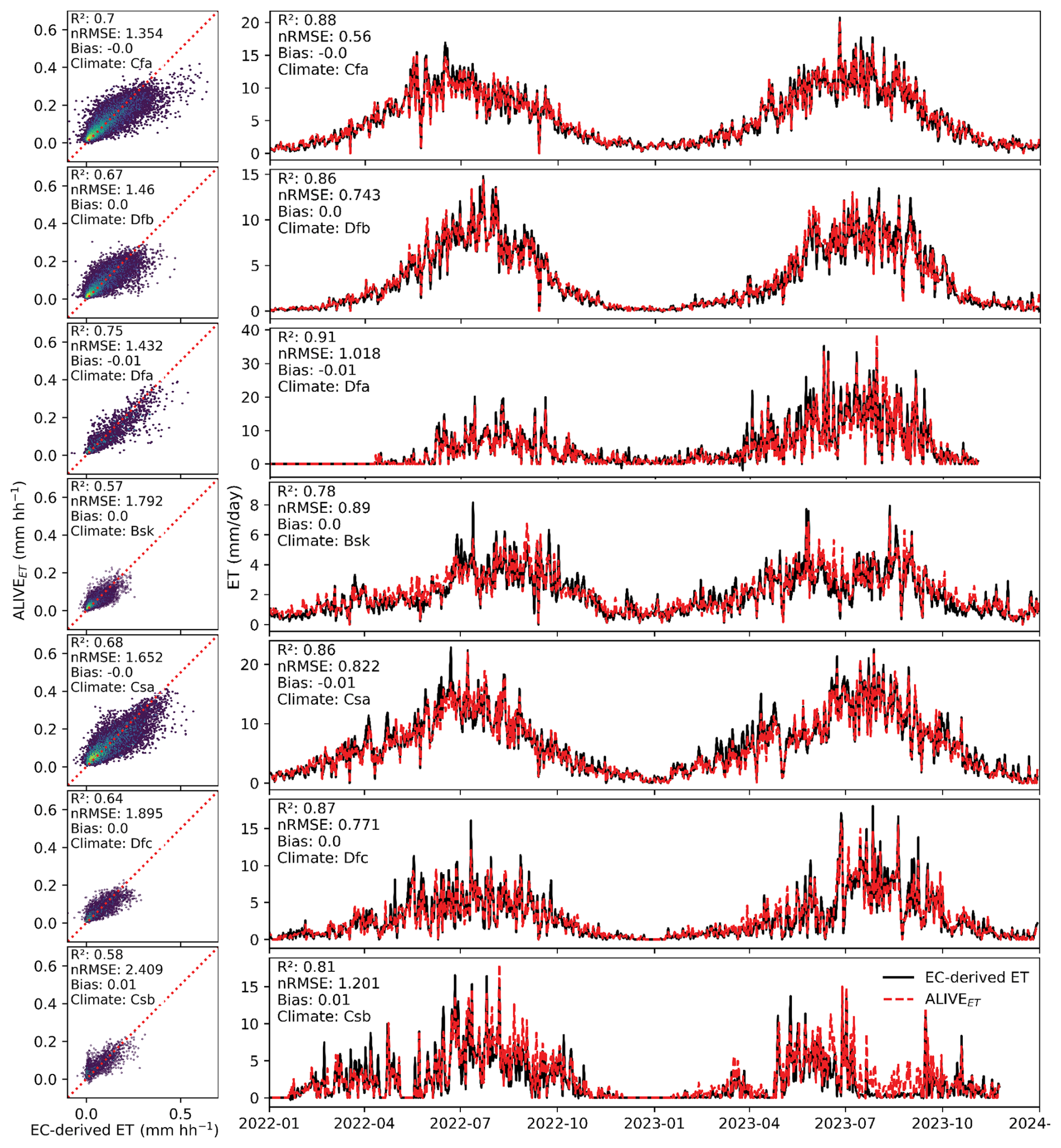
Figure 6 ALIVE_ET estimates compared to EC-derived ET across different Köppen climate classes (see Table A2 in the appendix for climate class full name). Left panels display density scatter plots of half-hourly estimates, while right panels show daily time series of ALIVE_ET vs. EC-derived ET for 2022 and 2023. Results represent aggregated statistics across all sites within each climate class.

Figures 7 and A2 present a comparative evaluation of ALIVE_ET estimates against EC-derived ET across different land cover types classified according to the IGBP. Similar to Fig. 6, the left panels illustrate density scatter plots of half-hourly ET estimates, while the right panels depict daily time series comparisons for 2022–2023. Performance varies across land cover types. Wetlands (WET) exhibit strong agreement, with a half-hourly R² of 0.77 and an nRMSE of 1.23, increasing to a daily R² of 0.92 and an nRMSE of 0.73, indicating robust skill in capturing both sub-daily variability and seasonal dynamics. Grasslands (GRA) and croplands (CRO) also show relatively high agreement, with half-hourly R² values of 0.78 and 0.66, and daily R² values of 0.90 and 0.84, respectively. Forested ecosystems, including deciduous broadleaf forests (DBF) and evergreen needleleaf forests (ENF), demonstrate moderate-to-strong performance, with daily R² values of 0.89 and 0.85, respectively. In contrast, evergreen broadleaf forests (EBF), savannas (SAV), and barren or sparsely vegetated (BSV) regions exhibit lower agreement, with half-hourly R² values of 0.48, 0.27, and 0.36, respectively (Fig. A2), and increased nRMSE, reflecting reduced predictive skill in these ecosystems, which are less represented in the EC tower network. The time series comparisons further highlight the temporal consistency between ALIVE_ET (dashed red) and EC-derived ET (black), particularly for WET, GRA, and CRO, where seasonal cycles and peak ET magnitudes are well captured. In contrast, BSV and SAV show larger discrepancies, with ALIVE_ET exhibiting greater variability and increased uncertainty during peak ET periods.

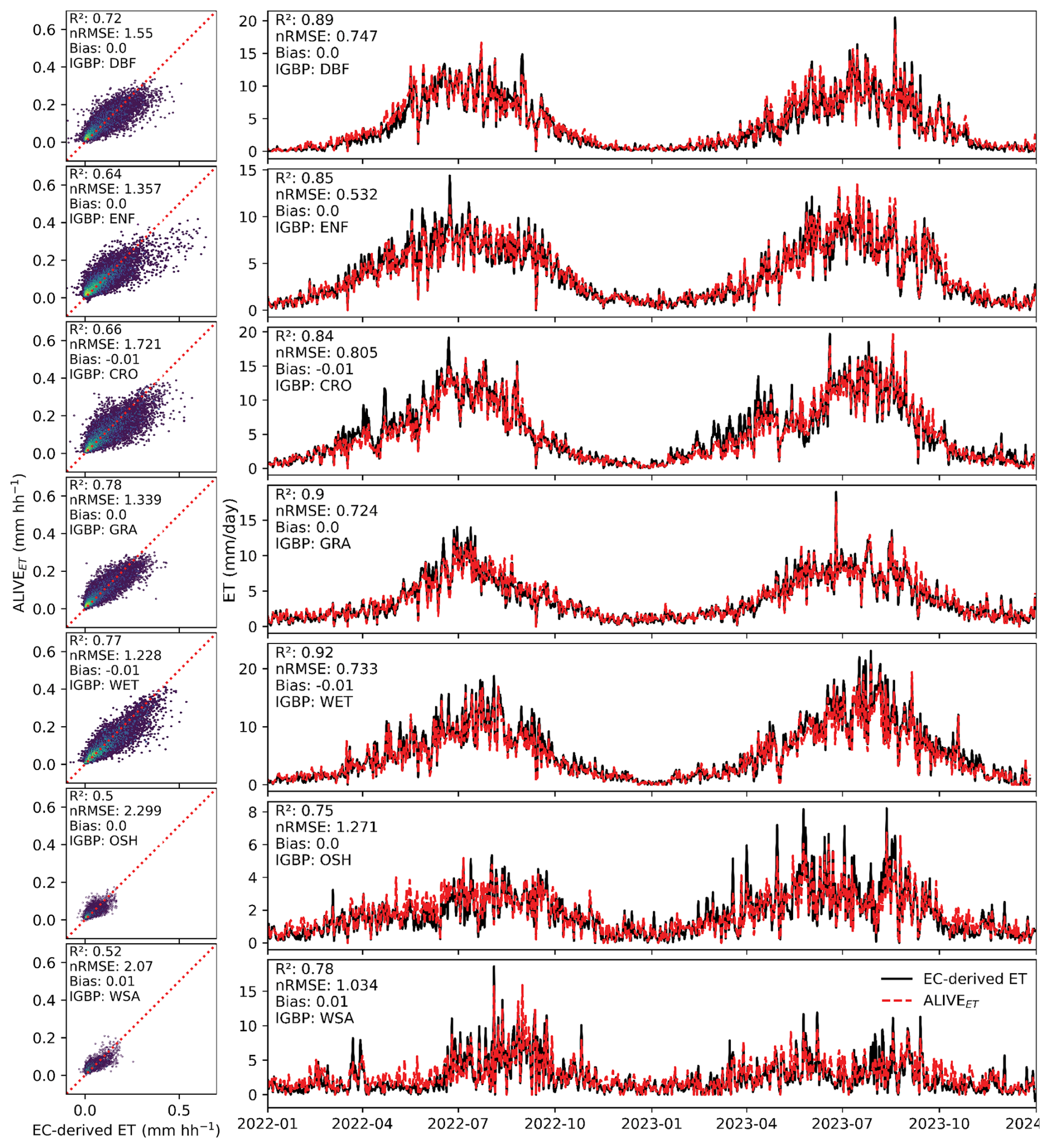
Figure 7 Comparison of ALIVE_ET estimates with EC-derived ET across different IGBP land cover types (see Table A2 in the appendix for full name). Left panels show density scatter plots of half-hourly estimates, while right panels display daily time series of ALIVE_ET vs. EC-derived ET for 2022 and 2023. Results represent aggregated statistics across all sites within each land cover class.

3.5 Comparing ALIVE_ET against ALEXI

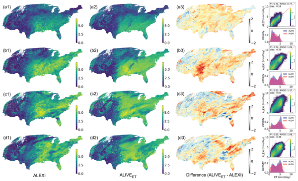
To assess the performance of the ALIVE_ET model across space, we compared its daily aggregated ET estimates against those derived from the physically-based ALEXI model. We selected 4 d (DOY 117, 149, 179, and 218) from mid-May to mid-August 2022, ensuring a minimum 30 d interval between them for a spatial and statistical comparison. These days were chosen based on minimal cloud cover to ensure a fair comparison between the ET estimations. Since ALEXI estimates ET under cloudy conditions using post-processing techniques, selecting clear-sky days allows for a more direct evaluation of the models without the influence of these adjustments. The first and second columns in Fig. 8 illustrate the spatial distributions of ALEXI and ALIVE_ET, respectively, while the third column depicts their differences (ALIVE_ET – ALEXI) alongside density scatter plots and kernel density estimates (KDE).

ALIVE_ET exhibits strong agreement with ALEXI across different regions and time periods, capturing similar spatial patterns of ET variability. However, noticeable differences emerge in certain areas, particularly in the central and eastern United States, where ALIVE_ET estimates are generally lower than ALEXI (Fig. 8, Column 3). These differences are more pronounced on DOY 149 and 179, where negative biases dominate, suggesting potential underestimation of ALIVE_ET relative to ALEXI in regions with relatively high vegetation density.

The density scatter plots indicate a generally strong correlation between ALIVE_ET and ALEXI, with R² ranging from 0.62 to 0.74. RMSE values vary between 0.77 and 1.17 mm d⁻¹, with biases fluctuating between −0.16 and −0.67 mm d⁻¹ (about 2.8 % to 11.9 % relative to the median ALEXI). These values highlight a consistent but slightly underestimated ET prediction by ALIVE_ET that we discuss further in the Discussion section. The KDE histograms further reveal that ALIVE_ET and ALEXI share similar ET distributions, though ALIVE_ET exhibits a higher density of lower ET values, which may be attributed to differences in model parameterizations or the input data utilized by the machine learning framework.

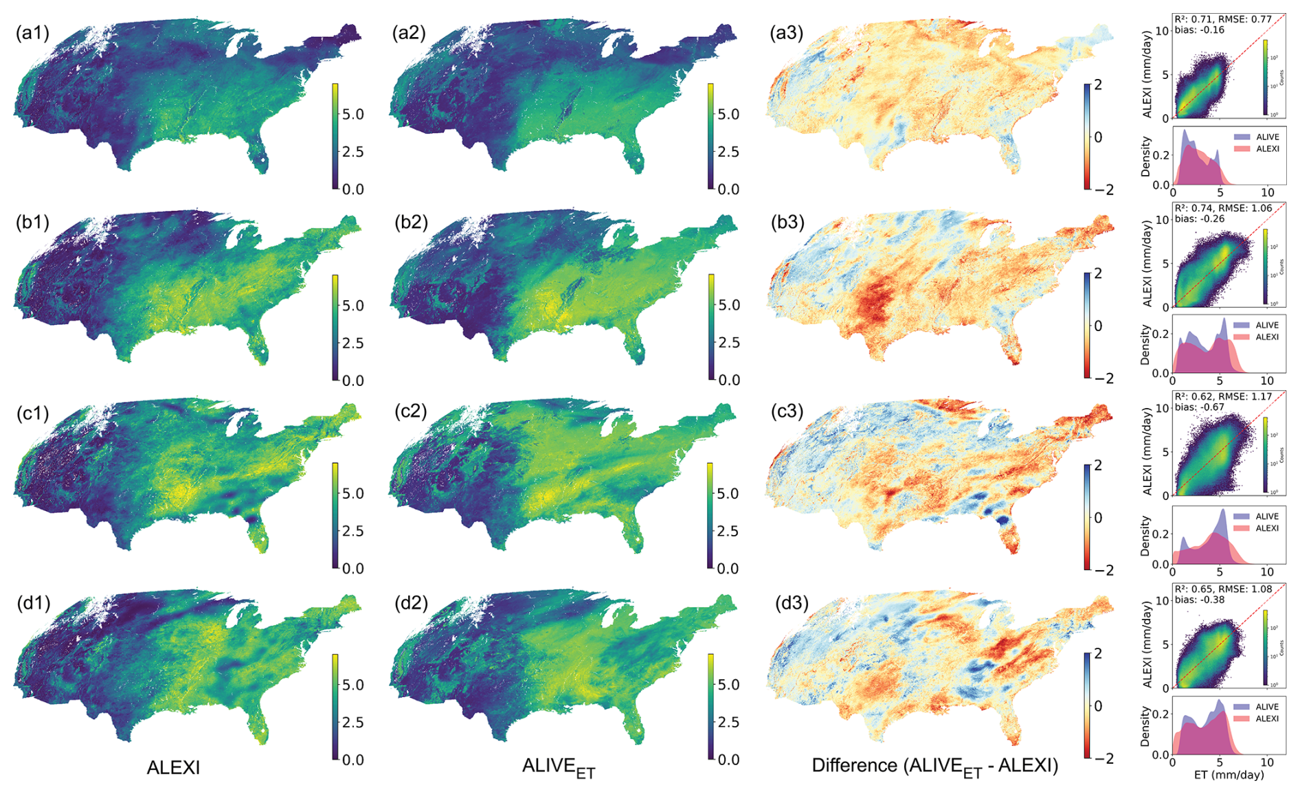
Figure 8 Comparison of daily ET estimates from ALEXI and ALIVE. Column 1 shows ALEXI_ET maps, Column 2 presents ALIVE_ET maps, and Column 3 displays their differences in units of mm d⁻¹, along with density scatter plots and KDE histogram distributions. Days of the year (DOY) with the lowest cloud cover, selected from mid-May to mid-August in 2022, include (a) 117, (b) 149, (c) 179, and (d) 218.

4 Discussion

4.1 Model Performance for ALIVE_ET Estimates

The comparative analysis of GBR and LSTM models in estimating ALIVE_ET reveals a clear trade-off between predictive accuracy, computational efficiency, and adaptability to near real-time half hourly estimation. GBR outperforms LSTM during daytime, likely due to its ability to model nonlinear interactions without requiring sequential dependencies (Bentéjac et al., 2021; Dhake et al., 2023; Sahin, 2020). GBR efficiently captures the relationship between solar radiation, temperature, and vegetation indices, providing accurate estimates of daytime ET with minimal computational cost. LSTM, despite its capability to model temporal dependencies, fails to improve predictions. The computational burden of LSTM further limits its practicality for large-scale, near real-time applications (Ranjbar et al., 2024d). It is important to note that eddy covariance measurements used for training and validation contain inherent uncertainties, particularly due to energy balance non-closure; no additional closure correction was applied here to avoid introducing site-specific assumptions that could bias cross-site consistency, and forcing closure introduces additional assumptions such that it is not recommended at the site or network scale (Leuning et al., 2012; Mauder et al., 2024).

At night, both models struggle, reflecting the inherent challenges of predicting nocturnal ET that is most strongly related to environmental drivers that are difficult to discern from space, namely near-surface wind speed and vapor pressure deficit as well as air temperature (Fisher et al., 2007; Novick et al., 2009). The absence of direct solar radiation reduces variability, making it difficult for data-driven models to learn meaningful patterns. LSTM exhibits a slight advantage over GBR, possibly due to its ability to capture residual heat flux and time since CMI observations that are consistent with precipitation events through the sequential dependencies in time series data (Dhake et al., 2023; Ghimire et al., 2022). However, this improvement remains marginal, indicating that neither model fully accounts for the complex boundary layer processes governing nighttime ET and challenges measuring it with eddy covariance. Nighttime ET remains particularly uncertain due to low signal-to-noise ratios and intermittent turbulence, and the relatively low R² values reflect both observational uncertainty and the weak magnitude of nocturnal fluxes rather than solely model deficiency. Incorporating other data sources for meteorological and soil parameters, such as humidity gradients and soil heat flux, could improve performance (Katul et al., 2012; Walker et al., 2019; Wanniarachchi and Sarukkalige, 2022). Cloud cover further reduces model performance, as reflected by higher errors under cloudy conditions, likely due to increased uncertainty in radiative inputs; however, the model retains skill under both conditions, supporting its applicability for all-sky ET estimation. Despite these limitations, including nighttime conditions provides a stringent test of the model's ability to resolve weak but non-zero evaporative processes at sub-daily scales.

These results show the importance of aligning model choice with application constraints. GBR is more suitable for real-time ET monitoring due to its efficiency, while LSTM, despite its potential for sequential modeling, remains limited by high computational costs (Ranjbar et al., 2024d). A promising direction is the development of hybrid models that leverage GBR's efficiency for daytime ET and LSTM's temporal learning for nocturnal predictions. Additionally, integrating physical constraints into machine learning models could enhance reliability, reducing dependence on purely empirical learning. Future work should explore attention-based architectures as a computationally efficient alternative to LSTM for capturing temporal dependencies in nocturnal ET estimation and seek to incorporate meteorological datasets, like the High Resolution Rapid Refresh (HRRR) (Dowell et al., 2022; James et al., 2022), to better simulate the meteorological processes that control ET.

4.2 Model performance in representing diurnal dynamics and seasonal variability

The ALIVE_ET model effectively captures diurnal ET dynamics, closely mirroring the expected daytime trend, rising in the morning, peaking at midday, and declining in the afternoon. This alignment with observed patterns is largely due to the model's empirical, data-driven nature, which leverages statistical relationships between environmental variables and ET (Angelov and Gu, 2019; Belitz and Stackelberg, 2021; Brunton and Kutz, 2022). However, its reliance on mean values across sites limits its adaptability to local-scale variations, potentially leading to oversimplifications in heterogeneous landscapes (Brunton and Kutz, 2022).

At night, biases become more pronounced, with ET values dropping sharply in the absence of solar radiation. While the model captures some nocturnal fluctuations, it struggles to estimate early morning and late afternoon transitions accurately. This challenge likely stems from reduced variability in key input features (Angelov and Gu, 2019), such as LST and radiation, which dominate ET estimation during daylight but provide weaker predictive signals at night. Eddy covariance data need to be filtered during periods of low turbulent intensity, which occur disproportionately in the early evening when turbulence is often suppressed (Van Gorsel et al., 2007). Standard quality control procedures, including friction velocity (u^*) filtering, were applied to reduce biases associated with low-turbulence conditions, though residual uncertainty remains. In addition to limitations in eddy covariance measurements, addressing this limitation to ML modeling requires integrating additional environmental drivers, such as humidity, soil moisture, and boundary layer meteorology, to better characterize latent heat exchange under low-energy conditions (Katul et al., 2012; Talib et al., 2021).

Seasonally, the model performs better during warmer months (May to September) and exhibits reduced accuracy in colder months. This trend reflects the direct relationship between LST and ET, where higher temperatures correspond to increased evaporative demand and more stable model predictions due to higher ET variability. In contrast, winter months introduce uncertainty due to lower LST values, as well as reductions in ET activity (Chen and Liu, 2020; Ling et al., 2022) and challenges posed by melting snow. The model's robustness at the annual scale, indicated by high R² for daily ET estimates, suggests it effectively generalizes long-term ET trends despite seasonal variations.

4.3 Feature importance

During daytime, vegetation-related and thermal features, particularly NIRvP and ALIVE_LST, emerge as the most influential predictors, reinforcing the strong dependence of ET on plant activity and temperature (Chen and Liu, 2020; Sun et al., 2012). The high SHAP values for NIRvP suggest that increased photosynthetic activity, as captured by red absorption and NIR reflectance, leads to higher ET rates (Zheng et al., 2022). Other relevant predictors, such as ALIVE_DSR and CMI_C03, contribute by incorporating solar radiation and top-of-atmosphere near-infrared signals. The lower SHAP importance of ALIVE_DSR reflects feature redundancy rather than reduced physical relevance, as radiation effects are partially captured by correlated variables such as ALIVE_LST; SHAP values represent marginal contributions within the feature set. BRF3 is utilized in the computation of NIRvP and sNIRvP, both of which are key predictors in the model. Therefore, BRF3 is assigned a lower importance ranking, which is a characteristic outcome of machine learning models when handling highly correlated input features. In such cases, the model prioritizes the most informative variable while diminishing the influence of redundant features to optimize predictive performance (Angelov and Gu, 2019; Brunton and Kutz, 2022).

In contrast, the best nighttime ET estimation was achieved from time series features using LSTM modeling. The model was primarily driven by surface temperature and the mean value of vegetation indices (NIRv and sNIRv) from prior day rather than instantaneous radiation inputs. ALIVE_LST remains the dominant predictor, aligning with the idea that nighttime ET is primarily governed by residual surface heat and micrometorological variables like wind, temperature, and atmospheric dryness rather than direct solar-driven processes (McColl, 2020; Wanniarachchi and Sarukkalige, 2022). The significance of daily-averaged vegetation indices (sNIRv_daily_mean and NIRv_daily_mean) indicates that plant water loss continues into the night, albeit at much lower magnitudes, influenced by prior daytime conditions. Unlike daytime modeling, DSR is absent as a predictor, leading to increased reliance on CMI observations in the thermal infrared.

Furthermore, the time-step analysis for nighttime modeling highlights the temporal dependencies within the LSTM framework. Observations from 2 to 4 h before the prediction time contribute the most, emphasizing the short-term persistence of environmental signals in driving nighttime ET. Conversely, observations from 12 to 18 h prior show minimal influence, likely due to the decoupling of past daytime energy inputs. Interestingly, inputs from 22 to 24 h earlier gain some relevance, potentially capturing the effects of previous nighttime cooling trends or delayed surface moisture responses (Labedzki, 2011) but also consistent with correlation amongst nighttime conditions. These findings highlight the need for tailored ET models, with nighttime models relying on time-series features, particularly LST and indices, while daytime models benefit from instantaneous reflectance, solar inputs, and LST. Future improvements could involve adding new features, particularly for nighttime ET, where additional environmental variables might enhance predictive accuracy (Fisher et al., 2007; Katul et al., 2012; Novick et al., 2009; Walker et al., 2019).

4.4 Model Performance Across different Köppen climate classes and IGBP vegetation covers

The varying performance of ALIVE_ET across climate classifications and land cover types highlights the inherent challenges in modeling ET in diverse environmental conditions. The strong performance in Mediterranean (Csa/Csb) and humid subtropical (Cfa) climates suggests that the model effectively captures ET dynamics in regions with consistent seasonal cycles and climate-driven vegetation dynamics (Feng et al., 2019; Zhou et al., 2021). This is likely because these climates exhibit strong and stable relationships between radiation, temperature, and vegetation indices, which are key drivers of ET (Feng et al., 2019; Labedzki, 2011). These patterns should be interpreted in the context of the training dataset, which is limited to CONUS flux tower sites and does not fully represent all global land cover types. Climate classes that are sampled less, like Mediterranean climates, present additional complexity due to pronounced shifts between energy-limited and water-limited periods within the same year (Ryu et al., 2008), where ET dynamics are strongly modulated by seasonal soil moisture availability. The strong seasonal greenness signal and surface temperature variability in these regions may enhance the ability of machine learning models to capture ET dynamics.

However, the accuracy of ALIVE_ET declines in more arid regions such as semi-arid steppe (Bsk) and arid desert (Bwk) climates. The higher errors in these environments can be attributed to the increased influence of soil evaporation, sparse vegetation cover and its subgrid variability, the pronounced spatial heterogeneity of these ecosystems, and the episodic nature of precipitation, all of which introduce greater variability in ET rates (Krishnan et al., 2012; Tabari et al., 2012). The model's reliance on vegetation indices and thermal features may lead to oversimplifications in these water-limited regions, where plant water use efficiency and soil moisture interactions play crucial roles in governing ET.

Another critical factor affecting model performance in drier climates is the role of advection and non-local energy sources. ET is not solely controlled by local surface conditions but is also influenced by large-scale atmospheric dynamics and horizontal energy transport, factors that are difficult to capture using data-driven models based on local predictors (Krishnan et al., 2012; Pan et al., 2020; Weiß and Menzel, 2008). Furthermore, the increased nRMSE in these regions suggests that the model may struggle with capturing sub-daily variability, particularly in conditions where rapid changes in atmospheric demand or soil moisture availability occur. Future enhancements may involve integrating soil moisture retrievals, atmospheric boundary layer dynamics, or explicitly accounting for advection by incorporating upstream pixels in the model training process to improve performance in these challenging regions.

The land cover analysis reveals similar challenges. While the model performs well in wetlands (WET), grasslands (GRA), and croplands (CRO), it struggles in evergreen broadleaf forests (EBF), savannas (SAV), and barren or sparsely vegetated (BSV). The strong performance in wetlands can be attributed to the dominance of surface water evaporation, which is well captured by thermal and vegetation indices (Bao et al., 2021; Drexler et al., 2004; Fleischmann et al., 2023). In contrast, the lower R² values in BSV and SAV suggest that canopy structure, water use strategies, and plant functional diversity introduce complexity that is not adequately represented by the current feature set (Liu et al., 2022; Pan et al., 2024), and there are currently few measurements in the CONUS scene with which to train models (Figure 1). The reduced performance in SAV and EBF is therefore likely driven by limited representation in the training data rather than fundamental limitations of the modeling approach. Dense canopies in EBF likely lead to discrepancies between surface temperature and actual transpiration rates, as the thermal signal captured by satellites may not directly reflect the evaporative demand within the canopy (Pan et al., 2024). Additionally, in savannas, the co-existence of vegetation and grass, with differing phenology, and bare soil likely leads to different ET responses, further complicating estimation accuracy. Moreover, the underestimation of peak ET fluxes in EBF, BSV, and SAV suggests that ALIVE_ET may not fully account for plant physiological responses. Trees in these ecosystems often exhibit deep rooting systems that allow them to access groundwater, enabling sustained transpiration even when surface moisture is low (Miller et al., 2010).

Our findings emphasize the need for climate- and ecosystem-specific modeling approaches. While ALIVE_ET effectively captures ET dynamics in regions with predictable climate and land cover characteristics, its limitations in arid and heterogeneous landscapes underscore the importance of incorporating additional process-based constraints and the challenge of subgrid heterogeneity when aligning ABI pixels with eddy covariance flux footprints (Chu et al., 2021). Future advancements should explore hybrid frameworks that integrate machine learning with physically based constraints, such as surface energy balance closure, soil-moisture limits, flux non-negativity, and water-use efficiency (WUE) relationships. Incorporating these through penalty terms or lightweight post-processing could improve accuracy, enable water–carbon coupling, and preserve near-real-time performance. Future work should explicitly evaluate performance across temporal aggregation scales (e.g., 5 min, hourly, daily) to quantify how uncertainty propagates and improves with temporal averaging. Expanding the training dataset to include more globally distributed flux tower observations would likely improve model generalization, particularly in underrepresented ecosystems and climate regimes.

4.5 Comparing ALIVE_ET against physically-based ALEXI_ET

While ALIVE_ET demonstrates a strong agreement with ALEXI_ET in capturing broad spatial and temporal trends, systematic biases and discrepancies highlight areas requiring further refinement and investigation. ALEXI_ET is used here as a physically based benchmark due to its widespread application for continental-scale ET estimation and its ability to operate under both clear and cloudy conditions through energy balance constraints. A key observation is the underestimation of ALIVE_ET relative to ALEXI_ET, particularly in regions with high vegetation density and complex moisture dynamics. This tendency is most pronounced on the DOY 149 and 179 comparisons, suggesting that ALIVE_ET may struggle to fully capture the ET dynamics in peak growing seasons when evapotranspiration rates are at their highest. The KDE histograms show that while ALIVE_ET successfully captures the overall shape of the ET distribution, it may not fully replicate the higher-end variability observed in ALEXI_ET. Previous studies have noted that machine learning models, despite their adaptability, often exhibit difficulties in accurately representing extreme values due to the reliance on training data distributions (Amani and Shafizadeh-Moghadam, 2023; Maxwell et al., 2018; Ranjbar et al., 2021; Thapa et al., 2023). The underestimation at higher ET values could stem from insufficient representation of extreme conditions in the training dataset or limitations in the predictor variables used by ALIVE_ET. ALIVE_ET also relies on eddy covariance measurements which on average do not close the surface-atmosphere energy balance such that a small underestimation might be expected if latent heat fluxes are part of the explanation for lack of energy balance closure (Mauder et al., 2024; Stoy et al., 2013; Wilson et al., 2002). Despite these limitations, ALIVE_ET's ability to closely track ALEXI_ET trends across multiple time periods and spatial regions demonstrates its potential as an empirical alternative for large-scale ET estimation for model benchmarking, or to further improve gapfilling of missing observations. The purpose of this comparison is not to determine model superiority, but to assess whether ALIVE_ET is consistent with physically based estimates while extending temporal resolution to sub-daily scales. The observed biases, while systematic, are relatively modest and may be addressable through targeted model improvements including additional filters to ensure that only periods with acceptable eddy covariance energy balance closure are included. Future work should explore additional input features, such as soil moisture retrievals and vegetation water content, to enhance model performance in high-ET regions (Katul et al., 2012; Walker et al., 2019).

Another possible explanation for the observed differences is the different parameterization strategies employed by the two models. ALEXI_ET, a physically based model, explicitly accounts for surface energy balance constraints and vegetation stress conditions (Anderson et al., 2012). In contrast, ALIVE_ET, driven by machine learning algorithms, relies on statistical relationships inferred from current and historical data, potentially leading to discrepancies in regions where these relationships deviate from physical constraints. For instance, previous research has discussed that machine learning models tend to generalize well under typical conditions but may struggle with spatial heterogeneity, especially in highly dynamic landscapes such as forested or irrigated agricultural areas (Amani and Shafizadeh-Moghadam, 2023; Talib et al., 2021). The inclusion of physics-informed constraints within the ALIVE_ET framework could help mitigate these discrepancies and improve the model's generalization capabilities. In this context, ALIVE_ET and ALEXI_ET should be viewed as complementary, with ALEXI providing physically constrained estimates and ALIVE_ET offering higher-frequency temporal dynamics derived from remote sensing data.

R² values ranging from 0.62 to 0.74 indicate a moderately strong relationship between ALEXI and ALIVE models (Fig. 8); however, the variations in RMSE (0.77 to 1.17 mm d⁻¹) and biases (−0.16 to −0.67 mm d⁻¹) suggest that performance inconsistencies exist across different climatic and land cover conditions. These findings align with previous evaluations of machine learning and biophysical models for ET estimation, which have discussed that the model performance degrades in areas with complex hydrological and biophysical interactions (Bellocchi et al., 2010; García et al., 2013; Oliveira et al., 2024; Verhoef et al., 2018). The systematic negative bias observed in ALIVE_ET could indicate a need for model recalibration, potentially through region-specific tuning or transfer learning techniques that leverage site-specific data to adjust model parameters (Amani and Shafizadeh-Moghadam, 2023; Oliveira et al., 2024) or additional consideration of energy balance closure as noted. Future research should focus on incorporating physical constraints such as energy balance closure and mass conservation, improving representation of extreme conditions in training data, and developing hybrid models that seamlessly integrate machine learning with process-based simulations to enhance generalizability and physical consistency.

5 Conclusion

In this study, we demonstrate the potential of machine learning models, particularly GBR and LSTM networks, for estimating high-frequency ET under various sky conditions, including nighttime, using geostationary satellite data. Our findings reveal that GBR outperforms LSTM during the daytime, offering greater efficiency and accuracy for real-time ET estimation due to its lower computational cost. However, during nighttime, both models encounter challenges, as the lack of solar radiation and reduced variability in input features limit predictive performance. LSTM slightly outperforms GBR in these conditions, capturing the effects of residual heat flux and atmospheric dynamics using the previous 24 h of time series features. Despite this, the improvements are marginal, highlighting the complexity of nocturnal ET processes and challenges in its measurement using eddy covariance. Results emphasize the importance of adapting model choice to the specific application context. While GBR is more suitable for operational, real-time ET monitoring due to its speed, LSTM's ability to capture temporal dependencies could enhance future efforts to improve nighttime ET predictions. Furthermore, the integration of additional environmental variables, such as humidity, soil moisture, and boundary layer parameters, could strengthen model performance, particularly during nighttime hours. Hybrid models combining the strengths of GBR and LSTM, and fusion approaches with physically-based models, could further enhance both daytime and nighttime ET estimates.

Appendix A

Table A1 The Ameriflux site ID, digital object identifier (DOI), geographic coordinates (Lat and Long), elevation (ELV, m), International Geosphere-Biosphere Programme (IGBP) vegetation type, Köppen Climate class and number of observations (Obs #) for the eddy covariance towers are presented.

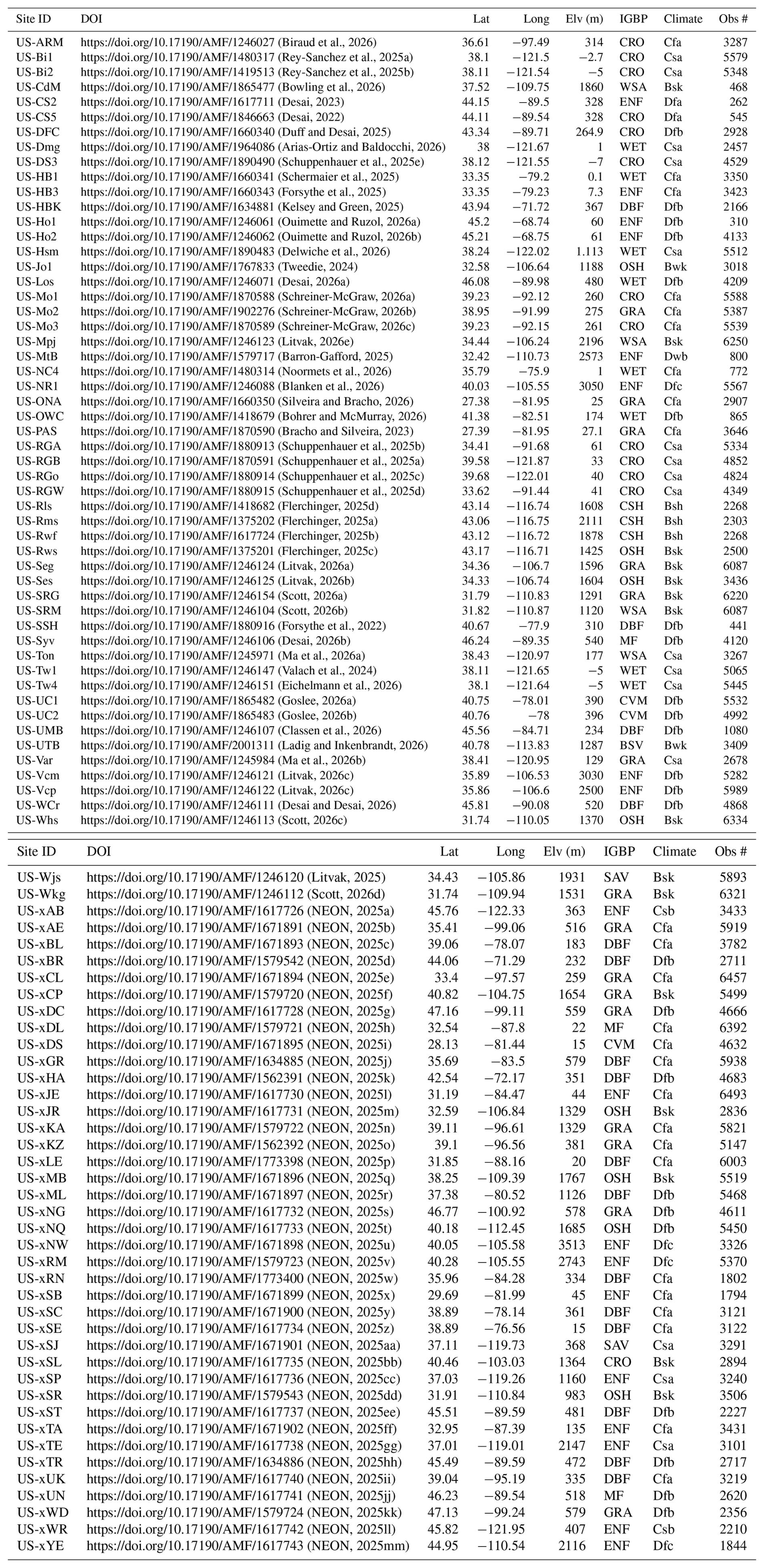
Table A2 International Geosphere-Biosphere Programme (IGBP) Land Cover Classes and Köppen Climate Classes and their abbreviations as well as the number of sites in each category (abbreviations, # of sites).

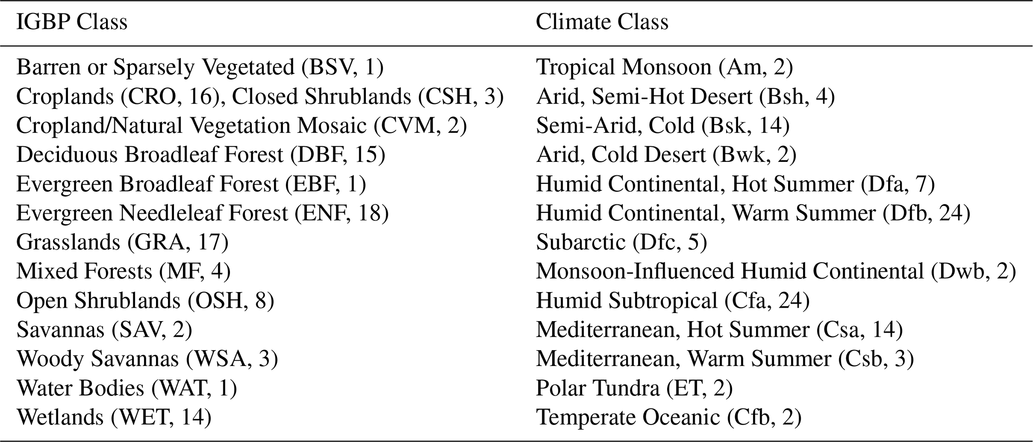
Table A3 Performance of ALIVE_ET under clear and cloudy sky conditions using optimal models (GBR for daytime, LSTM for nighttime).

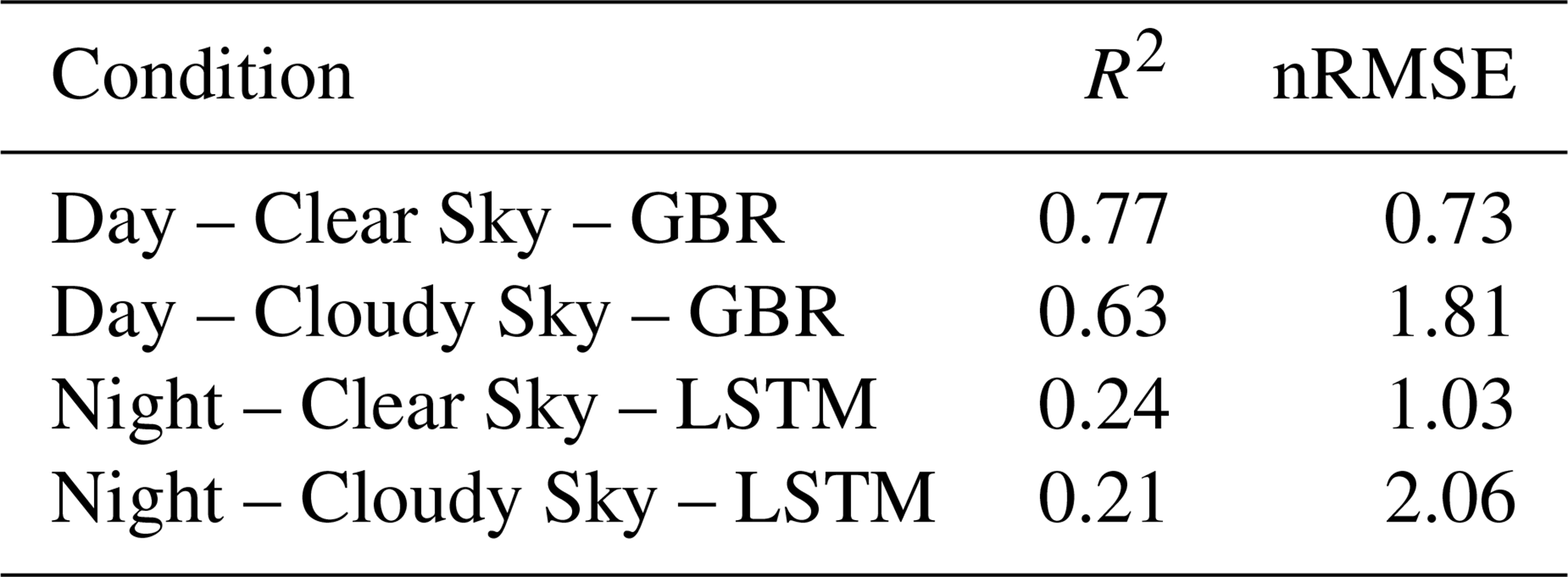
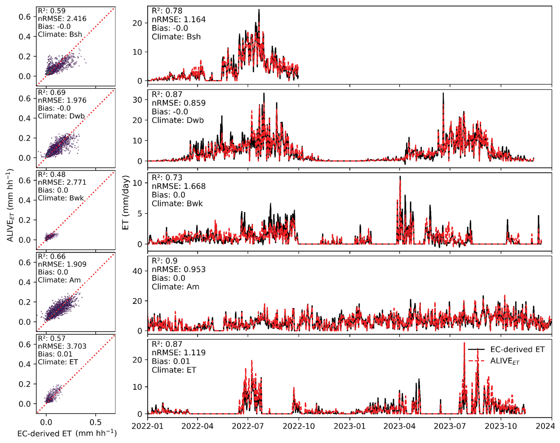
Figure A1 ALIVE_ET estimates compared to EC-derived ET across different Köppen climate classes. Left panels display density scatter plots of half-hourly estimates, while right panels show daily time series of ALIVE_ET vs. EC-derived ET for 2022 and 2023.

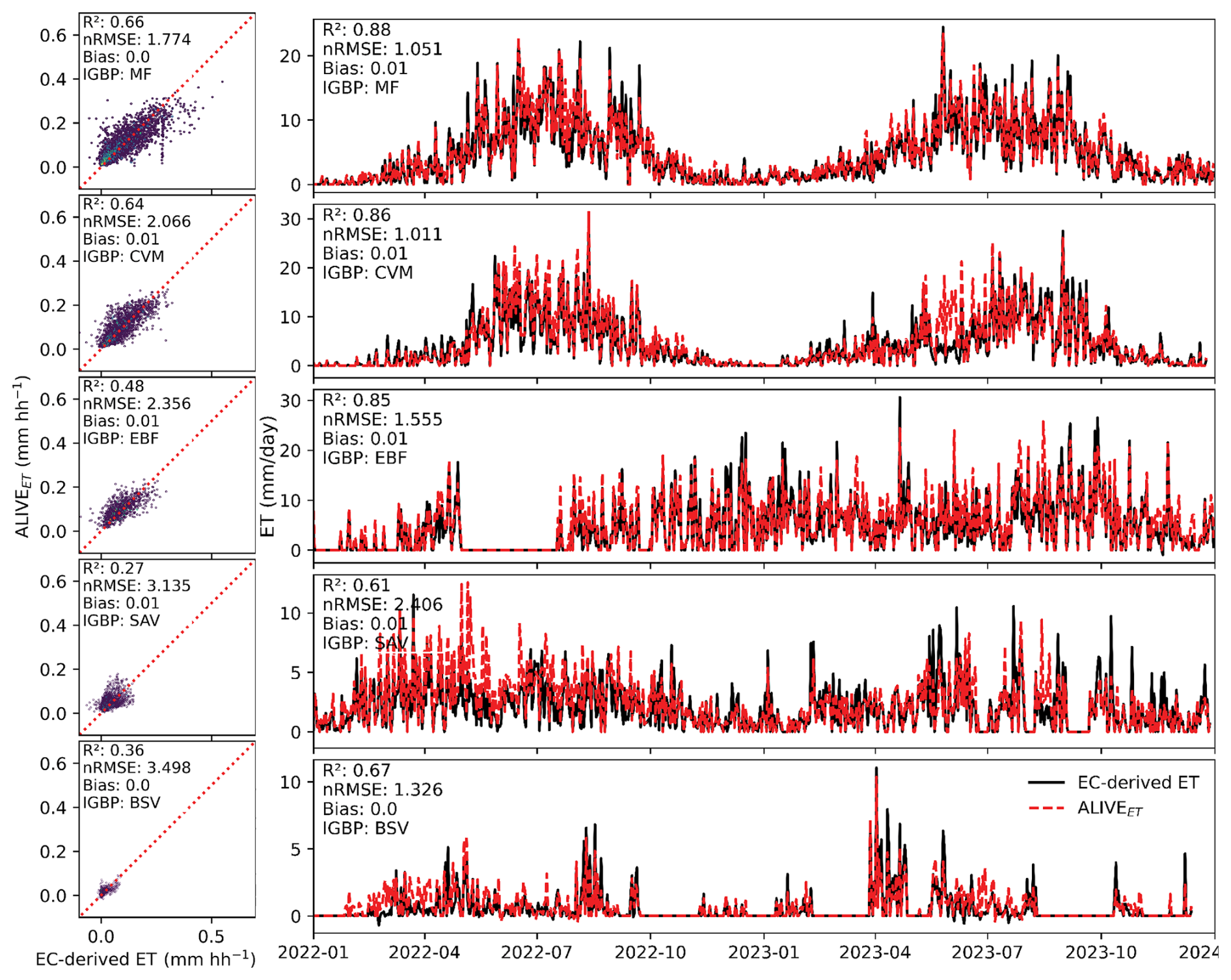
Figure A2 Comparison of ALIVE_ET estimates with EC-derived ET across different IGBP land cover types. Left panels show density scatter plots of half-hourly estimates, while right panels display daily time series of ALIVE_ET vs. EC-derived ET for 2022 and 2023.