A non-stationary trans-Gaussian model for daily rainfall over complex topography

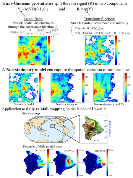
In mountainous regions orographic effects create strong horizontal gradients of various rainfall statistics such as the frequency of occurrence, the distribution of intensity and the structure of spatial correlation. However, most statistical models of daily rainfall assume spatial stationarity (i.e., the spatial homogeneity of rainfall statistics) and are therefore not well suited for studying the highly non-homogeneous characteristics of orographic rainfall. To overcome this limitation, we design a non-stationary trans-Gaussian geostatistical model for the analysis of daily rainfall fields over complex topography. This framework infers rainfall statistics from sparse rain gauge observations, simulates realistic rainfall fields after calibration and stochastically interpolates rain gauge observations to create rainfall maps. The performance of the model is assessed with data from the Island of Hawai`i where extreme spatial gradients in rainfall are observed. Results demonstrate that the non-stationary trans-Gaussian model can skillfully reproduce orographic rainfall statistics as well as their variations in space.

1 Introduction

Stochastic rainfall models (SRMs) are probabilistic tools that simulate synthetic rainfall datasets with statistical properties that resemble those from observations (Richardson, 1981; Wilks and Wilby, 1999; Sharma and Mehrotra, 2010; Ailliot et al., 2015). These models first infer the probability distribution of rainfall from observations and then generate synthetic datasets by random sampling of this distribution, a process known as stochastic simulation. Stochastic simulation makes SRMs particularly suitable to assess the uncertainty of rainfall estimates (Vischel et al., 2009; Caseri et al., 2016) and forecasts (Bowler et al., 2006; Nerini et al., 2017), and to assess the natural variability of rainfall (Evin et al., 2018; Peleg et al., 2018). The ability of SRMs to simulate probabilistic ensembles of synthetic but realistic rainfall data makes them an important tool for rainfall-related impact studies, for instance to perform dam or drainage system sizing (Niemi et al., 2016), hydro-meteorological modeling (Mandapaka et al., 2009; Paschalis et al., 2014), or crop yield simulation (Hansen and Ines, 2005; Qian et al., 2011).

A large variety of stochastic models have been applied to rainfall modeling, the choice of which depends on the features of rainfall to reproduce in priority. For instance, point process models have been used to simulate the occurrence of the main meteorological processes responsible for rainfall generation (e.g., rain cells, rain bands, storms) (Onof et al., 2000; Cowpertwait, 2010), models combining Markov chains and parametric distributions of rain intensity (Richardson, 1981; Ailliot et al., 2009) as well as resampling approaches (Rajagopalan and Lall, 1999; Oriani et al., 2014) have been applied to time-series simulation, generalized linear models have been used to capture the relationships between atmospheric conditions and rainfall (Chandler and Wheater, 2002; Chandler, 2020), fractal approaches have shown good performance in simulating rainfall scaling properties (Molnar and Burlando, 2005; Ramanathan et al., 2022; Maloku et al., 2025), and generative AI recently demonstrated promising skills at downscaling and forecasting complex rainfall features (Leinonen et al., 2020; Ravuri et al., 2021; Harris et al., 2022; Srivastava et al., 2024).

When the focus is on spatial patterns and spatial dependencies, models based on Gaussian random fields (GRFs) – also known as geostatistical models – are often chosen because they enable modeling rainfall at any point of the spatial domain while accounting for spatial dependencies (Chilès and Delfiner, 2012). However, the distribution of rainfall intensity is rarely Gaussian at daily to sub-daily resolution, and a parametric transform function is often combined with a GRF to model rainfall at these time scales resulting in so-called trans-Gaussian (or meta-Gaussian) approaches (Leblois and Creutin, 2013; Benoit et al., 2018; Papalexiou and Serinaldi, 2020). Trans-Gaussian models can be used to simulate rainfall in two main settings: unconditional simulations allow for the generation of synthetic rainfall fields (Paschalis et al., 2013; Peleg et al., 2017; Vaittinada Ayar et al., 2020; Wilcox et al., 2021) while conditional simulations are used for mapping rainfall from sparse rain gauge observations (Creutin and Obled, 1982; Lanza, 2000; Kyriakidis et al., 2001) and for radar-rain gauge data fusion (Creutin et al., 1988; Foehn et al., 2018). In both cases the resulting rainfall datasets can be used to assess input errors in distributed hydrological models (Vischel et al., 2009; Renard et al., 2011) or to conduct sensitivity analysis of spatially explicit hydro-meteorological modeling chains (Moraga et al., 2022; Liu et al., 2024).

In mountainous regions, the performance of trans-Gaussian models is constrained by the strong variability of rainfall statistics through space. Indeed, air masses flowing across mountains are displaced by the topography and forced into successive uplifts and downdrafts. The vertical displacement of air modulates the condensation within the air column, triggering or enhancing precipitation in the case of uplift and, conversely, inhibiting or attenuating rainfall in the case of downdraft. This impact of topography on precipitation is called the orographic effect (Roe, 2005; Houze, 2012) and results in windward slopes being generally wetter than leeward slopes and the highlands generally wetter than the lowlands (Foresti et al., 2018). Additionally, fluctuations in the direction and intensity of prevailing winds combined with changes of precipitation regimes lead to complex patterns of orographic rainfall with strong spatial gradients between wet and dry areas (Giambelluca et al., 2013; Isotta et al., 2014; Benoit and Sichoix, 2023).

In this context, the present study intends to develop a trans-Gaussian model for daily rainfall over complex topography, which requires to adapt the trans-Gaussian framework to the spatial variation of rainfall statistics caused by orographic effects. This implies making some parameters of the model location-dependent, a condition referred to as spatial non-stationarity (Sampson and Guttorp, 1992). Two approaches have been proposed so far to make trans-Gaussian rainfall models non-stationary: either the marginal distribution (i.e., the parameters modeling rainfall occurrence and intensity) is made non-stationary (Frazier et al., 2016; Benoit et al., 2021; Lucas et al., 2022), or the non-stationarity is modeled in the covariance function (i.e., the parameters modeling the spatial dependencies within rainfall fields) (Paciorek and Schervish, 2006; Fuglstad et al., 2015; Fouedjio et al., 2016). In this paper we aim to combine these two ways of modeling spatial non-stationarity, which leads to what we call a fully non-stationary trans-Gaussian model, i.e., a trans-Gaussian model with all parameters varying in space. This provides a very flexible spatial model for daily rainfall, in which the statistics characterizing (1) rainfall occurrence, (2) the marginal distribution of rainfall intensity and (3) the spatial dependencies within rainfall fields are location-dependent. The performance of the model is illustrated for the Island of Hawai`i (State of Hawaii, USA) where orographic effects are very strong (Giambelluca et al., 2013), and for which an extensive and high-quality rain gauge dataset enables the calibration of a highly parametrized model. The model is designed and tested with two specific applications in mind: the interpolation of rain gauge data to generate daily rainfall maps for the Hawai`i Climate Data Portal (HCDP) (Longman et al., 2024), and the stochastic generation of spatially explicit rainfall fields to foster hydrological modeling in Hawai`i (Huang et al., 2021; Strauch et al., 2024).

The rest of the paper is structured as follows: Sect. 2 illustrates orographic precipitation on the Island of Hawai`i and motivates the need for a non-stationary rainfall model. Section 3 describes the trans-Gaussian model being used, explains how to make it non-stationary in space and proposes a method for model calibration. Section 4 applies the model to the simulation of orographic rainfall on the Island of Hawai`i and assesses the performance of the model. Finally, Sect. 5 discusses the advantages and limitations of the model with respect to orographic rainfall modeling and proposes some lines of inquiry for future research.

2 Example dataset: orographic precipitation on the Island of Hawai`i

Due to the location of the Island of Hawai`i (State of Hawaii – USA, area = 10 432 km<sup>2</sup>, highest point: Mauna Kea – 4207 m) in the middle of the subtropical Pacific (Fig 1a), the climate of the island is shaped by prevailing easterly trade winds which blow 85 %–95 % of the time in summer and 50 %–80 % of the time in winter (Longman et al., 2021). When they reach the Island of Hawai`i, trade winds produce the orographic lifting of moist oceanic air masses, which triggers shallow convection leading to frequent and abundant rain showers in the east facing slopes and generally dry conditions on the leeward west side of the island (Fig 1b) (Giambelluca et al., 2013). An exception to these generally dry weather conditions is a distinct rainfall maximum in the Kona area (West from Mauna Loa, at around 5 km from the coast) which is the result of mechanically diverted tradewinds being directed upslope, enhanced in the afternoon by strong solar heating of the west-facing slope (Huang and Chen, 2019).

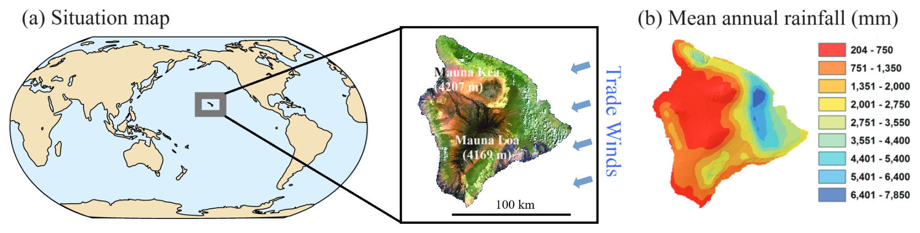
Figure 1 Geographical and climatological context of the Island of Hawai`i. (a) Situation map and main topo-climatic features (adapted from an ETM+ Landsat 7 mosaic produced by NOAA Coastal Services Center as part of the Hawaii Land Cover Analysis project), (b) mean annual rainfall (adapted from Giambelluca et al. (2013)).

In Hawai`i weather conditions are often affected by the presence of the trade wind inversion (TWI, average inversion base height around 2200 m) that caps the moist oceanic air and creates very dry conditions at high altitudes located in the center of the island (Fig 1b) (Longman et al., 2015). This predominant pattern of precipitation is drastically modified when atmospheric disturbances originating from the mid-latitudes (e.g., cold fronts or Kona lows) eliminate the TWI, produce southerly, southwesterly, or westerly winds at the regional scale, and allow deep convection to develop. Under atmospheric disturbance conditions, widespread rainfall occurs throughout the island, and the west-facing slopes as well as the high altitude locations, which are usually dry, receive a significant part of their annual precipitation (Longman et al., 2021).

To account for the diversity of climate patterns in the State of Hawaii, Luo et al. (2024) proposed a partitioning of the archipelago into twelve climate divisions (Fig 2). Climate divisions constitute the basic geographic unit used by the National Oceanic and Atmospheric Administration's National Centers for Environmental Information (NCEI-NOAA) for climate analyses at the scale of the United States of America (Guttman and Quayle, 2005). The Hawai`i climate divisions have been defined based on a cluster analysis on monthly rainfall maps and local expert knowledge (Luo et al., 2024), and will be used in the present study to delineate six sub-domains of the island of Hawai`i within which the rainfall climatology is assumed to be relatively homogeneous (Fig. 2a).

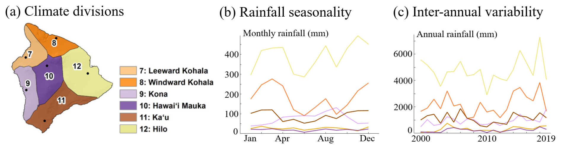
Figure 2 Climate divisions of the Island of Hawai`i. (a) Footprint of the climate divisions (adapted from Luo et al. (2024); the numbering over the Island of Hawai`i starts at 7 because the original zonation covers the whole State of Hawaii). (b) Rainfall seasonality and (c) rainfall inter-annual variability for 6 rain gauges spread in the different climate divisions (gauge locations are denoted by black dots in a).

Figures 1b and 2b–c illustrate the diversity of rainfall climatology over the Island of Hawai`i. This diversity translates into a strong heterogeneity of rainfall statistics throughout the island, which calls for a non-stationary trans-Gaussian model for the spatial analysis of daily rainfall. Such a model is introduced in the next section and applied to the Island of Hawai`i in Sect. 4.

3 Non-stationary trans-Gaussian rainfall model

In the following, we model daily rainfall as a stochastic process studied over a spatial domain 𝒟: R(s) with $\mathit{s}\in \mathcal{D}\subset {\mathbb{R}}^{\mathrm{2}}$. As the focus of the study is on the spatial modeling of rainfall, we model the temporal variability separately (and beforehand) following a rain-typing approach (Ailliot et al., 2015; Blanchet et al., 2019; Vaittinada Ayar et al., 2020). We therefore assume that days can preliminarily be pooled into N_clust clusters referred to hereafter as rain types, within which rainfall fields are statistically similar to each other. All the information about the temporal variability of rainfall is therefore encoded into the sequence of rain types, which has been shown to be a reasonable assumption for daily rainfall in tropical islands, and in particular in Hawai`i (Benoit et al., 2022). As a result, daily rainfall fields are assumed independent to each other conditionally to rain types. The spatial modeling is therefore performed independently for each rain type, and for the sake of simplicity we assume a single rain type for the description of the model in Sect. 3.1 to 3.5. How to deal with multiple rain types when conditioning daily rainfall maps to monthly totals will be addressed in Sect. 3.6, and the practical delineation of rain types from an actual dataset will be addressed in Sect. 4.1.

3.1 Trans-Gaussian geostatistics applied to rainfall modeling

When observed at a single site and at daily resolution, rainfall is featured by a large number of zeros (i.e. dry days) and a distribution of non-zero rainfall intensities that strongly differs from the normal distribution (Evin et al., 2018; Blanchet et al., 2019; Benoit et al., 2022). In addition, when observed simultaneously at neighboring locations, rainfall is structured spatially with inter-site dependencies decreasing with the separation distance and vanishing at distances of dozens to hundreds of kilometers depending on the regional climate (Creutin et al., 1988; Guillot and Lebel, 1999). In this study we adopt a trans-Gaussian approach to model the above features of rainfall (Allard and Bourotte, 2015; Benoit et al., 2018; Papalexiou and Serinaldi, 2020; Vaittinada Ayar et al., 2020). Trans-Gaussian geostatistics assume that a rainfall observation R(s) performed at location s∈𝒟 originates from a latent and standardized (i.e., with zero mean and unit variance) Gaussian random variable Y(s) through a transform function Ψ which combines a truncation at threshold a₀ and a monotonic transformation ψ of the non-censored part of the latent variable. The spatial dependencies observed between a set of N rain observations performed at different locations $R\left({\mathit{s}}_i\right),i=\mathrm{1},\mathrm{\dots },N_G$ are modeled by assuming that the associated latent variables $Y\left({\mathit{s}}_i\right),i=\mathrm{1},\mathrm{\dots },N_G$ form a random vector $\mathit{Y}=\left[Y\right({\mathit{s}}_{\mathrm{1}}),Y({\mathit{s}}_{\mathrm{2}}),\mathrm{\dots },Y({\mathit{s}}_{N_G}\left)\right]$ that follows a standardized multivariate Gaussian distribution with covariance function C_Y.

In the following of Sect. 3.1 and in Sect. 3.2 we develop a Trans-Gaussian rainfall model tailored to the example dataset introduced in Sect. 2, which entails choosing parameterizations of ψ and C_Y that best fit the statistical signature of rainfall in the Island of Hawai`i. A different dataset, in particular from a different climate, could require different parameterizations of these functions without calling into question the non-stationary Trans-Gaussian framework deployed in this study.

Here we assume a Gamma distribution for single-site rain intensity (Wilks and Wilby, 1999; Berrocal et al., 2008) because this distribution has easy-to-interpolate parameters (i.e., with high auto-correlation and low cross-correlation) and because when combined with rain types the Gamma distribution has been shown to accurately model daily rainfall intensity (Blanchet et al., 2019). In addition we assume a Matérn covariance function for the latent Gaussian random field because this model of covariance is very flexible (Porcu et al., 2024) and has shown good skills in modeling the spatial dependencies of most atmospheric variables, including rainfall, at daily resolution (Obakrim et al., 2025). Finally, a geometric anisotropy is added to the model of covariance to allow spatial dependencies to vary with the direction of interest (Allard et al., 2016). Overall, the trans-Gaussian model for daily rainfall is defined as:

$$\begin{array}{}\text{(1)}& \begin{array}{rl}R\left(\mathit{s}\right)& =\mathrm{\Psi }\left(Y\right(\mathit{s}\left)\right)\\ & =\left\{\begin{array}{l}\mathrm{0}\mathrm{if}Y\left(\mathit{s}\right)\le a_{\mathrm{0}}\\ {\mathrm{Gamma}}^{-\mathrm{1}}\left(\mathrm{\Phi }\right(Y\left(\mathit{s}\right));k,\mathit{\theta })\mathrm{if}Y\left(\mathit{s}\right)>a_{\mathrm{0}}\end{array}\right.\end{array}\end{array}$$

With $Y\sim \mathcal{N}\left(\mathrm{0},C_Y\right)$ and $C_Y(\mathit{h};\mathit{\nu },{\mathit{\gamma }}_{a,\mathrm{1}},{\mathit{\gamma }}_{a,\mathrm{2}},{\mathit{\rho }}_b)=\frac{\mathrm{1}}{\mathrm{\Gamma }\left(\mathit{\nu }\right){\mathrm{2}}^{\mathit{\nu }-\mathrm{1}}}{\left(\sqrt{Q}\right)}^{\mathit{\nu }}{\mathcal{K}}_{\mathit{\nu }}\left(\sqrt{Q}\right)$ and with $Q={\mathit{h}}^T\times \mathbf{\Sigma }\times \mathit{h}$; $\mathbf{\Sigma }=\mathit{V}\times \mathbf{\Lambda }\times {\mathit{V}}^T$; $\mathit{V}=\left[\begin{array}{cc}\frac{{\mathit{\gamma }}_{a,\mathrm{1}}}{\sqrt{{\mathit{\gamma }}_{a,\mathrm{1}}^{\mathrm{2}}+{\mathit{\gamma }}_{a,\mathrm{2}}^{\mathrm{2}}}}& -\frac{{\mathit{\gamma }}_{a,\mathrm{2}}}{\sqrt{{\mathit{\gamma }}_{a,\mathrm{1}}^{\mathrm{2}}+{\mathit{\gamma }}_{a,\mathrm{2}}^{\mathrm{2}}}}\\ \frac{{\mathit{\gamma }}_{a,\mathrm{2}}}{\sqrt{{\mathit{\gamma }}_{a,\mathrm{1}}^{\mathrm{2}}+{\mathit{\gamma }}_{a,\mathrm{2}}^{\mathrm{2}}}}& \frac{{\mathit{\gamma }}_{a,\mathrm{1}}}{\sqrt{{\mathit{\gamma }}_{a,\mathrm{1}}^{\mathrm{2}}+{\mathit{\gamma }}_{a,\mathrm{2}}^{\mathrm{2}}}}\end{array}\right]$;
$\mathbf{\Lambda }=\left[\begin{array}{cc}{\mathit{\gamma }}_{a,\mathrm{1}}^{\mathrm{2}}+{\mathit{\gamma }}_{a,\mathrm{2}}^{\mathrm{2}}& \mathrm{0}\\ \mathrm{0}& {\mathit{\rho }}_b^{\mathrm{2}}\end{array}\right]$ where $\mathrm{Gamma}(\cdot ;k,\mathit{\theta })$ is the cumulative distribution function (cdf) of the Gamma distribution with parameters k>0 (shape) and θ>0 (scale); Φ is the cdf of the standardized normal distribution; h is the separation vector between two locations s_i and s_j; Γ is the usual gamma function; 𝒦_ν is the modified Bessel function of the second kind with parameter ν>0, and ν is the shape parameter of the Matérn covariance function that controls the regularity of the latent process Y at short separation lags; ${\mathit{\gamma }}_{a,\mathrm{1}}\in \mathbb{R}$ and ${\mathit{\gamma }}_{a,\mathrm{2}}\in \mathbb{R}$ are the two components of the vector defining the major anisotropy axis (whose direction corresponds to the direction of maximum spatial correlation of the latent process Y and whose norm ${\mathit{\rho }}_a=\sqrt{{\mathit{\gamma }}_{a,\mathrm{1}}^{\mathrm{2}}+{\mathit{\gamma }}_{a,\mathrm{1}}^{\mathrm{2}}}$ controls the variability of Y in that direction); and ρ_b>0 is the norm of the minor anisotropy axis vector (which is orthogonal to the major anisotropy axis vector).

3.2 Making the trans-Gaussian model non-stationary

The trans-Gaussian model of Eq. (1) is made fully non-stationary in space by allowing the parameters of the marginal distribution and those of the dependence structure to vary through space. To this end, the parameters of the transform function Ψ (i.e., a₀, k and θ) are first defined for each observation location separately, and then interpolated at ungauged locations (Blanchet et al., 2019; Benoit et al., 2021; Maloku et al., 2025). Making the parameters of the covariance function C_Y (i.e., ν, γ_a,1, γ_a,2, and ρ_b) non-stationary is more challenging because the resulting covariance function must be a valid model of covariance over the whole domain of interest (Chilès and Delfiner, 2012). Different approaches have been proposed to obtain valid non-stationary covariance models, for instance the convolution of locally stationary covariance kernels (Paciorek and Schervish, 2006; Fouedjio et al., 2016), the space deformation of the modeling domain (Sampson and Guttorp, 1992; Fouedjio et al., 2015), and the use of a locally varying diffusion operator in stochastic partial differential equations (Fuglstad et al., 2015; Pereira et al., 2022). Here we follow the convolution approach because it provides a direct extension of the Matérn covariance function defined in Eq. (1) to the non-stationary case, and because the use of locally stationary covariance kernels simplifies the calibration of the model based on sparse rain gauge observations (cf. Sect. 3.3). We adopt the parametrization of Paciorek and Schervish (2006) to derive the non-stationary and anisotropic covariance function of Matérn type between two observation locations s_i and s_j:

$$\begin{array}{}\text{(2)}& \begin{array}{rl}{C}_Y& ({\mathit{s}}_i,{\mathit{s}}_j;{\mathit{\nu }}_i,{\mathit{\nu }}_j,{{\mathit{\gamma }}_{a,\mathrm{1}}}_i,{{\mathit{\gamma }}_{a,\mathrm{1}}}_j,{{\mathit{\gamma }}_{a,\mathrm{2}}}_i,{{\mathit{\gamma }}_{a,\mathrm{2}}}_j,{{\mathit{\rho }}_b}_i,{{\mathit{\rho }}_b}_j)\\ & ={\displaystyle \frac{{\mathrm{2}}^{\mathrm{1}-{\mathit{\nu }}_{ij}}}{\sqrt{\mathrm{\Gamma }\left({\mathit{\nu }}_i\right)\mathrm{\Gamma }\left({\mathit{\nu }}_j\right)}}}{\left|{\mathbf{\Sigma }}_i\right|}^{\frac{\mathrm{1}}{\mathrm{4}}}{\left|{\mathbf{\Sigma }}_j\right|}^{\frac{\mathrm{1}}{\mathrm{4}}}{\left|{\displaystyle \frac{{\mathbf{\Sigma }}_i+{\mathbf{\Sigma }}_j}{\mathrm{2}}}\right|}^{-\frac{\mathrm{1}}{\mathrm{2}}}{\left(\sqrt{Q_{ij}}\right)}^{{\mathit{\nu }}_{ij}}{\mathcal{K}}_{{\mathit{\nu }}_{ij}}\left(\sqrt{Q_{ij}}\right)\end{array}\end{array}$$

with $Q_{ij}={\left({\mathit{s}}_i-{\mathit{s}}_j\right)}^T{\left(\frac{{\mathbf{\Sigma }}_i+{\mathbf{\Sigma }}_j}{\mathrm{2}}\right)}^{-\mathrm{1}}\left({\mathit{s}}_i-{\mathit{s}}_j\right)$, with ${\mathit{\nu }}_{ij}=\frac{{\mathit{\nu }}_i+{\mathit{\nu }}_j}{\mathrm{2}}$ and with Σ_i and Σ_j defined as in Eq. (1).

3.3 Model calibration

Model calibration starts with the estimation of model parameters at the local scale assuming local stationarity, and continues with the interpolation of these parameters to create a non-stationary model. The data used for calibration are daily rainfall measurements performed by a rain gauge network encompassing a set 𝒩_etwork of N_g observation locations s_g positioned within the study domain 𝒟: ${\mathit{s}}_{\mathrm{g}}\in {\mathcal{N}}_{\mathrm{etwork}}\subset \mathcal{D},$ $g=\mathrm{1},\mathrm{\dots },N_g$.

3.3.1 Estimation of model parameters assuming local stationarity

The basic unit for the estimation of locally stationary parameters of the transform function is the rain gauge. Hence, for a given rain gauge at location s_g, the truncation threshold a₀(s_g) is obtained from the proportion d(s_g) of dry measurements observed at this location by simply inverting the cdf of a standardized normal distribution $a_{\mathrm{0}}\left({\mathit{s}}_{\mathrm{g}}\right)={\mathrm{\Phi }}^{-\mathrm{1}}\left(d\right({\mathit{s}}_{\mathrm{g}}\left)\right)$, and then the parameters of the marginal distribution of non-zero daily intensities (i.e. k and θ) are estimated by marginal likelihood maximization. The log-likelihood of the parameters k and θ given a set of N_obs non-zero rain observations performed at location s_g (i.e., R_j(s_g)>0, $j=\mathrm{1},\mathrm{\dots },N_{\mathrm{obs}}$) is:

$$\begin{array}{}\text{(3)}& l(k,\mathit{\theta })=\sum _{j=\mathrm{1}}^{N_{\mathrm{obs}}}\left(\ln \left({\displaystyle \frac{\mathrm{1}}{\mathrm{\Gamma }\left(k\right){\mathit{\theta }}^k}}{R}_j({\mathit{s}}_{\mathrm{g}}{)}^{k-\mathrm{1}}{e}^{-\frac{R_j\left({\mathit{s}}_{\mathrm{g}}\right)}{\mathit{\theta }}}\right)\right)\end{array}$$

The estimation of covariance parameters requires observations from several rain gauges simultaneously to capture spatial dependence, and therefore the basic unit used for the estimation of locally stationary parameters of the covariance function is the climate division. Climate divisions form sub-domains of the target area within which the climatology of rainfall is deemed relatively homogeneous (cf. Sect. 2), which allows us to make an assumption of local stationarity for the dependence structure. The size of the climate divisions used as sub-domains where local stationarity is postulated derives from the tradeoff between (i) the number of rain gauges within each division that should be maximized to improve the estimation of the covariance parameters and (ii) the distance between climate divisions that should be minimized to improve the performance of the interpolation used to build the non-stationary covariance model. After the delineation of climate divisions, the parameters of the covariance function C_Y of the latent field are estimated for each division separately using pairwise likelihood maximization, which has been proved to be an efficient and unbiased method for the estimation of covariance parameters (Bevilacqua et al., 2012). For a given pair of rain observations $R\left({\mathit{s}}_{g_{\mathrm{1}}}\right)$ and $R\left({\mathit{s}}_{g_{\mathrm{2}}}\right)$ recorded the same day by two rain gauges at locations ${\mathit{s}}_{g_{\mathrm{1}}}\in {\mathcal{N}}_{\mathrm{etwork}}$ and ${\mathit{s}}_{g_{\mathrm{2}}}\in {\mathcal{N}}_{\mathrm{etwork}}$ with separation vector $\mathit{h}={\mathit{s}}_{g_{\mathrm{2}}}-{\mathit{s}}_{g_{\mathrm{1}}}$ the log-likelihood of the parameters ν, γ_a,1, γ_a,2 and ρ_b can be written as (Allard and Bourotte, 2015):

$$\begin{array}{}\text{(4)}& \begin{array}{rl}l& (\mathit{\nu },{\mathit{\gamma }}_{a,\mathrm{1}},{\mathit{\gamma }}_{a,\mathrm{2}},{\mathit{\rho }}_b)=\ln \left({\mathrm{\Phi }}_{\mathrm{2}}\right(a_{\mathrm{0}},a_{\mathrm{0}};C_Y(\mathit{h};\mathit{\nu },{\mathit{\gamma }}_{a,\mathrm{1}},{\mathit{\gamma }}_{a,\mathrm{2}},{\mathit{\rho }}_b)\left)\right)\\ & \mathrm{if}R\left({\mathit{s}}_{g_{\mathrm{1}}}\right)=R\left({\mathit{s}}_{g_{\mathrm{2}}}\right)=\mathrm{0}\\ & l(\mathit{\nu },{\mathit{\gamma }}_{a,\mathrm{1}},{\mathit{\gamma }}_{a,\mathrm{2}},{\mathit{\rho }}_b)=\ln \left(\mathrm{\Phi }\right(a_{\mathrm{0}})-{\mathrm{\Phi }}_{\mathrm{2}}(a_{\mathrm{0}},a_{\mathrm{0}};C_Y(\mathit{h};\mathit{\nu },{\mathit{\gamma }}_{a,\mathrm{1}},{\mathit{\gamma }}_{a,\mathrm{2}},{\mathit{\rho }}_b)\left)\right)\\ & +\ln \left(\mathit{\varphi }\right(Y\left({\mathit{s}}_{g_{\mathrm{2}}}\right)\left)\right)\\ & \mathrm{if}R\left({\mathit{s}}_{g_{\mathrm{1}}}\right)=\mathrm{0}\mathrm{and}R\left({\mathit{s}}_{g_{\mathrm{2}}}\right)>\mathrm{0}\\ & l(\mathit{\nu },{\mathit{\gamma }}_{a,\mathrm{1}},{\mathit{\gamma }}_{a,\mathrm{2}},{\mathit{\rho }}_b)=\ln \left({\mathit{\varphi }}_{\mathrm{2}}\right(Y\left({\mathit{s}}_{g_{\mathrm{1}}}\right),Y\left({\mathit{s}}_{g_{\mathrm{2}}}\right);C_Y(\mathit{h};\mathit{\nu },{\mathit{\gamma }}_{a,\mathrm{1}},{\mathit{\gamma }}_{a,\mathrm{2}},{\mathit{\rho }}_b)\left)\right)\\ & \mathrm{if}R\left({\mathit{s}}_{g_{\mathrm{1}}}\right)>\mathrm{0}\mathrm{and}R\left({\mathit{s}}_{g_{\mathrm{2}}}\right)>\mathrm{0}\end{array}\end{array}$$

where Φ₂ and ϕ₂ are respectively the cdf and the probability density function (pdf) of the bivariate standard normal distribution, ϕ is the pdf of the univariate standard normal distribution, and $Y\left({\mathit{s}}_{g_{\mathrm{1}}}\right)$ is the latent counterpart of the rainfall observation $R\left({\mathit{s}}_{g_{\mathrm{1}}}\right)$.

The log-likelihoods of the marginal distribution and covariance function are maximized sequentially using the fmincon function in Matlab (using the default interior point algorithm (Byrd et al., 1999)). This sequential estimation scheme has shown good performance in estimating the parameters of trans-Gaussian models of rainfall (Leblois and Creutin, 2013; Caseri et al., 2016; Papalexiou and Serinaldi, 2020).

3.3.2 Spatial interpolation of model parameters

Once the parameters of the model are known locally for each rain gauge and climate division, they can be propagated to the entire domain of interest by spatial interpolation.

To interpolate the parameters of the transform function Ψ we use ordinary Kriging with a nugget term and a Matérn covariance function (Bennett et al., 2018) applied directly to the parameters inferred at rain gauge locations. To interpolate the parameters of the covariance function C_Y we assign the locally stationary values to the barycenter of each climate division, and then interpolate them through space using a squared inverse distance interpolation because in the targeted application the small number of climate divisions does not allow for more complex interpolation techniques such as Kriging (Babak and Deutsch, 2009).

After interpolation, all parameters of the trans-Gaussian model are known at every point of the study domain 𝒟. The parameters of the transform function Ψ can be used to transform rainfall values to their latent counterpart (and vice versa), and the parameters of the covariance function C_Y can be used to build a model of non-stationary covariance as defined in Eq. (2).

3.4 Simulating synthetic rainfall fields by stochastic simulation

Synthetic rainfall fields reproducing the statistics of the training dataset are generated by stochastic simulation performed at a set of N_T target locations u_i often located on a regular lattice grid to comply with the requirement of impact models: ${\mathit{u}}_i\in \mathcal{G}\mathit{rid}\subset \mathcal{D},i=\mathrm{1},\mathrm{\dots },N_{\mathrm{T}}$. Note that target locations are denoted by u_i to distinguish them from rain gauge locations s_g, and we recall here that model parameters at target locations derive from the spatial interpolation of the parameter values estimated at gauge locations.

To simulate synthetic rainfall fields, a realization of the latent field is first generated by geostatistical simulation. A simple way to draw this realization is by Cholesky decomposition of the covariance matrix C_Y (Davis, 1987):

$$\begin{array}{}\text{(5)}& {\mathit{Y}}_{\mathrm{us}}=\mathbf{L}\times {\mathit{V}}_{\mathrm{iid}}\end{array}$$

where Y_us is the vector containing the realization of the latent field Y_us at target locations u_i, L is the lower triangular matrix resulting from the Choleski decomposition of the covariance matrix C_Y evaluated at the target locations (i.e., $C_Y=\mathbf{L}\times {\mathbf{L}}^{\mathrm{T}}$) and V_iid is an independent and identically distributed standardized normal vector of size N_T.

Standard algorithms for the Cholesky decomposition of the covariance matrix have a complexity of $\mathcal{O}\left(N{{}_T}^{\mathrm{3}}\right)$ point operations and a memory footprint of $\mathcal{O}\left(N{{}_T}^{\mathrm{2}}\right)$ (Abdulah et al., 2019), which can be prohibitive when more than a few thousands of simulation points are intended. When more target points are requested the simulation based on the Cholesky decomposition of the covariance matrix can be replaced by an approximate but more scalable simulation method, for instance based on a spectral approach that scales linearly with the number of simulation points (Emery and Arroyo, 2018; Allard et al., 2025).

A synthetic rainfall field is finally obtained by transformation of the latent field:

$$\begin{array}{}\text{(6)}& R_{\mathrm{us}}\left({\mathit{u}}_i\right)={\mathrm{\Psi }}_{{\mathit{u}}_i}\left(Y_{\mathrm{us}}\right({\mathit{u}}_i\left)\right)\end{array}$$

where Y_us(u_i) is the realization of latent field at target location u_i and ${\mathrm{\Psi }}_{{\mathit{u}}_i}$ is the local transform function at the same location. Note that an ensemble of N_sim realizations (i.e., $R_{\mathrm{us}}^k\left({\mathit{u}}_i\right)$, $i=\mathrm{1},\mathrm{\dots },N_{\mathrm{T}}$, $k=\mathrm{1},\mathrm{\dots },N_{\mathrm{sim}}$) can be obtained by iterating N_sim times the Eqs. (5) and (6) with different realizations of the vector V_iid.

3.5 Rainfall mapping by stochastic interpolation of daily rain gauge observations

Rainfall maps and associated uncertainty estimations can be obtained by the stochastic interpolation of the rain gauge observations. To this end, the ensemble of synthetic rainfall fields $R_{\mathrm{us}}^k$ described above is modified by a process called conditioning that forces them to reproduce rain gauge observations. An efficient way to perform conditioning in the framework of Geostatistics is conditioning by Kriging (Chilès and Delfiner, 2012). Since conditioning by Kriging requires a target variable with a multivariate Gaussian distribution, it should be performed on the latent field $Y_{\mathrm{us}}^k$. Hence, conditioning a synthetic rainfall field requires the computation of the latent counterparts of rainfall observations $Y\left(\mathit{s}\right)={\mathrm{\Psi }}_s^{-\mathrm{1}}\left(R\right(\mathit{s}\left)\right)$, which are referred to as pseudo-observations. For the observation locations s_w where some rainfall is recorded (i.e., R(s_w)>0), the pseudo-observation is obtained by simply inverting the parametric transform function ψ. In contrast, at observation locations s_d where no rainfall is recorded (i.e., R(s_d)=0), the pseudo-observation Y(s_d) is not explicitly defined because the latent field Y is censored. To circumvent this problem we propose to use a Gibbs sampler to simulate the censored latent values Y(s_d) conditional to the uncensored latent values Y(s_w) and under the constraint that Y(s_d)<a₀(s_d) (Lantuéjoul, 2002; Benoit et al., 2018). The Gibbs sampler algorithm adapted to the simulation of the censored pseudo-observations of rainfall is detailed in Appendix A. Once the pseudo-observations Y(s) are known at all observation locations, conditioning by Kriging is performed by adding to the original simulations $Y_{\mathrm{us}}^k$ the result of the simple Kriging of the residuals between the simulations of the latent field $Y_{\mathrm{us}}^k\left(\mathit{s}\right)$ and the pseudo-observations Y(s) (Chilès and Delfiner, 2012):

$$\begin{array}{}\text{(7)}& Y_{\mathrm{cs}}^k\left(\mathit{u}\right)=Y_{\mathrm{us}}^k\left(\mathit{u}\right)+\sum _{i=\mathrm{1}}^{N_G}{\mathit{\lambda }}_i^{SK}\left(\mathit{u}\right)\left(Y\left({\mathit{s}}_i\right)-Y_{\mathrm{us}}^k\left({\mathit{s}}_i\right)\right)\end{array}$$

where ${\mathit{\lambda }}_i^{SK}\left(\mathit{u}\right)$ is the solution of the simple Kriging system: ${\sum }_{j=\mathrm{1}}^{N_G}{\mathit{\lambda }}_j^{SK}\left(\mathit{u}\right)C_Y({\mathit{s}}_i,{\mathit{s}}_j)=C_Y(\mathit{u},{\mathit{s}}_i),\forall i=\mathrm{1}\mathrm{\dots }{N}_G$. Finally the realizations of the interpolated rainfall field are retrieved by applying the local transform function at each target location:

$$\begin{array}{}\text{(8)}& R_{\mathrm{cs}}^k\left(\mathit{u}\right)={\mathrm{\Psi }}_u\left(Y_{\mathrm{cs}}^k\right(\mathit{u}\left)\right)\end{array}$$

and the uncertainty of the stochastic interpolation is assessed by evaluating the dispersion of the ensemble of N_sim realizations.

3.6 Conditioning daily rainfall maps to monthly totals

The uncertainty in daily rainfall maps derived from the stochastic interpolation of rain gauge observations increases with the distance to the rain gauges, and the variance of the interpolation uncertainty tends to the variance of the rainfall signal itself at grid points far from any rain gauge. This leads to a high uncertainty of rainfall interpolation in sparsely gauged areas and at the edges of the interpolation domain. To reduce the uncertainty of daily rainfall maps in data-poor areas, it is possible to generate daily rainfall maps conditioned not only to daily rain gauge observations, but also to monthly rainfall totals derived for instance from monthly rainfall maps incorporating additional observations recorded by rain gauges operating at the monthly resolution, as well as information about long-term rainfall patterns (Giambelluca et al., 2013; Frazier et al., 2016; Lucas et al., 2022).

In the present framework, conditioning daily rainfall maps to monthly totals is made complicated by the fact that daily rainfall can originate from different rain types within a given month. This implies resorting to different statistical models for the spatial modeling of the daily rainfall fields, and makes it difficult to use direct conditioning approaches. We therefore use a Markov Chain Monte Carlo (MCMC) simulation approach to deal with the complex statistical setup imposed by the coexistence of multiple rain types (Bárdossy and Pegram, 2016). Among MCMC approaches we select the Metropolis within Gibbs algorithm to condition the daily rainfall simulations to monthly totals, in which a Gibbs sampler is used for simulating spatial patterns of daily rainfall conditional to rain gauge observations and a Metropolis acceptance rule is leveraged for conditioning the local sum of daily rainfall to a monthly total.

The main elements of this algorithm are introduced hereafter and a full description is provided in Appendix B. Let m be the tag of a target month encompassing N_D days $d_{\mathrm{t}},t=\mathrm{1},\mathrm{\dots },N_D$, and consider a simulation grid encompassing N_T target locations ${\mathit{u}}_i,i=\mathrm{1},\mathrm{\dots },N_{\mathrm{T}}$. Assume that the monthly rainfall amount R(u_i,m) is known at each target location, and that daily rainfall observations R(s_j,d_t) are available at a set of N_G rain gauge locations ${\mathit{s}}_j,j=\mathrm{1},\mathrm{\dots },N_G$ (distinct from the target locations u_i). Then the main steps of the Metropolis within Gibbs algorithm are:

1. Initialization.

   • a.

     At each rain gauge location and for each target day, compute pseudo-observations Y(s_j,d_t) by inverting Eq. (1) (rainy observations) or by Gibbs sampling following Appendix A (dry observations).

   • b.

     For each target day, simulate separately a latent field Y_cs(u_i,d_t) conditional to the pseudo-observations Y(s_j,d_t) using Eqs. (5) and (7), and then initialize the MCMC sampler by setting $Y_{\mathrm{iter}=\mathrm{0}}^{\mathrm{MCMC}}({\mathit{u}}_i,d_{\mathrm{t}})=Y_{\mathrm{cs}}({\mathit{u}}_i,d_{\mathrm{t}})$.

2. MCMC sampling. (for a large number of iterations it, and for all days d_t and all target locations u_i)

   • a.

     Simulate a candidate latent value $Y_{\mathrm{candidate}}^{\mathrm{MCMC}}({\mathit{u}}_i,d_{\mathrm{t}})$ by Gibbs sampling (cf. Gibbs sampling step in Appendix B) conditional to the current latent values at all other locations (i.e., $Y_{\mathrm{iter}=\mathrm{it}}^{\mathrm{MCMC}}({\mathit{u}}_j,d_{\mathrm{t}}),j\ne i$) and conditional to all pseudo-observations Y(s_j,d_t) of day d_t.

   • b.

     Accept or reject the candidate latent value based on the Metropolis acceptance probability (cf. Metropolis acceptance rule in Appendix B) applied to the difference between observed and simulated monthly rainfall totals, i.e.,

     $$\begin{array}{rl}R({\mathit{u}}_i,d_{\mathrm{t}})& -\left(\sum _{t^{\prime }=\mathrm{1}\mathrm{..}{N}_D,t^{\prime }\ne t}\left({\mathrm{\Psi }}_{{\mathit{u}}_i}\right(Y_{\mathrm{iter}=\mathrm{it}}^{\mathrm{MCMC}}({\mathit{u}}_i,d_{t^{\prime }})\left)\right)\right.\\ & \left.+{\mathrm{\Psi }}_{{\mathit{u}}_i}\left(Y_{\mathrm{candidate}}^{\mathrm{MCMC}}\right({\mathit{u}}_i,d_{\mathrm{t}}\left)\right)\right).\end{array}$$

     In case of acceptance set

     $$Y_{\mathrm{iter}=\mathrm{it}}^{\mathrm{MCMC}}({\mathit{u}}_i,d_t)=Y_{\mathrm{candidate}}^{\mathrm{MCMC}}({\mathit{u}}_i,d_{\mathrm{t}}).$$

3. Retrieving daily rainfall maps.

   • a.

     Select a set of iterations it_keep that will be used to derive the daily rainfall maps. A warm-up period of a few thousand iterations is set aside to allow for the initial convergence of the MCMC algorithm, and then it_keep are separated by a thousand iterations from each other to avoid inter-samples correlation (Gilks et al., 1996).

   • b.

     Transform the latent fields $Y_{{\mathrm{it}}_{\mathrm{keep}}}^{\mathrm{MCMC}}({\mathit{u}}_i,d_{\mathrm{t}})$ using Eq. (1) to get an ensemble of daily rainfall fields

     $R_{{\mathrm{it}}_{\mathrm{keep}}}^{\mathrm{MCMC}}({\mathit{u}}_i,d_{\mathrm{t}}),i=\mathrm{1},\mathrm{\dots },N_{\mathrm{T}},t=\mathrm{1},\mathrm{\dots },N_D$ which are finally used to derive daily rainfall maps and the associated uncertainty.

The main limitation of this algorithm is its low computational efficiency, which is typical of MCMC techniques (Gilks et al., 1996). In consequence, the Metropolis within Gibbs algorithm is only applied to a restricted set of locations, which are selected in such a way that the density of conditioning locations becomes relatively homogeneous in space.

4 Model assessment and application to the Island of Hawai`i

The Non-Stationary Trans-Gaussian rainfall model – hereafter refereed to as NSTG model – is assessed on the Island of Hawai`i where orographic effects are very strong (cf. Sect 2). The following case study resorts to daily observations from 2000 to 2019 recorded by a network of 79 rain gauges distributed across the island. We use quality-controlled and gap-filled data from Longman et al. (2018), which are now publicly available on the Hawai`i Climate Data Portal (https://www.hawaii.edu/climate-data-portal/, last access: 25 July 2026). The following processing steps will be illustrated hereafter:

• Sect. 4.1: Identify and delineate rain types and estimate the parameters of the NSTG model for each type.

• Sect. 4.2: Generate an ensemble of synthetic rainfall fields reproducing the statistics of observations.

• Sect. 4.3: Condition the synthetic rainfall fields to rain gauge observations in order to generate daily rainfall maps.

• Sect. 4.4: Condition daily rainfall maps to monthly totals to improve daily rainfall estimation in poorly gauged areas.

4.1 Model settings

To acknowledge the temporal variability of the rainfall patterns on the Island of Hawai`i the 20-year dataset is split into rain types within which the statistics of rainfall are as homogeneous as possible. The main patterns of daily precipitation are delineated by unsupervised clustering of days based on rain gauge observations. We follow the approach of Benoit et al. (2022) and use the following indicators to characterize daily rainfall fields at the scale of the island: (1) the proportion of rain gauges recording a wet day, (2–3) the shape and skewness parameters of the distribution of daily rainfall intensity recorded across the island, and (4–6) the first three components of the Karhunen–Loève expansion of the (preliminarily standardized) rain gauge observations. Based on these indicators, the clustering is performed using a Gaussian Mixture Model (GMM; see e.g., (Fraley and Raftery, 2002)), which approximates the joint pdf of the indicators as a weighted sum of multivariate normal distributions. In the present case the indicators characterizing rainfall intensity (1–3) and rainfall spatial distribution (4–6) are assumed to be only slightly correlated to each other and the covariance matrices used in the GMM are therefore assumed to be diagonal. The number of clusters, hereafter referred to as rain types, is set to six as a compromise between taking into account the diversity of rainfall patterns and keeping the analysis parsimonious.

The rainfall data from the six rain types are processed separately, and one rainfall model is set up for each cluster. Hence, the observation dataset is split into rain types prior to model calibration, and one set of model parameters is estimated for each rain type separately in order to account for the temporal variability of daily rainfall patterns. Figure 3 displays for each rain type the seasonality of occurrence, the spatial patterns of mean daily rainfall observed by the rain gauge network, as well as the estimated model parameters. Rain typing results show strong contrasts in seasonality and spatial distribution of rainfall between rain types, which translates into contrasting maps of model parameters. It is interesting to notice that the stronger spatial dependencies (denoted by bigger ellipses of anisotropy in Fig. 3, right column) occur in the North-East of the island, in the wet windward areas. In these areas the spatial dependencies tend to be significantly stronger in the direction parallel to the topography than across it, which is in line with strong rainfall gradients being correlated with gradients of topography. One can also notice the prevalence of rain type 5 during summer months, which brings us to link this rain type with trade wind conditions. This view is reinforced by the observed pattern of daily rainfall, which combines all distinctive marks of trade winds induced orographic rainfall, namely moderately wet windward (East facing) slopes, very dry inland areas because of the presence of the TWI, and some thermally driven rain showers on the Kona coast on the west side of the island.

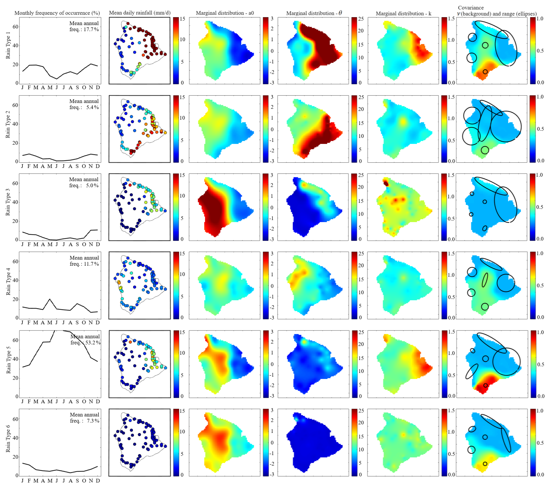
Figure 3 Daily rainfall patterns of the six rain types of the Island of Hawai`i and associated model parameters. Different rows denote different rain types. The first column shows the seasonality of rain type occurrence, column 2 displays the mean daily rainfall, columns 3–5 display maps of the estimated marginal parameters, and column 6 displays maps of the estimated covariance parameters, namely the shape parameter ν of the covariance function (background color) and ellipses of anisotropy (overprint) that denote the value of the range parameters ρ_a and ρ_b for different directions and for each climate division.

4.2 Stochastic generation of orographic rainfall

4.2.1 Multi-site rainfall simulation

We first assess the ability of the NSTG model to capture and reproduce the statistical signature of rainfall at gauge locations, which corresponds to setting-up and deploying a multi-site stochastic rainfall generator. Synthetic rainfall is generated by stochastic simulation (cf. Sect. 3.4) performed on an irregular grid whose nodes are the locations of the rain gauges. For comparison purposes the simulation is repeated the same number of times as the number of days within each rain type, and the 7305 daily simulations are ordered and concatenated to create a single 20-year time series with the same rain type timeline as the observations. Section S1 in the Supplement displays the seasonality and inter-annual variability of the 20-year time series simulated at the six locations used in Fig. 2 to investigate the diversity of rainfall climatology over the Island of Hawai`i, and shows that the NSTG model coupled with rain types is able to reproduce rainfall seasonality and inter-annual variability across the island.

To explore the spatial patterns of daily rainfall emerging from the simulations, the statistical distribution of the simulated daily rainfall is subsequently mapped and compared to the distribution of observations. The following statistics are used to assess the distribution of rainfall at each site: the mean daily rainfall, the frequency of rainfall occurrence, the median of daily rainfall during wet days (with wet days defined at the rain gauge level, i.e., the day d is considered as wet at location s if $R(\mathit{s},d)>\mathrm{0}$), and the quantile 95 % of daily rainfall during wet days. In addition, the whole distributions of simulations and observations are compared at each location using the 1-Wasserstein distance (Panaretos and Zemel, 2019; Vissio et al., 2020):

$$\begin{array}{}\text{(9)}& W_{\mathrm{1}}({\mathit{R}}_{\mathrm{obs}},{\mathit{R}}_{\mathrm{sim}})=\sum _{i=\mathrm{1}}^n|{\mathit{R}}_{\mathrm{obs}\left(i\right)}-{\mathit{R}}_{\mathrm{sim}\left(i\right)}|\end{array}$$

where R_obs(i) (resp. R_sim(i)) is the element of rank i of the vector R_obs (resp. R_sim).

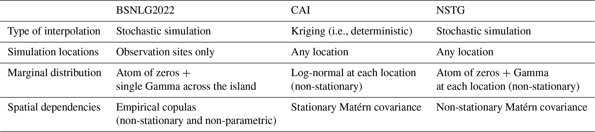
The performance of the NSTG model is benchmarked against the model of Benoit et al. (2022), hereafter refereed to as BSNLG2022. BSNLG2022 is a multi-site stochastic rainfall generator that has been designed specifically for tropical islands with complex topography. It draws on rain types to model the temporal evolution of rainfall statistics and on a combination of empirical copulas and Gamma distribution to model the multi-site distribution of rainfall conditional to rain types (see Appendix C for a comparison between BSNLG2022 and the trans-Gaussian model of this study). In the following the BSNLG2022 model is calibrated using the same training dataset and the same rain type time series as the ones used to calibrate the NSTG model.

Figure 4 compares the pointwise statistical signature of rainfall observations for the period 2000–2019 with the one of the 20-year synthetic rainfall simulations performed by the NSTG model (see Sect. S2 for a comparison stratified by rain types) and by the BSNLG2022 benchmark model. Results show that both models reproduce very well the four diagnostic statistics, and that the NSTG model slightly outperforms BSNLG2022 in terms of 1-Wasserstein distance with observations, in particular in places where the gradients of rainfall statistics are the strongest (i.e., the northern and eastern endpoints of the island). The only area where the proposed model is less effective than BSNLG2022 is on the East side of the island where the density of rain gauges is the highest. In this area one can notice that the NSTG model does not perfectly captures the strong variability of rain statistics between very nearby locations, and tends to slightly over-smooth rainfall statistics in space. This can be explained by the inclusion of a nugget term in the Kriging system used to interpolate the parameters of the transform function Ψ (cf. Sect. 3.3), which is necessary to filter local errors during the interpolation but leads to parameter maps that do not exactly honor point parameter estimates, and therefore results in rainfall simulations that do not perfectly reproduce rainfall statistics at observation locations. Apart for this minor over-smoothing of rain statistics in densely gauged areas, the NSTG model is able to simulate synthetic multi-site daily rainfall events that closely mimic observations.

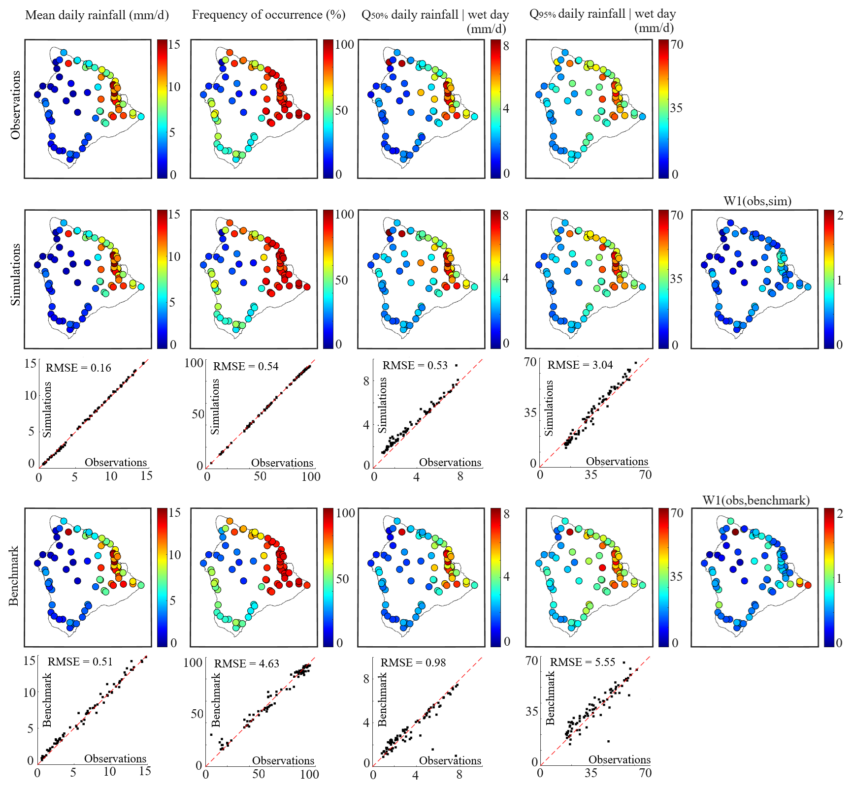
Figure 4 Statistical signature of rainfall derived from observations (first row), stochastic simulations performed by the NSTG model (second row), and stochastic simulations performed by the BSNLG2022 benchmark model (fourth row). The third (resp. fifth) row displays the scatter-plots of the observed versus simulated (resp. benchmark simulation) statistics of interest as well as the associated Root Mean Square Error (RMSE). The first column displays the mean daily rainfall, column 2 displays the frequency of rainfall occurrence, columns 3 and 4 display the quantiles 50 % and 95 % of daily rainfall during wet days, and column 5 displays the 1-Wasserstein distance between observations and simulations.

4.2.2 Rainfall fields simulation

The NSTG model has the ability to simulate rainfall not only at gauge locations, but also across the whole domain of interest 𝒟. To assess this ability to simulate spatially continuous rainfall fields, the NSTG model is set-up to simulate rainfall on a 2 km-resolution regular grid. In contrast, the BSNLG2022 benchmark model remains multi-site because it is by construction unable to interpolate rainfall between observation locations (due to the use of empirical copulas – cf. Appendix C – the spatial dependencies can only be modeled between locations where observations are available).

Synthetic rainfall is generated by stochastic simulation (cf. Sect. 3.4). As in Sect. 4.2.1 the simulation is repeated the same number of times as the number of days within each rain type, and the 7305 daily simulations are ordered and concatenated to create a single 20-year time series with the same rain type timeline as the observations. To explore the performance of the simulations to generate realistic spatial patterns of rainfall, we map the similarity of rainfall time series simulated at three specific locations with the time series simulated in the rest of the target area. We also look at scatter-plots of similarity statistics between all pairs of rain gauge locations to assess spatial patterns at the scale of the island. The similarity of time series of rainfall occurrence is quantified by the Jaccard Index of Rainfall Occurrence (JI-RO) (Jaccard, 1901), while the similarity of time series of rainfall intensity is quantified by the Pearson Correlation Coefficient of Rainfall Intensity (PCC-RI, evaluated solely on wet days):

$$\begin{array}{}\text{(10)}& {\displaystyle }\begin{array}{rl}& \text{JI-RO}({\mathit{s}}_i,{\mathit{s}}_j)={\displaystyle \frac{M_{\mathrm{11}}}{M_{\mathrm{01}}+M_{\mathrm{10}}+M_{\mathrm{11}}}}\mathrm{with}:\\ & M_{\mathrm{11}}=\sum _{t=\mathrm{1}}^{N_{\mathrm{T}}}\textcolor{red}{}\left[R({\mathit{s}}_i,t)>\mathrm{0}\right]\cdot \textcolor{red}{}\left[R({\mathit{s}}_j,t)>\mathrm{0}\right]\\ & M_{\mathrm{01}}=\sum _{t=\mathrm{1}}^{N_{\mathrm{T}}}\textcolor{red}{}\left[R({\mathit{s}}_i,t)=\mathrm{0}\right]\cdot \textcolor{red}{}\left[R({\mathit{s}}_j,t)>\mathrm{0}\right]\\ & M_{\mathrm{10}}=\sum _{t=\mathrm{1}}^{N_{\mathrm{T}}}\textcolor{red}{}\left[R({\mathit{s}}_i,t)>\mathrm{0}\right]\cdot \textcolor{red}{}\left[R({\mathit{s}}_j,t)=\mathrm{0}\right]\end{array}\text{(11)}& {\displaystyle }\begin{array}{rl}& \mathrm{PCC}-\mathrm{RI}({\mathit{s}}_i,{\mathit{s}}_j)\\ & ={\displaystyle \frac{{\sum }_{t_{\mathrm{w}}=\mathrm{1}}^{N_{\mathrm{w}}}\left(R({\mathit{s}}_i,t_{\mathrm{w}})-\stackrel{\mathrm{‾}}{R}\left({\mathit{s}}_i\right)\right)\left(R({\mathit{s}}_j,t_{\mathrm{w}})-\stackrel{\mathrm{‾}}{R}\left({\mathit{s}}_j\right)\right)}{\sqrt{{\sum }_{t_{\mathrm{w}}=\mathrm{1}}^{N_{\mathrm{w}}}{\left(R({\mathit{s}}_i,t_{\mathrm{w}})-\stackrel{\mathrm{‾}}{R}\left({\mathit{s}}_i\right)\right)}^{\mathrm{2}}}\sqrt{{\sum }_{t_{\mathrm{w}}=\mathrm{1}}^{N_{\mathrm{w}}}{\left(R({\mathit{s}}_j,t_{\mathrm{w}})-\stackrel{\mathrm{‾}}{R}\left({\mathit{s}}_j\right)\right)}^{\mathrm{2}}}}}\\ & \mathrm{with}\stackrel{\mathrm{‾}}{R}\left({\mathit{s}}_i\right)={\displaystyle \frac{\mathrm{1}}{N_{\mathrm{w}}}}\sum _{t_{\mathrm{w}}=\mathrm{1}}^{N_{\mathrm{w}}}R({\mathit{s}}_i,t_{\mathrm{w}})\\ & \mathrm{and}\stackrel{\mathrm{‾}}{R}\left({\mathit{s}}_j\right)={\displaystyle \frac{\mathrm{1}}{N_{\mathrm{w}}}}\sum _{t_{\mathrm{w}}=\mathrm{1}}^{N_{\mathrm{w}}}R({\mathit{s}}_j,t_{\mathrm{w}})\end{array}\end{array}$$

where N_T is the number of days in the dataset (here N_T=7305), N_w is the number of wet days, and $\textcolor{red}{}[.]$ is the indicator function that takes the value 1 if the event in brackets is true and 0 otherwise.

Figure 5 compares the spatial structure of rainfall observations with those of the synthetic rainfall datasets simulated by the NSTG model on one hand (see Sect. S2 for a comparison stratified by rain types), and of the BSNLG2022 benchmark model on the other hand. Results show that when focusing on the ability of the models to reproduce the spatial patterns of rainfall occurrence evaluated through JI-RO (Fig. 5a, b, e, f), both models perform equally well and almost perfectly simulate these patterns. Focusing next on the spatial patterns of rainfall intensity during rainy days evaluated through PCC-RI (Fig. 5c, d, g, h), one can notice that the BSNLG2022 benchmark model simulates them very well while the NSTG model presents a few imperfections, with some correlations of moderate intensity being underestimated (Fig. 5g). Underestimated spatial correlations mostly involve pairs of locations that are far from each others, and are apparent at the South-East of the island in Fig. 5c (top row), and also detectable at the North-East of the island in Fig. 5c (top row) and at the East of the island in Fig. 5c (bottom row). This imperfect modeling of some long range correlations is likely due to the use of relatively large climate divisions when estimating the parameters of the covariance function at the local scale, which is necessary in the present setting to ensure that enough observations are available for a robust estimation of the covariance parameters (cf. Sect. 3.3). The interpolation of these parameters to build an island-scale non-stationary covariance function can misrepresent the actual values in areas where the covariance parameters vary strongly in space as well as at the edge of the climate divisions, leading to an imperfect modeling of the spatial dependencies in these areas. The spatial interpolation of the covariance parameters could be improved by extending the rain gauge network in poorly gauged locations, and in turn defining smaller climate divisions. The densification of the rain gauge network may also provide more detailed insights on the patterns of spatial dependencies, which could call for the use of a more refined covariance model accounting for instance for barrier effects (Bakka et al., 2019) that may be induced by the drying effect of the TWI in the center of the island. On the positive side, the short to medium range correlations are very well simulated by the trans-Gaussian model, including the patterns of non-stationarity and anisotropy. One should in particular notice the ability of the model to simulate sinuous contours of iso-correlation (i.e., not circular nor elliptic) in Fig. 5c, which is made possible by the use of a non-stationary and anisotropic covariance function to model spatial dependencies within the latent field. In addition, Fig. 5g shows that the NSTG model properly simulates medium to strong correlations (Pearson correlation > 0.5) for all pairs of gauges, which is of particular importance for rainfall mapping because they are the ones that influence the most the spatial interpolation.

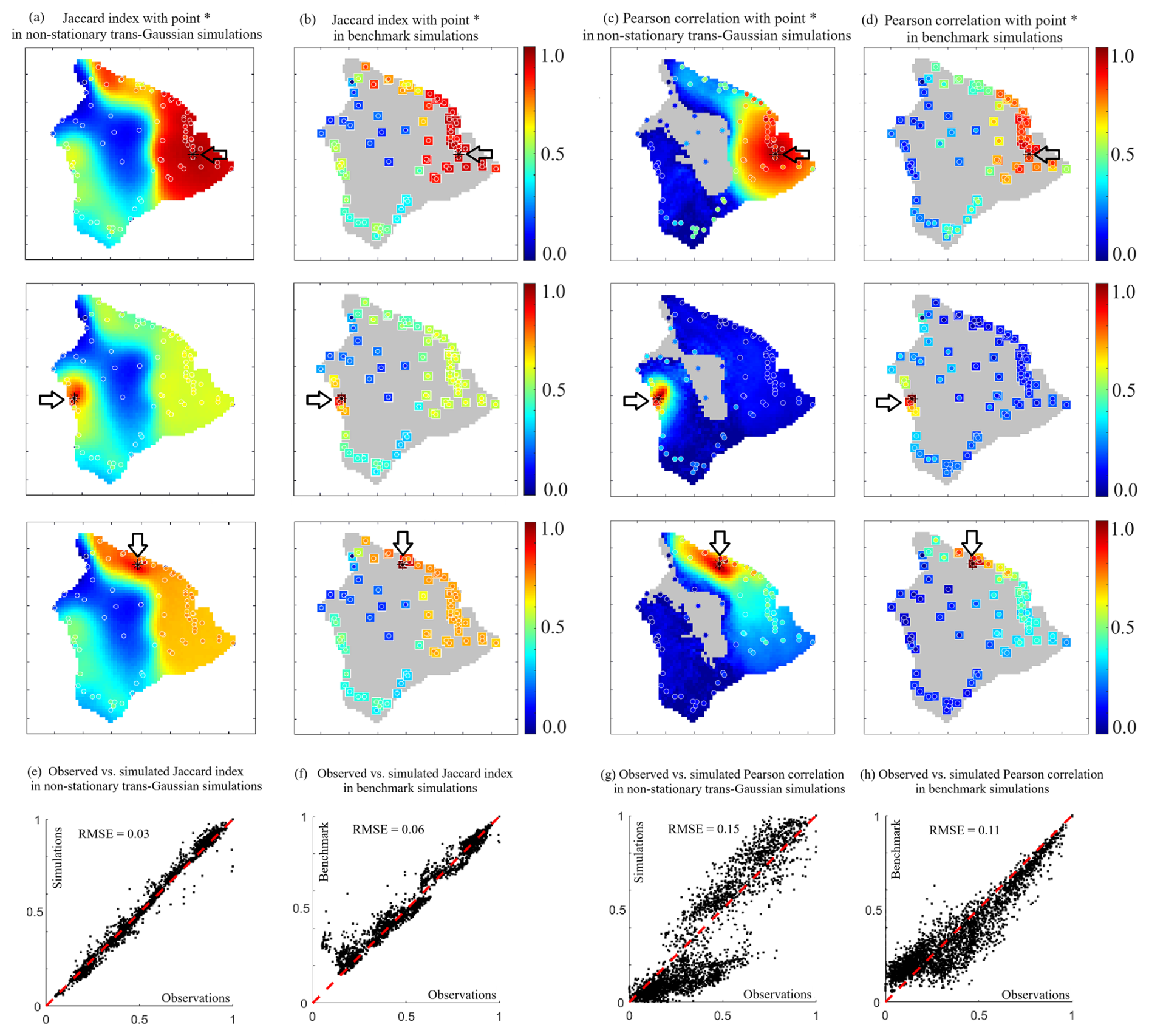
Figure 5 Spatial patterns of rainfall generated by stochastic simulations performed by the NSTG model (a, c, e, g) and by the BSNLG2022 benchmark model (b, d, f, h). The panels (a) and (b) display the Jaccard Index of rainfall occurrence (JI-RO) with respect to three locations denoted by a star (^*), and the panels (c) and (d) display the Pearson Correlation Coefficient of rain intensity evaluated solely on wet days (PCC-RI) with respect to the same locations. The panel (e) (resp. f) displays scatter-plots of observed versus simulated Jaccard index for all pairs of rain gauge locations for the NSTG model (resp. the BSNLG2022 benchmark model). The panel (g) (resp. h) displays scatter-plots of observed versus simulated Pearson correlation for all pairs of rain gauge locations and for the NSTG model (resp. the BSNLG2022 benchmark model). In (c) the grey color denotes areas where less than 5 % of the days are wet simultaneously with the target location, and where the estimation of PCC-RI is therefore deemed unrealiable. In (a), (b), (c), (d) the foreground circles denote observation data, the continuous background color (in a, c) denotes simulations from NSTG model, and the background squares (in b, d) denote simulations from the BSNLG2022 benchmark model.

In summary, Fig. 4 shows that the NSTG model is able to simulate rainfall fields with point statistics reproducing almost perfectly the marginal distribution of the observations. Figure 5 shows that the NSTG model can simulate rainfall fields with realistic patterns of rainfall occurrence and intensity, and is in particular able to reproduce the sinuous contours of iso-correlation emerging from the Hawai`i observation dataset. The use of a parametric covariance function is the keystone for the design of a stochastic rainfall generator able to simulate spatially continuous rainfall fields, which is a requirement to generate rainfall maps from sparse rain gauge observations as detailed hereafter.

4.3 Mapping daily rainfall over complex topography

Building on the ability of the NSTG model to simulate realistic rainfall fields between observation locations, we next assess its ability to predict rainfall at ungauged locations, which corresponds to rainfall mapping. This is evaluated through a cross-validation procedure, in which we iteratively select a target rain gauge, remove it from the training dataset (as well as the data from all gauges belonging to a 5 km-radius circular area centered on this target gauge in order to mitigate the effect of near co-located gauges), re-estimate model parameters for the new training dataset, predict rainfall at the target location, and finally compare the predicted and observed rainfall values. The same procedure is applied to all gauges sequentially, and ultimately the cross-validation implemented here is equivalent to a leave-one-out approach. The quality of the rainfall prediction is evaluated with respect to the ability of the model to estimate rainfall occurrence as well as rainfall intensity during wet days. The prediction of rainfall occurrence is evaluated at each gauge location through the following metrics: the mean bias of the predicted rainfall occurrence (MB-RO), the mean absolute error of rainfall occurrence (MAE-RO), and the Brier score of rainfall occurrence (BS-RO) that measures the accuracy of the probabilistic prediction (Brier, 1950):

$$\begin{array}{}\text{(12)}& {\displaystyle }\begin{array}{rl}& \text{MB-RO}\left(\mathit{s}\right)\\ & ={\displaystyle \frac{\mathrm{1}}{N_{\mathrm{T}}}}\sum _{t=\mathrm{1}}^{N_{\mathrm{T}}}(\textcolor{red}{}\left[\widehat{R}(\mathit{s},t)>\mathrm{0}\right]-\textcolor{red}{}\left[R_{\mathrm{obs}}(\mathit{s},t)>\mathrm{0}\right])\end{array}\text{(13)}& {\displaystyle }\begin{array}{rl}& \text{MAE-RO}\left(\mathit{s}\right)\\ & ={\displaystyle \frac{\mathrm{1}}{N_{\mathrm{T}}}}\sum _{t=\mathrm{1}}^{N_{\mathrm{T}}}|\textcolor{red}{}\left[\widehat{R}(\mathit{s},t)>\mathrm{0}\right]-\textcolor{red}{}\left[R_{\mathrm{obs}}(\mathit{s},t)>\mathrm{0}\right]|\end{array}\text{(14)}& {\displaystyle }\begin{array}{rl}& \text{BS-RO}\left(\mathit{s}\right)\\ & ={\displaystyle \frac{\mathrm{1}}{N_{\mathrm{T}}}}\sum _{t=\mathrm{1}}^{N_{\mathrm{T}}}\left({\displaystyle \frac{\mathrm{1}}{N_{\mathrm{sim}}}}\right(\sum _{\mathrm{sim}=\mathrm{1}}^{N_{\mathrm{sim}}}\textcolor{red}{}\left[R_{\mathrm{sim}}\right(\mathit{s},t)>\mathrm{0}])-\textcolor{red}{}\left[R_{\mathrm{obs}}(\mathit{s},t)>\mathrm{0}\right]{)}^{\mathrm{2}}\end{array}\end{array}$$

where $\widehat{R}(\mathit{s},t)$ is the prediction of rainfall at location s and day t (here the median of 100 simulations is selected as rainfall prediction for the NSTG model), and N_sim is the number of conditional simulations (here N_sim=100). To complement the evaluation of rainfall occurrence prediction, we assess the prediction of rainfall intensity conditionally to the occurrence of rainfall (in the following, the occurrence of rainfall is always determined from observations). The prediction of rainfall intensity during wet days is evaluated through the following metrics, evaluated solely on wet days: the mean bias of the predicted intensity (MB-RI), the mean absolute error of rainfall intensity (MAE-RI), and the mean continuous ranked probability score of rainfall intensity (MCRPS-RI, (Gneiting and Raftery, 2007)) that measures the accuracy of the probabilistic prediction and corresponds to the integral of the Brier score associated with all possible rainfall intensity thresholds greater than zero:

$$\begin{array}{}\text{(15)}& {\displaystyle }\mathrm{MB}-\mathrm{RI}\left(\mathit{s}\right)={\displaystyle \frac{\mathrm{1}}{N_{\mathrm{w}}}}\sum _{t_{\mathrm{w}}=\mathrm{1}}^{N_{\mathrm{w}}}\left(\widehat{R}(\mathit{s},t_{\mathrm{w}})-R_{\mathrm{obs}}(\mathit{s},t_{\mathrm{w}})\right)\text{(16)}& {\displaystyle }\mathrm{MAE}-\mathrm{RI}\left(\mathit{s}\right)={\displaystyle \frac{\mathrm{1}}{N_{\mathrm{w}}}}\sum _{t_{\mathrm{w}}=\mathrm{1}}^{N_{\mathrm{w}}}\left|\widehat{R}(\mathit{s},t_{\mathrm{w}})-R_{\mathrm{obs}}(\mathit{s},t_{\mathrm{w}})\right|\text{(17)}& {\displaystyle }\begin{array}{rl}& \mathrm{MCRPS}-\mathrm{RI}\left(\mathit{s}\right)\\ & ={\displaystyle \frac{\mathrm{1}}{N_{\mathrm{w}}}}\sum _{t_{\mathrm{w}}=\mathrm{1}}^{N_{\mathrm{w}}}\underset{r=\mathrm{0}}{\overset{+\mathrm{\infty }}{\int }}\left({\mathrm{F}}_{R_{\mathrm{sim}}(\mathit{s},t_{\mathrm{w}})}\right(r)-\textcolor{red}{}[r\ge R_{\mathrm{obs}}(\mathit{s},t_{\mathrm{w}})]{)}^{\mathrm{2}}\mathrm{d}r\end{array}\end{array}$$

where N_w is the number of wet days observed at the target location (i.e., days such that $R_{\mathrm{obs}}(\mathit{s},t_{\mathrm{w}})>\mathrm{0}$), and ${\mathrm{F}}_{R_{\mathrm{sim}}(\mathit{s},t_{\mathrm{w}})}$ is the cdf of the rainfall forecast derived from the 100 simulations R_sim(s,t_w).

The performance of the NSTG model is benchmarked against a Climatically Aided Interpolation (CAI) framework (Willmott and Robeson, 1995; Hunter and Meentemeyer, 2005), which has been applied to map monthly rainfall in Hawai`i (Lucas et al., 2022) and is customized hereafter to enable the mapping of daily rainfall. CAI is used in place of BSNLG2022 to benchmark rainfall mapping because the latter model only allows for multi-site modeling and therefore lacks the interpolation skills necessary for mapping. CAI involves firstly to derive a mean Climatological Rainfall Pattern (CRP) at each gauge location for the period of interest, secondly to define RainFall Anomalies (RFA) to the CRP, thirdly to interpolate CRP and RFA at ungauged locations, and fourthly to retrieve the interpolated rainfall fields by back-transformation of RFA. To allow a fair comparison with the NSTG model, one CAI model is set up for each rain type separately and the exact same dataset is used for model calibration. In this setting and for a given rain gauge location ${\mathit{s}}_{\mathrm{g}}\in {\mathcal{N}}_{\mathrm{etwork}}\subset \mathcal{D}$ we define the CRP as the mean daily rainfall during the rain type of interest (i.e., $\mathrm{CRP}\left({\mathit{s}}_{\mathrm{g}}\right)=\frac{\mathrm{1}}{N_{\mathrm{obs}}}{\sum }_{j=\mathrm{1}}^{N_{\mathrm{obs}}}\left(R_j\left({\mathit{s}}_{\mathrm{g}}\right)\right)$), and the RFA of a given day j as: ${\mathrm{RFA}}_j\left({\mathit{s}}_{\mathrm{g}}\right)=\log \left(\frac{R_j\left({\mathit{s}}_{\mathrm{g}}\right)}{\mathrm{CRP}\left({\mathit{s}}_{\mathrm{g}}\right)}+\mathrm{1}\right)$. The interpolation of the CRP at ungauged locations is performed by Ordinary Kriging using a stationary Matérn covariance function with Nugget, and the interpolation of RFA is performed by Ordinary Kriging using a stationary Matérn covariance function without Nugget. With the above definitions the CAI model can be understood as a deterministic spatial interpolator (i.e., it provides a single estimation of daily rainfall at each target location, which is in contrast with stochastic interpolation that provides an ensemble prediction), which accounts for the non-stationarity of rainfall marginal distribution through the CRP, but assumes a stationary covariance for the spatial interpolation.

Figure 6a–d displays the results of the cross-validation focusing on the spatial prediction of rainfall occurrence. It shows that the NSTG model performs very well except for a few stations located in sparsely gauged areas and at the transition between a domain where rainfall is very frequent (North-East coast and mountain slopes) and another domain with very rare precipitation (summits in the center of the island and North-West coast). In that context, the withdrawal of the target rain gauge from the training and conditioning datasets leads to a lack of information about the exact location of the gradient of rainfall occurrence, and in the absence of such information the model generates a smooth transition which misrepresents the actual gradient. This artifact is absent from more densely gauged areas (e.g., the West and North-East coasts), and one can therefore infer that the density of the rain gauge network is crucial to get accurate rain occurrence maps in areas with strong rainfall gradients. When comparing the above results with the CAI, one can notice that the NSTG model outperforms the CAI benchmark model both in terms of bias (Fig. 6b) and magnitude of the prediction errors (Fig. 6c). This can be explained by the tendency of the CAI benchmark model to over-predict very light rain in place of dry conditions because it does not explicitly account for the zero-inflated nature of daily rainfall data. In contrast, the explicit modeling of this feature in the trans-Gaussian framework allows the NSTG model to map rainfall occurrence more effectively.

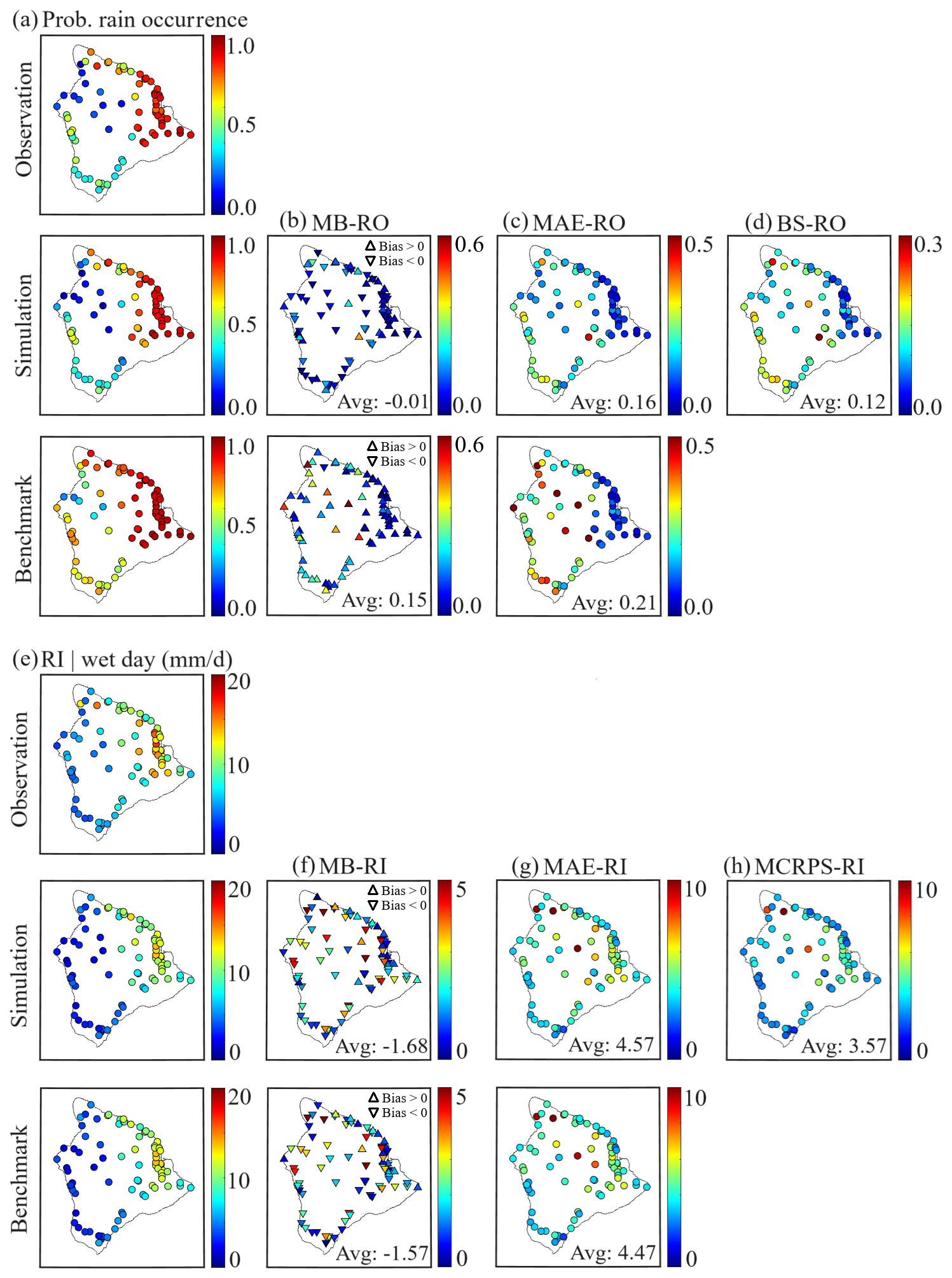
Figure 6 Cross-validation assessment of rainfall mapping performance. (a–d) Evaluation of rain occurrence prediction. (e–h) Evaluation of the prediction of daily rainfall intensity conditionally to the occurrence of rainfall.

Figure 6e–h investigates the interpolation of rainfall intensity conditionally to the occurrence of rainfall. One can notice that in contrast with rainfall occurrence, rainfall intensity varies substantially between nearby locations, which is particularly visible in the densely gauged area in the East of the island (Fig 6e). This feature is not perfectly captured by the NSTG model nor by the CAI benchmark model, and both models smooth-out the local variability of rainfall intensity. This is because all data from the gauges located in a 5km radius around the target gauge are discarded from the cross-validation, which prevents the models from learning the local behavior of rainfall and leads to biases of opposite signs for neighbouring gauges (Fig 6f). The second artefact in rainfall intensity mapping is the imperfect depiction of rainfall intensity gradients in sparsely gauged areas, which is caused by the same reasons as discussed for rainfall occurrence. When comparing the skills of the two rainfall mapping approaches, one can notice that the CAI benchmark model marginally outperforms the NSTG model when averaging the MB-RI and MAE-RI metrics over all gauges, but that the patterns and overall magnitude of the interpolation errors are very similar for both models. This suggests that using a non-stationary covariance in the NSTG model does not improve rainfall mapping in sparsely gauged areas, even though the non-stationary covariance effectively improves the realism of the stochastic rainfall field simulations (cf. Sect. 4.2.2) used as a basis for the stochastic interpolation.

On another note, Fig. 6d and h show that a significant advantage of the NSTG model is its ability to provide probabilistic estimates of rainfall by means of an ensemble of conditional simulations, which CAI cannot do. The better scores obtained for the probabilistic forecasts (BS-RO in Fig. 6d, and MCRPS-RI in Fig. 6h) than for their deterministic counterparts (MAE-RO in Fig. 6c, and MAE-RI in Fig. 6g) show the additional information brought by the ensemble approach.

4.4 Conditioning daily rainfall maps to monthly totals

Section 4.3 showed that, like every interpolation method, the NSTG model has decreasing skills in rainfall mapping when the density of the rain gauge network decreases. This is often unavoidable in mountainous regions because the rough topography makes the setup and maintenance of rain gauge networks challenging. To improve the representation of rainfall gradients in poorly gauged areas, we propose conditioning daily rainfall maps not only to daily rain gauge observations as demonstrated in Sect. 4.3, but also to monthly totals derived from monthly rainfall maps that incorporate more information about rainfall patterns than is provided by the daily rain gauge network.

Conditioning daily maps to monthly totals is obtained by adding a Metropolis within Gibbs step in the processing framework (see Sect. 3.6), and hereafter we apply this step at 200 virtual stations spread throughout the Island of Hawai`i (white crosses in Fig. 7, bottom left) to compensate for the large gaps existing in the rain gauge network. The impact of conditioning daily rainfall maps to monthly totals is illustrated for the months of January, April, July and October 2018, which have been selected to cover a wide range of weather conditions and sample all rain types observed in Hawai`i.

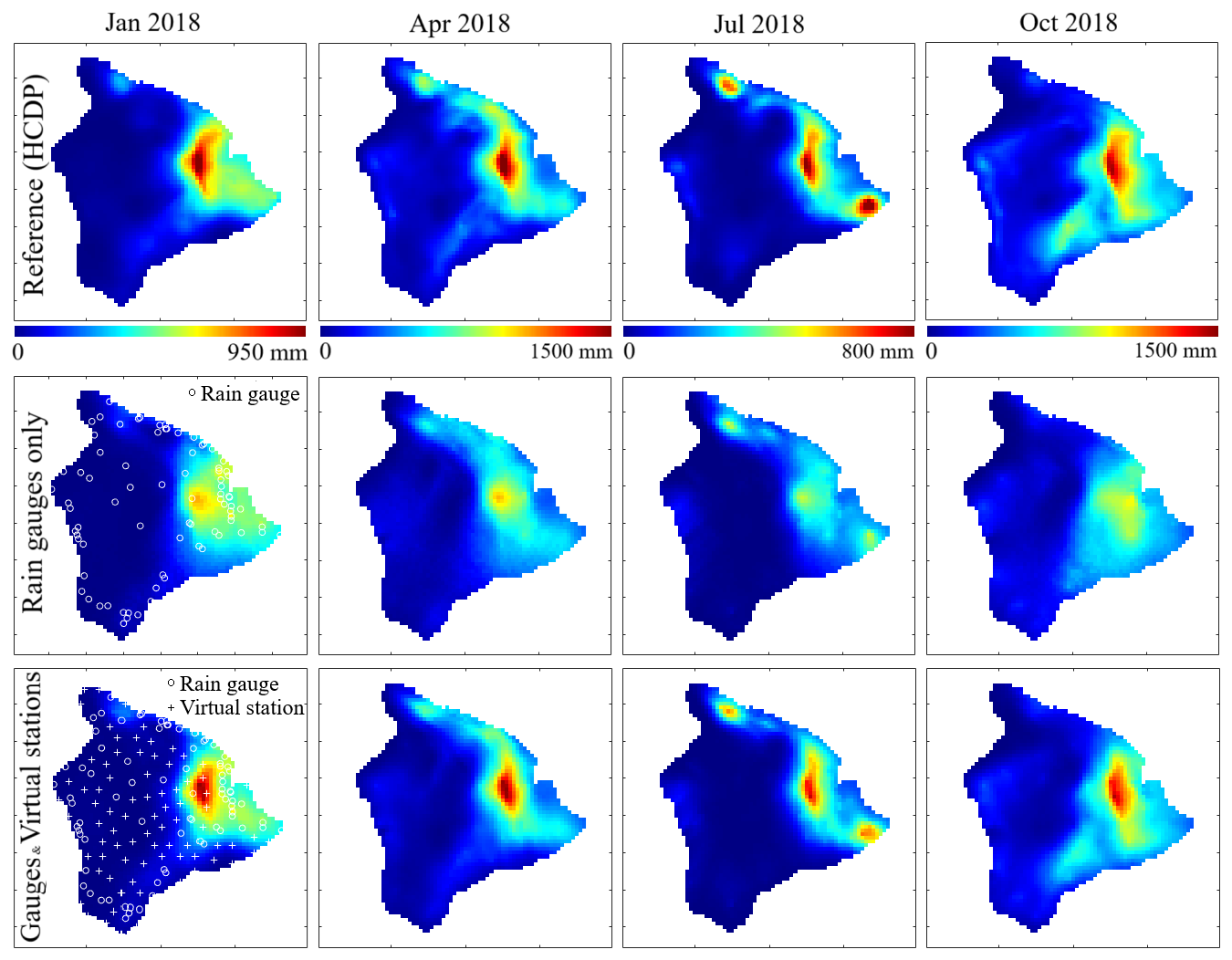
Figure 7 Maps of monthly rainfall for the months of January, April, July and October 2018 derived from the HCDP monthly historical rainfall dataset (top row), the sum of 30 or 31 daily rainfall maps obtained by the stochastic interpolation of rain gauge observations (middle row), and the sum of daily rainfall maps obtained by the stochastic interpolation of rain gauge observations constrained to honor HCDP monthly totals at 200 virtual stations (bottom row). In the bottom plot of January 2018 the dots denote the locations of the 79 rain gauges and the crosses denote the locations of the 200 virtual stations.

Figure 7 compares the reference HCDP monthly rainfall maps (Fig. 7, top row) with the monthly accumulations obtained by summing the 30 or 31 daily rainfall maps derived from daily rain gauge observations only (Fig. 7, middle row), and with the sum of daily maps also conditioned to HCDP monthly totals at 200 virtual stations (Fig. 7, bottom row). The daily rainfall fields associated to Fig. 7 middle row and Fig. 7 bottom row are displayed in Sect. S3–S6. Results show that conditioning daily rainfall maps to monthly totals enables to transpose the features of the reference HCDP maps into the daily rainfall maps derived from rain gauge observations, and in their monthly sum displayed in Fig. 7 bottom row. In particular, one can notice in Fig. 7 bottom row the emergence of a monthly spatial maximum at an ungauged location that is located on the East side of Mauna Loa for the four months of interest. In addition, the spatial gradients of rainfall occurring in the North and South of this wet area are sharper when the daily maps are conditioned to monthly totals, leading to more realistic rainfall patterns in the South-East and East feet of Mauna Loa. At higher altitudes, the wet-dry gradient occurring at the East of Mauna Kea and Mauna Loa summits is more sinuous when adding the monthly conditioning, which again improves the realism of the monthly rainfall patterns. It is worth mentioning that the improved gradients and patterns of monthly rainfall obtained by conditioning daily maps to monthly totals propagate to the daily rainfall maps displayed in Sect. S3–S6 in supplementary material, and that this improvement does not introduce any spurious smoothing nor a drizzle effect (i.e., the under-estimation of dry areas coupled with an over-estimation of very low rainfall intensities) in the daily rainfall maps.

To assess how the conditioning to monthly totals impacts daily rainfall maps, we perform a cross-validation study narrowed to three gauges located on the East side of Mauna Kea and on the months of January, April, July and October 2018. This area has been selected because it experiences a strong spatial gradient of rainfall and because it is only sparsely gauged, which leads to a limited performance in rainfall mapping as discussed in Sect. 4.3. The cross-validation is performed as in Sect. 4.3 and we use the same evaluation metrics (i.e., Mean Bias – MB, Mean Absolute Error - MAE, and Mean Continuous Ranked Probability Score – MCRPS) but for conciseness these metrics are evaluated hereafter on a monthly basis and on the entire time series (i.e., without separation between rainfall occurrence and rainfall intensity). We compare three methods of rainfall mapping: (1) the stochastic interpolation of daily rain gauge observations with the parameters of the NSTG model assumed to be unknown at the target location, which corresponds to the setting tested in Sect. 4.3; (2) the stochastic interpolation of daily rain gauge observations with the parameters of the NSTG model assumed to be known at the target location, which corresponds to the hypothetical case of a rain gauge that has been discontinued but whose past data are used to estimate the parameters of the model at that location; (3) the stochastic interpolation of daily rain gauge observations with the parameters of the NSTG model assumed to be unknown at the target location, and with an additional conditioning to the monthly total derived from the HCDP reference map.

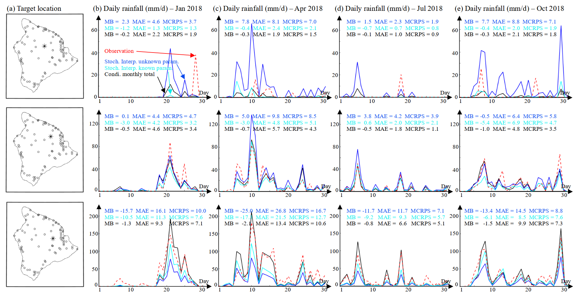
Figure 8 Cross-validation assessment of the conditioning of daily rainfall maps to monthly totals. (a) Location of the three gauges of interest. (b–e) Time series of observed (dashed red lines) and interpolated (solid lines) daily rainfall for the three target locations and the months of January, April, July and October 2018. In (b)–(e) the dark blue lines denote results of stochastic interpolation with unknown model parameters at target location, the light blue lines denote results of stochastic interpolation with known model parameters at target location, and the black lines denote results of stochastic interpolation with unknown model parameters at target location and with additional conditioning to the monthly total.

Figure 8 displays the results of the cross-validation for the three settings described above. Results show that the conditioning to monthly totals (black lines in Fig. 8) drastically improves the stochastic interpolation when the parameters of the model are unknown at the target location (dark blue lines in Fig. 8). The improvement is major for the mean bias (90 % overall improvement) because the conditioning to monthly totals forces the mean monthly bias to be near zero, and the improvement is also very substantial for the mean absolute error (46 % overall improvement) and the mean CRPS (44 % overall improvement). This proves that conditioning to monthly totals not only improves the spatial patterns of rainfall embedded in monthly and daily maps as shown in Fig. 7 and in Sect. S3–S6, but also substantially improves point prediction – that is, the actual quality of the daily rainfall maps. It is also worth noticing that in the case of a sparsely gauged area the conditioning to monthly totals leads to better results than knowing the true value of model parameters (light blue lines in Fig. 8), with an overall improvement of 83 % for the mean bias, 15 % for the mean absolute error, and 13 % for the mean CRPS. This suggests that knowing the local monthly rainfall accumulation brings more information to the stochastic interpolation of daily observations than knowing the long term rainfall statistics at the target location, and supports the idea that combining different temporal resolutions (here daily and monthly) in rainfall mapping effectively improve the high-resolution maps while ensuring consistency between maps at different resolutions.

5 Conclusions

In this study we designed a fully non-stationary and trans-Gaussian model that is able to accommodate the steep spatial gradients of daily rainfall observed in mountainous regions. The use of a non-stationary transform function enables the simulation of realistic patterns of daily rainfall occurrence and intensity. In addition, the use of an anisotropic and non-stationary covariance function for the latent field paves the way for the simulation of rainfall fields with realistic spatial dependencies. When applied to data from a network of 79 rain gauges on the Island of Hawai`i, the proposed model is able to infer the spatial distribution of orographic rainfall and simulate gridded rainfall products that skillfully reproduce the observed rainfall statistics. Finally, daily rainfall maps are improved in poorly gauged areas by conditioning rainfall interpolation not only to daily rain gauge observations, but also to monthly totals through a Metropolis within Gibbs approach.

When designing the geostatistical model, we chose to follow a data-driven approach using only observations to inform the non-stationarity of rainfall. Hence, the marginal distribution of rainfall is first estimated at each rain gauge location separately and subsequently interpolated at ungauged locations. Similarly, the covariance function of the latent field is first assumed to be stationary within relatively small climate divisions during the estimation of the covariance parameters, then the covariance parameters are assigned to the barycenter of each climate division, and finally these parameters are interpolated through space and incorporated in a model of non-stationary covariance. The choice of a data-driven non-stationary model has the advantage of removing the need for covariates such as elevation or wind to inform the patterns of rainfall non-stationarity. This is of particular interest over complex topography and for high-resolution rainfall modeling because in this context the link between rainfall and topo-climatic covariates tends to be weak and complex (Giambelluca et al., 2013; Benoit et al., 2024) and therefore challenging to account for in statistical rainfall models. However, data-driven non-stationary models require a lot of observations for calibration, which restricts the use of our model to densely gauged areas and calls for an increased density of rain gauge networks to improve model performance. Such high-density rain gauge network is currently being implemented in the state of Hawaii by the extension of the HCDP weather station network through the construction of Hawai`i Mesonet (Longman et al., 2024).

Over the past few decades, automatic rain gauges and weather stations have started to record rainfall data at sub-daily time steps and large observation datasets at a 10 min (and sometimes higher) temporal resolution have become common. Generating high-temporal-resolution rainfall maps at the scale of an island or a mountain range using such rain gauge observations could be addressed using trans-Gaussian stochastic rainfall models. The main difficulty we envision in this endeavor is the modeling of the temporal dependencies that emerge in sub-daily resolution rainfall fields in addition to the spatial dependencies addressed in the present study that focused on daily resolution. Accounting for both spatial and temporal dependencies in the presence of orographic effects will require the development of non-stationary space-time covariance functions to model the latent field (Allard et al., 2025) and robust estimation methods to infer model parameters from rain gauge observations.

In the end, rainfall maps derived from rain gauge observations are expected to complement radar rainfall estimates in mountainous regions where the complex topography challenges this technology with beam blocking and ground clutter, and to substitute the lack of radar products in non-equipped areas. Increasing the accuracy and resolution of rainfall maps is expected to improve hydrological modeling and flood forecasting in small catchments that are widespread in mountainous regions where orographic effects prevail.

Appendix A: Gibbs sampler adapted to the simulation of censored rainfall pseudo-observations

Algorithm A1 Gibbs sampler.

Inputs:

– A vector R of daily rainfall observations sorted so that its first N_d elements correspond to a dry observation (i.e., R(i)=0, $\forall i=\mathrm{1},\mathrm{\dots },N_{\mathrm{d}}$), and the other elements correspond to a non-zero observation (i.e., R(j)>0, $\forall j=N_{\mathrm{d}}+\mathrm{1},\mathrm{\dots },N_{\mathrm{s}}$).

– The transform function Ψ_s at each observation location.

– The covariance function C_Y between all pairs of observation locations.

– The number of iterations of the Gibbs sampler N_iter (typically N_iter=2500).

Instructions:

1. For d=1 to N_d

Initialize $\mathit{Y}\left(d\right)=a_{\mathrm{0}}\left({\mathit{s}}_d\right)-\mathrm{0.1}$

end

2. For $w=N_{\mathrm{d}}+\mathrm{1}$ to N_s

Compute $\mathit{Y}\left(w\right)={\mathit{\psi }}_{s_{\mathrm{w}}}^{-\mathrm{1}}\left(\mathit{R}\right(w\left)\right)$

end

3. Pre-compute the covariance matrix Σ between all observation locations using the covariance function C_Y

4. For iter =1 to N_iter

For d=1 to N_d

(a) Draw $\mathit{\alpha }\sim \mathcal{N}({\mathbf{\Sigma }}_{-d,d}^t{\mathbf{\Sigma }}_{-d,-d}^{-\mathrm{1}}{\mathit{Y}}_{-d},\mathrm{1}-{\mathbf{\Sigma }}_{-d,d}^t{\mathbf{\Sigma }}_{-d,-d}^{-\mathrm{1}}{\mathbf{\Sigma }}_{-d,d})$ where ${\mathbf{\Sigma }}_{-d,-d}$ is the matrix Σ deprived of its dth row and column, Y_−d is the vector Y deprived of its dth element and ${\mathbf{\Sigma }}_{-d,d}$ is the dth column of the matrix Σ deprived of its dth element

(b) While α>a₀( s_d)

Go to 4.a

end

(c) Set Y(d)=α

end

end

Output: The vector of pseudo-observations Y

Appendix B: Metropolis within Gibbs sampler to simulate an ensemble of meta-Gaussian random fields with prescribed sum

Algorithm B1 Metropolis within Gibbs sampler.

Inputs:

– A set of N_f mutually independent random fields Y_f characterized by their covariance: $Y_{\mathrm{f}}\sim \mathcal{N}(\mathrm{0},C_{Y_{\mathrm{f}}})$. A transform function Ψ_f is associated to each latent field Y_f to link it with the actual rainfall.

– A vector R of daily rainfall observations (length N_s).

– A vector R_sum of monthly rainfall totals (length N_v) embodying the monthly rainfall data at the virtual stations u_j, associated with an uncertainty vector  U_sum (specified as one standard deviation).

– The number of iterations N_iter of the Gibbs sampler (typically N_iter=2000 (warm-up) + 1000× # realizations (sampling)).

Instructions:

for f=1 to N_f do

1. Create a vector Y_f,obs (length N_s) so that: $\forall i=\mathrm{1},\mathrm{\dots },N_{\mathrm{s}}:{\mathit{Y}}_{\mathrm{f},\mathrm{obs}}\left(i\right)={{\mathrm{\Psi }}_{f,{\mathit{s}}_i}}^{-\mathrm{1}}\left(R\right({\mathit{s}}_i\left)\right)$. If R(s_i)=0 the corresponding latent value is undefined and has to be simulated using Algorithm 1.

2. Create a vector Y_f,sim (length N_v) of latent values at the virtual station locations u_j. These simulations of the latent values are obtained by combining an unconditional simulation step with a conditioning by Kriging (cf. Eq. 7 in Sect. 3.5) to rain gauge pseudo-observations (cf. Sect. 3.4).

end for

for iter =1 to N_iter do

for f=1 to N_f do

for k=1 to N_v do

1. [Gibbs sampling step] Draw $\mathit{\alpha }\sim \mathcal{N}({{\mathbf{\Sigma }}_{\mathrm{f}}}_{-k,k}^{\mathrm{T}}{{\mathbf{\Sigma }}_{\mathrm{f}}}_{-k,-k}^{-\mathrm{1}}{\mathit{Y}}_{{\mathrm{f}}_{-k}},\mathrm{1}-{{\mathbf{\Sigma }}_{\mathrm{f}}}_{-k,k}^T{{\mathbf{\Sigma }}_{\mathrm{f}}}_{-k,-k}^{-\mathrm{1}}{{\mathbf{\Sigma }}_{\mathrm{f}}}_{-k,k})$ where ${{\mathbf{\Sigma }}_{\mathrm{f}}}_{-k,k}$, ${{\mathbf{\Sigma }}_{\mathrm{f}}}_{-k,-k}$ and ${\mathit{Y}}_{{\mathrm{f}}_{-k}}$ are defined in a similar way as in Algorithm 1.

2. Set Z_k,0 = Z_k,1 = $\left[{\mathit{Y}}_{\mathrm{1}}\right(k),\mathrm{\dots },{\mathit{Y}}_{N_{\mathrm{f}}}(k\left)\right]$ and assign ${\mathbf{Z}}_{k,\mathrm{1}}\left(f\right)=\mathit{\alpha }$

3. Compute the likelihoods: $l_{\mathrm{0}}=\frac{\mathrm{1}}{\sqrt{\mathrm{2}\mathit{\pi }}{\mathbf{U}}_{\mathrm{sum}}\left(k\right)}\cdot \text{exp}\left(-\frac{\mathrm{1}}{\mathrm{2}\cdot {\mathbf{U}}_{\mathrm{sum}}(k{)}^{\mathrm{2}}}{\left(\left({\sum }_{f=\mathrm{1}}^{N_{\mathrm{f}}}{\mathrm{\Psi }}_{\mathrm{f}}\left({\mathbf{Z}}_{k,\mathrm{0}}\right(f\left)\right)\right)-{\mathit{R}}_{\mathrm{sum}}\left(k\right)\right)}^{\mathrm{2}}\right)$ $l_{\mathrm{1}}=\frac{\mathrm{1}}{\sqrt{\mathrm{2}\mathit{\pi }}{\mathbf{U}}_{\mathrm{sum}}\left(k\right)}\cdot \text{exp}\left(-\frac{\mathrm{1}}{\mathrm{2}.{\mathbf{U}}_{\mathrm{sum}}(k{)}^{\mathrm{2}}}{\left(\left({\sum }_{f=\mathrm{1}}^{N_{\mathrm{f}}}{\mathrm{\Psi }}_f\left({\mathbf{Z}}_{k,\mathrm{1}}\right(f\left)\right)\right)-{\mathit{R}}_{\mathrm{sum}}\left(k\right)\right)}^{\mathrm{2}}\right)$

4. Draw $\mathit{\beta }\sim U_{[\mathrm{0},\mathrm{1}]}$

5. [Metropolis acceptance rule] if $\mathit{\beta }>\mathrm{1}-\frac{l\mathrm{1}}{l\mathrm{0}}$

Set Y_f(k)=α

end for

end for

end for

Set Y_f,iter=Y_f

Output: A set of N_iter random vectors of latent field pseudo-observations at the virtual station locations.

Appendix C: Comparison between the three rainfall models used in this study

Table C1 Main features of the three models conditionally to a pre-defined rain type.