Four decades of full-depth profiles reveal layer-resolved drivers of reservoir thermal regimes and episodic hypolimnetic warming

Thermal structure shapes ecological dynamics in lakes and reservoirs. Yet full-profile temperature records over multi-decades remain scarce, constraining mechanistic understanding of depth-resolved thermal changes and subseasonal extremes (e.g., surface heat waves and late-season hypolimnetic warming). In this study, we focused on Rappbode Reservoir, Germany's largest drinking-water reservoir, and compiled four decades of high-resolution, full-depth temperature profiles with concurrent hydro-meteorological records that are rarely available for stratified systems. Building on these data, we developed a novel two-step analytical framework that integrates long-term monitoring and process-based modelling to yield a high-resolution, internally consistent dataset of spatiotemporal temperature dynamics. We then applied interpretable machine learning to quantify depth-specific statistical attributions of hydro-meteorological and operational drivers, using process-based interpretation to assess mechanisms associated with late-stratification hypolimnetic warming. Our results suggested that driver contributions varied markedly with depth and stratification phase: stratification-strength metrics tied to atmospheric heat exchange (i.e., surface temperature, vertical temperature difference, Schmidt stability) showed the largest SHAP contributions from the 30 d antecedent moving average of shortwave radiation and air temperature. For hypolimnetic temperature, outflow discharge accounted for the largest contribution during late stratification. Additional process-based analyses supported a link between episodic hypolimnetic warming by up to 10 °C in four specific years and intensified deep withdrawals, which weakened the density gradient and promoted downward transport of warm upper-layer water into the hypolimnion. The dual-perspective framework developed here, which integrates process-based and machine-learning approaches, is broadly transferable for analyzing ecological processes and supporting evidence-based management in stratified waters.

1 Introduction

Driven by solar heating, wind stress, and basin-scale hydrological exchanges, inland waters deeper than 7 m commonly develop seasonal thermal stratification, namely, a distinct vertical temperature gradient within the water column (Kirillin and Shatwell, 2016). Solar warming of the surface layer, combined with limited turbulent mixing, generates a warm epilimnion while deep waters remain cold and form the hypolimnion. These two strata are separated by a region of sharp temperature gradients defined as metalimnion (Boehrer and Schultze, 2009). This vertical structure controls oxygen and nutrient fluxes (Noori et al., 2023), governs redox-sensitive release of phosphorus from sediments (Deng et al., 2011), and shapes the availability of thermal habitat for temperature-sensitive aquatic organisms (Kraemer et al., 2021). It also modulates whole-lake emissions of carbon dioxide and methane, thereby shaping the lake's net role in the global carbon cycle (Mi et al., 2023a). Given the growing influence of climate warming and hydrological variability on stratification phenology (Mi et al., 2023b; Shatwell et al., 2019), a robust understanding of its long-term dynamics is indispensable for safeguarding water quality and designing adaptive management strategies.

Observations of high-resolution vertical lake water temperature dynamics over long periods are rarely available. Satellite sensors and nearshore infrared radiometers have provided continuous records of surface water temperature in lakes and reservoirs worldwide for over 40 years, enabling robust attribution of surface warming to air temperature, radiation, and wind forcing (Woolway et al., 2020). However, satellites measure only the surface skin (near-surface) temperature, and resolving vertical thermal structure still requires in-situ profilers. Globally, truly multi-decadal (>20 year), depth-resolved temperature archives that meet basic comparability criteria (harmonized vertical spacing, sub-monthly sampling frequency and consistent instrumentation over time) remain the exception rather than the rule, with available profile records frequently sparse and summer-biased, particularly below the metalimnion (Akbari et al., 2017). For example, Sharma et al. (2015) analyzed summer water temperatures from 291 lakes across different climate zones, and found that only ∼ 20 % of those lakes had temperature profile records for more than one year. Although a recent synthesis study compiled vertical temperature profiles from 153 lakes (Pilla et al., 2021) and quantitatively analyzed their thermal structure during stratified seasons, for most sites the record only consists of few profiles obtained during mid-summer, leaving large seasonal and inter-annual gaps. This global paucity of long-term, depth-resolved temperature records substantially limits the understanding of changes in internal thermal structure and their external forcings.

Mechanistic hydrodynamic lake models offer a principled means to generate such long-term time series of lake water temperatures at high spatial and temporal resolution (Dong et al., 2019). Following site-specific validation against routine monitoring data, such models enable physically consistent gap-filling to sub-daily resolution and longer-term extensions of vertical profiles, thereby supplying the vertically resolved context that short and sparse observations lack. However, robust mechanistic attribution of subsurface temperature variability and stratification intensity still hinges on multidecadal in situ observations, even when aided by model-based reconstructions (Anderson et al., 2021). Furthermore, deep-water thermal structure shows significantly lagged responses to decadal climate variability (e.g., the Pacific Decadal Oscillation and Atlantic Multidecadal Oscillation) and small-scale shear-induced mixing (Kirillin and Shatwell, 2016; Oleksy and Richardson, 2021). If the monitoring record is shorter than a full decadal cycle, the corresponding analyses cannot reliably separate the influences of climate forcing and internal lake processes on the deep-water thermal structure (Boehrer and Schultze, 2008). In turn, beyond complicating mechanistic diagnosis, the absence of sustained temperature profiles also undermines causal inference for vertically structured ecological responses, governed by the thermal regime (Meinson et al., 2016).

In addition, in deep, seasonally stratified lakes and reservoirs that cool toward the temperature of maximum freshwater density during winter circulation, hypolimnetic waters commonly remain cold and relatively stable during the subsequent stratified period (Boehrer and Schultze, 2008; Lewis et al., 2019; Schwefel et al., 2025). Recent studies, however, have documented late-stratification episodes in which the hypolimnion warms unexpectedly, with peak values occasionally exceeding 10 °C (Lewis et al., 2019; Schwefel et al., 2025). Such deep-water thermal anomalies are being reported with increasing frequency, highlighting an emerging climate-driven phenomenon at depth (Woolway et al., 2025). Unlike the widely studied surface warming, these rare hypolimnetic warming events pose a disproportionate threat to ecosystem stability and drinking-water security. This is because hypolimnetic waters are characterized by low dissolved oxygen, strongly reducing conditions, and minimal water exchange, so that even slight warming can swiftly upset its delicate balance (Mi et al., 2023b). In fact, temperature increases in hypolimnion significantly accelerate temperature-sensitive mineralization, benthic oxygen uptake, and sediment–water solute exchanges (Dadi et al., 2023; Nkwalale et al., 2023). As a result, a small warming of hypoxic bottom waters can rapidly trigger cascading environmental responses: oxygen is consumed faster and the sequestered nutrients, heavy metals, and greenhouse gases are abruptly mobilized (LaBrie et al., 2023). Given these risks, systematic analysis of deep-water warming is highly relevant to management. Yet, elucidating hypolimnetic thermal processes and identifying short-term anomalous events critically rely on sustained temperature measurements with sufficient vertical resolution (or highly resolved numerical simulations, see Boehrer and Schultze, 2009). As noted above, current observations of subsurface temperatures remain notably limited due to data availability and sampling frequency, hampering our understanding of the mechanisms underlying episodic hypolimnion warming events.

To fill these described research gaps, we used Rappbode Reservoir, the largest drinking-water reservoir in Germany, as a model system and compiled a unique 40-year, high-resolution archive of full-depth (0–70 m) temperature profiles. Leveraging the complementary strengths of process-based and data-driven approaches, we first calibrated a CE-QUAL-W2 model to generate a physically consistent, gap-filled record of daily full-profile temperatures. We then applied an interpretable machine-learning layer, XGBoost coupled with SHAP, to obtain depth- and phase-resolved driver attributions of climate and operational forcings. Combined with the in-situ monitoring, these components constitute a mechanistic–statistical framework that sharpens inference on interacting drivers, and identifies the dominant controls on deep-reservoir thermal dynamics. In this study, we seek to address the following key questions: (i) Which external forcings set full-column stratification strength, beyond surface warming? (ii) How do the dominant drivers of water temperature dynamics vary with depth? and (iii) Under what conditions is late-stratification hypolimnetic warming initiated and sustained? In addressing these questions, this study provides the first quantitative explanation of the mechanisms triggering episodic hypolimnetic warming in stratified waters. Together, these advances yield a transferable mechanistic–statistical template in analyzing thermal evolution for inland waters, with conclusions that generalize well beyond this single system to stratified lakes and reservoirs.

2 Methods

2.1 Study site description

Located in the Harz Mountains, the Rappbode Reservoir (Fig. 1) is Germany's largest drinking-water reservoir and supplies raw water to more than one million people in the surrounding region (Rinke et al., 2013). The reservoir attains a maximum depth of 89 m (mean = 29 m), and the dam crest lies at 423.6 m a.s.l., with the total volume of 1.13×10⁸ m³.

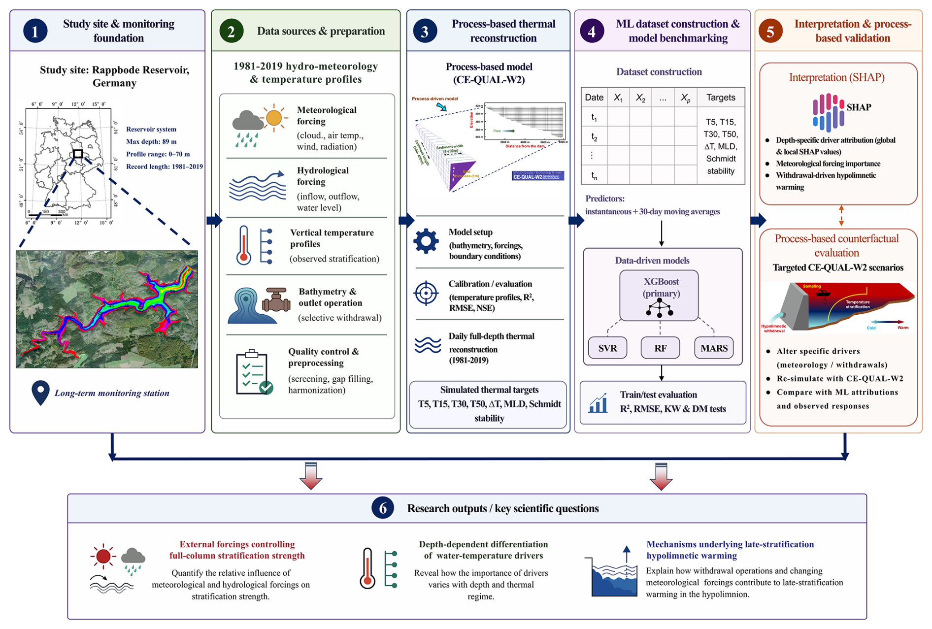
Figure 1 Study site and methodological workflow of the integrated CE-QUAL-W2 and machine-learning framework. The workflow links long-term monitoring and hydro-meteorological forcing with CE-QUAL-W2 thermal reconstruction, data-driven model benchmarking, SHAP-based attribution, and targeted process-based validation. The final outputs address stratification-strength controls, depth-dependent thermal drivers, and mechanisms of episodic hypolimnetic warming.

The reservoir is impounded within a narrow valley in the Harz Mountains. The regional catchment is underlain mainly by consolidated Paleozoic bedrock, including greywacke, clay schist, and diabase (Rinke et al., 2013; Werner et al., 2021). In the present hydrodynamic application, the model geometry and time-varying wetted domain are prescribed from reservoir bathymetry and observed water-level variations; subsurface geological sections are therefore not used to define the computational domain.

Inflows of the Rappbode Reservoir are delivered by the Hassel and Rappbode pre-reservoirs and by a transfer tunnel from the Königshütte Reservoir (Mi et al., 2018). Six selective-withdrawal outlets are embedded in the dam at 345, 360, 370, 380, 390, and 400 m a.s.l.; the lowest outlet discharges to the downstream Wendefurth Reservoir, whereas the 360 and 370 m intakes are routinely used for potable supply. With an annual residence time of roughly one year and the regional temperate climate, Rappbode exhibits a classic dimictic pattern: stable thermal stratification in summer and winter, and complete holomixis during spring and autumn. The national ban on phosphate-based detergents instituted three decades ago reduced total phosphorus from 0.16 mg L⁻¹ in 1990 to the current level of approximately 0.02 mg L⁻¹, and the reservoir is now classified as meso- to oligotrophic status (Mi et al., 2022).

2.2 Long-term water temperature measurements

Since 1981, bi-weekly vertical temperature profiles have been taken at the deepest point immediately upstream of the Rappbode Dam (see Fig. 1), spanning the full water column from the surface to 70 m depth. Up to 2008, temperatures at discrete depths were measured with a thermometer inside an open cylinder sampler; from 2009 onward, measurements have been acquired with a Hydrolab DS5 multiparameter probe. Parallel deployments during the transition period confirmed statistical equivalence between the two methods (Wentzky et al., 2018). In this study, we used data from 1981 to 2019 (39 years in total), and after quality control, the record yields a depth–time matrix with year-round, across-season coverage over the routine profiling range of 0–70 m, which serves as the basis for all subsequent analyses.

2.3 CE-QUAL-W2 model configuration

We developed an integrated framework linking four decades of water-temperature observations with process-based modeling and interpretable machine learning to elucidate the thermal evolution of the Rappbode Reservoir (Fig. 1). Here, the process-based simulations were performed with CE-QUAL-W2 (hereafter W2, version 4.2.1), a laterally averaged, two-dimensional hydrodynamic model originally developed by the U.S. Army Corps of Engineers at 1975 (Cole and Wells, 2006) and now maintained by the Department of Civil and Environmental Engineering at Portland State University. W2 is widely used as a standard tool for resolving hydrodynamic processes in lakes, reservoirs, and estuaries (e.g., Carr et al., 2019; Kobler et al., 2018).

For Rappbode, the computational mesh comprises four branches subdivided into 106 longitudinal segments (Δx= 100–400 m) and lateral sub-segments of 5–700 m, yielding 3876 grid cells with a uniform 1 m vertical resolution (Fig. S1 in the Supplement). This discretization fully resolves the reservoir's bathymetry, enabling precise simulation of its morphological features. Consistent with the W2 formulation, the main physical assumption in the present application is that lateral variations within each segment are secondary to longitudinal and vertical gradients; each segment is therefore represented by a laterally averaged cross-section. This assumption is appropriate for the narrow, dendritic morphology of Rappbode Reservoir and for the present objective of resolving open-water thermal stratification and withdrawal-induced vertical exchange. Groundwater exchange and subsurface hydrogeological flow were not explicitly represented. Thus, the depths shown in the model output and figures denote bathymetric water-column depths within the reservoir, rather than geological or hydrogeological sections. The model was driven by two sets of boundary conditions: (i) Hydrological forcing, including daily inflow discharge, inflow temperature, outflow discharge, and the withdrawal elevation at the dam, was provided by the Rappbode Reservoir authority (Talsperrenbetrieb Sachsen-Anhalt). The outflow boundary was prescribed directly from operator records, rather than inferred from the simulated thermal structure or adjusted during temperature calibration; (ii) meteorological forcing, including hourly air temperature, relative humidity, wind speed and direction, incoming short-wave radiation, and cloud cover, was obtained from a monitoring buoy moored near the reservoir's centre (Rinke et al., 2013), with gaps infilled with records from the German Weather Service station at Harzgerode, ∼ 15 km away from the reservoir. An intercomparison of Harzgerode and Rappbode Reservoir indicates a high degree of correlation in the meteorological records (see Mi et al., 2019 for more details). Simulations started on 1 January 1981 with an isothermal initial profile of 4 °C, representing a horizontally and vertically homogeneous state.

The present W2 application builds on earlier Rappbode Reservoir configurations (see Mi et al., 2020, 2023b), but all simulations reported here were re-run and evaluated for the 1981–2019 temperature archive used in this study. The model was calibrated manually using a trial-and-error procedure. Three site-specific parameters were adjusted because they depend on local optical conditions and meteorological exposure: the shading coefficient (SHADE), wind-sheltering coefficient (WSC), and pure-water light-extinction coefficient (EXH2O). The final values were SHADE = 1, WSC = 1, and EXH2O = 0.55 m⁻¹. All remaining parameters were retained at standard CE-QUAL-W2 settings because they are physically based and not typically subject to site calibration (Cole and Wells, 2006). The complete parameter set and numerical options are provided in Sect. S1 and Table S1. The main calibration targets were the temperatures at different depths, and water level was used as an additional system-scale check of the water-balance representation. To close the reservoir water balance, residual inflows required to match the observed water-level evolution were represented as distributed tributary inflows, following the water-balance procedure described in the official CE-QUAL-W2 User Manual (Wells, 2026). These residual inflows were used only for water-balance closure and were distributed along the main reservoir branch to minimize localized thermal effects. No separate split-sample validation period was defined. Instead, the full 1981–2019 observational record was used for continuous calibration and evaluation across a broad range of hydroclimatic and operational conditions. This choice follows the calibration guidance in the official manual of W2 (Wells, 2026), which emphasizes evaluating model behavior across broad observed conditions rather than relying on an arbitrary calibration/verification split.

2.4 XGBoost description and modeling framework

Data-driven approaches used in Earth-system prediction span a broad spectrum, including regression models, kernel methods such as Support Vector Regression, tree ensembles such as Random Forest and XGBoost, neural networks, and metaheuristic frameworks designed for optimization. Genetic algorithms and related metaheuristics are particularly valuable for search and optimization tasks, including parameter calibration, feature selection, and model structure exploration (Rajwar et al., 2023; Schiavo and Pedretti, 2026). The present study required a supervised regression model that could emulate CE-QUAL-W2 thermal targets from tabular hydrometeorological predictors and support transparent attribution across depths and stratification phases. We therefore selected XGBoost as the primary model because this tree ensemble framework is well suited to nonlinear tabular data, computationally efficient, and directly compatible with SHAP interpretation (Mi et al., 2024; Zhu et al., 2022). To place this choice in context, we further benchmarked XGBoost against three other data-driven approaches under the same experimental protocol.

2.4.1 XGBoost model description

Extreme Gradient Boosting (XGBoost) is an ensemble method that iteratively fits Classification-and -Regression Trees (CART) within a gradient-boosting framework. At each iteration t, the algorithm minimizes a regularized objective:

$$\begin{array}{}\text{(1)}& {\displaystyle }{L}^t={\sum }_{i=\mathrm{1}}^{n}l\left(y_i,{\widehat{y}}_i^{t-\mathrm{1}}+f_t\left(x_i\right)\right)+{\sum }_{k=\mathrm{1}}^t\mathrm{\Omega }\left(f_k\right)\text{(2)}& {\displaystyle }\mathrm{\Omega }\left(f\right)=\mathit{\gamma }T+{\displaystyle \frac{\mathrm{1}}{\mathrm{2}}}\mathit{\lambda }{\sum }_{j=\mathrm{1}}^T{w}_j^{\mathrm{2}}\end{array}$$

where l(⋅) is a twice-differentiable loss (squared error for regression), f_t is the tth tree, T is the number of leaves and w_j denotes leaf weights; γ and λ provide structural and weight regularization, respectively. Here, Ω(f) represents the regularization term that penalizes model complexity to prevent overfitting. By employing a second-order Taylor expansion of L^t, XGBoost obtains closed-form gain scores that guide an exact or histogram-based greedy search for the optimal split, while column subsampling and block-wise caching accelerate computation. This design yields three decisive benefits: (i) high accuracy, since second-order information markedly improves converge4nce; (ii) strong generalization, owing to L1/L2 shrinkage, learning-rate decay and stochastic sub-sampling; and (iii) computational efficiency, as multi-threaded and out-of-core execution scale to millions of observations and features on commodity hardware. Built-in cross-validation, early stopping and SHAP-based interpretability further underline XGBoost's suitability for handling small- to medium-sized and highly non-linear environmental data sets (Li et al., 2024; Lyu et al., 2019).

2.4.2 XGBoost model structure

We developed XGBoost models for predicting reservoir thermal structure according to daily outputs (1981–2019) from CE-QUAL-W2. Target variables comprise epilimnetic (5 m depth), metalimnetic (15 m depth), hypolimnetic (30 m depth) and bottom (50 m depth) temperatures, Schmidt Stability, the bottom-to-surface temperature difference and mixed-layer depth (see the Supplement for details on the last three indices and the post-processing methods). Since the above indices related to stratification dynamics are applicable only during thermal stratified period, therefore, the XGBoost model was constructed and analyzed exclusively for May–October. Guided by recent advances in machine-learning modeling of lentic thermal structures (e.g., Bertone et al., 2015; Kreakie et al., 2021), the predictor set includes both the instantaneous and 30 d moving-average values of observed air temperature, relative humidity, wind speed and direction, incoming short-wave radiation, cloud cover and reservoir outflow discharge. Descriptive statistics of the predictor and target variables used for machine-learning model development are summarized in Table S2. Here, we included 30 d moving-average predictors to represent the cumulative component of atmospheric and hydraulic influences across depths, with the physical basis for this setting (epilimnetic thermal inertia τ) further detailed in Sect. 4.2. To be noted, our previous studies indicated that inflow discharge exerted only a marginal influence on the reservoir's thermal structure (Mi et al., 2020); thus, it was excluded as an input feature from the XGBoost model. All predictors included in the analysis were linearly de-trended, Z-score standardized and screened for collinearity ($\left|\mathit{\rho }\right|\mathit{<}\mathrm{0.75}$) to minimize feature redundancy (Deka and Weiner, 2024).

The full machine-learning dataset was randomly split into training and testing subsets in an 80:20 ratio. Comparisons of the empirical cumulative distributions of the training and testing subsets, quantified by the Kolmogorov–Smirnov statistic together with Jensen–Shannon and energy distances, indicated no appreciable distributional shift for any target-specific model (Table S3). Within the training subset, a 5-fold rolling-origin cross-validation combined with Bayesian optimization was used to optimize the XGBoost hyperparameters (i.e., eta, max_depth, subsample, and colsample_bytree), and early stopping was applied to minimize the root mean square error (RMSE) on the validation folds. Model performance was then evaluated using RMSE and the coefficient of determination (R²), with training and testing results reported separately. The optimal values of eta, max_depth, subsample, and colsample_bytree were 0.2, 6, 0.7, and 0.7, respectively.

2.4.3 Other data-driven models for comparison

Comparative experiments were conducted to benchmark the predictive performance of XGBoost against three widely used data-driven models for reservoir thermal-structure prediction, including Support Vector Regression (SVR), Random Forest (RF), and Multivariate Adaptive Regression Splines (MARS). To ensure a rigorous and directly comparable benchmark, the three baseline models were trained and evaluated under an identical experimental protocol to XGBoost, covering predictors, train–test partitioning, and performance metrics. Statistical differences in predictive performance were evaluated by applying Kruskal–Wallis tests (Kruskal and Wallis, 1952) to the test-set squared-error distributions of XGBoost, SVR, RF, and MARS for each target variable, followed by pairwise Diebold–Mariano tests (Diebold and Mariano, 2002) comparing XGBoost with each benchmark model. All models were performed on a desktop workstation equipped with an Intel(R) Core(TM) Ultra 9 285K CPU @ 3.70 GHz, 256 GB RAM, and an NVIDIA T400 4 GB GPU.

SVR is a classical supervised regression algorithm developed within the support vector machine framework proposed by Cortes and Vapnik (Vapnik, 2013). The formulation follows the structural risk minimization (SRM) principle. The flexibility of SVR is provided by kernel functions, which transform nonlinear relationships in the original predictor space into linear representations in a higher-dimensional feature space. Here, the radial basis function (RBF) was used as the kernel function, with the regularization parameter C and ε-insensitive loss parameter set to 1 and 0.1, respectively.

RF is a tree-based ensemble learning framework (Yousefi and Toffolon, 2022). It constructs an ensemble of decorrelated decision trees by repeatedly drawing bootstrap samples from the training data and selecting random subsets of predictors at each split, and the final prediction is obtained by averaging the outputs of all trees. In this study, the model was configured with 500 decision trees, a minimum terminal node size of 50 samples, and bootstrap sampling with replacement for tree construction.

MARS is a nonparametric regression method that approximates covariate effects with adaptive piecewise linear splines. The fitted equation is built by forward addition of hinge pairs followed by backward pruning, thereby retaining nonlinear effects and predictor interactions in a parsimonious form (Heddam et al., 2020). In the present analysis, the maximum interaction degree was set to 2, the generalized cross validation penalty was 3, and the forward fitting threshold was 0.001.

2.4.4 SHAP-based feature contribution analysis

In the interpretability component of the modelling framework, we quantified feature contributions using SHapley Additive exPlanations (SHAP) values. SHAP is a model-agnostic interpretability framework rooted in cooperative game theory (Lundberg et al., 2020). It assigns each predictor a Shapley value calculated by evaluating the predictor's marginal contribution to model output across all possible subsets of input features (>0 pushes the prediction upward, <0 pulls it downward). We report the mean absolute SHAP for each feature as a measure of global importance. Here, SHAP distributions and effect sizes were visualized with beeswarm plots: the horizontal axis shows the SHAP value, and point color redundantly encodes the same measure on a single, shared scale (e.g., warm colors on the right indicate positive contributions, cool colors on the left indicate negative contributions, see Fig. 9). Feature attributions computed via SHAP satisfy exact additivity, local accuracy, and consistency (null-feature property), providing a rigorous quantitative basis for evaluating the relative contributions of hydrometeorological predictors on reservoir thermal dynamics. These SHAP values are interpreted here as statistical attributions to model predictions rather than as standalone evidence of physical causality. For more background on SHAP values, please refer to the Supplement (Sect. S2).

As complementary model-agnostic diagnostics, we further evaluated predictor relevance and response structure using permutation feature importance (PFI), partial dependence plots (PDPs), and individual conditional expectation (ICE) curves. PFI was calculated on the held-out test data by randomly permuting each predictor and quantifying the resulting increase in prediction error, following the permutation-based variable-importance framework introduced by Breiman (2001) and its model-agnostic formalization by Fisher et al. (2019). PDPs were used to summarize the average marginal response of hypolimnetic water temperature to dominant predictors, following Friedman (2001), whereas ICE curves were used to visualize observation-level heterogeneity in these fitted responses, following Goldstein et al. (2015). Together, PFI, PDPs, and ICE curves served as complementary model-agnostic diagnostics to the SHAP analysis, allowing predictor importance and observation-level response heterogeneity to be evaluated within a consistent interpretation framework.

3 Results

3.1 Model performance in simulating long-term reservoir hydrodynamics

The calibrated W2 accurately reproduced the interannual and seasonal water-level dynamics of Rappbode Reservoir over the 39-year period (R²=0.99, see Fig. S2), indicating that the hydrological boundary conditions and water-balance closure were implemented consistently. The water level typically attains its annual maximum in spring (April–May, ∼ 420 m a.s.l.) in response to increased rainfall, then declines sharply through summer driven by intensified evaporation and elevated drinking-water withdrawals. During winter, marked reductions in precipitation and inflows caused the water-level to continually decline, reaching annual minima at the end of the season (e.g., 395 m a.s.l. in 2002). All of these characteristic fluctuations were satisfactorily captured by the model.

The model successfully captured spatiotemporal dynamics of the reservoir's thermal structure (such as thermocline depth and stratification onset (offset), see Fig. 2). Simulated temperatures closely matched observations, with most points clustering along the 1:1 line (R²=0.95; RMSE = 0.97 °C, see Fig. 2b). The simulated mean temperature (6.61 °C) closely matched the observations (6.76 °C) over the study period. More specifically, the discrepancy between observed and simulated temperatures generally decreased with depth, as indicated by RMSE of 1.27, 1.31 0.75, and 0.59 °C at depths of 5, 15, 30, and 50 m, respectively (Fig. 3, Table S4). Both simulated and observed profiles show that the intra-annual temperature amplitude diminished sharply with depth: it exceeded 15 °C at 5 m depth, but declined to < 10 °C at 30 m and < 8 °C at 50 m (Fig. 3).

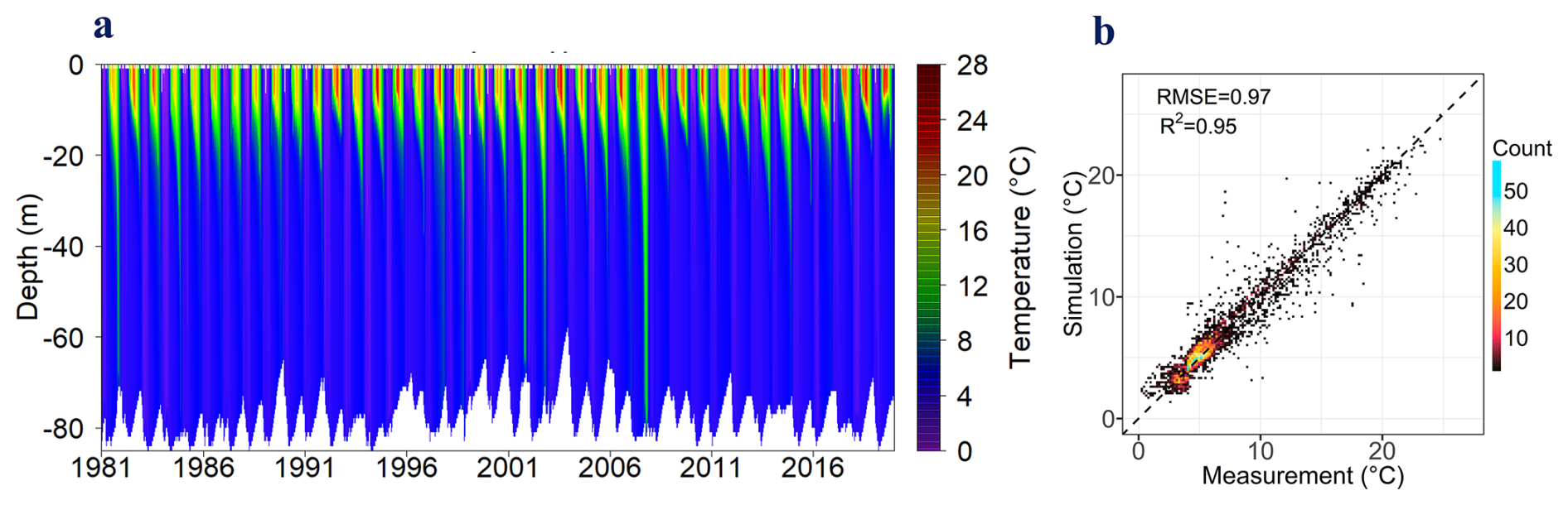
Figure 2 (a) Thermal dynamics of Rappbode Reservoir, from W2 simulation results, during the study period; (b) comparison between simulated and observed water temperature with the colour scale denoting the number of samples per hexagon. The dashed line represents the 1:1 line.

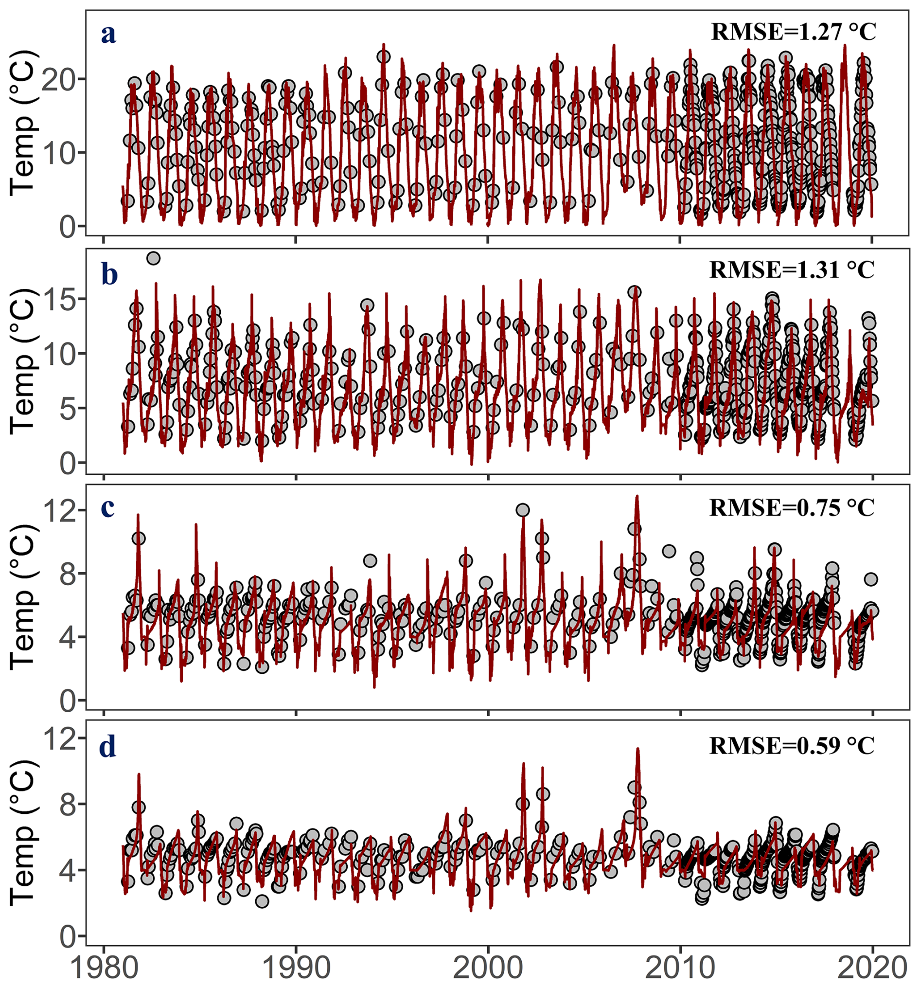
Figure 3 Observed (grey circles) versus simulated (black line) water temperatures in the Rappbode Reservoir at 5 (a), 15 (b), 30 (c), and 50 m (d). The RMSE for each panel is shown in the upper-right corner.

Additionally, we separated long-term monotonic trends from interannual variability using annual temperature series at representative depths (Fig. S3). At 5 m depth, both series warmed significantly, at rates of 0.05 K yr⁻¹ for the observations and 0.06 K yr⁻¹ for the simulations (Mann–Kendall test, p<0.05), with the mean epilimnetic temperature rising from ∼ 15 °C in 1981–1985 to ∼ 18 °C at the end of the record. By contrast, temperatures at 15–50 m exhibited pronounced year-to-year variability but no statistically significant monotonic trend (Mann–Kendall test, p>0.05). These depth-specific trends provide the long-term thermal context for the event-focused analysis of late-stratification bottom-water warming presented below.

3.2 Performance of XGBoost in simulating reservoir stratification dynamics

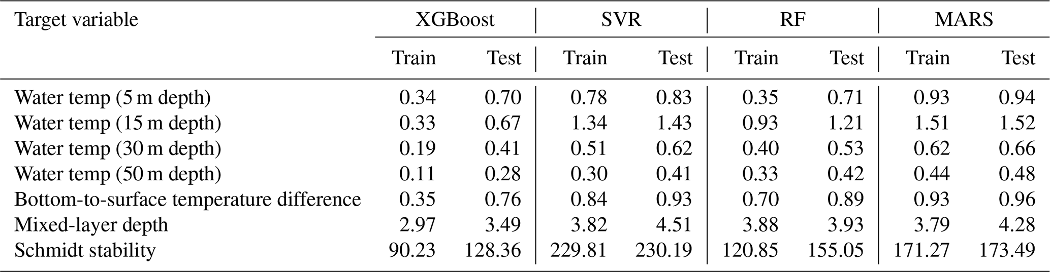
XGBoost consistently delivered the best point performance across all depth-specific temperature models, with the highest test R² and lowest test RMSE between W2 and XGBoost at all four depths (Table 1). Statistical tests further showed that its advantage over SVR and MARS was significant throughout, whereas the improvement over RF was significant at 15 and 50 m depth, but not at 5 or 30 m depth (Table S5). Using daily W2 outputs as targets, XGBoost exhibited progressively smaller prediction deviations with increasing depth, as RMSE between W2 and XGBoost declined from 0.70 °C at 5 m to 0.28 °C at 50 m. The seasonal temperature pattern was also accurately represented by XGBoost: surface temperatures (5 m depth) followed a pronounced unimodal, bell-shaped curve that peaked in mid-July to early August, when the median daily temperature in both W2 and XGBoost simulations was ∼ 19 °C, and cooled markedly at the onset (May) and offset (October) of the stratified period (Fig. 4). With increasing depth, the timing of peak temperature lagged progressively. At depths of 30 and 50 m, temperatures rose continuously throughout the stratified period, reaching their maxima in October.

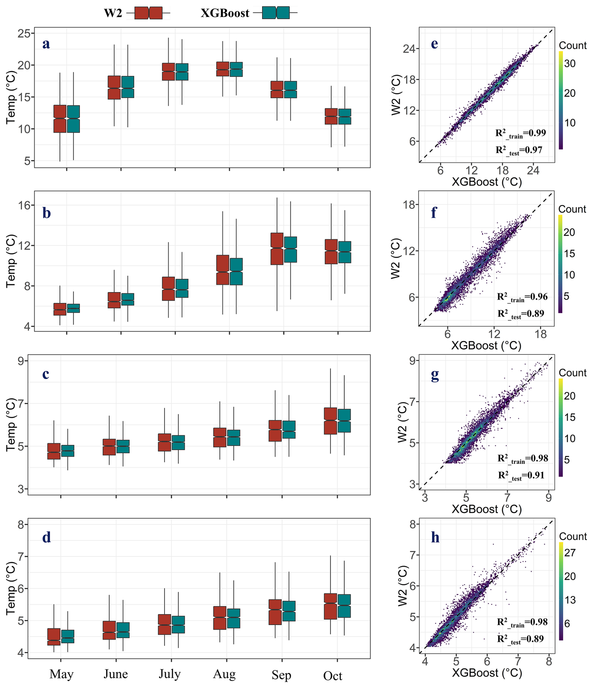
Figure 4 Water temperature simulated by W2 and XGBoost in Rappbode Reservoir at the depth of 5 (a), 15 (b), 30 (c) and 50 m (d), with the right column indicating the comparison for all specific depths. Training and testing R² values are reported separately in the corresponding panels.

XGBoost also outperformed the three benchmark models for the stratification metrics and reproduced the CE-QUAL-W2 outputs with close agreement (Fig. 5), yielding test R² values of 0.96, 0.82, and 0.97 and corresponding test RMSE values of 0.76 °C, 3.49 m, and 128.36 J m⁻² for bottom-to-surface temperature difference, mixed-layer depth, and Schmidt Stability, respectively (Tables 1 and 2). Specifically, Schmidt Stability was generally <1×10³ J m⁻² at the onset of stratification in May, increased steadily to a peak of $\sim \mathrm{3}\times {\mathrm{10}}^{\mathrm{3}}$ J m⁻² in August, and declined thereafter, returning to the initial levels by October; this seasonal pattern closely paralleled that of the bottom-to-surface temperature difference (Fig. 5a). In contrast, the mixed-layer depth deepened throughout the stratified period: it remained < 10 m from May to August but reached approximately 20 m by October (Fig. 5b).

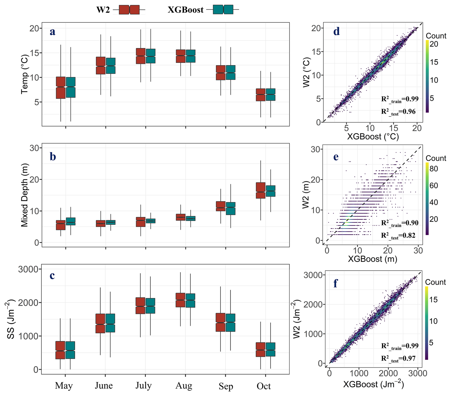
Figure 5 Stratification dynamics simulated by W2 and XGBoost in Rappbode Reservoir for bottom-to-surface temperature difference (a), mixed-layer depth (b) and Schmidt Stability (c), with the right column indicating the comparison for the three indexes. Training and testing R² values are reported separately in the corresponding panels.

Table 1 Benchmark comparison of data-driven model performance in reproducing CE-QUAL-W2-simulated reservoir thermal-structure variables. Coefficients of determination (R²) are reported separately for the training and testing datasets across all target variables, including depth-specific water temperatures and stratification metrics, for XGBoost, SVR, RF, and MARS.

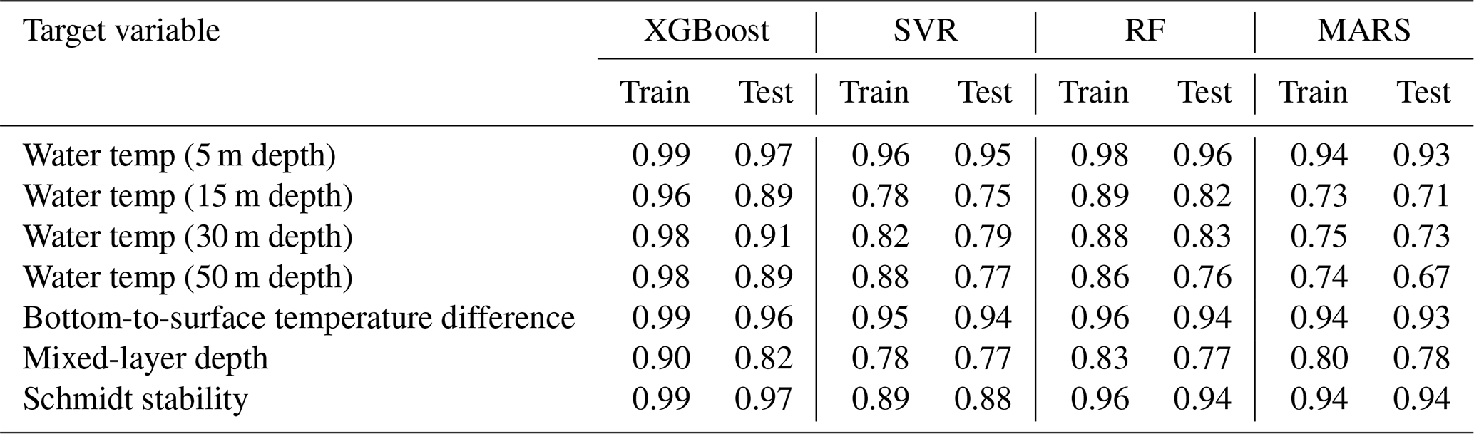
Table 2 Benchmark comparison of data-driven model performance in reproducing CE-QUAL-W2-simulated reservoir thermal-structure variables based on root mean square error (RMSE). RMSE values are reported separately for the training and testing datasets across all target variables, including depth-specific water temperatures and stratification metrics, for XGBoost, SVR, RF, and MARS. RMSE is expressed in °C for water temperature, m for mixed-layer depth, and J m⁻² for Schmidt Stability.

Because XGBoost consistently outperformed the three benchmark models across all temperature and stratification targets, it was used as the reference model for subsequent SHAP-based interpretation of driver importance. SHAP analysis of the XGBoost model indicates that epilimnetic temperature (5 m) is governed chiefly by the antecedent 30 d means of air temperature, dew-point temperature, and incident short-wave radiation (Fig. 6). With depth, the relative SHAP contribution of air temperature decreases, ranking third, fourth, and fifth for the temperature at 15, 30, and 50 m depth, respectively, while short-wave radiation becomes the primary external driver below the surface layer. The importance of outflow discharge strengthens progressively down-profile, ranking eighth for epilimnetic temperature, fourth for temperature at 15 m depth, and second for temperature at 50 m depth. The relative importance of cloud cover as a driver of water temperature increased incrementally with depth, ranking sixth at depths of 5–30 m and fourth at 50 m. Wind speed and direction remain comparatively minor controls across all depths, ranking between sixth and eighth (Fig. 6). In sum, SHAP resolves a depth-structured forcing pattern: atmospheric control shifts from non-radiative terms in the epilimnion to short-wave radiation below the surface layer, while hydraulic withdrawal gains influence toward the hypolimnion. Complementary PFI analyses reproduced this vertical ordering of dominant controls (Fig. S4): antecedent air temperature ranked first at 5 m, whereas antecedent shortwave radiation dominated at 15 and 30 m and outflow discharge increased in importance with depth.

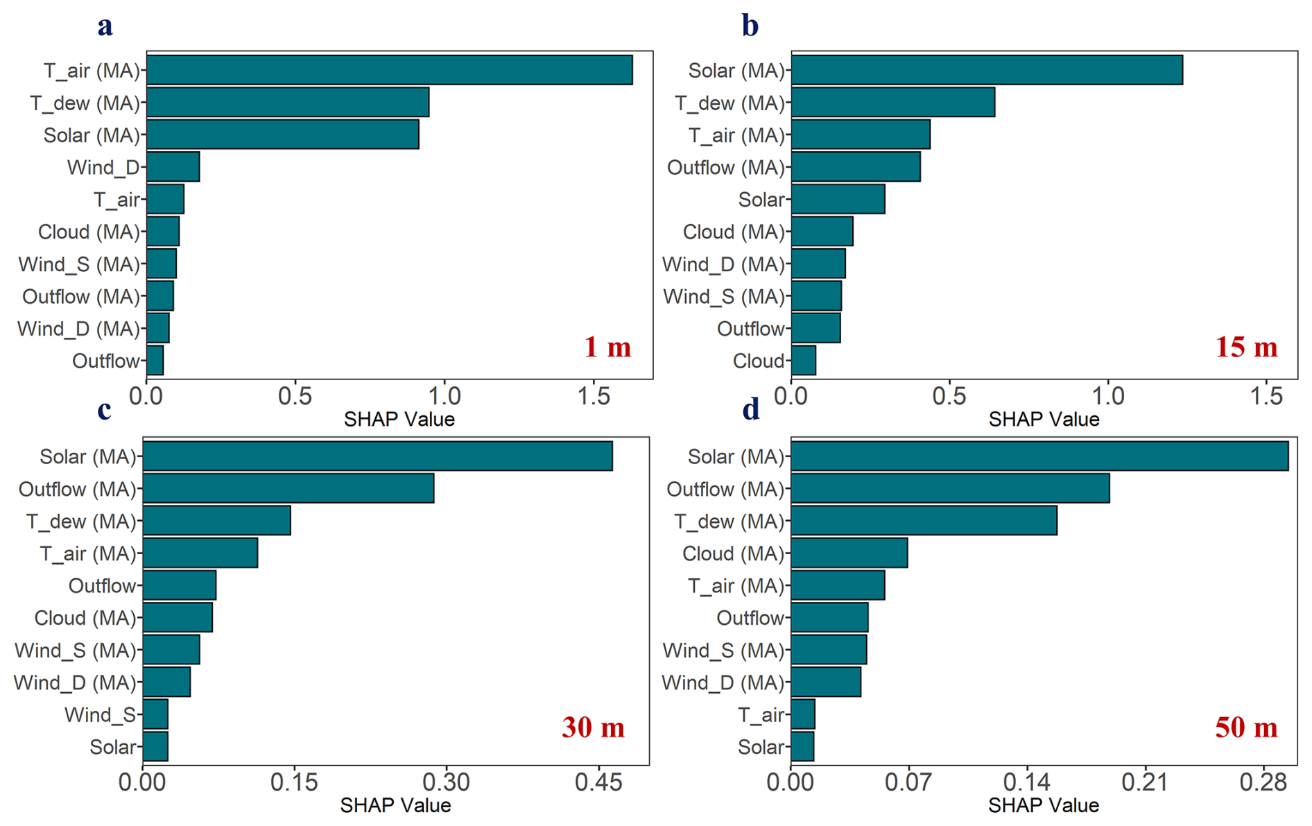
Figure 6 Driving factors analysis for water temperature at the depth of 5 (a), 15 (b), 30 (c) and 50 m (d) based on the SHAP values. MA indicates moving-average features.

Our results also indicated that both the bottom-to-surface temperature difference and Schmidt Stability are governed principally by the antecedent 30 d means of air temperature, incident short-wave radiation, and dew-point temperature (Fig. 7). By comparison, the mixed-layer depth was primarily driven by short-wave radiation over the preceding 30 d period, with outflow discharge and dew-point temperature ranking second and third, respectively. Cloud cover also significantly affected stratification dynamics, ranking fourth in importance for mixed-layer depth and fifth for Schmidt stability. In addition to antecedent forcings, instantaneous (same-day) conditions also exerted substantial control: specifically, same-day air temperature ranks fourth for its effect on both the bottom-to-surface temperature difference and Schmidt Stability (Fig. 7), whereas the same-day outflow discharge ranks fifth in modulating mixed-layer depth.

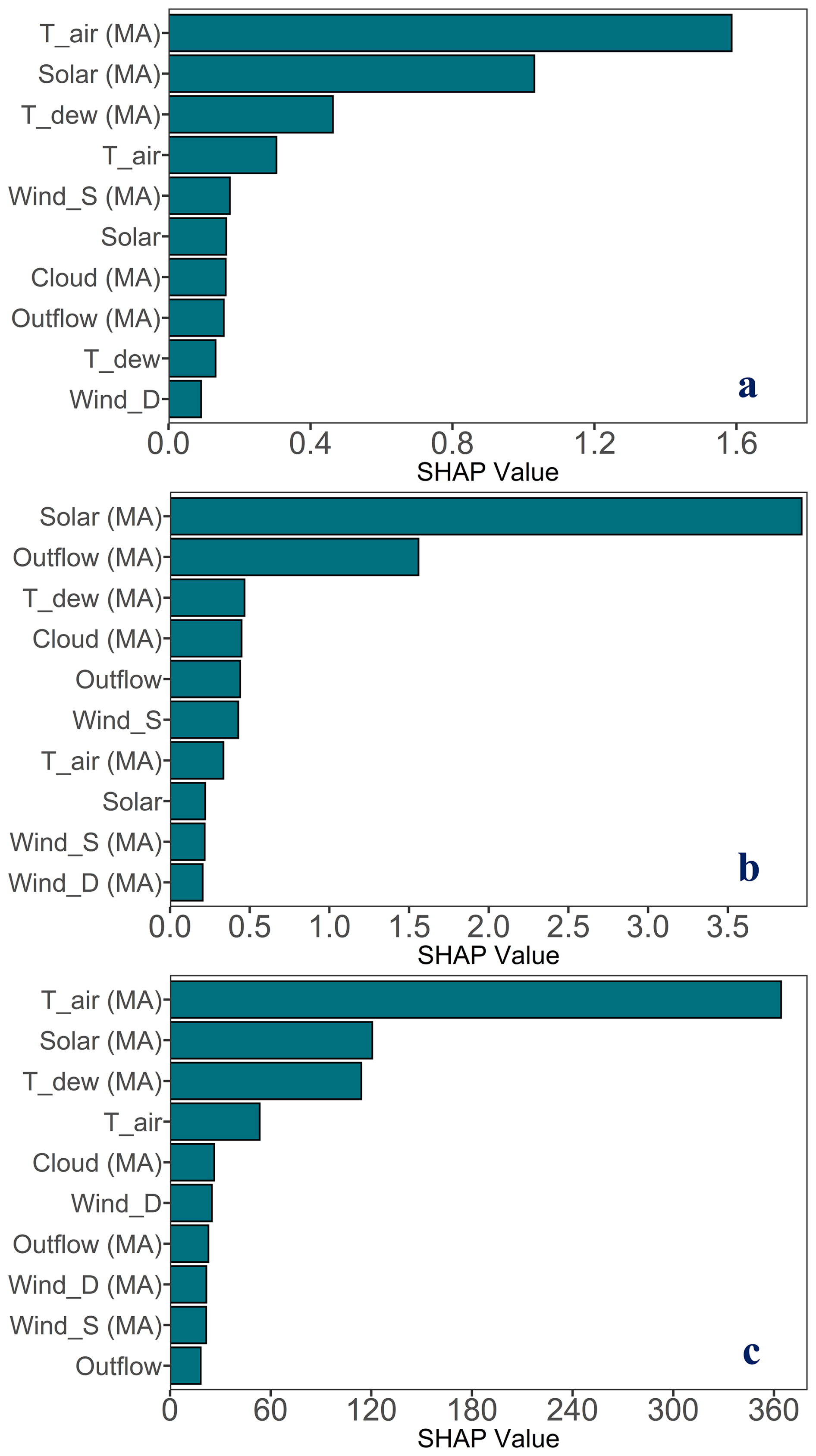
Figure 7 Driving factors analysis for bottom-to-surface temperature difference (a), mixed-layer depth (b) and Schmidt Stability (c), based on the SHAP values. MA indicates moving-average features.

3.3 Mechanisms underlying the occurrence of elevated bottom-water temperatures in specific years

During the stratified season, hypolimnetic (50 m depth) temperatures in Rappbode Reservoir generally remains within the range of 4–6 °C. However, both in-situ profiles and W2 simulations reveal episodic warming to ∼ 10 °C at the end of stratification (September–October) in 1981, 2001, 2002, and 2007 (Fig. 8b). These years were therefore treated as episodic departures within a deep-water temperature record that showed strong interannual variability but no significant monotonic trend. To elucidate the mechanisms underlying these anomalies, daily hypolimnetic temperatures simulated by W2 were adopted as targets to develop specific XGBoost models for early (May–June), mid (July–August), and late (September–October) stratified periods. SHAP analysis was then applied to quantify the dominant predictors in each interval.

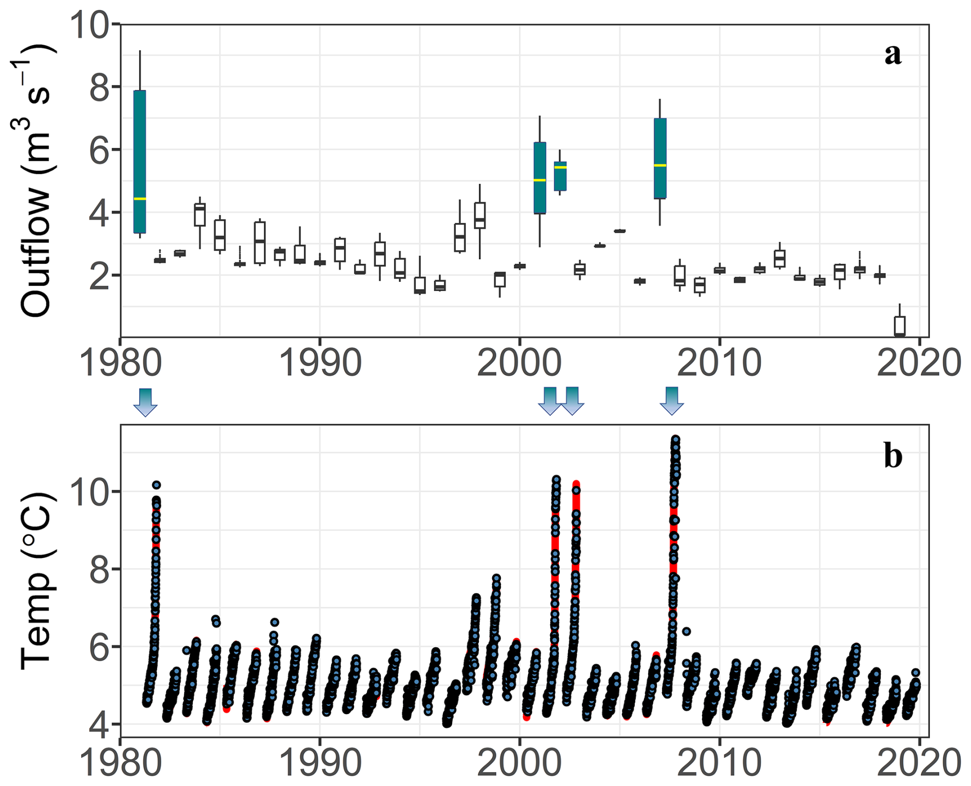
Figure 8 (a) Moving-average of discharge during September–October for each year (with 1981, 2001, 2002, and 2007 highlighted in green); (b) water temperature, at the depth of 50 m, from W2 (red lines) and XGBoost (black point) for each year.

The period-specific XGBoost models satisfactorily reproduced CE-QUAL-W2 hypolimnetic temperatures with RMSE of 0.08, 0.09 and 0.13 °C for early, mid and late stratification, respectively (R²= 0.96–0.98). The results further demonstrate pronounced stage-dependent shifts in the controls on hypolimnetic temperature (Fig. 9). Specifically, during the early-stratified period (May–June) the 30 d antecedent mean air temperature, outflow discharge and wind direction emerge as the three leading drivers. By mid-stratification (July–August) the principal controls change over to the 30 d mean short-wave irradiance followed by outflow discharge, whereas in the late-stratified phase (September–October) the positive influence of outflow discharge becomes overwhelmingly dominant (Fig. 9): its SHAP contribution attains 0.513, over four times greater than that of air temperature (0.131, ranked second) and shortwave radiation (0.115, ranked third). To corroborate this finding, we examined years in which late-season hypolimnetic temperatures were anomalously elevated. In 1981, 2001, 2002, and 2007, the median discharge during late stratification was 5.24 m³ s⁻¹, approximately 125 % higher than the 40-year median (2.32 m³ s⁻¹) for this interval, a difference that was statistically significant (Dunn's test, p<0.05, see Fig. 8a). Furthermore, during this period, the SHAP contribution of outflow discharge was also markedly greater than those of the other predictors (Fig. 9d). Complementary explainability analyses supported this interpretation (Figs. S4–S5). PFI again identified antecedent outflow as the dominant predictor of late-stratification bottom-water temperature. PDP and ICE curves likewise showed a strong positive and nonlinear warming response to increasing antecedent outflow, while antecedent air temperature and antecedent shortwave radiation exerted weaker and more heterogeneous effects. Local SHAP decompositions for two representative late-stratification cases further highlight this event-scale contrast (Fig. S6). In the strongest anomalous warming case (2 October 2007), antecedent outflow discharge increased the model-predicted 50 m water temperature by > 3 °C, whereas antecedent air temperature, cloud cover, and shortwave radiation each contributed < 0.5 °C. By contrast, the reference case was defined as the non-anomalous late-stratification day whose bottom-water temperature was closest to the median of all non-anomalous late-stratification cases (11 September 1988); on that day, no comparable positive outflow-discharge contribution was detected, and all feature-level contributions remained small ($\left|\mathrm{SHAP}\right|\mathit{<}\mathrm{0.12}$ °C). Collectively, the hydrological signature provides independent evidence that enhanced release discharge is the key driver of late-stratification hypolimnetic warming.

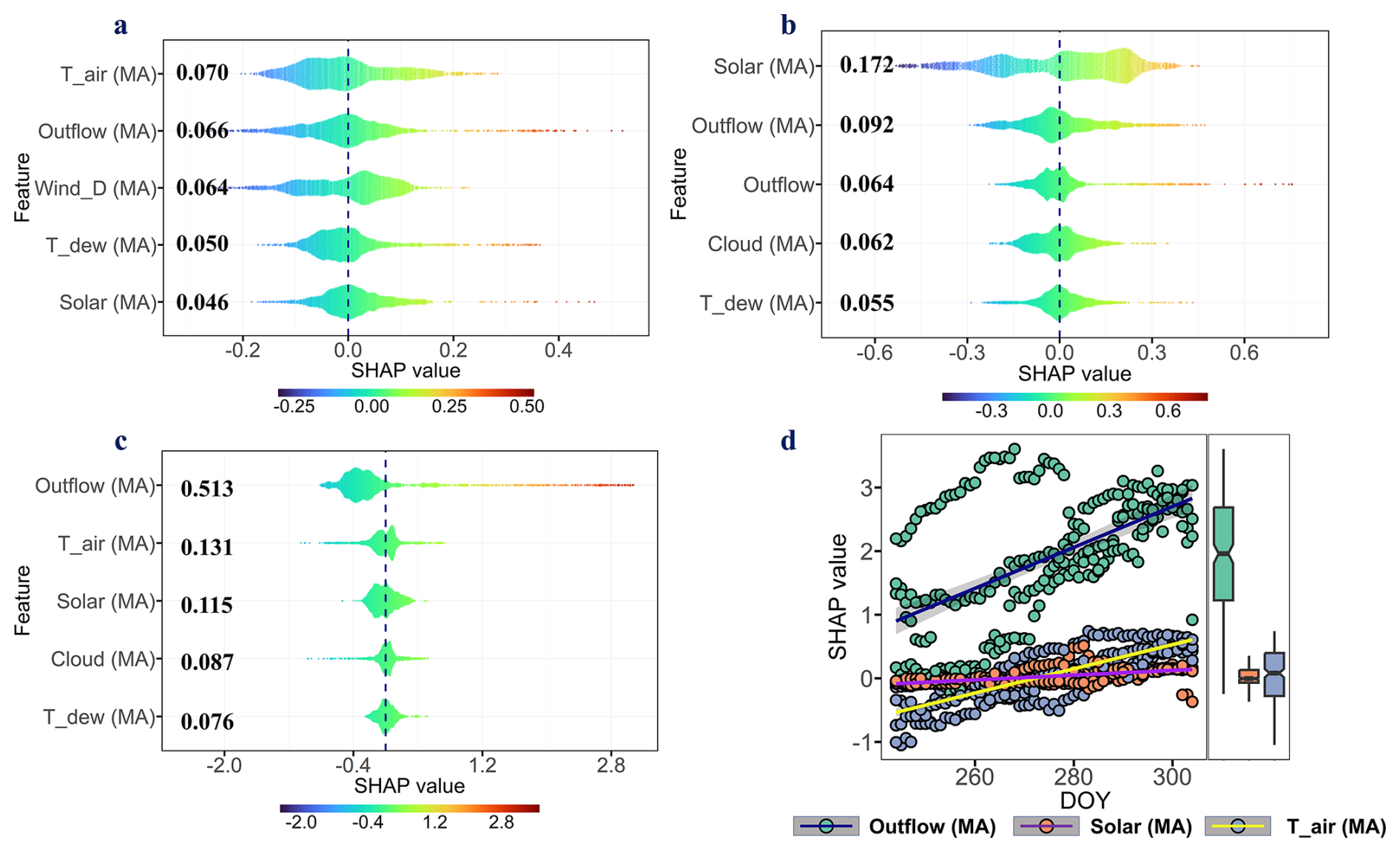
Figure 9 Comparison of SHAP-derived driver importance for bottom-layer water temperature at 50 m depth. (a)–(c) SHAP value rankings showing how dominant drivers vary across the initial (May–June), middle (July–August), and final (September–October) stages of stratification. (d) Comparison of SHAP values during September–October for outflow (green), solar radiation (red), and air temperature (blue) in 1981, 2001, 2002, and 2007; points denote daily values plotted against day of year (DOY), with colored lines indicating linear regression fits, and adjacent boxplots summarizing the corresponding distributions. MA indicates moving-average features.

4 Discussion

4.1 Reconstruction of thermal structure from multi-decadal full-profile observations

In this study we assembled a uniquely long and vertically resolved data set comprising almost four decades (1981–2019) of temperature profiles (0–70 m) and concomitant meteorological forcing for Rappbode Reservoir, the largest drinking water reservoir in Germany. On this basis, we established an analytical framework, combining process-based (CE-QUAL-W2) and data-driven (XGBoost) models, to systematically assess their capabilities in reproducing the reservoir's thermal structure. Whereas most publicly available lake- and reservoir-temperature records span ≤ 10 years and provide limited long-term coverage of deep-water temperatures (Ladwig et al., 2021; Woolway et al., 2020), the 39-year full-profile archive assembled here offers a robust empirical basis for multi-decadal hydrodynamic modelling.

Here, the long-term observations and simulations consistently indicate a pronounced epilimnetic warming of the reservoir, with observed and simulated warming rates of 0.06 and 0.05 °C a⁻¹, respectively. These rates are comparable to, and slightly higher than, the concurrent regional air-temperature trend (0.04 °C yr⁻¹; Mann–Kendall test, p=0.001), and are broadly consistent with warming rates reported for temperate lakes in previous large-scale syntheses (O'Reilly et al., 2015; Shatwell et al., 2019). In contrast, deep-water temperatures at 30 and 50 m depth exhibited no significant trends, thereby reflecting a characteristic pattern of intensified surface warming concurrent with relatively stable deep-water temperatures. This non-monotonic deep-water background is important for interpreting the anomalously warm late-stratification years analyzed below: these events represent episodic departures from long-term variability rather than evidence of sustained hypolimnetic warming over the full record.

This vertical asymmetry in warming preserves the cold-water refuge but implies a strengthening of thermal stratification. Numerous studies have shown that such shifts in lake and reservoir thermodynamics would exacerbate hypolimnetic anoxia and enhance internal nitrogen and phosphorus loading (Sun et al., 2022; Weinke and Biddanda, 2019), subsequently impairing source-water quality and downstream aquatic ecosystems (Jane et al., 2023). Accordingly, coupling the validated thermal models with biogeochemical modules to quantify present-day and future trajectories of dissolved oxygen, and to develop targeted water-quality management strategies, constitutes a logical and necessary extension of the current work.

4.2 Atmospheric and hydraulic drivers governing thermal dynamics in stratified reservoirs

The SHAP values indicated that the antecedent 30 d mean air temperature is the most influential predictor of epilimnetic temperature, as well as of Schmidt stability and the bottom-to-surface temperature difference, followed by dew-point temperature and shortwave radiation. This hierarchy corroborates earlier findings derived from short-term datasets for dimictic lakes by Livingstone and Lotter (1998) and Darko et al. (2019), and is now quantitatively confirmed by our 39-year observational record. All such results highlight the lagged response of the three surface-heat-forced stratification metrics to cumulative antecedent heat fluxes (i.e., the thermal inertia effect). Here, the epilimnetic thermal inertia was estimated from a mixed-layer heat budget. The areal heat capacity of the mixed layer is ρc_ph, where ρ is water density, c_p is the specific heat capacity of water (4.18×10³ J kg⁻¹ K⁻¹), and h is mixed-layer depth. The characteristic timescale of a 1 K mixed-layer temperature response under a mean net heat flux H_net can therefore be estimated as:

$$\begin{array}{}\text{(3)}& {\mathit{\tau }}_{\mathrm{1}\mathrm{K}}={\displaystyle \frac{\mathit{\rho }{c}_{p}h\mathrm{\Delta }T}{\mathrm{|}{H}_{\mathrm{net}}\mathrm{|}}},\mathrm{\Delta }T=\mathrm{1}\mathrm{K}\end{array}$$

This estimate follows the same physical basis as the lake temperature formulation of Piccolroaz et al. (2013). For Rappbode Reservoir, using ρ=998 kg m⁻³, h= 9–11 m, and H_net= 18–24 W m⁻² for the stratified period (Mi et al., 2019) gives a characteristic response time on the order of several weeks, consistent with the 30 d averaging window that dominates the SHAP ranking. Because this response time exceeds the characteristic 1 d scale of surface heat-flux variability by an order of magnitude, daily atmospheric perturbations are strongly filtered by thermal inertia and thus contribute little to the statistical ranking.

By comparison, in the hypolimnion (30–50 m), short-wave radiation exceeds air temperature in the SHAP ranking, and the importance of outflow discharge concurrently increases, because sustained deep withdrawals can remove the coldest layers, erode thermocline stability and induce compensation flows that advect warmer water downward (Olsson, 2021; Weber et al., 2017), thereby regulating hypolimnetic temperature. Our analysis further reveals that, for mixed-layer depth, outflow discharge emerges as the second-most influential predictor. As shown above, this can be attributed to sustained hypolimnetic withdrawals, which induce downward flows and consequently deepen the mixed layer (Deng et al., 2011; Mi et al., 2023a). Additionally, the role of cloud cover should not be overlooked (ranking fourth in SHAP values), since cloudiness can effectively modulate incoming shortwave and longwave radiation, thus altering surface buoyancy fluxes (Boehrer and Schultze, 2008).

We further tested this SHAP-derived meteorological ranking using four targeted CE-QUAL-W2 scenarios in which shortwave radiation, air temperature, dew-point temperature, or cloud cover was separately replaced by its long-term median for the same calendar day during 1 April to 31 October, with all other forcings unchanged. Details of the scenario design and diagnostic calculation are provided in Sect. S4.1. The scenario results reproduced the key SHAP pattern: air temperature remained the strongest meteorological forcing for the water temperature at 5 m depth, whereas shortwave radiation ranked highest at the other subsurface layers. This agreement strengthens the physical credibility of the SHAP result that antecedent shortwave radiation has the highest relative contribution to thermal variability at greater water-column depths.

4.3 Late-season hypolimnetic warming – process interpretation of period-specific SHAP signals

During late stratification, increased deep-layer withdrawals are more effective at warming the hypolimnion because the reservoir is already in a mechanically vulnerable stratification state. Over this period, nocturnal cooling and declining net radiation substantially reduce Schmidt stability to <1×10³ J m⁻² (Fig. 5), compared with >2×10³ J m⁻² in midsummer (July–August). This weaker density structure lowers the buoyancy resistance across the metalimnion, allowing bottom-withdrawal forcing to enhance entrainment and compensatory downward transport of warmer upper-layer water. In parallel, the mixed layer deepens from about 6 m in early summer to 18 m by September–October (Fig. S8), thereby reducing the vertical distance between the mixed-layer base and the water-withdrawal intake (at the depths of 60–70 m) by ≈20 %. Over the same period, hypsographic calculations combining the W2 volume–elevation curve, daily water level, and mixed-layer depth indicated that the mean water volume below the mixed-layer base decreased from 8.78×10⁷ to 4.67×10⁷ m³, corresponding to a 46.8 % reduction. Thus, a given bottom-withdrawal discharge acted on a substantially smaller deep-water volume during late stratification, increasing the withdrawal-to-volume ratio and allowing the density interface to be displaced more efficiently. The concurrence of a weakened stratification intensity, reduced deep-water volume and a contracted transport pathway provides a physical basis for why high-discharge deep withdrawals can rapidly elevate bottom temperatures during late stratification. We further tested this interpretation using targeted CE-QUAL-W2 withdrawal scenarios for the four anomalous years. In the P50 and P90 scenarios, bottom withdrawal during 1 August to 31 October in 1981, 2001, 2002 and 2007 was replaced by the median and 90th percentile, respectively, of the corresponding calendar day values from the non-anomalous years. The thermal response was evaluated for September to October, when anomalous bottom warming occurred. The results suggested that reducing high bottom withdrawals strongly suppressed hypolimnetic warming: the mean 50 m temperature across the four anomalous years decreased from 8.05 in the baseline simulation to 6.30 in P90 and 6.00 °C in P50, while the corresponding maximum temperature decreased from 11.37 to 8.43 and 6.99 °C. These scenarios provide support for the interpretation that intensified bottom withdrawals contributed to hypolimnetic warming, consistent with the SHAP-derived dominance of outflow discharge during late stratification. Details of the scenario design and results are provided in Sect. S4.2.

Despite pronounced hypolimnetic warming induced by deep-water withdrawals in the late stratification periods of 1981, 2001, 2002, and 2007, the surface-to-bottom temperature difference remained above 1 °C for most of October (Fig. S9), indicating persistent and stable stratification conditions (Fang and Stefan, 2009). Hypolimnetic warming under such weakened stratification poses a severe ecological threat since oxygen demand in the hypolimnion increases sharply with temperature while atmospheric re-oxygenation remains inhibited. For Rappbode Reservoir, our previous work suggested that raising bottom-water temperature from a typical 6 to 10 °C (October 2001) augments the sediment oxygen demand (SOD) from 0.46 to 1.04 g O2 m⁻² d⁻¹ (Mi et al., 2020). Under a persistent density barrier, this additional demand cannot be offset by oxygen replenishment from surface waters, greatly amplifying the risk of hypolimnetic anoxia. Such adverse effects associated with a “warm yet stratified” state have also been systemically documented at the CW Bill Young Regional Reservoir (Bryant et al., 2024), and Cedar Lake (James et al., 2015), USA. Taken together, these observations underscore the management relevance of hypolimnetic warming during late-season stratification decay; accordingly, future work should quantify threshold conditions that link this warming to hypolimnetic oxygen debt, for example through stability and withdrawal-rate percentiles, and test operational adaptation strategies that minimize exposure to this state.

4.4 An integrated analytical framework for long-term thermal reconstruction and driver attribution

Our study not only clarifies the thermal dynamics of reservoirs and their external drivers, but also introduces a new methodology that is of broader interest. By integrating routine observations with calibrated and evaluated CE-QUAL-W2 hindcast simulations for Rappbode Reservoir, we reconstruct a four-decade, depth-resolved (0–70 m) temperature archive with high vertical and temporal resolution, transforming sparse monitoring into continuous vertical profiles for subsequent analyses. Second, an interpretable machine-learning workflow (XGBoost with rolling-origin cross-validation and early stopping) provides fast, accurate prediction across depths, which is directly relevant for forecasting use-cases increasingly requested by reservoir managers (Carey et al., 2022). Third, the SHAP analysis provides additive, model-consistent statistical attributions that decompose thermal anomaly into depth- and sample-specific contributions of individual predictors. In practice, this yields a quantitative explanation of reservoir thermal anomalies without running time-consuming large scenario ensembles with the process model. Collectively, these advantages constitute an integrated mechanistic–statistical framework that is readily transferable to other stratified lakes and reservoirs for long-term thermal reconstruction, driver attribution and operational evaluation.

When this framework is extended beyond a single monitoring station, geostatistical approaches become particularly relevant because spatial covariance and interpolation are then central to the analysis. Methods such as kriging, co-kriging, and hybrid geostatistical–machine-learning frameworks can be highly effective for spatial covariance modelling, interpolation among monitoring sites, and prediction at unsampled locations (Brcković et al., 2025; Grey et al., 2025). These methods were not implemented here because the present analysis focused on depth-resolved temporal attribution at a fixed reservoir station, using a physically consistent CE-QUAL-W2 reconstruction rather than spatial interpolation across monitoring locations. They would be particularly valuable in future applications that extend this framework to multi-station observations or reservoir networks, where spatial covariance and temporal driver attribution need to be evaluated jointly.

5 Conclusion

We developed an integrated CE-QUAL-W2 and machine-learning framework that reliably reconstructs, over nearly four decades, the full-depth thermal structure of Rappbode Reservoir, capturing the spatiotemporal variability of layer-specific temperatures and stratification-strength metrics.

SHAP attribution based on the integrated framework indicated strong vertical heterogeneity in the predictors of reservoir thermodynamics: surface temperature was primarily associated with the antecedent 30 d means of air temperature, dew-point temperature, and incident shortwave radiation, whereas the influence of shortwave radiation and outflow discharge increased progressively with depth and the relative effect of air temperature strongly declined.

The dominant predictors of bottom-water temperature shifted systematically across stratification phases: during early stratification (May–June), the leading drivers were the antecedent 30 d mean air temperature, outflow discharge, and wind direction; during mid stratification (July–August), shortwave radiation and outflow discharge jointly dominated; during late stratification (September–October), outflow discharge became the largest contributor, with a SHAP contribution more than four times that of air temperature and shortwave radiation.

Observations and simulations consistently showed that bottom-water temperature rose anomalously to ∼ 10 °C during late stratification in 1981, 2001, 2002, and 2007, whereas it typically remained at 4–6 °C in other years. Further analyses indicated that these events were largely linked to intensified deep withdrawals in late stratification, with outflow discharge ∼ 2.25 times higher than in typical years. The enhanced discharge weakened the density gradient and strengthened downward compensatory transport, driving the bottom-water thermal anomaly.