Influence of rainfall event characteristics and antecedent conditions on subsurface stormflow response of two forested hillslopes

Subsurface stormflow (SSF) is a critical runoff-producing mechanism in many upland and mountainous environments, yet the complex relationships between antecedent conditions, rainfall characteristics and SSF response are still not fully understood. Worldwide, the small number of SSF collection systems (trenches), as well as the generally small number of investigated SSF events limit our ability to generalize the findings and explore the influence of a broader range of storm sizes, intensities, antecedent wetness conditions and different hydrogeologic settings. In this study, we present a comprehensive analysis of SSF event characteristics in combination with rainfall event characteristics (depth and intensity), and antecedent conditions. The analysis is based on data collected over a 2-year period at two forested hillslope sites. Our results show that SSF volume is primarily controlled by total rainfall (P_tot) and antecedent wetness, with volumes being up to three orders of magnitude larger under wet initial conditions. The peak SSF flow rates of smaller events were correlated with P_tot and antecedent conditions, but for larger events (P_tot>ca. 20 mm), rainfall intensity and rainfall amount preceding peak rainfall intensity were more influential predictors than antecedent conditions. The steepness of the rising limb of the SSF hydrograph was correlated with P_tot and rainfall intensity. The antecedent soil moisture index (ASI) together with P_tot showed a high correlation with most SSF characteristics. The seasonal analysis revealed that, statistically, the largest SSF volumes occurred in winter and spring, while the highest peak flows were observed in spring and summer. Our results highlight the complex interactions among SSF responses, rainfall characteristics, and antecedent wetness conditions, underscoring the value of long-term monitoring across different seasons.

1 Introduction

Subsurface stormflow (SSF) is a key runoff-producing mechanism in many natural landscapes, often contributing significantly to the storm hydrograph of streams (McGuire et al., 2024; Peters et al., 1995; Weiler et al., 2006). Therefore, understanding the controls and processes governing SSF is essential for the future development of more robust rainfall-runoff models, particularly in light of increasingly extreme climatic conditions (Kirchner, 2006; Tabari, 2020; Weiler and McDonnell, 2007).

Subsurface flow contributing to storm runoff (i.e. SSF) typically develops when percolating water encounters a downslope-dipping horizon or interface with reduced saturated hydraulic conductivity that limits vertical drainage; when the downward flow exceeds the percolation capacity across this horizon/interface, water perches and is diverted laterally towards the stream (Weiler et al., 2006). Alternatively, SSF can be generated through the “transmissivity feedback mechanism”, in which the rise of the water table into a more permeable zone induces a faster, lateral, stream-reaching flow (Bishop et al., 1990; Weiler and McDonnell, 2004). The quick subsurface flow response to rainfall can be coupled to high flow velocities along preferred pathways (preferential flow) as well as to the rapid increase of a more diffuse flow (matrix flow) (Blume and van Meerveld, 2015; Weiler et al., 2006). Preferential SSF occurs when water flows along larger interconnected voids in the matrix (e.g. soil pipes or fractures), through matrix zones characterized by a higher permeability than their surroundings, or in a channelized fashion dictated by the irregular topography of an impeding layer (Anderson et al., 2009; Weiler et al., 2006).

Several factors govern SSF generation, including the characteristics of the macropore and fracture networks, the spatial variation in soil thickness, the topography of surface and impeding layer (i.e. depression storage) and the vertical variation in hydraulic conductivity, which controls the vertical percolation, leakage rate through the impeding layer and the possible onset of faster lateral flow within upper more permeable layers (Hopp and McDonnell, 2009; McGuire et al., 2024). Antecedent wetness conditions further modulate the SSF responses. Wetter soils promote SSF, as they require less additional rainfall to reach saturated or close-to-saturated conditions and initiate lateral flow (Guo et al., 2014; Penna et al., 2011; Uchida et al., 2005). Nevertheless, dry conditions can lead to the formation of soil cracks and support hydrophobicity of soils, both favouring preferential SSF (Buttle and Turcotte, 1999; Peters and Ratcliffe, 1998; Tromp-van Meerveld and McDonnell, 2006a). Rainfall characteristics – including total depth, intensity, and temporal distribution – also play a crucial role. Greater rainfall amounts increase the overall water content and hydraulic head, promoting the connectivity of saturated areas across the hillslope, which enhances SSF generation (Hopp and McDonnell, 2009; Tromp-van Meerveld and McDonnell, 2006b). Hence, the contributing area expands with increasing rainfall amounts, leading to a more uniform hillslope response (Hrnčíř et al., 2010; Šanda and Císlerová, 2009; Tromp-van Meerveld and McDonnell, 2006b).

The relationship between total event rainfall and resulting SSF volume is often nonlinear, with threshold-like behaviour observed in many studies (Tromp-van Meerveld and McDonnell, 2006a; Uchida et al., 2005; Weiler et al., 2006). SSF can be initiated by a relatively small precipitation amount (“activation” threshold), but significant SSF volumes are typically generated only after the rainfall amount exceeds a higher second threshold, which in hillslope studies ranges between ca. 18 and 60 mm (Fu et al., 2013; Tromp-van Meerveld and McDonnell, 2006a; Weiler et al., 2006). Beyond this higher threshold, some studies reported a linear relationship between SSF volume and total event rainfall, which was most evident for events with wet antecedent conditions, as then differences in soil moisture deficits are minimal (Du et al., 2016; Fu et al., 2013; Noguchi et al., 2001). To account for the influence of the antecedent conditions, some authors studied the relationship with SSF volume considering a combined variable, comprising rainfall amount and antecedent soil moisture index (ASI), which facilitated the threshold detection and increased the observed correlation (Fu et al., 2013; Han et al., 2020). Similar results were also observed at the catchment scale for the total stormflow volume (Detty and McGuire, 2010; Wei et al., 2020; Zwartendijk et al., 2023).

At the hillslope scale, SSF volume is generally found to be uncorrelated with precipitation intensity (Fu et al., 2013; Tromp-van Meerveld and McDonnell, 2006a). Nevertheless, rainfall intensity – especially peak intensity – is often, but not always (e.g. Tromp-van Meerveld and McDonnell, 2006a) correlated with peak flow. Noguchi et al. (2001) observed how for macropore flow this relationship was strong for some macropores but weak for others, whereas it was good for the matrix flow. In both cases, the correlation decreased for events characterized by drier initial conditions. Fu et al. (2013) report that, if events with small intensities and large ASI were excluded, a threshold between the max. 30 min intensity and peak flow was present. Moreover, Uchida et al. (2005) found that once pipe flow occurred, its maximum flow rate was sensitive to the maximum rainfall intensity. The lag time between rainfall (centroid or peak intensity) and peak flow depends on multiple factors, including peak rainfall intensity, cumulative rainfall preceding the peak, antecedent conditions, soil characteristics including macropores, as well as the runoff producing mechanism. Haga et al. (2005) observed that once the upslope saturated area was large, the lag time decreased with increasing rainfall intensity, indicating that the lag time is also affected by the timing of the peak rainfall (i.e. the state of the system preceding the higher intensities). The size of the contributing area also affects the stormflow response, as smaller areas were associated with a quicker response (Haga et al., 2005). On the other hand, the area drained by the SSF-collecting trench was shown to be influenced by rainfall intensity, rainfall amount and initial conditions (Hrnčíř et al., 2010). A quick response can also be generated through fast macropore flow, which depending on the networks characteristics and its connection to the surface can be more or less influenced by the initial conditions and rainfall intensities (Buttle and Turcotte, 1999; Uchida et al., 2005; Weiler and Naef, 2003). Zhang et al. (2021) observed a negative power function between peak intensity and lag time, with variability in lag times increasing when rainfall intensities were below a critical threshold. All the presented studies highlight the complex relationships between the SSF response, rainfall characteristics and antecedent conditions.

Despite our improved understanding of the controls of SSF, the limited number of study sites hinders our ability to further explore SSF and generalize the findings. At the hillslope scale, SSF has been investigated using non-invasive geophysical methods such as electrical resistivity tomography (Hübner et al., 2017; Uhlemann et al., 2024) and ground-penetrating radar (Guo et al., 2014), hydrometric measurements (wells, piezometers, tensiometers, soil-moisture sensors) (Du et al., 2016; Heller and Kleber, 2016), dye staining and excavation (Anderson et al., 2009), and, in particular, trenches excavated perpendicular to the slope (Buttle and Turcotte, 1999; Fu et al., 2013; McGlynn et al., 2002; Netto et al., 1999; Tromp-van Meerveld and McDonnell, 2006a; Uchida et al., 2005). Dyes, salts and stable water isotopes are commonly used as tracers to gain insights into flow-network characteristics, travel-time distributions and the interactions between matrix and preferential flow (Angermann et al., 2017; Kienzler and Naef, 2008; Tsuboyama et al., 1994).

Numerical modelling, when combined with experimental findings and conceptualizations, whether used to simulate real events (Meerveld and Weiler, 2008; Wienhöfer and Zehe, 2014) or to conduct virtual experiments (Hopp and McDonnell, 2009; Weiler and McDonnell, 2004), provides a complementary way to explore how surface and subsurface properties, antecedent conditions, and rainfall characteristics control the SSF response. Despite the many approaches available to explore SSF, trenched hillslopes remain a cornerstone of SSF research, as they are the only way to measure SSF directly and as a continuous time series of flow. However, due to the high installation costs and time-consuming maintenance, only a handful of research trenches have been excavated worldwide (Blume et al., 2025; Blume and van Meerveld, 2015). Moreover, the small number of SSF events analysed in most studies further limits the ability to explore the influence of a broader range of storm sizes, intensities and antecedent conditions. Especially the number of large, threshold-exceeding events is usually small. Additionally, many existing studies focus primarily on SSF volume and its relationship with rainfall amount, rainfall intensity and antecedent conditions, while peakflow is not always considered and other metrics as rising rate and response/lag time are often neglected in the analysis. As a consequence, to the best of the authors' knowledge, a comprehensive correlation analysis between all these metrics has not been carried out so far. Thus, this work aims to expand the knowledge of how rainfall event characteristics, antecedent conditions and SSF event characteristics (including peakflow, rising rate and response/lag time) are correlated, by analysing 2 years' worth of data collected at two trenches with contrasting hydrogeological settings (shallow and deep bedrock). The main research questions tackled in this study are: (1) What is the influence of rainfall depth and intensity on the subsurface stormflow response? (2) To what degree do the initial conditions (initial soil moisture and initial trenchflow rate) control the SSF response? (3) What is the relationship between different SSF event characteristics? (4) Does the SSF response vary seasonally?

2 Methods

2.1 Site description

Three trenches to capture SSF were installed in a headwater catchment in the Black Forest, southwest Germany (47°57^′ N, 7°50^′ E). For this analysis, we focussed on the two trenches with the most comprehensive data set: trench 1 and trench 3 (T1 and T3). The two trenches were excavated on two hillslopes located in a zero- and a first order sub-catchment of the research catchment. T1 and T3 are each situated near small perennial streams (Fig. 1); the trench elevations are ca. 370 and ca. 400 m a.s.l., respectively. The hillslope of T1 is predominantly planar, while the one at T3 exhibits cross-slope concavity. The average slope of the instrumented area, which extends up to ca. 25 m above the trench, is 19° for T1 and 27° for T3. The topographically derived catchment area is ca. 3000 m² for T1 and ca. 27 000 m² for T3. However, the actual catchment size might differ, as it is not only determined by surface topography, but also by unknown subsurface structures.

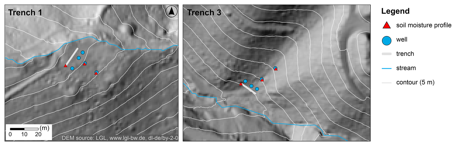
Figure 1 Location of the trenches, wells, soil moisture profiles and streams.

The climate is temperate, without a dry season and characterized by warm summers according to the Köppen classification (Cfb) (Peel et al., 2007). The mean annual temperature and precipitation are 11 °C and 836 mm yr⁻¹, respectively (2003–2023; weather station of the German Meteorological Service (DWD) in Freiburg located ca. 7 km north from the study area). The summer months May to August are characterized by the highest mean monthly rainfall as well as the highest mean rainfall intensity (convective storms) (2003–2023; DWD Freiburg).

The bedrock is formed by Migmatite and Paragneiss at T1 and by Migmatite at T3 (LGRB-Kartenviewer, 2024). In both locations the bedrock is overlain by unconsolidated periglacial slope deposits in which Cambisols have developed.

T1 was excavated into the slope deposits and does not reach the bedrock. From the surface down to 0.6 m below ground level (m b.g.l.) (depth of deepest soil sample), the soil is characterized by a high concentration of angular granule to cobble-sized clasts (i.e. diameter 2–256 mm) supported by a loam matrix (see Table 1 for soil properties). From 0.6 m b.g.l. to the base of the trench at 2.7–2.9 m b.g.l. the visual inspection showed an overall homogeneous material. Of particular interest is the soil colour of the trench face, which is not homogeneous. Besides the expected darker brown upper layer, a vertical ca. 2–3 m wide zone located on the southwest (right) side of the trench is characterized by a distinct dark bluish-grey colour. This coloration, which continues northeast (left) along the bottom portion of the trench, is a clear indication of waterlogged soils (Smirnova and Kozlov, 2023). The colour is typical of iron compounds that form in saturated soils under anaerobic (reducing) conditions (Schmidt and Ahn, 2019). The presence of such a long-lasting saturated zone matches well with our trenchflow and water level observations as well as the presence of a small intermittent spring located a few meters upslope of the trench.

Table 1 Soil Properties at trench 1 and 3.

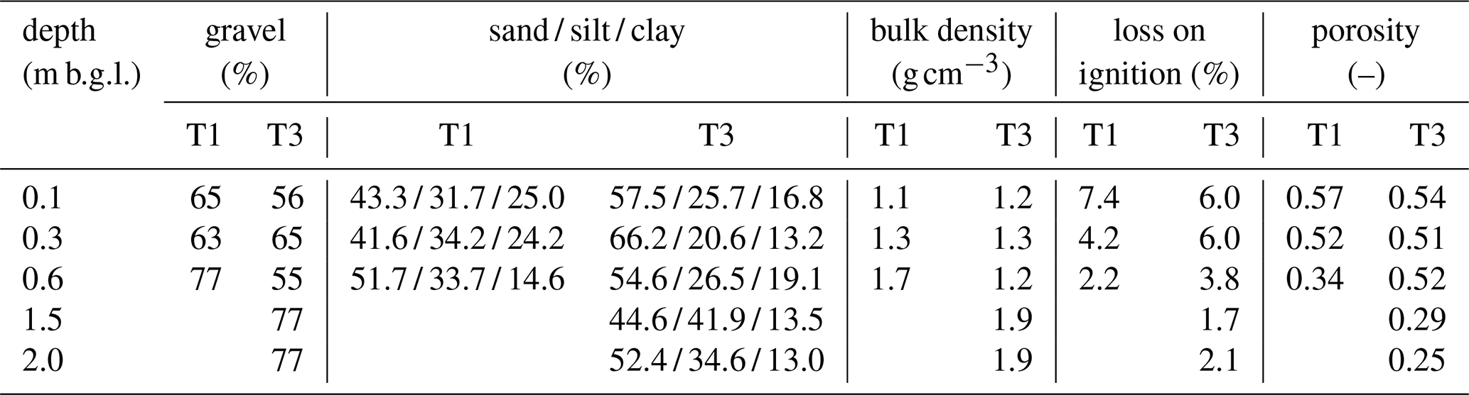
The reported depths represent the midpoint of the 5 cm sampling interval. Analysis method: gravel = dry sieve, sand = wet sieve, silt and clay = laser diffraction, porosity = from fitted water retention curve obtained from HYPROP 2 and WP4C (METER-Group) measurements. Grain size classification: gravel >2 mm, sand 2000–63 µm, silt 63–5.9 µm, clay <5.9 µm. The silt-clay cut-off of 5.9 µm was used instead of 2 µm to align laser diffraction results with those obtained from traditional sedimentation analyses (Faé et al., 2019).

At T3 the top 0.4 to 0.6 m of the soil is very poorly sorted and mainly composed of large (up to cobble-sized) angular clasts with a sandy loam matrix (see Table 1). Below this zone the amount and size of larger clasts gradually decreases (inverse grading) and the soil becomes more homogeneous and richer in silt (loam). This textural change is also supported by the water-retention analysis and soil density measurements of soil sampled at the trench face. The base of the unconsolidated slope deposits is defined by the weathered bedrock. At the trench, the interface between slope deposits and bedrock dips towards northwest (left trench side) while the elevation of the ground surface remains somewhat constant. This translates to an increase in thickness of the slope deposits from a few decimetres on the right side of the trench to more than 2 m on the left side of it. The thickness of the coarser upper layer remains fairly constant throughout the trench. Drilling samples of boreholes located ca. 12 and 21 m upslope of the trench also showed the presence of this coarse upper layer (thickness ca. 0.25–0.6 m) overlying a finer, more homogeneous sediment. This suggests that the hillslope directly above the trench is covered by a mostly continuous coarse-grained and thus highly permeable layer overlying a finer, less permeable one. The bedrock' s permeability is classified as very low according to thematic geological maps (LGRB-Kartenviewer, 2024) and thus likely acts as an aquitard/aquiclude in this hydrogeological setting.

The two hillslopes are covered by a mixed forest. The canopy above T1 is dominated by hornbeam (Carpinus) and spruce (Picea), interspersed with a few ash (Fraxinus) and beech (Fagus) trees. With higher elevation the proportion of coniferous trees increases giving rise to a coniferous-dominated forest. Young spruce trees make up most of the understory which is moderate above the trench and thins out further upslope. Strong winds toppled a few trees (mostly hornbeam) on the outer northern part of the hillslope during the observation period.

At T3 a mix of predominantly hornbeam (Carpinus) and fir (Abies) is found with a few robinia (Robinia) and ash (Fraxinus) on the lower part of the hillslope. The understory is thin and made up mainly of young fir trees. On both hillslopes the forest floor is covered by litter of deciduous and needle leaves as well as by some deadwood.

2.2 Experimental design

Two slope-perpendicular trenches, measuring 11 and 14 m in length and up to 2–3 m in depth, were installed to quantify SSF (Table 2). Photographs of the trenches during construction are provided in Appendix A. As illustrated in Fig. 2 and documented in Appendix A, SSF was collected from two different depth horizons using drainage mats positioned along the trench face. At the bottom of the drainage mat a pond liner was inserted 5–10 cm into the trench face with an upward angle. The pond liner was then folded around a drainage pipe, forcing the collected water into the pipe (see cross section in Fig. 2). The pipes were slightly tilted to route the water to the measuring equipment. Once the drainage system was installed, the trench was backfilled. The geometry of the two trenches (see Table 2) differs due to the different site characteristics.

Table 2 Trench properties.

Figure 2 Experimental design of the trenches. Blue arrows show water flow directions.

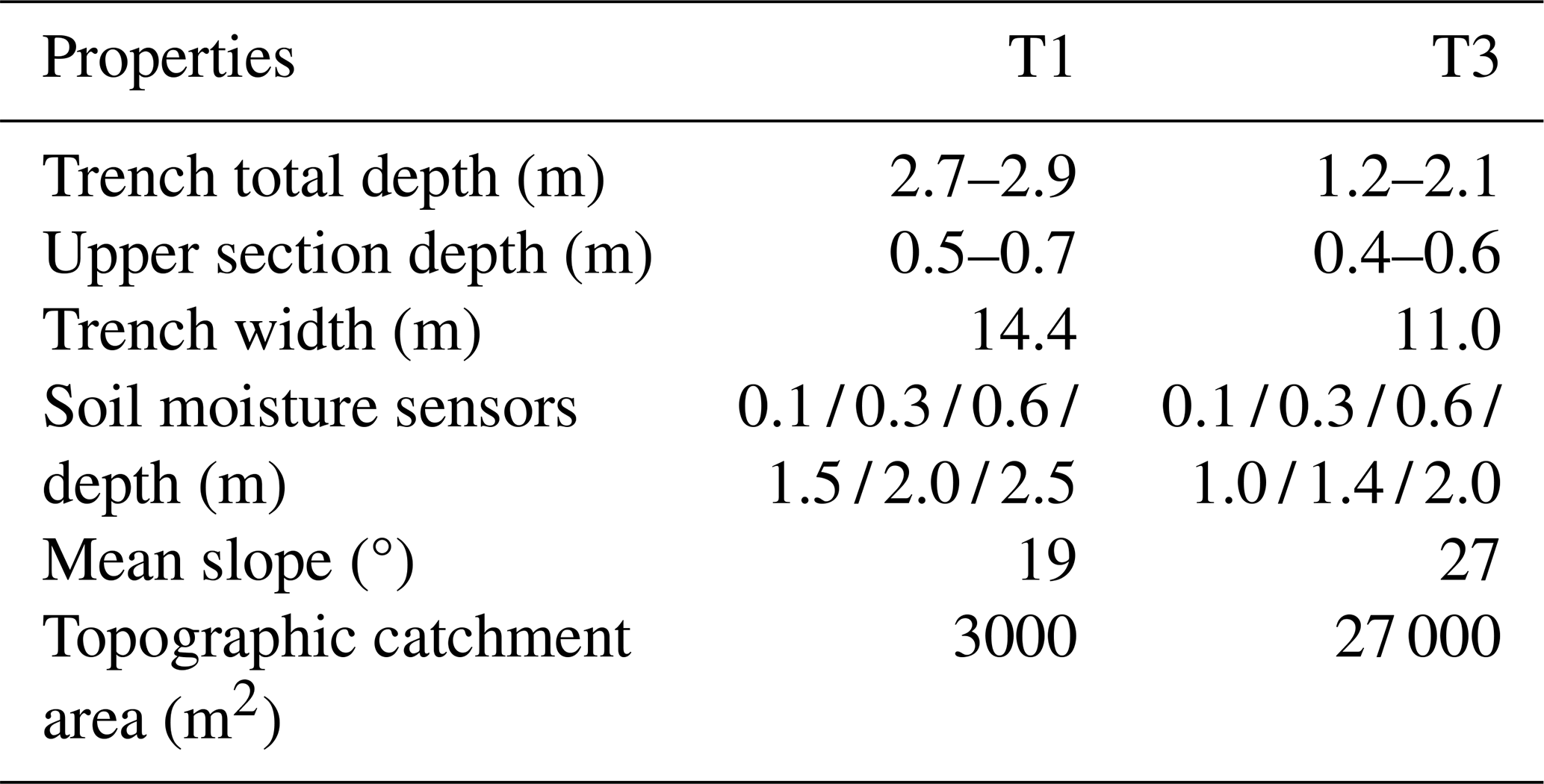
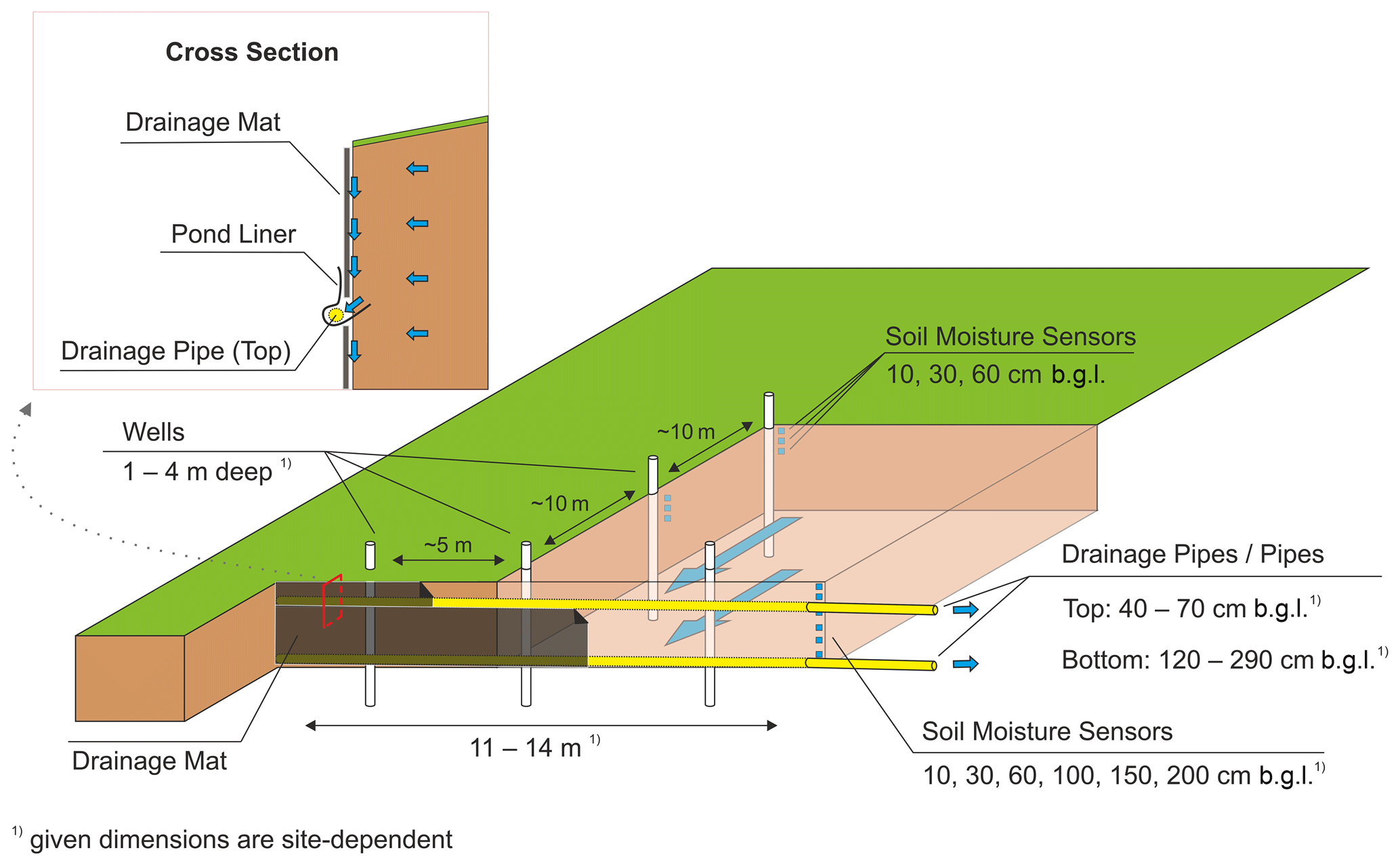
The trench discharge was gauged using a set of two custom-built tipping buckets. Each tipping bucket is able to measure flowrates of up to ca. 450–500 L h⁻¹. Based on gravimetric reference measurements (bucket weighing and timed collection), the combined standard (1σ) uncertainty for discharges <300 L h⁻¹ is ca. ±4 L h⁻¹. For higher discharges, uncertainty was not quantified but is expected to increase and discharge may be underestimated due to systematic errors (e.g. continuous inflow into the cavity of the tipping bucket while it is tipping; see Schwamback et al., 2022). Since discharges greater than 450 L h⁻¹ were sporadically observed at the bottom section of T3, a custom-made V-Weir, built following the design proposed by Stewart et al. (2015), along with a vented pressure transducer (Truebner GmbH), was installed towards the end of the study period from 27 May to 25 June 2024. Along with the flow rate, the temperature and electrical conductivity of the trenchflow was also continuously measured. Above the trench, the shallow groundwater level was monitored using five observation wells; three wells were aligned 2–5 m above the trench and an additional two were located ca. 10 and 20 m further upslope. The 6 cm-wide well boreholes were drilled using a hand-held percussion hammer. The depths of the boreholes vary between 1 to 4 m, as difficult drilling conditions (e.g. large boulders) sometimes limited the drilling depth (tool refusal depth). All boreholes were equipped with 5 cm diameter, fully slotted PVC pipes wrapped in geotextile. Where possible, the annular space between pipe and borehole wall was filled with quartz sand (≤2 mm). Each well was equipped with a capacitance water level sensor or a pressure transducer (Truebner GmbH) to monitor the water level. The water content and temperature of the soil was measured in three vertical profiles with TDT sensors (SMT100, Truebner GmbH). The deepest profile (2–2.5 m) was installed along the edge of the trench-face a few decimetres away from the drainage mat (Table 2). The two shallower profiles were set up near the two upper wells and had sensors installed at 10, 30 and 60 cm b.g.l. All trench data (trenchflow rate, electrical conductivity, temperature, water level and water content) were continuously measured, predominantly using a 10 min logging interval.

Meteorological data was collected from a weather station set up in an open field near T1 and ca. 500 m from T3 at an elevation of ca. 350 m a.s.l. ($\mathrm{47}\mathit{°}{\mathrm{57}}^{\prime }{\mathrm{25}}^{\prime \prime }$ N; $\mathrm{7}\mathit{°}{\mathrm{50}}^{\prime }{\mathrm{17}}^{\prime \prime }$ E). Rainfall was measured with a tipping bucket rain gauge (Thies) using a 5 min interval. Two gaps in the timeseries (12 % of the total rainfall data) were filled with data from a station located ca. 2 km N-NW, equipped with a tipping bucket rain gauge (Young 52203). An event-based comparison between the two stations showed good agreement in the precipitation data, despite the secondary station being operated with a 10 min logging interval.

2.3 Data analysis

2.3.1 Data pre-processing

The analysed data was collected over a period of ca. 2 years from 25 August 2022 to 1 October 2024. The trenchflow data used for the analysis required some pre-processing. Short data gaps in the timeseries of T1 and T3 (e.g. due to sensor maintenance) were filled using linear interpolation. Besides a few exceptions, most gaps were shorter than 2 h. Outliers, caused by sporadic malfunctions of the tipping-bucket logging system, were manually filtered out and the gaps filled using the same linear approach. Longer gaps (e.g. due to sensor failure) were not filled and excluded from the analysis. Nearly all the data was recorded using a 10 min interval with some exceptions of 15 and 20 min. Therefore, to homogenize the timeseries the time was resampled into 10 min intervals using a linear interpolation approach. Since this study focuses on liquid precipitation, periods characterized by snowfall and snowmelt were excluded from the analysis (10 December 2022–19 February 2023 and 5–22 January 2024). These periods were identified based on data from a nearby snow-measuring DWD weather station (Freiburg) as well as field observations and trenchflow data. Only periods with data available for both trench sections (top and bottom) were considered. During a handful of SSF events trenchflow exceeded the capacity of the tipping buckets of ca. 450–500 L h⁻¹ leading to erroneous plateaus in trenchflow rate. These events were not included in the analysis. Nonetheless, a few exceptions were made for events that were not obviously cut off despite the observed extremely high flow rates. The rainfall timeseries, derived from the two weather stations (see previous section), was resampled using a 5 min interval. Soil moisture dynamics were monitored using SMT100 sensors (Truebner GmbH), which measure temperature and dielectric permittivity. The volumetric water content (VWC) was derived using the Complex Refraction Index Model (CRIM) to account for the influence of temperature on permittivity (see Appendix B for details). Short data gaps in the resulting VWC timeseries (e.g. due to sensor maintenance) were filled using a linear interpolation approach, while longer gaps were not filled. Most gaps were shorter than 2 h.

2.3.2 Rainfall event delineation

To carry out the event-based analysis, rainfall events had to be delineated from the continuous rainfall timeseries. For this purpose, the commonly used minimum inter-event time (MIT) method in conjunction with the minimum rainfall depth (MRD) criteria was applied (Dunkerley, 2008). According to the MIT method, each rainfall event has to be preceded and succeeded by a fixed minimum dry period (MIT) (Brasil et al., 2022). In other words, two rainfall occurrences are considered part of the same event if they are separated by a time period shorter than the MIT. In the literature MIT values range from 3 min to 24 h depending on the site and application, and although values between 6 and 8 h are the most commonly adopted it is evident that no recommended MIT value exists (Dunkerley, 2008). Despite this, the MIT value heavily influences the number of delineated rainfall events as well as their characteristics (e.g. duration, depth, intensity) (Brasil et al., 2022). Therefore, different MITs were applied to our dataset and the results were evaluated. In our case, an MIT of 6 h yielded the most satisfactory results, as each SSF initiation was mostly associated with a single well-defined rainfall event and a relatively low number of single-tip events (i.e. rainfall events consisting of only one bucket tip) was generated. In comparison, longer MITs generated larger rainfall events spanning multiple SSF initiations while shorter MITs led to a greater segmentation of sometimes clearly associated rainfall pulses. Once the rainfall events were delineated (MIT of 6 h), the MRD criteria was applied to eliminate single-tip events, resulting in an MRD of 0.105 mm in our case.

2.3.3 Subsurface stormflow event delineation

Several methods from manual to fully automatic have been developed to delineate storm events from continuous streamflow records (Millar et al., 2022). However, most automatic and semi-automatic methods were developed for larger rivers, not for small, flashy, intermittent headwater creeks, whose complex flow dynamics more closely resemble those observed at the trenches (trenchflow). As a result, these methods often require somewhat smoother hydrographs, the presence of a continuous baseflow and in some cases well-defined recession limbs (Blume et al., 2007; Koskelo et al., 2012; Mei and Anagnostou, 2015). Additionally, only a handful of these methods integrate precipitation data linking rainfall events to stormflow events (Koskelo et al., 2012; Mei and Anagnostou, 2015). Automated methods for delineating SSF events based on trenchflow signal (e.g. not using a nearby stream to define the start and end of stormflow events) were not found in literature; authors dealing with trenchflow hydrographs generally use manual delineation methods or at least do not mention the use of automated methods (e.g. Fu et al., 2013; Han et al., 2020; Tani, 1997).

In this study, due to the long time series and to ensure the most objective delineation possible, a semi-automatic separation method was developed. The new method was tailored to the observed trenchflow, which was flashy, quite noisy and characterized by periods with and without “baseflow”. Furthermore, the method allowed to link rainfall events to SSF events and further classify them. It scans the trenchflow discharge time series from the start of each rainfall event, and if the onset of an SSF event is detected, it links the two. If baseflow is absent, the onset of flow marks the event start. If baseflow is present, the start is detected by assessing the increase in discharge over two time windows (short and long) relative to a threshold. The end of SSF events is detected by analysing the change in discharge and its standard deviation over a fixed time window as well as considering the flowrate preceding the events. The delineation method is described more in detail in Appendix C.

The automatic delineation results were satisfactory. For T1 and T3 on average only ca. 4 % of the starts had to be added, 15 % had to be removed and 12 % had to be re-positioned, while 21 % of the ends had to be re-positioned.

2.3.4 Classification of subsurface stormflow and rainfall events

After the detection of starting and ending points in the trenchflow time series, the SSF events were classified into simple events and subevents (Fig. 3). Simple SSF events are “stand alone” events that do not overlap with the preceding or subsequent events and are triggered by one rainfall event. Subevents are also associated with a triggering rainfall event but, unlike simple events, overlap with SSF events detected before and/or after (i.e. they might start before the end of the preceding SSF event and/or end after the start of the subsequent SSF event) and thus are part of a larger, more complex SSF event. For this reason, two or more overlapping SSF events (i.e. subevents) are grouped into so-called complex SSF events.

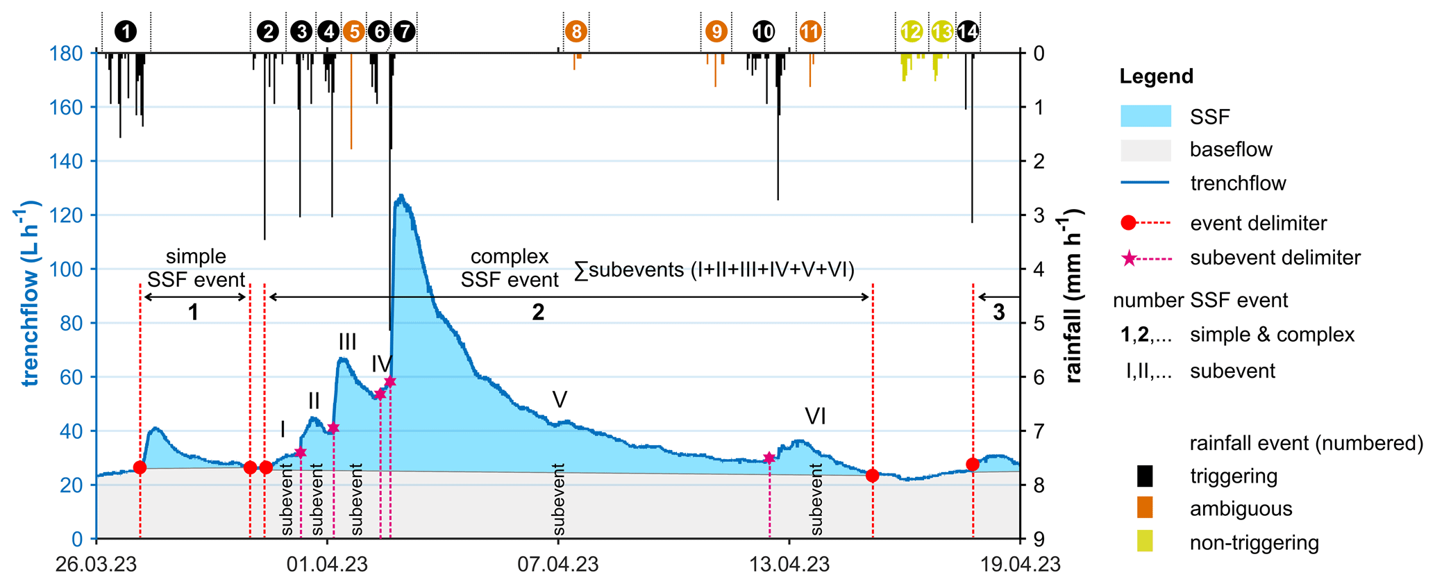
Figure 3 Classification of SSF and rainfall events. Simple SSF events are “stand alone” events, while subevents are interlinked with each other forming complex SSF events. Each triggering rainfall event is associated with a specific subevent or simple SSF event. Ambiguous rainfall events fall within a simple or complex SSF event, but do not trigger a subevent. Non-triggering rainfall events fall outside of the delineated simple or complex SSF events and are not associated with any SSF event.

Rainfall events are classified into three categories: triggering, ambiguous and non-triggering (Fig. 3). Triggering events are all rainfall events that trigger SSF events (simple events and subevents), and are therefore linked to the start of SSF events. For example, in Fig. 3 the simple SSF event no. 1 is associated with the triggering rainfall event no. 1, and the subevent no. III is associated with the triggering rainfall event no. 4. Non-triggering rainfall events are events that neither induce nor contribute to SSF events and therefore occur outside of delineated SSF events (e.g. rainfall events nos. 12 and 13 in Fig. 3). Ambiguous events are events that occur within SSF events but for which no SSF starting point could be detected, as they do not lead to a noticeable increase in trenchflow (e.g. rainfall event nos. 5, 8, 9 and 11 in Fig. 3). Nevertheless, they may still contribute to trenchflow during the SSF event. Hence, they are considered together with the triggering events for the calculation of the total rainfall amount associated with simple or complex SSF events (e.g. rainfall event nos. 2–11 are considered for the complex SSF event no. 2 in Fig. 3). However, only the triggering rainfall events are used to compute the rainfall intensity associated with simple or complex SSF events (e.g. rainfall event nos. 2, 3, 4, 6, 7, 10 are considered for the calculation of the intensity associated with the complex SSF event no. 2). Further details on how rainfall and SSF metrics were obtained and linked in the analysis are presented in the next section (Sect. 2.3.5).

2.3.5 Rainfall and SSF event characteristics

For each rainfall event (triggering, ambiguous, non-triggering) the total depth (P_tot) was calculated. The mean intensity (I_m), I₅, I₃₀ and I₆₀ (i.e. max. 5-, 30- and 60-min rates) were calculated only for triggering rainfall events. For rainfall events that occurred during the period covered by the secondary weather station, I₅ was not considered due to the 10 min logging interval of this station. Furthermore, we calculated the cumulative depth (P_tot) of all rainfall events (triggering and, where present, ambiguous) associated with the respective simple or complex SSF event. This cumulative depth was used when analysing the relationship with SSF metrics describing simple and complex SSF events: mean trenchflow rate ($\stackrel{\mathrm{‾}}{Q}$), total SSF volume (V_tot) and minimum contributing area (MCA). Moreover, rainfall intensities (I_m, I₅, I₃₀ and I₆₀) of triggering events associated with the same complex SSF event were additionally averaged (e.g. for two triggering events A and B associated with the same complex SSF event, the I₃₀ intensity was calculated as the arithmetic mean of the triggering events: ($I_{\mathrm{30}\mathrm{A}}+I_{\mathrm{30}\mathrm{B}})/\mathrm{2}$). This averaging was performed to examine how rainfall intensity influences properties related to the entire complex event ($\stackrel{\mathrm{‾}}{Q}$, V_tot, MCA). Figure 4b gives an overview of the SSF metrics and the type of SSF events for which they were computed as well as the type of rainfall events considered to derive the associated P_tot and intensities. The total SSF volume was computed for simple and complex SSF events after subtracting the baseflow, which was separated from the event runoff using the straight line method (Fig. 4a) (Maidment, 1993). Following this method, the timestep preceding the start of the event and the endpoint were connected through a straight line. The minimum contributing area (MCA), also called stormflow ratio, was calculated, as following (Dickinson and Whiteley, 1970):

$$\begin{array}{}\text{(1)}& \text{MCA}=V_{\text{tot}}/P_{\text{tot}}\end{array}$$

The MCA represents the minimum area required to produce the observed SSF volume under the assumption that 100 % of rainfall on that area is converted to SSF. For example, 10 mm rainfall producing 20 L of SSF corresponds to an MCA of 2 m². The contributing area is defined here as the area that contributes to the SSF collected at the trench during the SSF event. This area is expected to be larger than the MCA because only a fraction of rainfall over the contributing area typically contributes to the generation of SSF, due to losses to interception, soil moisture storage, vertical leakage, etc. The subsurface runoff coefficient (C_sub) is directly related to MCA ($C_{\text{sub}}=\text{MCA}/\text{SSF}$ catchment area); however, because the extent of the SSF catchment area is not known, it can only be estimated by dividing MCA by the topographically derived catchment area.

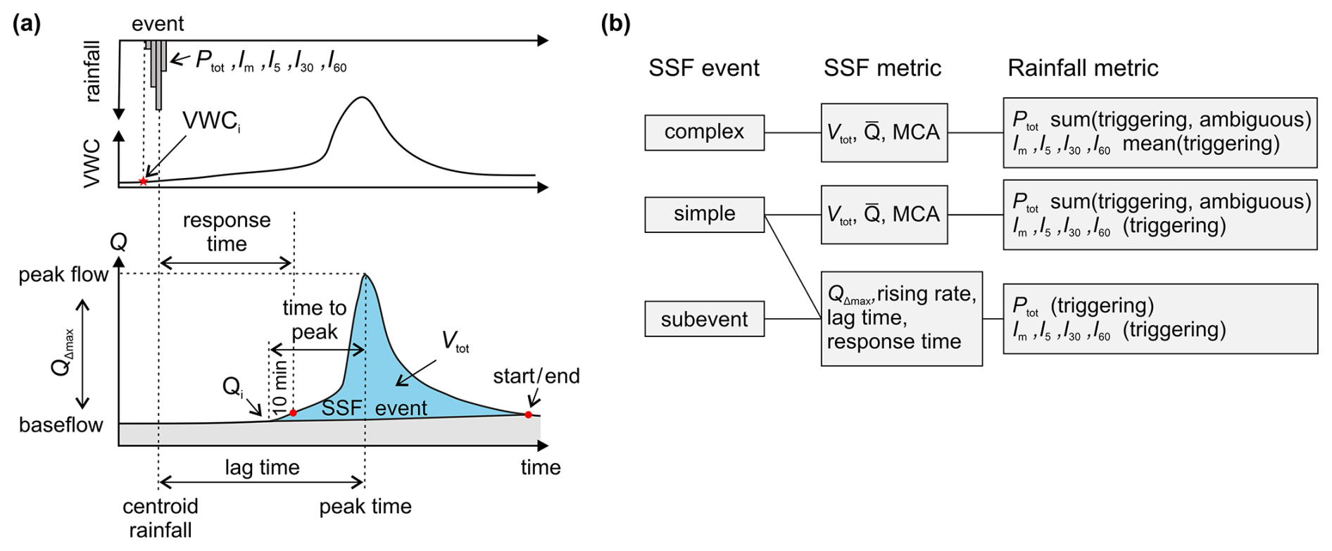
Figure 4 (a) Definition sketch of the SSF, rainfall and antecedent conditions metrics used in the event-based analysis. (b) Overview of the SSF metrics, the type of SSF events for which they were computed, and the type of rainfall events considered for the calculation of the associated P_tot and intensities. When analysing V_tot, $\stackrel{\mathrm{‾}}{Q}$ and MCA the considered P_tot is obtained by summing the rainfall of the triggering and ambiguous events associated with the respective simple or complex SSF event, whereas only the triggering events are considered for the calculation of the intensities (for complex SSF events, the intensities are averaged across the associated triggering events). For the remaining SSF metrics, the P_tot and intensity of the triggering event associated with the subevent/simple SSF event are considered in the analysis.

The remaining SSF metrics (Q_Δmax, rising rate, response time and lag time) were calculated for simple events and subevents, and analysed against the rainfall characteristics (P_tot, I_m, I₅, I₃₀ and I₆₀) of the triggering rainfall event associated with the respective simple or sub-SSF event (see Figs. 3 and 4). The maximum increase in trenchflow rate (Q_Δmax) is the difference between the max. observed trenchflow rate and the initial trenchflow rate (Q_i) (i.e. flow preceding the event; see also Sect. 2.3.6 Antecedent conditions). The time to peak is defined as the period between the timestep preceding the start of the event and the max. trenchflow rate (peak flow). It is used to calculate the rising rate, which is obtained by dividing Q_Δmax by the time to peak. Very small events having $Q_{\mathrm{\Delta }max}<\mathrm{3}$ L h⁻¹ were not considered for the rising rate calculations. The response time refers to the interval between the centroid of the rainfall event and the start of the SSF event, whereas the lag time is the time between the centroid and the maximum observed trenchflow rate (peak flow).

In five cases, the rising phase of a subevent was interrupted by a successive subevent, preventing the potential peakflow of the preceding subevent from being reached. As a result, for these subevents the peak-dependent metrics were not considered. Moreover, occasionally simple events and subevents were characterized by a well-defined double peak with a higher second peak. In these and other exceptional cases (10 events) the Q_Δmax was used in the analysis but the time-dependent metrics (e.g. rising rate) were not, as the double peak nature of the event would lead to inconsistent results.

2.3.6 Antecedent conditions

The antecedent wetness of the subsurface preceding the SSF events was characterized using soil moisture and trenchflow data. More specifically, the initial average volumetric water content (VWC_i), antecedent soil moisture index (ASI) and initial trenchflow rate were considered.

The VWC_i was calculated using a weighted average approach as described in Pangle et al. (2014):

$$\begin{array}{}\text{(2)}& {\text{VWC}}_{\mathrm{i}}={\displaystyle \frac{{\sum }_{j=\mathrm{1}}^{\mathrm{6}}{\mathit{\theta }}_j{H}_j}{H_{\text{tot}}}}\end{array}$$

where θ₁ to θ₆ represent the volumetric water content measured at different depths (see Table 2), H₁ to H₆ are the soil layer thicknesses that each sensor is assumed to represent, and H_tot is the total considered depth. For each sensor, H is calculated by dividing the distance between the sensor above and below by two. For the uppermost and lowermost sensors, the distance from the adjacent sensor was used. For example, for sensors depths of 10, 30, 60, 150, 200 and 250 cm the associated H would be 20, 25, 60, 70, 50 and 50 cm, respectively, and the total depth 275 cm. Since the soil moisture at 10, 30 and 60 cm b.g.l. was measured at three different locations (i.e. at three soil moisture profiles: S1, S2 and S3), a mean value for each depth was computed and used in the depth-averaging procedure described above. Periods with missing or unreliable data were handled differently depending on the depth of the affected sensor. If sensors installed at depth 4, 5 or 6 had a data gap the VWC_i was not computed for that time period. On the other hand, for the shallower depths 1, 2 and 3 (i.e. 10, 30 and 60 cm b.g.l.) if data from one or two sensors was missing, data from the remaining working sensor/s was used. The total equivalent water storage of the soil profile in mm can be obtained by multiplying VWC_i by H_tot.

The Antecedent Soil-moisture Index (ASI) was calculated using the following equation (Haga et al., 2005; Penna et al., 2015):

$$\begin{array}{}\text{(3)}& \text{ASI}=({\mathit{\theta }}_{\mathrm{1}}\cdot \mathrm{200})+({\mathit{\theta }}_{\mathrm{2}}\cdot \mathrm{250})+({\mathit{\theta }}_{\mathrm{3}}\cdot \mathrm{300})\end{array}$$

where θ₁, θ₂ and θ₃ represent the volumetric water content measured by the sensors at depths of 10, 30 and 60 cm b.g.l., respectively; they are multiplied by the layer thickness (in mm) that the sensors are assumed to represent (analogous to H in Eq. 2). As for Eq. (2), since soil moisture at 10, 30 and 60 cm b.g.l. was measured at three different locations, the mean value for each depth was used in the calculations. Data gaps were handled as described for Eq. (2). The ASI, which represents the soil water storage (mm) in the upper soil layer, can be added to the total precipitation depth (P_tot+ASI), allowing us to describe the total rainfall and initial soil moisture conditions using one value. However, ASI is strongly dependent on the thickness of the considered soil profile (750 mm in our study); under identical moisture conditions, a deeper profile yields a larger ASI. Hence, the absolute value and event-to-event variability of ASI can be on the order of hundreds of mm, whereas P_tot is typically on the order of tens of mm. Consequently, ASI can be large relative to P_tot, so that antecedent conditions may receive disproportionate weight in the composite variable P_tot+ASI when correlations with SSF metrics are analysed. We therefore introduced a second composite variable where ASI is weighted: P_tot+ASI_adj (see Sect. 2.3.7). Both the VWC_i and ASI were computed for the timestep preceding the triggering rainfall event. For complex SSF events the VWC_i and ASI associated with the first triggering rainfall event were used to represent the antecedent wetness conditions of the complex event. The trenchflow before the start of SSF events was also considered. The initial trenchflow rate (Q_i) was computed by averaging the flow over a period of 30 min preceding the start of sub- and simple SSF events. For complex SSF events the initial trenchflow rate of the first subevent was considered.

2.3.7 Correlation analysis

The Spearman rank correlation coefficient (r_s) was used to quantify the degree of correlation between the metrics describing rainfall event characteristics, antecedent conditions, and SSF event characteristics. Correlation coefficients were not calculated for metric pairs that were not mathematically independent by construction and were therefore prone to spurious self-correlation. Pairwise correlations of V_tot, $\stackrel{\mathrm{‾}}{Q}$ and MCA with Q_Δmax, rising rate, lag time and response time were calculated only for simple SSF events, because this full set of metrics is available only for this type of SSF event (Fig. 4b). The correlation with the composite variable (P_tot+ASI) was also computed. However, since the results suggested that ASI was overrepresented in the composite variable (e.g. at T1 V_tot showed a smaller correlation with P_tot+ASI than with P_tot alone), ASI was adjusted (ASI_adj) using a metric-specific weighting factor (w), which was optimized to maximize the Spearman correlation of the composite variable ($P_{\text{tot}}+w\cdot \text{ASI}$) with the other SSF metrics. This approach allowed us to assess the relative importance of antecedent wetness conditions within the composite variable when analysing its correlation with SSF metrics. The Spearman rank correlation was chosen to capture any monotonic relationship, as the observed relationships were sometimes nonlinear (e.g. exponential) and thus would have not been identified by the more restrictive Pearson correlation analysis. Given the large number of tested correlations, to keep the overall α-level at 0.05, following Bonferroni's correction the per-test significance level was obtained by dividing 0.05 by the total number of tested correlations (97 for each trench) (Curtin and Schulz, 1998). Correlations were considered statistically significant when the p-value was smaller than 0.0005.

Uncertainty in Spearman rank correlations was quantified using a bootstrap approach (Haukoos and Lewis, 2005). For each pair of metrics, the dataset was resampled with replacement (i.e. data points were randomly selected from the original dataset and could be selected multiple times) to generate 1000 bootstrap datasets (recommended ≥250 datasets; Efron and Tibshirani, 1986). Spearman's r_s was then computed for each resample, and a 95 % confidence interval (CI) was obtained using the percentile method as the 2.5 and 97.5 percentiles of the bootstrap distribution of r_s. The confidence intervals of the Spearman rank correlations are presented in Appendix D.

To evaluate whether the correlation between Y and two alternative metrics (X₁ and X₂) improved, we computed the difference between the corresponding Spearman rank correlations, $\mathrm{\Delta }{r}_{\mathrm{s}}=r_{\text{s2}}-r_{\text{s1}}$, where $r_{\text{s1}}=r_{\mathrm{s}}(Y,X_{\mathrm{1}})$ and $r_{\text{s2}}=r_{\mathrm{s}}(Y,X_{\mathrm{2}})$. Uncertainty in Δr_s was quantified using a bootstrap approach (Wilcox, 2016). The dataset (Y, X₁, X₂) was resampled with replacement to generate 1000 bootstrap datasets; for each resample, Δr_s was computed and stored. A 95 % confidence interval for Δr_s was then obtained using the percentile method. An improvement was considered supported when the 95 % confidence interval for Δr_s (CI_Δrs) lay entirely above zero. This analysis was performed only for selected metric pairs.

Since $\text{MCA}=V_{\text{tot}}/P_{\text{tot}}$, a direct regression of MCA against P_tot is susceptible to spurious self-correlation because a ratio is correlated with its own denominator (Kenney, 1982). To avoid ratio–denominator regression, we fit V_tot directly as:

$$\begin{array}{}\text{(4)}& V_{\text{tot}}=a\cdot P_{\text{tot}}^{\mathrm{2}}+b\cdot P_{\text{tot}}\end{array}$$

This formulation implies a precipitation-dependent $\text{MCA}\left(P_{\text{tot}}\right)=a\cdot P_{\text{tot}}+b$, which we use for interpretation. Thus, a>0 indicates that MCA increases with P_tot, and the value of a quantifies the rate of this increase. The lower bound for P_tot in Eq. (4) follows from V_tot=0, which occurs at P_tot=0 and at $P_{\text{tot}}=-b/a$. The upper bound for P_tot derives from the limiting case where the equivalent depth $V_{\text{tot}}/\text{CA}$ (mm; with V_tot in litre and CA the catchment area in m²) equals P_tot, which occurs at $P_{\text{tot}}=(\text{CA}-b)/a$, provided that a>0 and CA>b. Equation (4) was fitted separately for SSF events (simple and complex) with dry and wet antecedent soil moisture conditions. To classify the events, the observed range of VWC_i was divided into four equal intervals. Events with VWC_i values within the upper quarter of this range were classified as wet, while those below the upper quarter were classified as dry. After fitting Eq. (4) for each trench separately, Eq. (4) was also fitted to the combined T1 and T3 dataset to test whether the difference in the quadratic coefficient (a) between trenches was statistically significant.

In general, uncertainty in the flow-rate measurements (see Sect. 2.2) is expected to increase scatter in the relationships, leading to lower correlation coefficients and wider confidence intervals, particularly for analyses involving the metrics V_tot and Q_Δmax. Moreover, systematic errors associated with tipping-bucket measurements likely led to an underestimation of the highest flow rates and, consequently, of the Q_Δmax and V_tot values of events associated with such high flows. The statistical analyses were carried out using MATLAB (The MathWorks Inc, 2021).

3 Results

3.1 Rainfall events characteristics

During the observation period a total of 236 and 262 rainfall events were analysed for T1 and T3, respectively. The difference in number arises from the asynchronous data gaps in the time series of the trenches, since rainfall events occurring during data gaps were not analysed. Each simple SSF event and subevent was associated with a specific triggering rainfall event (see Sect. 2.3.4). Figure 5a gives an overview of the precipitation rates of these individual triggering rainfall events. Some SSF metrics (e.g. V_tot) were not calculated for subevents but only defined for simple and complex events (Fig. 4b). Figure 5b shows the intensities of the triggering rainfall events associated with simple SSF events and the averaged intensities of the triggering rainfall events belonging to the same complex SSF event. Thus, one intensity value (e.g. I₅) was assigned to each SSF event, whether simple or complex. As expected, the rates decreased from I₅ to I_m and were quite similar for the two trenches.

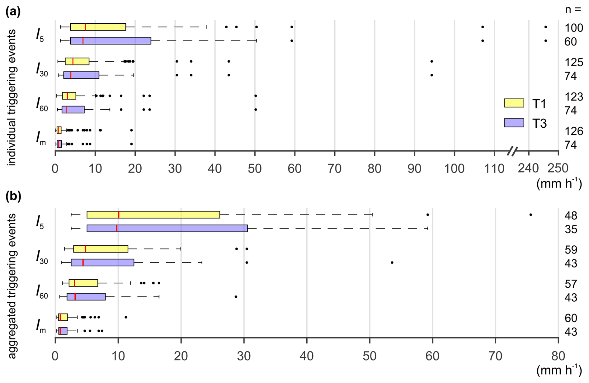
Figure 5 Overview of the rainfall rates of triggering rainfall events; (a) individual triggering events, (b) triggering events aggregated by their association with simple or complex SSF events (for each complex SSF event, a single representative rainfall intensity was computed as the mean of the intensities of its associated triggering rainfall events). The sample size (n) is shown on the right of each boxplot. I₅, I₃₀ and I₆₀ are the max. 5, 30 and 60 min rates, respectively, and I_m is the mean rate. Note that panel (a) has a gap in the axis and that the axis limits differ between panels (a) and (b).

The rainfall depths of triggering, ambiguous, and non-triggering events are shown in Fig. 6a, while Fig. 6b shows the total depth calculated by considering all rainfall events (triggering and, where present, ambiguous) associated with the same simple or complex SSF event. Most triggering events were larger than 5 mm; however, smaller events were also identified. T3 was characterized by larger triggering and non-triggering events, suggesting a higher precipitation threshold for the activation of SSF at the site. Moreover, at T3 the aggregated triggering and ambiguous events (Fig. 6b) were usually characterized by a higher total rainfall amount compared to T1.

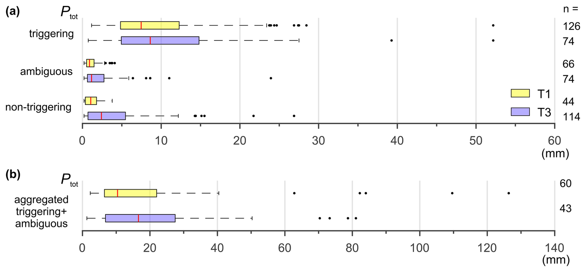
Figure 6 Overview of the (a) total rainfall depths of triggering, ambiguous and non-triggering rainfall events as well as of (b) total rainfall depth of the triggering and ambiguous rainfall events associated with each simple or complex SSF event (sum within each SSF event). The sample size (n) is shown on the right of each boxplot.

3.2 SSF events characteristics

In total, 38 simple events, 22 complex events and 88 subevents were identified at T1, whereas at T3, 29 simple events, 14 complex events and 45 subevents were identified. The characteristics of the analysed SSF events are presented in Fig. 7. Overall, the SSF response was similar at the two sites. However, at T3 the 75th percentile of V_tot, $\stackrel{\mathrm{‾}}{Q}$, MCA and Q_Δmax was higher, while it was longer for the response time and shorter for the lag time. Negative response times and lag times occur when the centroid of the rainfall event is located after the SSF start and peakflow time, respectively. The smaller response time at T1 indicates a faster SSF response and a smaller precipitation threshold, as the rainfall preceding the centroid was often sufficient to trigger SSF. The period between start of rainfall and start of SSF events (not plotted in Fig. 7) was sometimes as small as 5 min at both sites (5 min time resolution).

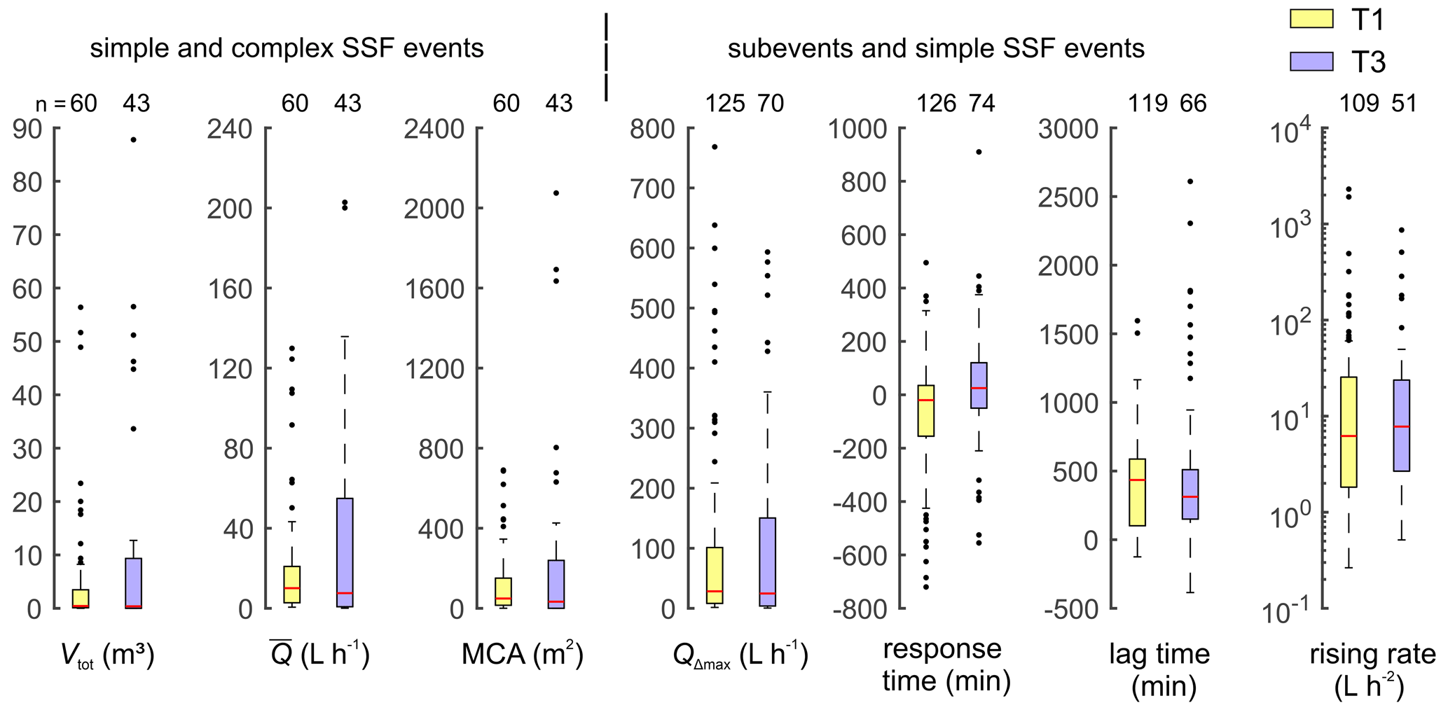
Figure 7 Overview of the characteristics of the analysed SSF events. The sample size (n) is shown above the boxplots. The difference in sample size of sub- and simple SSF event metrics for the same site results from the exclusion of some events from the calculation of specific metrics, according to the criteria outlined at the end of Sect. 2.3.5.

3.3 Correlation analysis

To study how different rainfall event characteristics and antecedent conditions influence the SSF response, the relationships between the descriptive metrics were analysed using the Spearman rank correlation (r_s). Figure 8 presents the resulting correlation matrix, with the correlations for T1 and T3 displayed in the upper right and lower left portions of the table (i.e. above and below the diagonal), respectively. The associated confidence intervals are shown in Fig. D1 of Appendix D.

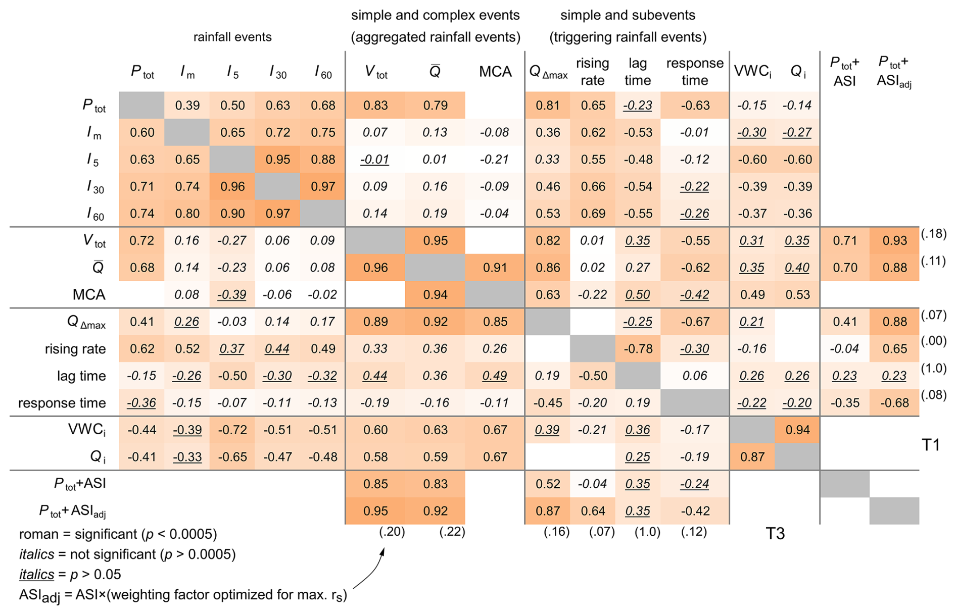
Figure 8 Spearman rank correlation coefficients between antecedent conditions, rainfall and SSF event characteristics at T1 (above diagonal) and T3 (below diagonal); the ASI adjustment factor is shown in parentheses. The associated confidence intervals are provided in Appendix D.

The correlation patterns of T1 and T3 show a high level of congruence, suggesting that the observed relationships are not site specific. The total precipitation showed a moderate relationship with the intensities, with relationship strength increasing from I_m to I₆₀. The correlation between VWC_i and Q_i was strong at both trenches. However, while at T1, due to the continuous baseflow, Q_i steadily increased with VWC_i starting from small VWC_i values, at T3 the increase started at higher VWC_i, since at this site baseflow was absent during dry conditions and thus lower VWC_i (data not shown). Comparing the correlation of the composite variable P_tot+ASI and P_tot with the other metrics showed that for P_tot+ASI the correlation was sometimes smaller than for P_tot (e.g. at T1, for Q_Δmax the r_s decreased from 0.81 to 0.41, with CI_Δrs<0), suggesting that the influence of the initial soil moisture conditions (i.e. ASI) was overemphasized in the composite variable. We therefore also tested the composite variable P_tot+ASI_adj, where ASI was weighted (adjusted) in order to achieve maximum correlation (see Sect. 2.3.7). The variables V_tot, $\stackrel{\mathrm{‾}}{Q}$ and Q_Δmax showed a marked improvement in correlation (supported by CI_Δrs>0) when the composite variable with the weighted ASI was considered, indicating a strong influence of the initial conditions on these variables. The improvement in correlation, the lower bound of CI_Δrs, and the weighting factor were higher at T3, suggesting that antecedent conditions play a stronger role at that site than at T1. For example, for Q_Δmax the correlation increased by 0.46 (CI_Δrs 0.22–0.70) at T3 but only by 0.07 (CI_Δrs 0.02–0.12) at T1, and the weights for ASI were roughly two times higher for T3 than for T1. For the variables rising rate and response time, the differences in correlation with P_tot and P_tot+ASI_adj were null or negligible, suggesting that initial conditions have little impact on these temporal metrics. Lag time was not correlated with P_tot, and the higher correlation obtained for the composite variable arise from its relatively higher correlation with VWC_i. The correlations with ASI are not shown in Fig. 8, since they were comparable to the ones with VWC_i.

3.3.1 Relationship between rainfall characteristics, total SSF volume and minimum contributing area (MCA)

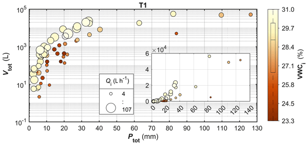
For both trenches, the V_tot, calculated for simple and complex SSF events, strongly correlated with P_tot, but the antecedent conditions also had a major influence on the SSF response. For similar P_tot the V_tot of events characterized by wet initial conditions (high VWC_i) were generally around one to three orders of magnitudes larger than their drier counterparts (lower VWC_i; see Figs. 9 and 10). Nevertheless, for SSF events associated with very large rainfall amounts (P_tot>50 mm) the influence of the antecedent conditions was often less pronounced and the P_tot–V_tot relationship was poor, as larger P_tot did not always imply higher V_tot. Visual inspection of the scatterplots revealed that initial trenchflow rate (Q_i) was valuable to explain some of the results of T3, where events characterized by similar VWC_i and P_tot generated different trenchflow amounts (e.g. events associated with P_tot 15–20 mm in Fig. 10). The rainfall amount to trigger a SSF response was minimal (2–3 mm) for both trenches. Nevertheless, the data suggests that the generation of somewhat larger events (V_tot>100 L) required ca. 5 mm of rainfall for wet antecedent conditions and ca. 10 mm for dry ones at T1, whereas at T3 the amount was ca. 5 and ca. 25 mm, respectively. The influence of the antecedent conditions was effectively accounted for using P_tot+ASI_adj, as shown in Figs. 11 and 12, where for both trenches wet and dry events tend to form one common trend.

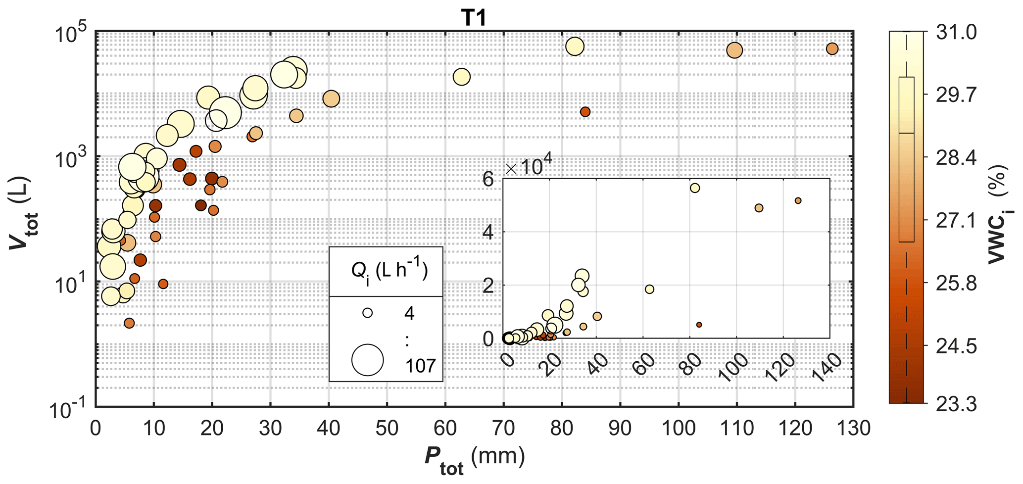
Figure 9 Total SSF volume (simple and complex SSF events) vs. total rainfall and antecedent conditions at T1. The insert shows the same data on a linear-linear scale. In the insert the marker size was reduced for better visualization. The antecedent conditions are represented by VWC_i (colour of markers) and Q_i (size of markers). The boxplot in the colorbar describes the distribution of VWC_i.

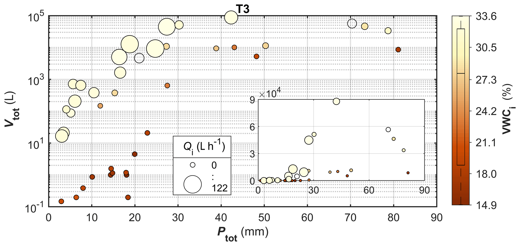
Figure 10 Total SSF volume (simple and complex SSF events) vs. total rainfall and antecedent conditions at T3 (event-based). The insert shows the same data on a linear-linear scale. In the insert the marker size was reduced for better visualization. The antecedent conditions are represented by VWC_i (colour of markers) and Q_i (size of markers). The boxplot in the colorbar describes the distribution of VWC_i.

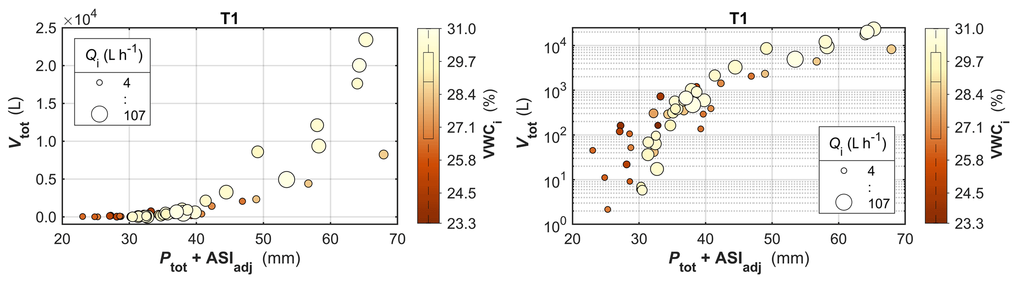
Figure 11 Relationship between total SSF volume (simple and complex SSF events) and total rainfall + ASI_adj at T1 (left plot is lin–lin and right plot is lin–log). The largest events are not included in the plots. The antecedent conditions are represented by VWC_i (colour of markers) and Q_i (size of markers). The boxplot in the colorbar describes the distribution of VWC_i.

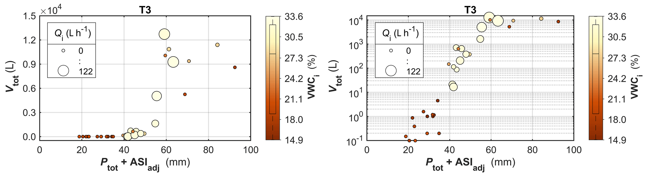
Figure 12 Relationship between total SSF volume (simple and complex SSF events) and total rainfall + ASI_adj at T3 (left plot is lin–lin and right plot is lin–log). The largest events are not included in the plots. The antecedent conditions are represented by VWC_i (colour of markers) and Q_i (size of markers). The boxplot in the colorbar describes the distribution of VWC_i.

Overall, at T1 the V_tot steadily increased with P_tot, whereas at T3, despite the general increase of V_tot with P_tot, this relationship appeared to undergo different stages, resulting in something like a step function on the semi-logarithmic plot (Figs. 9 and 10). More specifically, at T3, V_tot seems to increase markedly once P_tot exceeds ∼15 mm under wet antecedent conditions and ∼20 mm under dry antecedent conditions. This steeper increase appears to be preceded by a ∼10 mm window in which V_tot shows only a weak increase with P_tot (5–15 mm under wet conditions and 10–20 mm under dry conditions). However, we acknowledge that the number of events with wet antecedent conditions is limited in this range.

The initial conditions strongly influenced MCA, as under dry conditions MCA stayed relatively small, whereas under wet conditions MCA generally increased with P_tot reaching a maximum of ca. 700 and 2000 m² at T1 and T3, respectively (Fig. 13). The increase in MCA suggests an increase of the SSF contributing area. At T3 the MCA increased steeply for events associated with P_tot greater than ca. 15 mm and wet initial conditions. The maximum MCA corresponds to an estimated maximum C_sub (calculated using the topographically derived catchment area) of approximately 0.23 and 0.08 for T1 and T3, respectively.

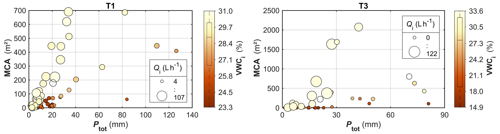
Figure 13 Relationship between MCA and total rainfall as well as antecedent conditions (simple and complex SSF events). The antecedent conditions are represented by VWC_i (colour of markers) and Q_i (size of markers). The boxplot in the colorbar describes the distribution of VWC_i.

To further explore the relationship between V_tot, P_tot, VWC_i, and indirectly MCA the simple and complex SSF events were separated into two groups (wet and dry) based on their associated VWC_i. Furthermore, for T1 and T3 only events associated with P_tot<50 mm were considered in the following analysis, as for those a more distinct V_tot vs. P_tot relationship was identified. In total, 92 % (T1) and 86 % (T3) of all simple and complex SSF events were included in the analysis. As shown in Fig. 14 and Table 3, within the considered range of P_tot, the linear fit between V_tot and P_tot was good at T1 (r² was 0.89 for wet events and 0.67 for dry events), and mediocre at T3 (r² was 0.46 and 0.56 for wet and dry events, respectively). Nevertheless, visually, the rate at which V_tot increases seemed to rise with P_tot, suggesting that a quadratic function would be better suited to represent the observed trend. This was evaluated by fitting the quadratic Eq. (4) to the data. Since Eq. (4) is the volume-based reformulation of a rainfall-dependent MCA (see Sect. 2.3.7), the good fit of Eq. (4) (Table 3) supports the interpretation that the contributing area increases with P_tot, which is consistent with the trend suggested by the MCA–P_tot plot (Fig. 13).

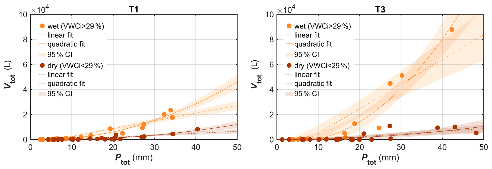
Figure 14 Total rainfall vs. total SSF volume of events (simple and complex) with dry and wet antecedent conditions, with the best linear fit (dashed line) and the fit of Eq. (4) (solid line).

Table 3 Coefficients with CI and r² of the fitted Eq. (4) and r² of the linear fit.

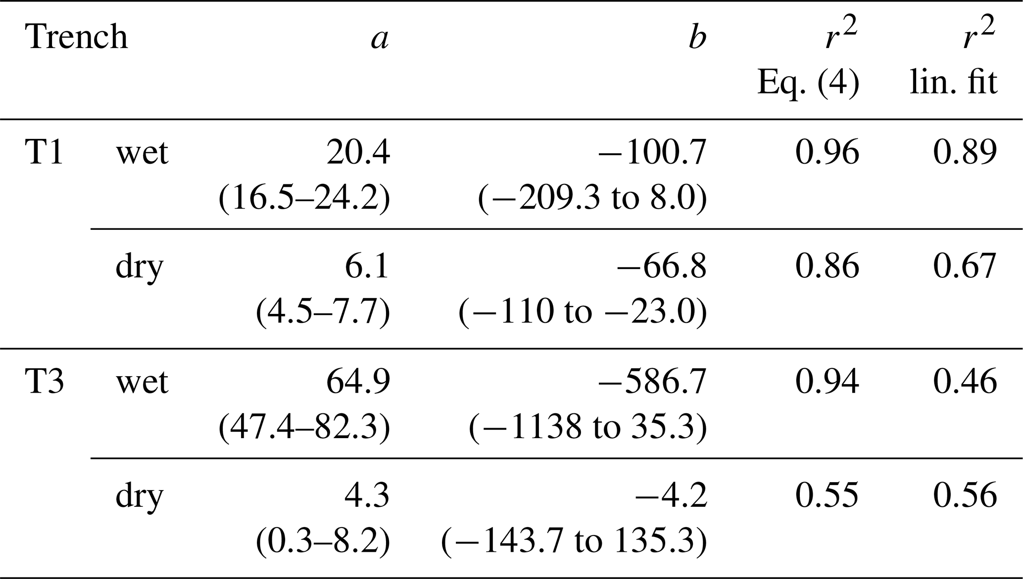
The very different quadratic coefficients (a) for wet and dry conditions suggest that initial soil moisture conditions strongly influence the rate at which the contributing area increases with P_tot.

The quadratic coefficient (a), computed for wet events, was significantly higher for T3 than for T1 (p<0.001), suggesting that under wet antecedent conditions the contributing area increases faster with P_tot at T3. Under dry antecedent conditions, however, the difference in a between T1 and T3 was not significant. Results from the quadratic V_tot–P_tot relationship (Eq. 4) are considered to be valid only up to P_tot∼50 mm (the upper limit of the fitted range).

Rainfall intensities (I₅, I₃₀, I₆₀ and I_m) showed a very poor and often not significant relationship with V_tot and MCA (Fig. 8). For both SSF metrics the variation decreased with the intensity, such that small intensities were associated with extremely large as well as extremely small V_tot and MCA, and very large intensities were linked to relatively small V_tot and MCA. At T1 and T3, for example, the largest SSF volumes were associated to I₅ of merely 10 and 6 mm h⁻¹, respectively. The large V_tot and MCA can be explained by the large P_tot and high antecedent soil moisture content associated with the events. Both have to be high, as emphasized by the results at T1 where under similarly high P_tot (82–84 mm) the event with dry antecedent conditions generated only 9 % of the volume of the event with wet antecedent conditions, despite having some of the highest recorded intensities (I₅ and I₃₀ of 76 and 29 mm h⁻¹, respectively).

3.3.2 Peakflow

The Spearman's correlation analysis showed that the maximum increase in discharge (Q_Δmax), computed for sub- and simple SSF events, correlated with P_tot, especially when the antecedent conditions were also taken into account using P_tot+ASI_adj (Fig. 8). Comparing the correlation with P_tot and P_tot+ASI_adj, the improvement in correlation and the lower bound of CI_Δrs (0.02 at T1 and 0.23 at T3) was notably greater for T3, suggesting a stronger influence of the initial conditions on Q_Δmax at that site.

The scatterplot analysis further showed how Q_Δmax was controlled by P_tot as well as antecedent soil moisture (VWC_i) mainly for SSF events associated to rainfall events smaller than ca. 20 mm (Figs. 15 and 16). At T3, for example, 13–14 mm of precipitation with similar intensity resulted in a Q_Δmax of 1 L h⁻¹ or ca. 230 L h⁻¹, depending on whether the initial conditions were dry or wet, respectively, and at T1, 15–16 mm of rainfall triggered a Q_Δmax of 6 L h⁻¹ or more than 320 L h⁻¹ based on the different initial conditions.

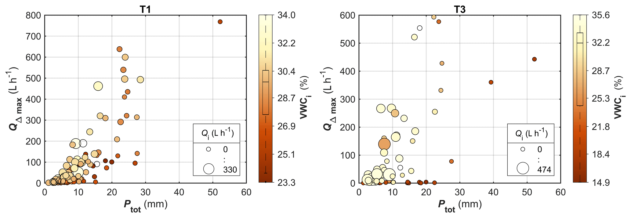
Figure 15 Relationship between Q_Δmax and P_tot as well as antecedent conditions (subevents and simple SSF events). The antecedent conditions are represented by VWC_i (colour of markers) and Q_i (size of markers). The boxplot in the colorbar describes the distribution of VWC_i.

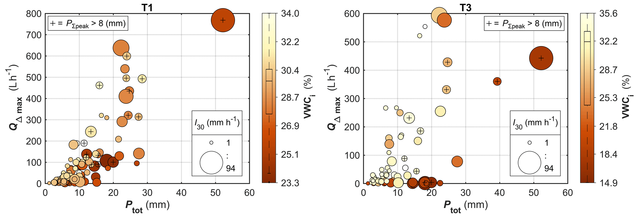
Figure 16 Relationship between Q_Δmax and P_tot as well as antecedent soil moisture conditions and I₃₀ (subevents and simple SSF events). Events were the cumulative rainfall calculated until peak rainfall intensity (I₅) is greater than 8 mm are marked with +. The size of the markers represents I₃₀ and the colour of the markers represents the VWC_i. The boxplot in the colorbar describes the distribution of VWC_i.

For SSF events associated with larger rainfall events (P_tot>20 mm), on the other hand, the initial conditions appeared to play a secondary role, as demonstrated by the extremely high Q_Δmax of events characterized by very dry initial conditions. For these larger events (P_tot>20 mm) rainfall intensity as well as the amount of rainfall preceding the peak 5 min rainfall intensity (P_Σpeak in Fig. 16) appeared to play a more important role. At both trenches the highest Q_Δmax values were associated with fairly high rainfall intensities. For example, at T1 the largest Q_Δmax was associated with a rainfall intensity I₃₀ of 94 mm h⁻¹ (I₅ of 247 mm h⁻¹) and very dry initial conditions, whereas at T3 the highest Q_Δmax was associated with an I₃₀ of 43 mm h⁻¹ (I₅ of 107 mm h⁻¹). For P_tot>20 mm, SSF events with $Q_{\mathrm{\Delta }max}>\mathrm{200}$ L h⁻¹ were generally associated with rainfall events with high I₃₀ (>18 mm h⁻¹) and/or with a rainfall amount preceding peak rainfall intensity exceeding 8 mm. Hence, the rainfall structure (i.e. temporal distribution of rainfall intensities) also showed to influence the SSF response. The results suggest that a combination of large P_tot, high intensities and/or large rainfall amounts preceding peak rainfall intensity was required to achieve very high Q_Δmax, while initial conditions played a subordinate role.

3.3.3 Rising rate, lag time and response time

The rising rate, calculated for sub- and simple SSF events, was positively correlated to P_tot as well as rainfall rate (Figs. 17 and 8). Especially events with extremely high rising rates were always associated with large P_tot and/or high rainfall intensities. Moreover, at T1, for example, SSF events associated with a similar P_tot of 22–24 mm showed rising rates ranging from ca. 15 to 1900 L h⁻², which can be explained by the associated I₆₀ ranging from 8 to 22 mm h⁻¹. The antecedent conditions, on the other hand, appeared to be less relevant. Nevertheless, some events with the highest rising rates were characterized by a low or a lack of initial trenchflow (see + in Fig. 17) and dry antecedent soil moisture conditions, suggesting that dry antecedent conditions do not hinder high rising rates but sometimes favour them. This is evident in the results of T1, where for events with similar P_tot, those characterized by dry initial conditions often exhibited higher rising rates than those with wetter initial conditions. At T3, the influence of the intensity and initial conditions was less evident, partly due to the smaller number of events with dry initial conditions (see boxplots in Fig. 17), as some events were excluded from the rising rate analysis (based on the criteria outlined in Sect. 2.3.5).

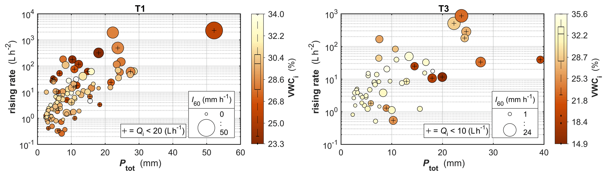
Figure 17 Relationship between rising rate and P_tot as well as antecedent conditions and I₆₀ (subevents and simple SSF events). The size of the markers represents I₆₀ and the colour of the markers represents the VWC_i. Events with Q_i<20 L h⁻¹ are marked with +. The boxplot in the colorbar describes the distribution of VWC_i. The y axis is logarithmic.

The time between centroid rainfall and peak flow (i.e. lag time) greatly varied for events with small rising rates, whereas it was mostly short for events with a high rising rate (Fig. 18). For example, the median lag time of events with a rising rate larger than 50 L h⁻² was 20 min (T1) and 85 min (T3), whereas it was 465 min (T1) and 328 min (T3) for smaller rising rates.

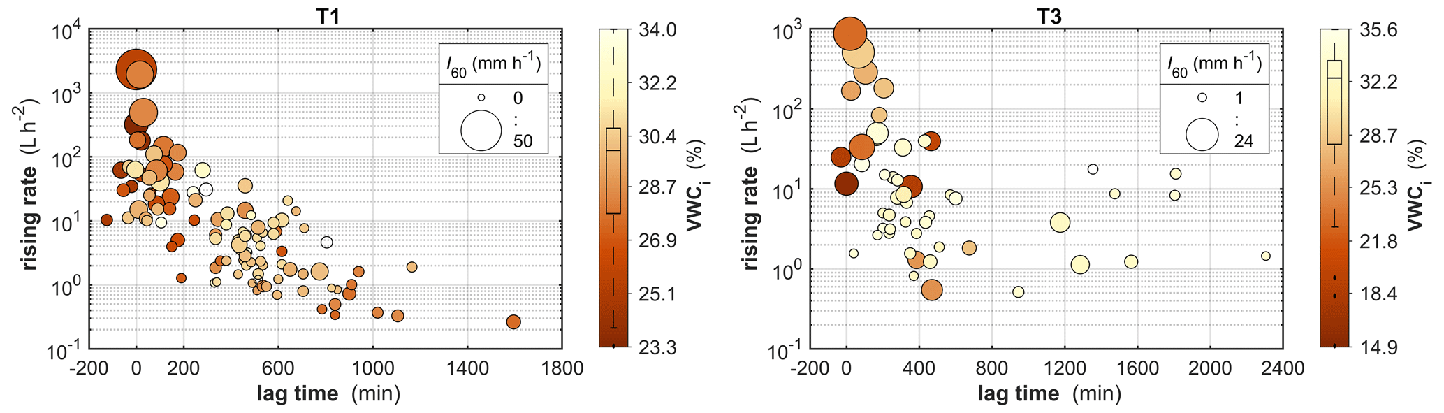
Figure 18 Relationship between rising rate and lag time as well as antecedent conditions and I₆₀ (subevents and simple SSF events). The size of the markers represents I₆₀ and the colour of the markers represents the VWC_i. The boxplot in the colorbar describes the distribution of VWC_i. The y axis is logarithmic.

The lag time, calculated for sub- and simple SSF events, was not sensitive to the size of the associated triggering rainfall event (P_tot) but was sensitive to its intensity (I₅ to I_m). Greater intensities were associated with smaller lag times. For example, at T1 the median I₆₀ of events with a lag time greater than 100 min was 2.4 mm h⁻¹, whereas for shorter lag times it was 6.6 mm h⁻¹. Similarly, at T3 the median I₆₀ was 2.5 and 6.5 mm h⁻¹, respectively. Dry initial conditions also seem to favour short lag times, as events with dry antecedent conditions generally exhibited short lag times. For example, at T1 the median lag time of events characterized by VWC_i and Q_i smaller than 26 % and 20 L h⁻¹ was 20 and 7 min, respectively, whereas for larger VWC_i and Q_i it was 460 and 490 min, respectively. T3 showed a similar pattern: the difference in the median lag time of events with VWC_i and Q_i smaller and larger than 26 % and 10 L h⁻¹, respectively, was 213 and 200 min, respectively.

The time between rainfall and SSF start can be calculated considering the rainfall centroid (i.e. response time, which is used in this analysis) as well as the start of the rainfall event. For both cases, their relationship to the rainfall event characteristics was found to be comparable. The P_tot as well as the cumulative rainfall calculated up to the SSF start showed to have a poor influence on the response time. Nevertheless, considering the cumulative rainfall up to SSF start, higher rainfall amounts were associated to a smaller variance in response time. Similar results were observed for the rainfall intensities preceding the SSF start, with variance decreasing as the intensities increase. These results indicate that a quick SSF response is more likely triggered by short, intense, and temporally focused rainfall events. The antecedent conditions did not show a clear relationship with the response time. Overall, the relationship between response time, rainfall event characteristics and antecedent conditions were not well defined.

3.3.4 Seasonality

To study the seasonality, the SSF and rainfall events were divided by season. For selected metrics the trimmed mean (i.e mean computed after excluding the lowest and highest 10 % of values) was calculated on a seasonal basis (see Fig. 19). The 95 % confidence intervals (CI) were computed for each trimmed mean using a bootstrap approach (1000 resamples, percentile method); they are presented in Appendix E. The VWC_i and I₃₀ associated to simple and complex events as well as non-triggering rainfall events showed a similar seasonal distribution as for the simple events and subevents and are thus not shown in Fig. 19. Overall, both trenches showed similar seasonal patterns. The seasonal means of V_tot and MCA were higher in winter and spring; however, the CI of these metrics are wide and partially overlap, hence seasonal differences require cautious interpretation. These high winter–spring means coincide with higher VWC_i (with comparatively narrow CI), and are therefore consistent with the expectation that wetter initial conditions reduce the rainfall input required to generate SSF. The P_tot was higher in spring than winter (at T1 the CI overlap). Nevertheless, the higher winter VWC_i seems to compensate for the smaller rainfall amounts. High Q_Δmax were observed in spring at both trenches and at T1 it was also relatively high during summer. At T3, Q_Δmax was moderate during summer despite the occurrence of relatively large and intense rainfall events, which is consistent with the dry initial conditions and their stronger influence on the SSF response at this site. The rising rate was highest in spring at T3 and in summer at T1, but with wide CI. The longest mean lag time was observed in spring at both trenches, and arises due to a handful of events with extremely long lag time, as reflected by the broad CI.

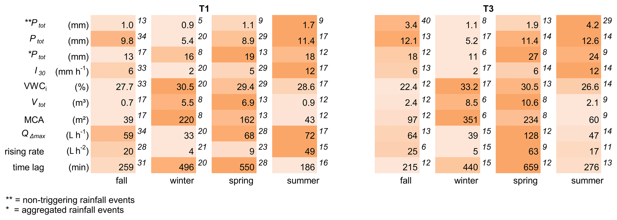
Figure 19 Seasonality of SSF and rainfall events characteristics. Values with a coloured background show the seasonal trimmed means, whereas the corresponding sample size (after trimming) is shown on a white background. For each metric, shading ranges from light to dark orange as values increase.

The total rainfall of non-triggering rainfall events (${}^{\ast \ast }{P}_{\text{tot}}$ in Fig. 19) also shows a seasonal trend. The highest and lowest ${}^{\ast \ast }{P}_{\text{tot}}$, observed during summer and winter months, respectively, are consistent with lower VWC_i in summer and higher VWC_i in winter as well as the change in interception storage (i.e. leafed and leafless periods). The same picture is given when the events are divided by growing (May–October) and dormant (November–April) season. Overall, the interception storage appears to be small (ca. <2–3 mm).

4 Discussion

4.1 Influence of total rainfall and antecedent conditions on contributing area and subsurface stormflow generation

The analysis has shown that at both trenches the event SSF volume (V_tot) is controlled by rainfall amount (P_tot) and antecedent wetness conditions (VWC_i and Q_i), with wet conditions producing one to three orders of magnitude larger events (V_tot) under similar P_tot (Figs. 9 and 10). These results are consistent with earlier studies reporting strong controls of rainfall amount and antecedent wetness on SSF volumes (e.g. Fu et al., 2013; Noguchi et al., 2001; Tromp-van Meerveld and McDonnell, 2006a). To account for the influence of the initial conditions on the generated stormflow volume, different authors have used the composite metric P_tot+ASI, which allowed to improve correlation strength and threshold detection (e.g. Detty and McGuire, 2010; Fu et al., 2013; Han et al., 2020; Zwartendijk et al., 2023). Nevertheless, ASI can over- or under-represent the initial soil moisture conditions in the composite metric P_tot+ASI, as it is highly dependent on the depth of the considered soil moisture profile; for the same soil moisture content, deeper profiles will yield higher ASI values, while shallower ones yield lower values. Therefore, as shown by Fu et al. (2013), the optimum depth to obtain the best fit can be site dependent. Hence, in this study we weighted the initially computed ASI in order to obtain the best fit to the datasets and explore the influence of the initial conditions. The observed higher correlation of V_tot vs. P_tot+ASI_adj than vs. P_tot (supported by CI_Δrs>0) highlights the considerable influence of the initial conditions on the total flow, and shows that the storage deficit, linked to drier antecedent conditions, was effectively accounted for using ASI_adj (see Fig. 8). The correlation increased by 0.1 (CI_Δrs 0.03–0.19) at T1 and by 0.2 (CI_Δrs 0.10–0.43) at T3 when including ASI_adj. The larger increase in correlation and the slightly higher weight at T3 indicates that the initial conditions have a higher influence at that site. This is also suggested by the on average larger rainfall amounts of the non-triggering rainfall events observed at T3 (Fig. 6).

Despite the importance of the antecedent conditions for SSF events associated with small to medium P_tot, the data shows that for SSF events associated with very large total rainfall depths (P_tot>50 mm) the influence of the antecedent conditions is often less pronounced and the P_tot–V_tot relationship is poor. These SSF events are characterized by a longer duration (>75th percentile) and multiple peaks (subevents). Thus, the subsurface has more time to drain between peaks and more water is lost by the consecutive rainfall events to replenish the storage deficit and during the transmission to the trench. The higher losses and inadequacy of considering only the wetness conditions at the start of these events are also reflected by the comparatively smaller MCA (Fig. 13) and poorer P_tot+ASI_adj vs. V_tot relationship. These results show the limitation of the applied approach for extremely large, long multi-peak SSF events. This finding matches the observations of Tromp-van Meerveld and McDonnell (2006a) where a poorer P_tot–V_tot relationship and a weaker influence of the initial conditions is seen for SSF events associated toP_tot>55 mm. Hrnčíř et al. (2010) also reported that for extremely large rainfall amounts (>70 mm) the initial conditions only exerted a smaller control on the total subsurface stormflow.

Regarding smaller events, at both trenches, the minimum P_tot to trigger a SSF response (activation threshold) under wet antecedent conditions was minimal, ranging between 2 and 3 mm, and was only slightly higher for dry antecedent conditions (Figs. 9 and 10). The results show that, although the initial conditions greatly influence V_tot, they are less relevant concerning the activation of SSF. Other hillslope-based studies have also shown that small rainfall amounts are sufficient to activate SSF. Noguchi et al. (2001) observed SSF generation for rainfall events as small as ∼5 mm under wet as well as dry antecedent conditions. Fu et al. (2013), who measured SSF at two plots, reported SSF events with minimum associated precipitation amounts of 12 and 14 mm, respectively. Moreover, Tromp-van Meerveld and McDonnell (2006a) showed that, although substantial SSF occurred only for precipitations amounts greater than 55 mm, much smaller amounts (<5 mm) were able to activate SSF.

At T1, beyond the SSF activation threshold of P_tot∼2 mm, especially events associated with wet antecedent conditions, show a nearly linear increase in V_tot with P_tot (Figs. 9 and 14). A similar linear increase, without any apparent further thresholds, was also observed at the catchment scale by Penna et al. (2011). In contrast, at T3, despite the general increase of V_tot with P_tot, V_tot appears to increase only weakly over the ranges of ca. 5–15 mm (wet antecedent conditions) and ca. 10–20 mm (dry antecedent conditions), and to rise steeply once P_tot exceeds ca. 15 mm (wet) and ca. 20 mm (dry; Figs. 10 and 14). However, we note that the scatter and the relatively small number of events in the aforementioned P_tot ranges imply substantial uncertainty. The 15 and 20 mm rainfall amounts can be interpreted as a second threshold beyond which significantly more SSF is generated. The observations at T3 match the results of most SSF studies (e.g. Du et al., 2016; Fu et al., 2013; Tani, 1997; Tromp-van Meerveld and McDonnell, 2006a), where such a sharp increase in V_tot was also observed once a precipitation threshold was exceeded. In the literature, the reported size of this second threshold, for the generation of significant SSF, under wet antecedent conditions ranges between 17–60 mm (Du et al., 2016; Graham et al., 2010; Mosley, 1979; Uchida et al., 2005; Weiler et al., 2006). Hence, our threshold of ca. 15 mm is located at the lower end of the spectrum of the reported values. Considering the composite variable P_tot+ASI_adj, the second threshold was at ca. 40 mm at T3 (Fig. 11). This suggests that significant SSF volumes can be generated by a relatively small rainfall event if the antecedent conditions are very wet (i.e. ASI_adj is close to 40 mm), whereas if the antecedent conditions are dry (ASI_adj≪40 mm) higher rainfall amounts are required to generate comparable SSF volumes. For example, a similar V_tot of 0.63–0.71 m³ resulted from a relatively small P_tot of 6 mm under wet initial conditions (ASI_adj ca. 37 mm), as well as from a large P_tot of 28 mm under dry initial conditions (ASI_adj ca. 17 mm). The initial conditions also influenced the MCA, as for similar P_tot the MCA was generally higher under wet antecedent conditions (Fig. 13). The strong fit of Eq. (4) suggests that the contributing area expands with P_tot, and the difference between events with wet and dry antecedent conditions indicates that the contributing area increases more rapidly with P_tot under wet than under dry conditions. For events with wet antecedent conditions, the quadratic coefficient a (Eq. 4) was significantly larger at T3 than at T1, implying a stronger rainfall dependence and a faster expansion of the contributing area at T3. The increase of the contributing area with P_tot is backed by field observations, which suggest that the contributing area can be much smaller than the maximum MCA. It was observed how for some smaller events at T1 and T3, the uppermost instrumented well located roughly 20 m above the trench did not show any reaction (i.e. no increase in water level), suggesting that for these cases the contributing area probably ended downslope of the well and was therefore smaller than the calculated maximum MCA. However, we cannot fully exclude that water could have laterally bypassed the uppermost well without producing a measurable response in the water level; hence, the contributing area may have extended upslope of the well despite the lack of a water level response. The increase in contributing area with storm size and wet antecedent conditions is in agreement with other studies at the hillslope scale (e.g. Šanda and Císlerová, 2009; Tromp-van Meerveld and McDonnell, 2006b, a) as well as at the catchment scale (e.g. Detty and McGuire, 2010; Zwartendijk et al., 2023). The dynamic nature of the subsurface contributing area and the difficulty of assessing it imply that converting the SSF volumes into equivalent water depths (i.e. mm), which requires the use of a fixed catchment area, can lead to unrepresentative and misleading values. However, assuming that the topographically derived catchment areas approximate the true catchment areas of the trenches, the ninefold larger area of T3 implies that, for the same SSF volume, the equivalent water depth (SSF depth) would be ∼9 times smaller at T3 than at T1. Consequently, the event with the greatest SSF depth would occur at T1, despite T3 having the event with the largest SSF volume. Hence, the larger SSF volumes observed at T3 are not necessarily linked to smaller losses (e.g. leakage into the bedrock) but could instead result from a larger area contributing to SSF, as suggested by the smaller max. subsurface runoff coefficient (C_sub) obtained for T3. Although the assumed topographic catchment area influences the absolute values of V_tot and Q_Δmax when expressed in mm and mm h⁻¹, respectively, it does not alter the trench-specific patterns observed between SSF, rainfall, and antecedent conditions metrics.

Our findings support that, for small events, especially if characterized by dry antecedent conditions, the contributing area tends to be small, as an expansion further upslope is likely restricted by transmission losses (i.e. leakage through the impeding layer) and/or storage deficits (i.e. “storage barriers”), which are overcome during larger precipitation events. Studies have shown that these storage barriers can result, among other factors, from the spatial variation of soil thickness, the topography of the impeding layer (i.e. depression storage) and the vertical variation in hydraulic conductivity, which controls the leakage rate through the impeding layer as well as the possible onset of faster lateral flow within upper more permeable layers (McGuire et al., 2024). Moreover, low soil moisture levels represent an additional barrier that needs to be overcome (Penna et al., 2011). These barriers can increase gradually or abruptly, as suggested by the gradual and sharper increase of V_tot as well as MCA with P_tot observed at T1 and T3, respectively (Figs. 9, 10 and 13). At T3, the phase of markedly reduced increase of V_tot with P_tot between ca. 5–15 mm (wet antecedent conditions) and 10–20 mm (dry antecedent conditions) suggests that, at this site, a storage barrier of ca. 10 mm prevents further expansion of the contributing area (see Fig. 10). This barrier, which appears to be present during wet and dry initial conditions, may be the result of depressions on the irregular bedrock topography, which have to be filled before any significant lateral flow originating from areas further upslope can occur (fill and spill mechanism). This is supported by the steep topography and spatial distribution of the outcrops observed in the field. Nevertheless, other mechanisms cannot be ruled out, and we acknowledge that the small number of events within the reported P_tot ranges limits the robustness of this interpretation. Compared with other study sites where flow over an impeding layer (e.g. bedrock) is the dominant SSF-producing mechanism, the second threshold of 15–20 mm (wet–dry conditions) observed at T3 is similar to the 17 and 20 mm thresholds reported for the Maimai and Tatsunokuchi-yama hillslopes, respectively (Graham et al., 2010; Tani, 1997). However, it is much smaller than the 55 mm threshold observed at Panola (Tromp-van Meerveld and McDonnell, 2006a) and the 60 mm threshold reported for a hillslope at the Savannah River Site (SRS) by Du et al. (2016). These threshold differences are broadly consistent with differences in hillslope gradient. T3, Maimai and Tatsunokuchi-yama have relatively steep average slopes of 27, 29 and 35°, respectively, compared with 13° at Panola and 4° at the SRS hillslope. As proposed by Graham et al. (2010), who compared the response of Maimai and Panola, steeper bedrock gradients may reduce the storage capacity of bedrock depressions because, assuming similar bedrock surface roughness, less water is required to fill depressions before spill and lateral connectivity occur. This provides a plausible explanation for the relatively low threshold observed at T3. However, other factors such as the site-specific bedrock topography, the soil thickness, the permeabilities of the soil and impeding layer, and the permeability contrast between them can also control the threshold (Graham et al., 2010; Hopp and McDonnell, 2009).

At T1 the continuous baseflow and shallow water table suggest that at the site SSF is generated by the water table rising into a more permeable zone near the surface (transmissivity feedback mechanism). Thus, the gradual increase of V_tot with P_tot can be explained by a gradual increase in storage losses and/or vertical losses further upslope. The bedrock was not reached by the ∼3 m deep trench, suggesting that its influence on the SSF dynamics at T1 is smaller than at T3.

4.2 Controls on peakflow

Our results show that Q_Δmax is mainly controlled by P_tot and antecedent soil moisture conditions (VWC_i) for SSF events associated with rainfall events smaller than approximately 20 mm (Fig. 15). Whereas for SSF events associated with larger rainfall amounts, while P_tot is still important, the initial conditions play a subordinate role and rainfall intensity as well as the amount of rainfall preceding peak rainfall intensity (P_Σpeak) appear to be important factors. The switch from initial conditions to rainfall intensities and/or P_Σpeak as controlling factors is not abrupt but gradual, especially at T1 where the influence of the initial conditions is less pronounced than at T3. The strong influence of the initial conditions on Q_Δmax is reflected by the increase in correlation (corroborated by CI_Δrs) when ASI_adj is added to P_tot (see Fig. 8). The increase and the adjustment factor of ASI (i.e. weight of the ASI) are particularly high at T3, supporting the larger influence of the initial conditions at the site. The relatively weak (T1) and extremely weak (T3) correlation coefficients between Q_Δmax and the rainfall intensities confirm that the intensities alone are not sufficient to explain Q_Δmax. The somewhat higher values observed for T1 can be explained by the combined effect of the higher V_tot–P_tot correlation and the correlation present between P_tot and the rainfall intensities. Moreover, at T1 the smaller influence of the antecedent soil moisture conditions suggests a smaller soil moisture storage, which being more easily filled up allows the rainfall intensity to exert a larger influence. The stronger influence of the initial conditions observed for SSF events associated with smaller rainfall events can be explained by the larger fraction of water lost to fill the storage deficit of the soil. Only when the storage is filled and the contributing area is large are higher rainfall rates able to generate and sustain higher subsurface flowrates, and thus exert a larger control on Q_Δmax. This is also backed by the higher Q_Δmax generated by rainfall events with moderate I₃₀ but high precipitation amounts preceding peak rainfall.

Other authors observed similar relationships between peakflow, storm size, rainfall intensities and antecedent conditions. Noguchi et al. (2001) documented an increase in subsurface peakflow with I₃₀ for events with wet conditions, while during dry conditions the relationship was less strong and only present for part of the observed trenchface. Hrnčíř et al. (2010) also found that the initial soil moisture had a major control on the subsurface peakflow. Moreover, Fu et al. (2013) observed that beyond a threshold of I₃₀ of ca. 6 and 12 mm h⁻¹ (two trenches) the I₃₀ correlated to the subsurface peakflow. However, two events with high antecedent soil moisture showed high peakflows even with low I₃₀ (below threshold). At the catchment scale, Zwartendijk et al. (2023) observed how peakflow was highly correlated to P_tot+ASI as well as with V_tot and that while peakflow was also influenced by I₆₀ the P_tot and antecedent conditions where the major controlling factors. These studies suggest that, like at our trench sites, rainfall intensity has a lower influence under dry initial conditions but once the storage deficit is filled and the contributing area is large high rainfall intensities can generate high trenchflow rates especially when associated with large P_tot.

4.3 Timing and rising rate

Our findings show how the rising rate is positively correlated to P_tot as well as rainfall rate (I_m, I₅, I₃₀ and I₆₀) (Figs. 17 and 8). The relationship with P_tot is roughly exponential, although the scatter is relatively large in part due to the different rainfall intensities. Dry initial conditions seem to not hinder the generation of steep rising limbs but, in some instances, to favour it (observed at T1 but not at T3).

The lag time (centroid rainfall–peakflow) is short for events with high rising rates but greatly varies for events with lower rising rates, resulting in a negative correlation between rising rate and lag time (Figs. 8 and 18). Similar results were found when the time between peak rainfall and peakflow was considered. The link between short lag times and steep rising limbs suggest that short travel times reduce the dispersion of the rainfall pulse traveling through the subsurface allowing for a sharper increase in discharge.

The lag time was found to be not correlated to the size of the rainfall event but to its intensity. The correlation between lag time and intensities is negative (see Fig. 8), with the lag time variability decreasing as rainfall intensities increase. For example, at T1 and T3 SSF events associated with rainfall events with I₃₀ exceeding 15 mm h⁻¹ had a standard deviation of the lag time seven and four times smaller than events with lower intensity, respectively. At the catchment scale, similar observations were made by Zhang et at. (2021). Knapp et al. (2025), also found that the lag time was shortened by higher precipitation intensities and was largely unaffected by antecedent wetness conditions. Our observations also align with the findings of Han et al. (2020), as they report that the time required to generate connectivity in the hillslope-riparian-stream system, and hence produce significant runoff, was related to the peak rainfall intensity (I₃₀), but not the accumulated rainfall amount. Moreover, they observed how dry initial conditions can favour connectivity within the catchment. In agreement, we found that short lag times were often associated with dry initial conditions. Shorter lag times were also associated with smaller MCA (Fig. 8), especially under dry antecedent conditions. Similarly, Haga et al. (2005) observed how, at the catchment scale, the lag time increased with the increasing source area.

Our results suggest that dry conditions can favour preferential flow, which allows the pulse to travel more quickly through the subsurface bypassing the dry matrix. Evidence of preferential flow in our study catchment was found by Pyschik and Weiler (2026). Furthermore, dry conditions were linked to smaller MCA and thus shorter flow paths, which in turn promote a shorter travel time and hence smaller lag times. The reduced lag time linked to higher intensities can also be explained by the associated faster wetting (assuming rainfall intensity < infiltration capacity) and thus a quicker arrival of the main rainfall pulse to the trench.

The response time (centroid rainfall–start SSF) showed to be poorly related to P_tot as well as to the cumulative rainfall calculated up to the start of the SSF event. Nevertheless, the variability in response time shows a decrease with increasing rainfall amounts preceding the SSF start. Similarly, higher rainfall intensities were associated with a lower variance in response time. Overall, the relationship between response time, rainfall event characteristics and antecedent conditions is not well defined. Comparable (short) response times occurred under different combinations of rainfall characteristics and antecedent wetness. For example, events with low intensities and small rainfall amounts produced responses that were as fast as those of large and intense rainfall events under dry conditions, indicating that response time is not uniquely determined by rainfall amount or intensity. Moreover, short response times were occasionally observed even for events with small rainfall amounts under dry antecedent conditions. The timing of SSF can be controlled by a multitude of factors (e.g. soil depth, bedrock topography, macropore and preferential flow network, slope, permeability contrast) whose relevance can change depending on antecedent conditions, rainfall characteristics and SSF-producing mechanism (e.g. saturated flow over impeding layer, macropore flow, flow in higher permeability zone) (McGuire et al., 2024). Besides these complexities, the way the response time is defined can also lead to a large variation in response times. For example, the time can be calculated from the centroid or the peak rainfall, which in turn are influenced by the method and thresholds (e.g. MIT 6 h) used to define the rainfall events, but also by the particular structure of the rainfall events. Using the start of the rainfall event is also problematic, as the time will be highly influenced by the rainfall structure. The result is that only a handful of authors have studied the response time and its relationship with rainfall as well as hillslope/catchment characteristics. The large range in the response time and its variability within the hillslope was documented by Freer et al. (2002), who, for example, described how a certain trench section responded ca. 4 times slower than the fastest one. An even higher variability was found at the catchment scale in the study of Zwartendijk et al. (2023), who also observed that the response time (start rainfall to start stormflow) was poorly to not significantly correlated to the antecedent conditions.

4.4 Seasonal variation of SSF

The results showed a marked seasonal variation of the SSF response (Fig. 19). The observed pattern can be linked to the seasonal variation of the rainfall characteristics and antecedent conditions, which ultimately control the SSF response. For instance, the great V_tot and MCA in winter and spring can be explained by the combined high precipitation amounts and wet initial conditions. Similarly, at the catchment scale, Penna et al. (2015) reported a strong seasonal variability in runoff responses related to antecedent moisture conditions and rainfall event size, with runoff coefficients being markedly higher in spring than in summer. Sidle et al. (1995) documented greater runoff coefficients during the wet season, which in combination with larger precipitation events, produced greater SSF volumes at the hillslope scale. Likewise, Tromp-van Meerveld and McDonnell (2006a) reported greater trenchflow runoff coefficients in winter than in summer. Blume et al. (2009) observed shorter response times for streamflow in summer compared to winter, consistent with our findings of much smaller lag times in summer compared to the wetter winter and spring.

Given the relevance of the antecedent wetness conditions, many SSF studies simply divide the dataset into wet and dry periods or into growing (typically dry) and dormant (typically wet) seasons (e.g. Detty and McGuire, 2010; Sidle et al., 1995). However, the seasonal variability in SSF is rarely examined explicitly, as most SSF studies are based on short observation periods and thus only cover a limited number of events. Our study highlights the importance of investigating SSF over extended time periods in order to capture the responses across seasons and, ultimately, a wide range of rainfall characteristics and antecedent conditions.

5 Conclusions

In our study, subsurface stormflow (SSF) volume was primarily controlled by total rainfall and antecedent wetness conditions, with wet initial conditions yielding up to three orders of magnitude more volume. Our data suggest that the observed increase in event SSF volume with total rainfall is associated with an expansion of the contributing area, as indicated by the increase in the minimum contributing area. Peakflow was mainly controlled by total rainfall and initial wetness conditions for small rainfall events, whereas for larger events the influence of the initial conditions diminished, and rainfall intensity as well as rainstorm structure became more important controlling factors. Steep rising limbs were related with short response times and occurred under higher rainfall amounts and intensities. Using a weighted antecedent soil moisture index (ASI) in the combined variable total rainfall + ASI helped to quantify the influence of initial soil moisture conditions relative to the total rainfall on the different SSF response metrics.

Our results highlight the complex interactions between rainfall characteristics, antecedent wetness conditions and SSF responses, which could only be captured by analysing many events across seasons, underscoring the importance of long observation periods. The rapid SSF response and the large volumes and flow rates observed at our 11–14 m wide trenches, coupled with their proximity to the stream, suggest that SSF can substantially contribute to streamflow. Thus, our findings can serve both as a benchmark to verify hillslope-scale hydrological models and as a proxy for predicting the occurrence and magnitude of SSF in catchment-scale models. Further studies at the trench sites focusing on the inter-event dynamics of soil moisture, water level, trenchflow and its partitioning as well as artificial rainfall experiments will help to shed more light on the complex processes controlling SSF at the hillslope scale.

Appendix A

Figure A1 Trenches during construction.

Appendix B

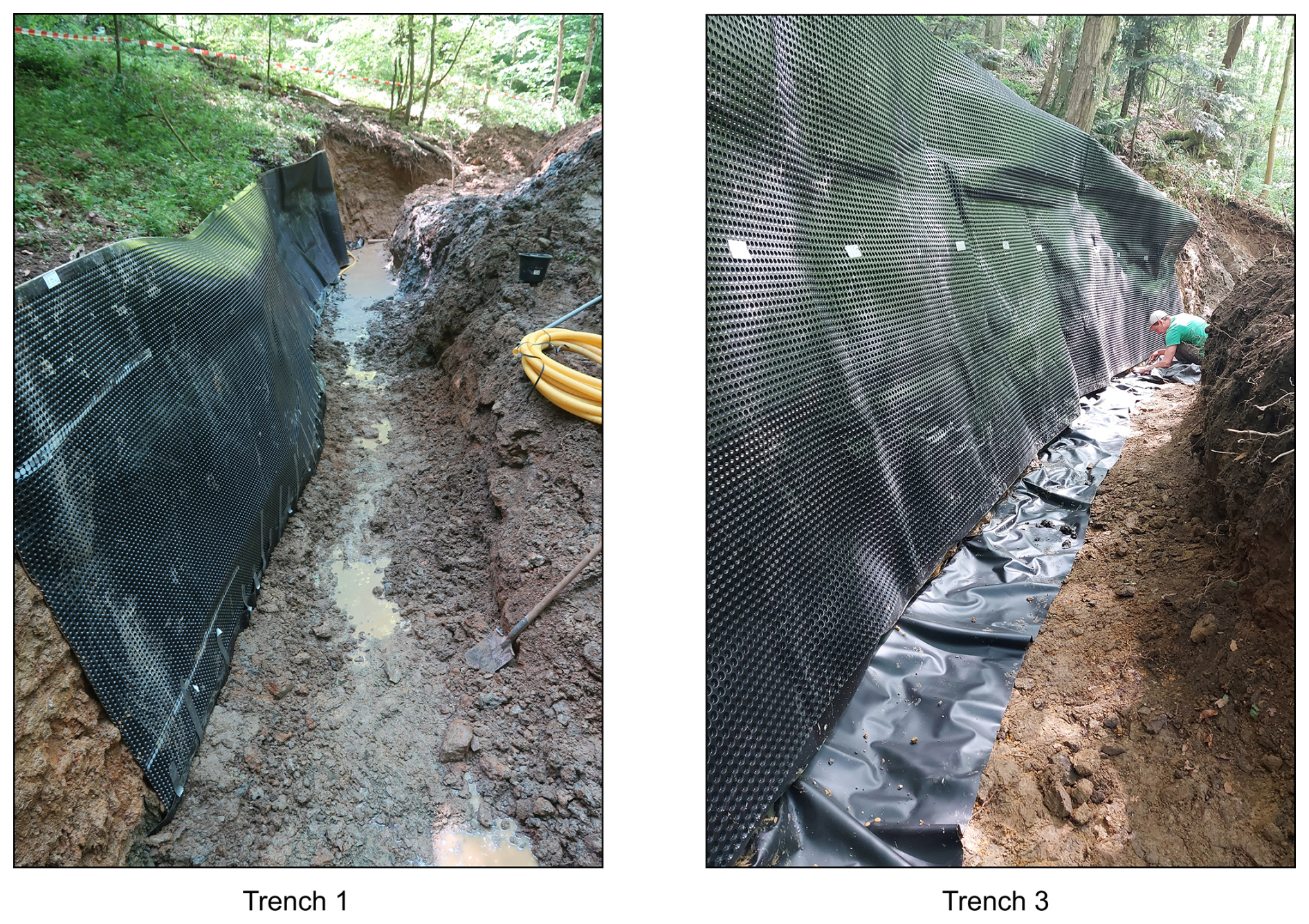
The volumetric water content (VWC) was derived from the dielectric permittivity and temperature data using the Complex Refraction Index Model (CRIM) (Eq. B1) which accounts for the individual permittivities of air (K_air), solid (K_s) and water (K_water) (Roth et al., 1990). In the equation, K_a is the measured (apparent) dielectric permittivity while n and β are the porosity and shape factor, respectively.

$$\begin{array}{}\text{(B1)}& \text{VWC}=\mathrm{100}\times {\displaystyle \frac{K_{\mathrm{a}}^{\mathit{\beta }}-(\mathrm{1}-n)\times K_{\mathrm{s}}^{\mathit{\beta }}-n{K}_{\text{air}}^{\mathit{\beta }}}{K_{\text{water}}(T{)}^{\mathit{\beta }}-K_{\text{air}}^{\mathit{\beta }}}}\end{array}$$

While the effect of temperature on K_air and K_s is negligible, on K_water it is not (Wraith and Or, 1999). Therefore, if temperature is not accounted for when calculating the VWC (e.g. using the Topp equation; Topp et al., 1980), diurnal temperature cycles and seasonal temperature variations can lead to erroneous VWC values. This was avoided by applying the CRIM with a temperature-corrected K_water. The temperature dependence of K_water was taken into account using Eq. (B2) (Weast, 1986); where T° is the temperature in degree Celsius.

$$\begin{array}{}\text{(B2)}& \begin{array}{rl}{K}_{\text{water}}& =\mathrm{78.54}\times \\ [& \mathrm{1}-\mathrm{4.579}\times {\mathrm{10}}^{-\mathrm{3}}(T\mathit{°}-\mathrm{25})\\ & +\mathrm{1.19}\times {\mathrm{10}}^{-\mathrm{5}}(T\mathit{°}-\mathrm{25}{)}^{\mathrm{2}}\\ & -\mathrm{2.8}\times {\mathrm{10}}^{-\mathrm{8}}(T\mathit{°}-\mathrm{25}{)}^{\mathrm{3}}]\end{array}\end{array}$$

Nevertheless, an accurate temperature-corrected VWC can only be obtained if the CRIM-variables porosity (n), K_s and β are reasonably well known, as those variables have a considerable influence on the resulting VWC. Hence, by applying the CRIM the temperature effect can be accounted for but the uncertainty on the absolute VWC values is related to the uncertainty of K_s and, more importantly, porosity (n).

In this study, K_s was assumed to be 4, since for mineral soils it typically ranges between 3 and 5 (Behari, 2005; Chan and Knight, 1999; Kirsch, 2009). A β of 0.5 was used, as this is the most commonly used value (Zadhoush et al., 2021), and K_air was set to 1. Where available, the porosity measured in the lab (from fitted water retention curve obtained from HYPROP 2 and WP4C (METER-Group) measurements) for the undisturbed soil samples taken near the sensor location was considered. However, soil samples were only collected along the deepest soil moisture profile (S3), thus for the shallower profiles (S1 and S2) the porosities were estimated based on the one measured at S3. The lab-measured porosities were adjusted when the max. VWC resulting from the Topp and from the CRIM equation (computed using the original lab-measured porosities) were substantially higher than the measured porosities (e.g. 41 % vs. 25 % for the 2 m b.g.l. sensor at T3 S3; see Table B1). Since VWC values greater than the porosity do not make physically sense, the porosity was adjusted using the max. observed VWC (Topp) as a guideline and ensuring that the max. CRIM-calculated VWC approximated the adjusted porosity, under the assumption that during saturated or near-saturated conditions the VWC approximates porosity. The porosities used for the final calculation are shown in Table A1. Differences between lab-measured porosities and those used to calculate soil moisture with the CRIM approach may result from spatial offsets between sampling and sensor locations, small-scale heterogeneity, and installation-related disturbance in gravel-rich deposits, which may locally modify the porosity within the sensor's measurement volume.

Table B1 Porosity at the sensor's location used to calculate the soil moisture (CRIM).

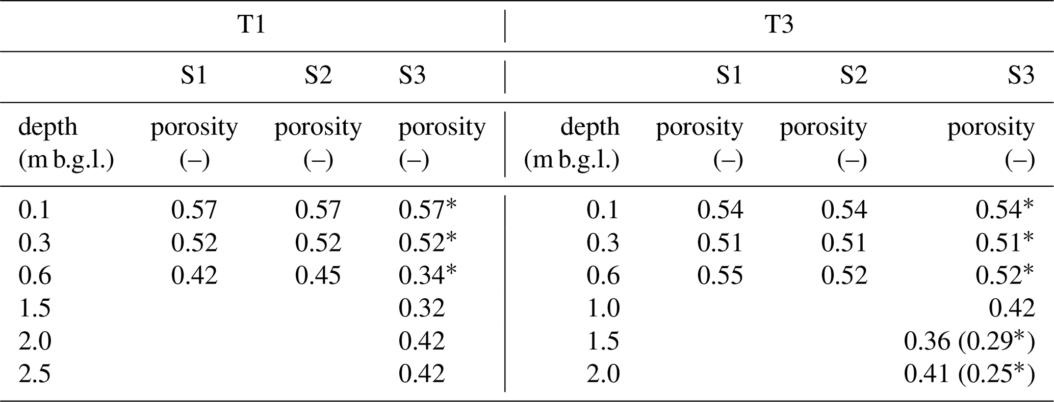
^∗ = lab-measured porosities
(not used porosity).

Appendix C

The SSF events were delineated using a semi-automatic method developed within this study. In the following, the method is described in detail, including inputs, outputs, implemented steps and variables involved.

The rainfall timeseries must have a temporal resolution of 5 or 10 min and be previously separated into events (see Sect. 2.3.2 Rainfall event delineation), as the start and end of the events serve as input. The trenchflow record must have, or be resampled to, a time resolution of 10 min. The method was written using MATLAB (The MathWorks Inc, 2021) and the commented sourcecode is available upon request.

The flowchart in Fig. C1, outlines the steps taken to detect the start and end points of the events, whereas Figs. C2 and C3 further illustrate the moving windows and criteria used in the process. The start is detected as follows:

• 1.

  The time series is scanned from the start to the end + 6 h of every rainfall event to evaluate if an “unusual” increase in discharge (Q), which indicates the start of an SSF event, occurs. Six hours are chosen due to the defined MIT of 6 h.

• 2.

  During the scan, it is tested if baseflow, computed using a 5 h backward moving average ($\stackrel{\mathrm{‾}}{Q_B}$) of the trenchflow rate (Q) (i.e. arithmetic average between Q_i and Q_{i−300 min}), is present. This is:

  $$\begin{array}{}\text{(C1)}& {\stackrel{\mathrm{‾}}{Q_B}}_{\mathrm{i}-\mathrm{10}\min }>\mathrm{0}\end{array}$$
• 3.

  If no baseflow is detected, the algorithm tests the time series for flow onset; this is:

  $$\begin{array}{}\text{(C2)}& Q_{\mathrm{i}}>\mathrm{0}\end{array}$$

  • If an increase is found, the position is marked as the start of a new event and the scanning stops;

  • else, the scanning continues up to the end of the rainfall event + 6 h.

• 4.

  If baseflow is present, the code evaluates if there is any significant (i.e. “unusual”) increase in discharge by: calculating short (10 min) and long (60 min) forward moving averages ($\stackrel{\mathrm{‾}}{Q_{FS}}$ and $\stackrel{\mathrm{‾}}{Q_{FL}}$) (i.e. arithmetic average from Q_i to Q_i+10 min and Q_i to Q_i+60 min, respectively), computing the differences between $\stackrel{\mathrm{‾}}{Q_B}$ of the previous timestep and $\stackrel{\mathrm{‾}}{Q_{FS}}$ as well as $\stackrel{\mathrm{‾}}{Q_{FL}}$

  $$\begin{array}{}\text{(C3)}& {\displaystyle }\mathrm{\Delta }{Q}_{S_{\mathrm{i}}}={\stackrel{\mathrm{‾}}{Q_{FS}}}_{\mathrm{i}}-{\stackrel{\mathrm{‾}}{Q_B}}_{\mathrm{i}-\mathrm{10}\min }\text{(C4)}& {\displaystyle }\mathrm{\Delta }{Q}_{L_{\mathrm{i}}}={\stackrel{\mathrm{‾}}{Q_{FL}}}_{\mathrm{i}}-{\stackrel{\mathrm{‾}}{Q_B}}_{\mathrm{i}-\mathrm{10}\min }\end{array}$$

  and evaluating if ΔQ_S and ΔQ_L are both above a certain threshold Q_T

  $$\begin{array}{}\text{(C5)}& \left\{\begin{array}{l}\mathrm{\Delta }{Q}_{S_{\mathrm{i}}}>Q_T\\ \mathrm{\Delta }{Q}_{L_{\mathrm{i}}}>Q_T\end{array}\right.\end{array}$$

  as well as testing if

  $$\begin{array}{}\text{(C6)}& Q_{\mathrm{i}}-{\stackrel{\mathrm{‾}}{Q_B}}_{\mathrm{i}-\mathrm{10}\min }>\left({\displaystyle \frac{Q_T}{\mathrm{2}}}\right).\end{array}$$

  The latter avoids that the start is defined one timestep too early (i.e. in cases where Q_i is similar to ${\stackrel{\mathrm{‾}}{Q_B}}_{\mathrm{i}-\mathrm{10}\min }$ but due to the high value of Q_i+10 min the criterion in Eq. C5 is fulfilled), as the start has to coincide with the “unusual” increase in Q.

  • If the above criteria (Eqs. C5 and C6) are not fulfilled the scanning continues;

  • else, the time step is marked as the start of a new event and the scanning stops.

  Once the starting points of the events are defined, the ending points, which have to be followed by an “uneventful” period (i.e. a period associated with negligible changes), are detected as follows:

• 5.

  The time series is scanned from each previously detected starting point.

• 6.

  The change of the smoothed discharge ($\stackrel{\mathrm{‾}}{Q_C}$), calculated using an 80 min centered moving average (i.e. arithmetic average between Q_i−40 min and Q_i+40 min), is computed over a 4 h period ($\mathrm{\Delta }\stackrel{\mathrm{‾}}{Q_C}={\stackrel{\mathrm{‾}}{Q_C}}_{\mathrm{i}+\mathrm{240}\min }-{\stackrel{\mathrm{‾}}{Q_C}}_{\mathrm{i}}$). The time series of differences $\mathrm{\Delta }\stackrel{\mathrm{‾}}{Q_C}$ is then further smoothed using a 20 min centered average approach (resulting in $\stackrel{\mathrm{‾}}{\mathrm{\Delta }{Q}_C}$). Next, the standard deviation of $\stackrel{\mathrm{‾}}{\mathrm{\Delta }{Q}_C}$ is calculated over a 4 h forward window (i.e. $\mathit{\sigma }\stackrel{\mathrm{‾}}{\mathrm{\Delta }{Q}_C}$ is equal to the sd. between ${\stackrel{\mathrm{‾}}{\mathrm{\Delta }{Q}_C}}_{\mathrm{i}}$ and ${\stackrel{\mathrm{‾}}{\mathrm{\Delta }{Q}_C}}_{\mathrm{i}+\mathrm{240}\min }$). Finally, the end of an event is marked when the following three criteria are fulfilled:

  $$\begin{array}{}\text{(C7)}& \left\{\begin{array}{l}{\stackrel{\mathrm{‾}}{\mathrm{\Delta }{Q}_C}}_{\text{min}}\le {\stackrel{\mathrm{‾}}{\mathrm{\Delta }{Q}_C}}_{\mathrm{i}}\le {\stackrel{\mathrm{‾}}{\mathrm{\Delta }{Q}_C}}_{\text{max}}\\ \mathit{\sigma }{\stackrel{\mathrm{‾}}{\mathrm{\Delta }{Q}_C}}_{\mathrm{i}}<{\mathit{\sigma }}_T\\ {\stackrel{\mathrm{‾}}{Q_C}}_{\mathrm{i}}<({\stackrel{\mathrm{‾}}{Q_B}}_{\text{start}-\mathrm{10}\min }+Q_T)\end{array}\right.\end{array}$$

  where ${\stackrel{\mathrm{‾}}{\mathrm{\Delta }{Q}_C}}_{\text{min}}$ and ${\stackrel{\mathrm{‾}}{\mathrm{\Delta }{Q}_C}}_{\text{max}}$ are threshold-values that limit the acceptable change in the discharge over the next 4 h, while the threshold σ_T quantifies the acceptable variation of the discharge withing the same 4 h period. Setting low threshold values ensures that in the period following potential ending points Q does not increase nor decrease substantially. Low σ_T values in particular help to discard periods with fast-changing Q and to detect periods with well-defined trends. Due to the methodology a period of ca. 4 h from every timestep is analysed. To avoid that high “plateaus” within an event are erroneously detected as ending points the discharge value ($\stackrel{\mathrm{‾}}{Q_C}$) of the ending point has to be lower than the baseflow at the start of the event $\left({\stackrel{\mathrm{‾}}{Q_B}}_{\text{start}-\mathrm{10}\min }\right)+Q_T$ (threshold also used for the start detection) (i.e. it has to be less than Q_T above the baseflow). The addition of Q_T avoids that extremely shallow recession limbs hinder the detection of event ends within a reasonable time and that new slightly higher baseflows are not readily discarded for the placement of an ending point.

• 7.

  Lastly, because the average-based method makes it difficult to pinpoint the end of an event when Q alternates between flow and no-flow conditions, the code scans backwards from the detected end point until Q is greater than zero. Once the condition is met, the endpoint is moved in front of the identified non-zero Q time step.

The above-described method was applied to the measured trenchflows using following parameters: Q_T=1.0 L h⁻¹, σ_T=0.5 L h⁻¹, ${\stackrel{\mathrm{‾}}{\mathrm{\Delta }{Q}_C}}_{\text{max}}=\mathrm{0.3}$ L h⁻¹ and ${\stackrel{\mathrm{‾}}{\mathrm{\Delta }{Q}_C}}_{\text{min}}=-\mathrm{0.05}$ L h⁻¹. The chosen values obviously affect the number as well as the placement of the detected starting and ending points. Therefore, they have to be carefully selected according to the observed trenchflow signal. The optimal value of Q_T and σ_T will depend, among other things, on the resolution of the flow gauge and on the amplitude of the signal noise. In this study the flow was measured using tipping bucket systems. Therefore, Q_T and σ_T were related to the flow equivalent to 1 tip per 10 min which equalled to ca. 0.5 L h⁻¹.

The delineation results showed that most of the detected starts and ends of the events appear, after a visual inspection, at acceptable locations. Nevertheless, a small portion of them was placed at inappropriate locations. In fact, the method struggles to correctly locate the start when the increase in Q is very small and of similar magnitude as the signal noise, or when the start of a new event occurs during the steep recession phase of the preceding event. The latter arises due to the 5 h backward time window used to compute the “baseflow”, as higher discharge values of the falling limb would then also be included in the time window. Misplacements of ending points, on the other hand, can arise when the recession is more noisy than usual or when the new baseflow is considerably higher than the one preceding the event.

Hence, after the automatic delineation, the results had to be manually checked and were modified if necessary. This meant adding or removing a starting point as well as adjusting the position of starting and ending points. For this reason, the method is considered to be semi-automatic. To get an idea on the performance, for T1 and T3 on average ca. 4 % of the starts had to be added, 15 % had to be removed and 12 % of the starts had to be re-positioned, while 21 % of the ends had to be re-positioned.

The mentioned lengths of the periods used to calculate the averages, differences, etc., were chosen to best fit the analysed trenchflow data. Nevertheless, for different scales and other hydrological and hydrogeological settings the lengths of these periods could be adjusted.

Figure C1 Flow chart of the subsurface stormflow event delineation method.

Figure C2 SSF start detection method when baseflow is present.

Figure C3 SSF end detection method.

Appendix D

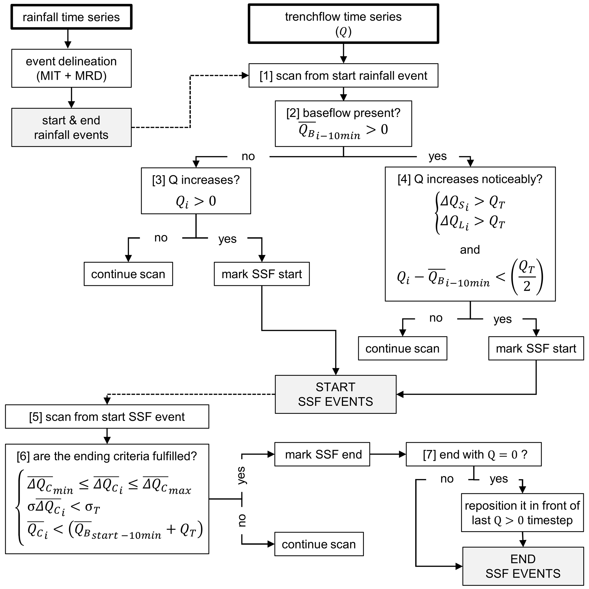
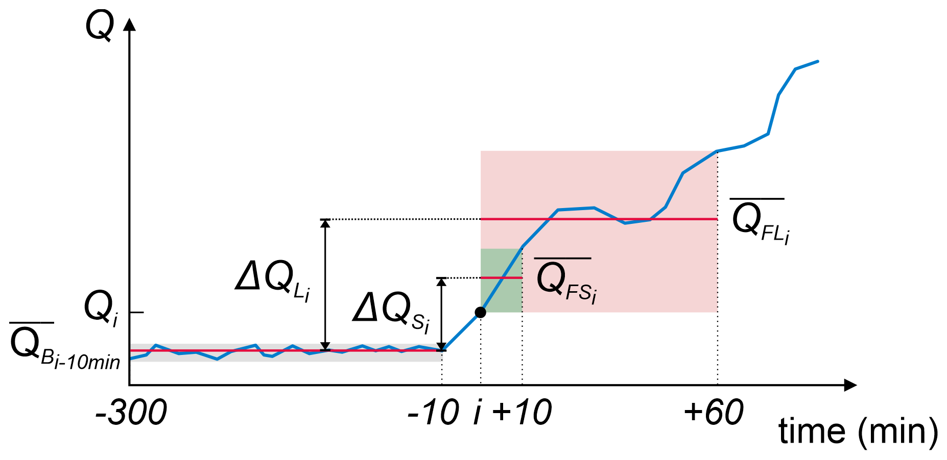
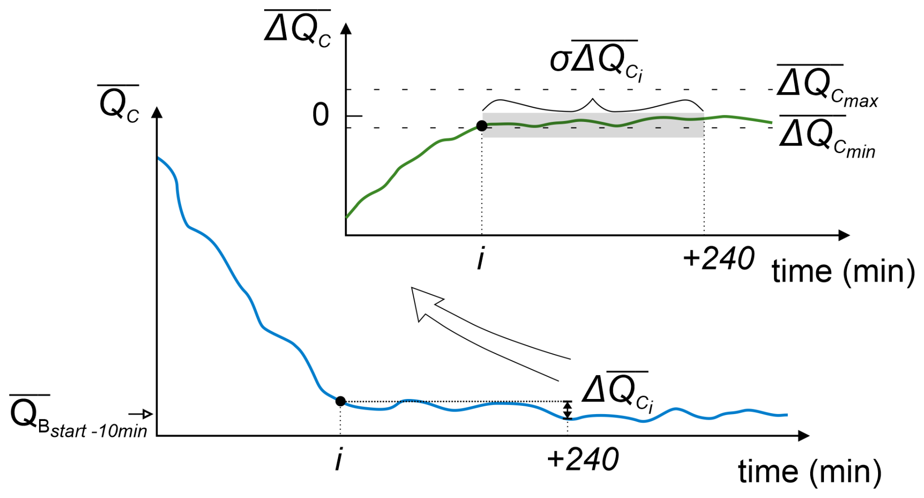
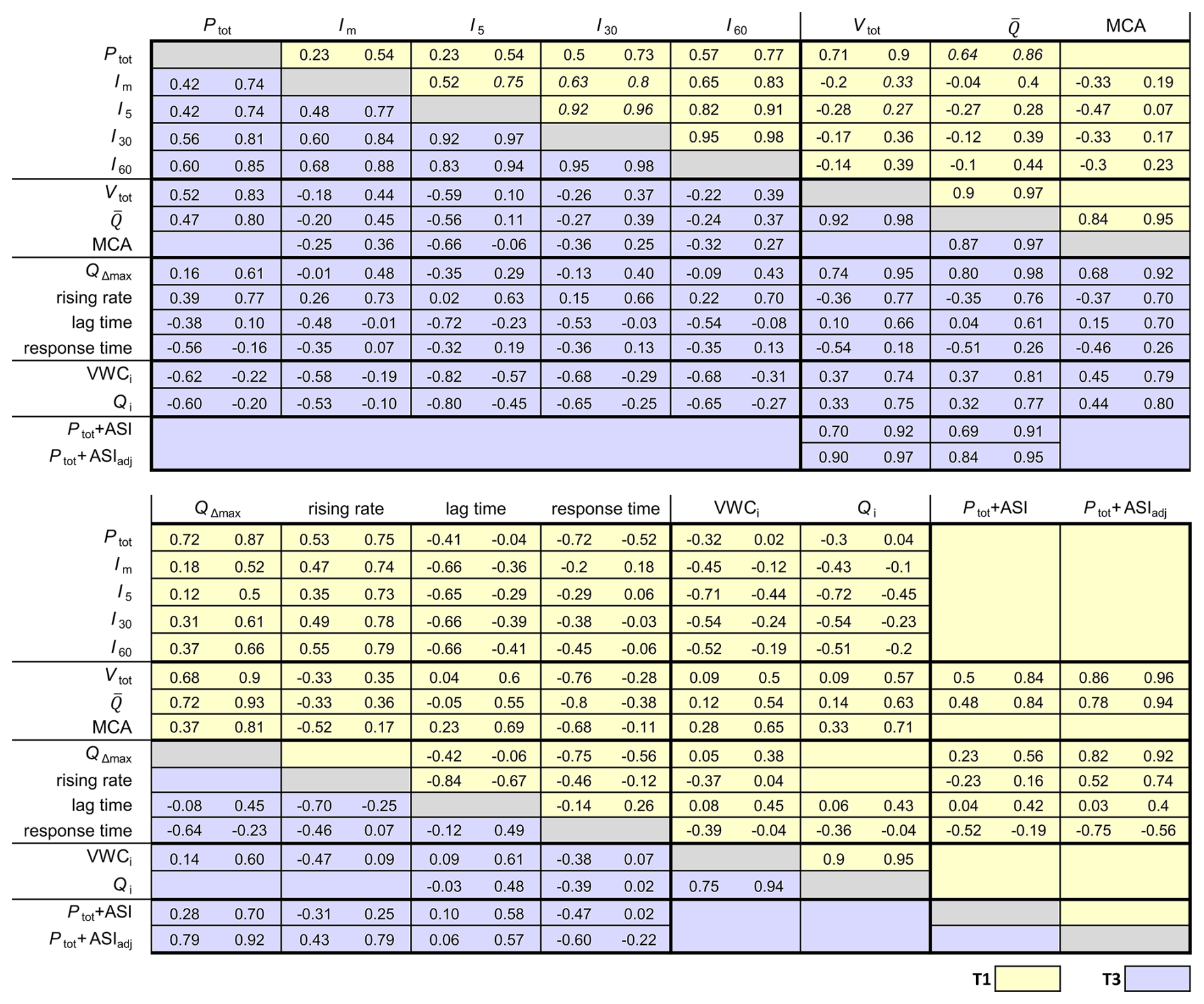
Figure D1 Lower and upper 95 % confidence intervals of the Spearman rank correlations presented in Fig. 8. The confidence intervals were computed using a bootstrap approach (1000 resamples, percentile method; see Sect. 2.3.7).

Appendix E

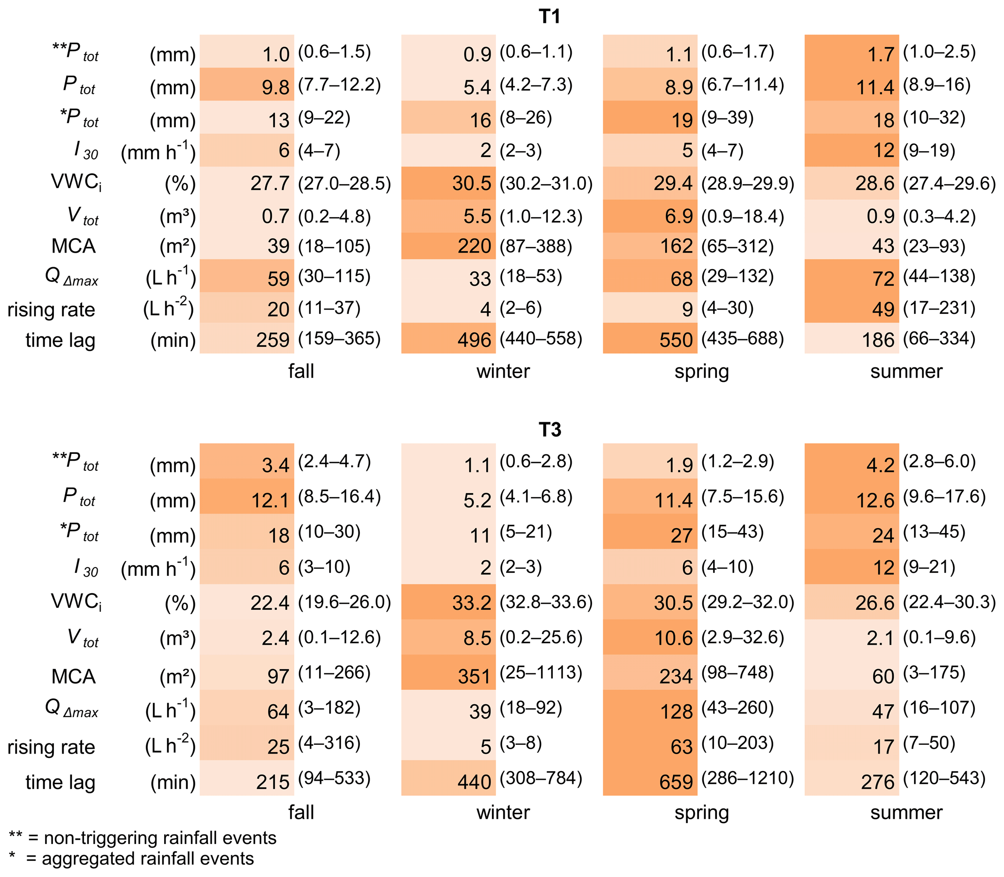
Figure E1 Lower and upper 95 % confidence intervals of the seasonal trimmed means presented in Fig. 19. The confidence intervals were computed using a bootstrap approach (1000 resamples, percentile method).