Critical assessment of metrics and methods used to quantify temporal loading of rainfall events

The distribution of rainfall intensity through time at a fixed spatial location, referred to here as event temporal loading, can significantly influence hydrological and geomorphological responses, including run-off generation, urban flood risk, and soil erosion. Numerous approaches have been developed to analyse rainfall event temporal loading, but these differ in how they characterise rainfall behaviour and in the aspects of storm structure they emphasise. Emerging research further suggests that climate change may alter rainfall temporal loading in complex and regionally dependent ways, underlining the importance of clear and consistent approaches to its quantification. In this study, we identify 48 metrics which have been previously applied to describe event temporal loading, and define a further five metrics representing aspects not fully captured in existing metrics. We calculate these metrics for 233 128 rainfall events recorded at Danish rain gauges. We use data-driven cluster analysis to reveal how the metrics relate, highlighting groups of metrics that describe similar properties, and others that are more distinct. Based on this, we conceptualise five aspects of temporal loading: mass timing, peak timing, magnitude concentration, temporal concentration, and intermittency. We demonstrate that some metrics are robust to changes in rainfall event temporal resolution and pre-processing, while others are highly sensitive. Drawing on these findings, we recommend one representative metric per aspect: the 4th quartile mass fraction (or D₅₀ if a continuous measure is preferred) for mass timing; peak position ratio for peak timing; the Gini coefficient for magnitude concentration; temporal standard deviation for temporal concentration; and the wet-dry transition rate for intermittency. Together, these recommendations provide a practical framework for deliberate metric selection and more consistent cross-study comparison of rainfall temporal loading.

1 Introduction

Rainfall events vary not only in total volume and duration but also in how intensities fluctuate as storms develop. Storms typically progress through phases of initiation, intensification, and dissipation, reflecting the dynamic interplay of meteorological and cloud processes. These processes give rise to storms with complex space–time structure, so that rainfall evolution differs across both time and location. We use the term “event temporal loading” to describe the internal variability of intensity over the course of a storm at a fixed location. This Eulerian perspective is conceptually straightforward and aligns with the conventional representation of storms in hydrological modelling, such as the design storm approach, where temporal variations are condensed into a single-site record of how rainfall intensity varies over time – a hyetograph. Event temporal loading is described in previous research under various names, including intensity profile (Dunkerley, 2021a), storm profile (Kottegoda and Kassim, 1991), rainfall temporal pattern (Wang, 2020), and intra-event rainfall variability (Todisco, 2014). While it is possible in principle to analyse temporal loading from a moving-storm, or Lagrangian, perspective, systematic methods for doing so have not yet been established.

Rainfall event temporal loading has been shown to influence hydrological and geomorphological responses across a wide range of environmental processes, however the direction and magnitude of its effects often vary between studies. For instance, flood modelling experiments have demonstrated that temporal loading alone can produce flood depth differences of up to 35 % under identical rainfall volumes (Hettiarachchi et al., 2018). In landslide studies, early-peaking storms have been associated with greater infiltration and more severe slope instability (Fan et al., 2020). Soil erosion studies exemplify the diverging outcomes in temporal loading studies. Wang et al. (2016) reported greater soil loss from later-peaking storms, while Aquino et al. (2013) found early-peaking events to be more damaging. Such differences underscore that while temporal loading is clearly influential, its specific impacts depend on system characteristics, dominant processes, and methodological approaches.

Extreme rainfall events are expected to intensify in a warming climate at around 6 %–7 % per degree Celsius, following the Clausius–Clapeyron (CC) relationship (Trenberth et al., 2003). Furthermore, for short-duration convective extremes, some studies suggest even greater rates of intensification, known as super-CC scaling (Fowler et al., 2021). This behaviour has been linked to dynamical storm changes under higher temperatures, including variations in storm speed, convective cell development, and feedbacks such as latent heat release (Haerter and Berg, 2009; Fowler et al., 2021). These dynamical storm processes have also been suggested to affect the temporal distribution of rainfall within storms. A growing body of work has begun to examine how event temporal loading may change in a warmer climate (Visser et al., 2023; Ghanghas et al., 2024; Asher et al., 2025a; Wasko and Sharma, 2015), but results to date show variable magnitudes and directions of change, pointing to possible regional dependencies in behaviour. Research in this area remains at an early stage and is developing actively.

Despite its demonstrated importance, rainfall event temporal loading is often simplified in impact modelling applications, particularly in design-oriented or regulatory contexts. This simplification is most commonly achieved using design storms, which are synthetic profiles used to standardise the representation of extreme events across specified return periods, and a longstanding component of engineering practice (Watt and Marsalek, 2013). Design storms combine an estimate of total rainfall with a prescribed hyetograph, which dictates how rainfall is distributed over the course of the storm. While total rainfall depths are typically derived from locally specific statistics, the same hyetograph shape is often applied universally. For example, symmetrical, centrally peaked intensity profiles are commonly used, such as the FEH design profiles in the UK (Centre for Ecology & Hydrology, 1999) and the Chicago design storm in the US and other countries (Keifer and Chu, 1957).

An alternative approach in impact modelling is continuous simulation, in which long-term rainfall time series are routed through models to generate extended sequences of runoff responses that are subsequently analysed to estimate flood magnitudes for given return periods (Boughton and Droop, 2003). This approach inherently accounts for antecedent wetness conditions and avoids many ad hoc assumptions about initial losses, but requires extensive data and substantially greater computational effort. Considerable research has examined the temporal and spatial resolution needed to capture storm dynamics relevant to urban hydrology, with several studies suggesting that sub-hourly (often 1–5 min) data are required to resolve the short, intense bursts that drive urban response (Einfalt et al., 2004; Schilling, 1991). Radar products and stochastic rainfall generators have therefore been developed to provide such high-resolution inputs. Nonetheless, continuous simulation remains less commonly used in routine flood risk assessment and infrastructure design than event-based methods, which continue to be favoured for their simplicity, interpretability, and established role in practice (Boughton and Droop, 2003; Pathiraja et al., 2012; Formetta et al., 2018; Krvavica and Rubinić, 2020).

Robust, interpretable metrics are therefore essential to bridge the gap between observed rainfall behaviour and the simplified forms commonly used in models. By quantifying key aspects of temporal loading, such metrics help preserve important features when rainfall events are simplified, improving the fidelity of hydrological representations. Furthermore, metrics can offer insight into why the influence of temporal loading varies across studies and contexts, by revealing which specific aspects of storm evolution are most relevant to particular hydrological responses. Flood response, for instance, may be especially sensitive to peak intensity and its timing, whereas soil erosion and landslide initiation may respond more strongly to rainfall concentration or intermittency. Despite this, a wide variety of metrics have been proposed with little systematic evaluation of how they relate to one another, how sensitive they are to temporal resolution and data processing choices, or whether they are broadly suitable across different contexts. Terminology is also inconsistent, with metrics often targeting different characteristics, such as asymmetry, peakiness, or intermittency, but these distinctions are rarely made explicit. Applying metrics without regard to these differences risks misplaced emphasis or misinterpretation.

This study seeks to address gaps in knowledge on how temporal loading metrics perform under different data and processing conditions, and on how metrics relate to one another. The work addresses the following research questions:

• RQ1: What key properties of rainfall event temporal loading are commonly measured, and why?

• RQ2: Which metrics are strongly correlated, suggesting they may be redundant or are suitable for use in cross-comparison of studies?

• RQ3: How sensitive are these metrics to the temporal resolution of the rainfall data?

• RQ4: How does conversion of rainfall events to Dimensionless Mass Curves (DMCs) affect metric values?

The first research question is addressed through a structured literature review that identifies existing metrics used to quantify temporal loading, followed by a synthesis of their underlying assumptions, intended applications, and data requirements (Sect. 2). The remaining questions apply data from Danish rain gauges. The second question is tackled using cluster analysis to explore similarities among metrics calculated from raw rainfall events at a 5 min resolution (Sect. 4.1). The third and fourth questions are examined via comparative analyses of metrics calculated on rainfall events at varying temporal resolutions (Sect. 4.2) and after calculation of DMCs (Sect. 4.3). Through this empirical analysis, the study builds toward a practical framework for metric selection, identifying five distinct aspects of rainfall temporal loading and proposing a representative metric for each, with the aim of reducing inconsistency and improving comparability across future studies.

2 Literature review

The literature review is conducted according to the PRISMA (Preferred Reporting Items for Systematic Reviews and Meta-Analyses) framework. This is a standardised method of performing literature review which aims to minimise potential researcher bias. Further methodological details are provided in Supplement Sect. S1. The main outcomes of the literature review are reported in the sections that follow.

2.1 Domains and purposes of reviewed literature

Research into rainfall temporal loading is conducted across domains where hydrological and geomorphological responses to rainfall are important, including flood and hydrological research, pollution modelling, and soil erosion and landslide studies. Across these contexts, research is generally motivated by similar questions. One common aim is to assess system sensitivity to rainfall temporal loading. Running models using rainfall events with fixed total volume and duration but varying temporal distribution allows for impacts to be examined. Research of this nature has been performed in regards to: runoff generation in urban catchments (Cai et al., 2024; Asher et al., 2025b), the hydraulic performance of urban sewer systems (Li et al., 2021), modelling of soil erosion and sediment transport (Römkens et al., 2002; Liu et al., 2022; Dunkerley, 2021a; Rivera et al., 2012; Gao et al., 2024; Wang et al., 2016; Alavinia et al., 2019; Gholami et al., 2021; Aquino et al., 2013; Klamkowski et al., 2012), pollution wash-off (Fu et al., 2021), and rainfall-induced landslides (Fan et al., 2020).

A second common aim is to characterise the temporal loading of rainfall events. This includes research developing new or more nuanced metrics for describing internal rainfall variability (Todisco, 2014; Dunkerley, 2022), or research applying existing metrics in order to group and summarise events into representative hyetographs for specific locations (Wang, 2020; Amin et al., 2000; Dolšak et al., 2016; Vantas et al., 2019). This allows assessment of how well standard hyetographs reflect observed temporal patterns, and the improvement of design storms. A third aim of research on temporal loading is to improve representation of the statistical characteristics of rainfall in stochastic rainfall generation and disaggregation (Wu et al., 2006; Nguyen and Chen, 2022). A final aim is to assess the impact of climate change on extreme rainfall characteristics (Visser et al., 2023; Hu et al., 2018; Asher et al., 2025a).

2.2 Rainfall data sources

The reviewed studies rely on two main sources of rainfall data: observational records and synthetically generated events. The majority of studies use events extracted from observed rainfall time series, typically recorded by rain gauges (e.g., Zhang et al., 2023), or radar (e.g., Urgilés et al., 2024). Events are extracted from observational records at point locations based on assumptions about what constitutes the start and end of a rainfall event, such as minimum intensity thresholds or inter-event dry periods (Restrepo-Posada and Eagleson, 1982). Additionally, event boundaries and characteristics are inevitably shaped by the temporal resolution of the observational dataset, and so “observed” rainfall events remain approximations shaped by the resolution of the measurement system, rather than exact representations of storm behaviour.

Other studies use synthetic rainfall events. Stochastic rainfall generators produce events which reproduce the statistical properties of observed rainfall while allowing control over event magnitude and duration (Cai et al., 2024; Fan et al., 2020). These events are typically used within modelling frameworks to explore a broader range of rainfall scenarios. While this approach enables controlled investigation of temporal effects, it relies on assumptions about what constitutes a “representative” event. This can influence interpretation and limit generalisation to real world rainfall. Idealised design storms are an additional form of synthetic events. These adopt simple geometric profiles, such as uniform rainfall (e.g., the rational method (Smith and Lee, 1984) or triangular hyetographs peaking early, centrally, or late in the event (e.g., Parsons and Stone, 2006). These profiles are used to systematically explore the influence of temporal loading, often forming the basis for physical experiments where pre-defined rainfall patterns are applied to laboratory set-ups simulating hillslopes or infiltration systems (Wang et al., 2023; de Lima et al., 2013; Parsons and Stone, 2006; Zhang et al., 1997). Idealised design storms are pivotal in a lot of the early work on understanding the influence of rainfall temporal loading, however, as temporal structure is prescribed rather than quantified using a metric they are not discussed further here.

2.3 Rainfall processing choices

Rainfall temporal loading metrics may be applied directly to a raw rainfall intensity series, which retains the original units and absolute values of the event, allowing metrics to reflect both timing and intensity. However, metrics are sometimes instead applied to dimensionless mass curves (DMCs). DMCs were originally developed to characterise within-storm temporal structure independently of event magnitude and duration, and have since been widely used in rainfall analysis and design storm construction (Koutsoyiannis and Foufoula-Georgiou, 1993). They are derived by double normalising a rainfall event, scaling cumulative rainfall and event duration between 0 % and 100 %, and expressing the event as a cumulative mass profile. To enable comparison across events with different durations and data resolutions, these dimensionless profiles are typically interpolated at regular fractions of storm duration (e.g. every 1 % or 10 %), producing standardised curves of fixed length (Pan et al., 2017).

The widespread use of DMCs in the literature reflects the need for a standardised representation of rainfall temporal structure that enables direct comparison across events with different durations, magnitudes and numbers of observations. However, the combined effects of double normalisation and interpolation also modify the internal structure of rainfall events, with implications for the behaviour and interpretation of temporal loading metrics. Metrics based on absolute values (e.g. peak intensity) lose their physical units when applied to DMCs, instead reflecting fractions of total rainfall per bin rather than mm h⁻¹. This makes direct numerical comparison with raw equivalents meaningless, though the metrics remain defined and carry information about event shape. Metrics describing timing may become discretised, such that values are constrained to the interpolation intervals (e.g. time of peak occurring at 0 %, 10 %, 20 %, etc. of event duration). As a result, conclusions drawn from metrics applied to raw rainfall and to DMCs may differ.

Table 1 Overview of metrics based on literature review.

Table 2 Overview of metrics defined by authors.

Despite this, studies do not always make explicit whether temporal metrics are calculated using raw rainfall series or DMCs, nor do they consistently discuss the implications of this choice. This lack of clarity complicates comparisons across studies and makes it difficult to determine whether reported differences in temporal structure reflect intrinsic storm behaviour or artefacts of data processing.

2.4 Typology of metrics

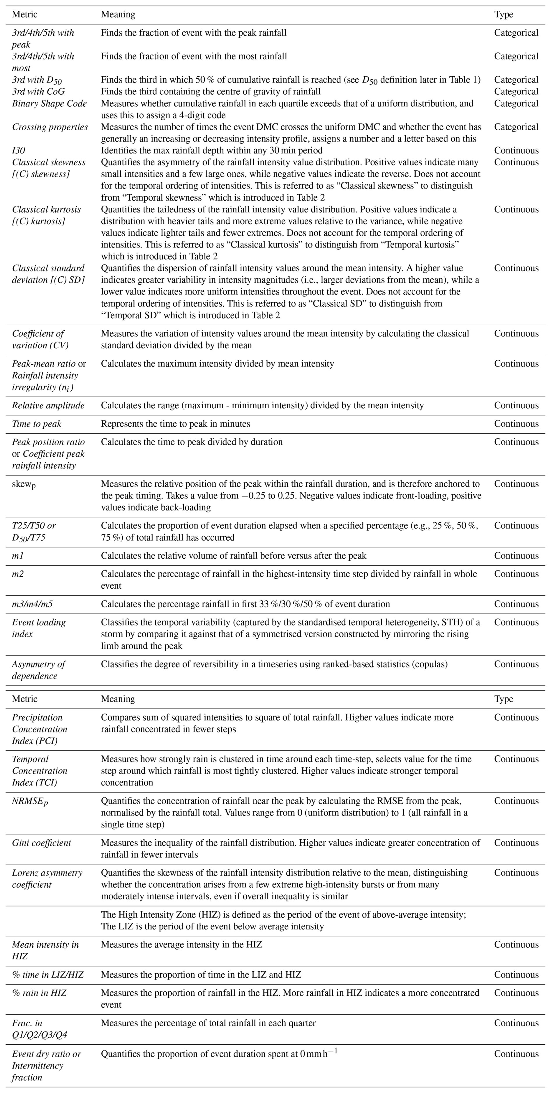
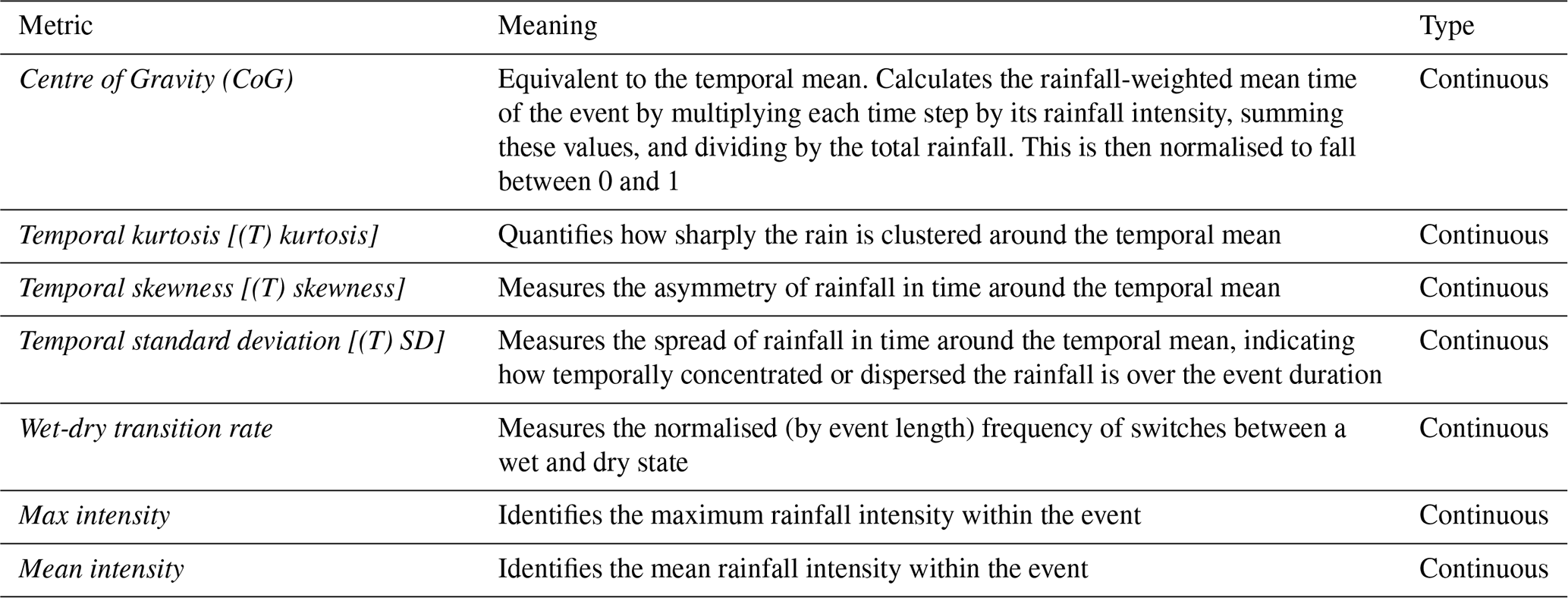
The wide range of metrics identified in the reviewed studies are listed in Table 1. Each metric is categorised as either a categorical or continuous metric. In cases where the same metric formulation is referred to by different names, we list both. In the remainder of the work, we refer to the metric only by the first name listed in Table 1.

2.4.1 Categorical metrics

Those metrics flagged as categorical in Table 1 assign rainfall events to discrete structural classes. Some complex schemes exist, such as the Binary Shape Code (Terranova and Iaquinta, 2011) and Crossing Properties (Kottegoda and Kassim, 1991), both of which compare an event's DMC to a uniform reference profile. Most approaches, however, divide an event into equal fractions (e.g. thirds, quarters or fifths) and identify which fraction contains a defining feature such as the peak intensity or the largest rainfall volume.

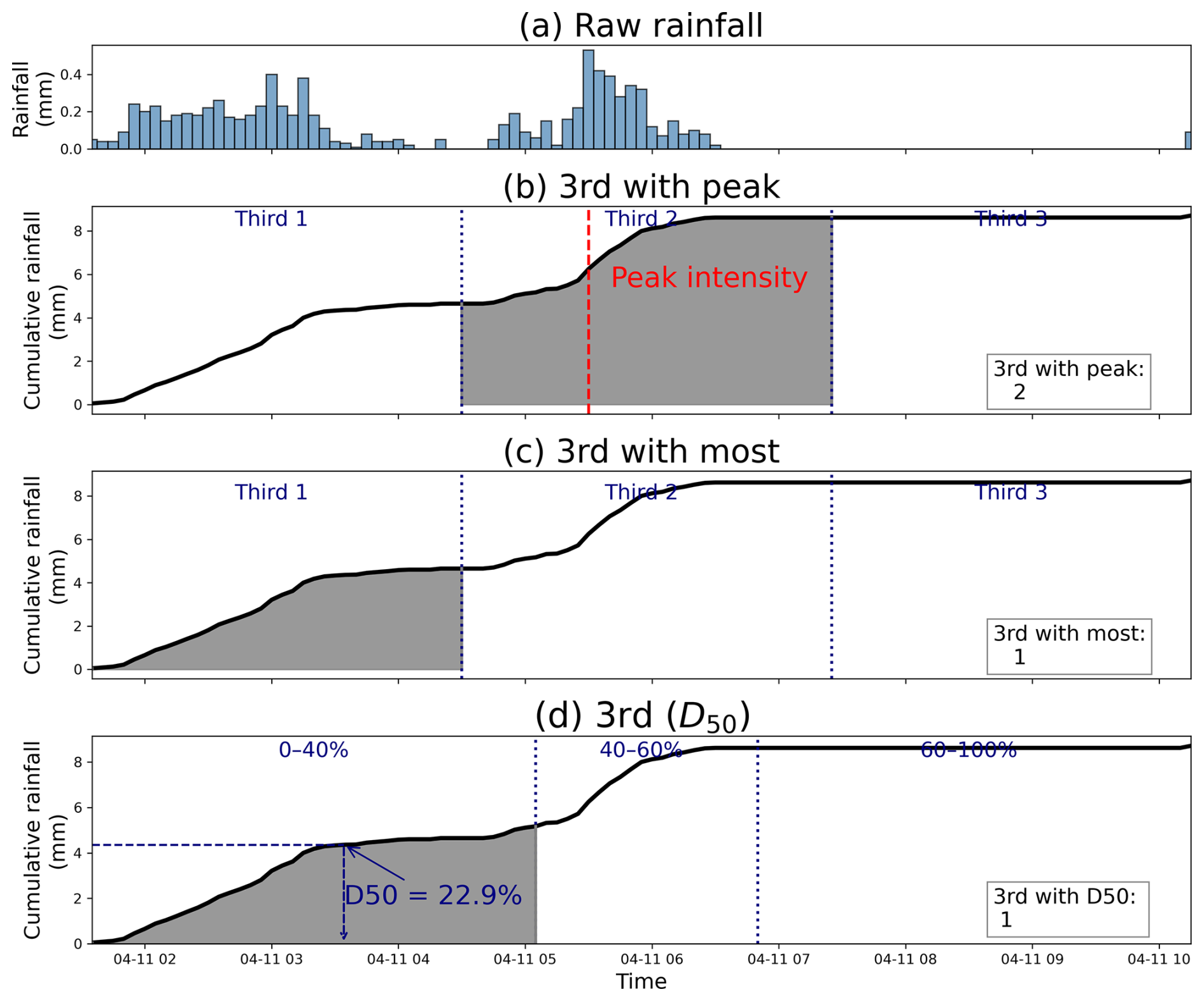
Figure 1 Illustration of some categorical metrics for an example rainfall event: (a) the raw rainfall data, and classification of the event based on (b) 3rd with peak, (c) 3rd with most, (d) 3rd with D₅₀ (NB: these are not even thirds).

While simple, the outcomes of these classification metrics depend heavily on implementation choices. For example, Horner and Jens (1942) introduced the original third-based classification scheme, defining events as advanced, intermediate, or delayed based on the timing of peak intensity. By contrast, Liang et al. (2023) also use thirds but classify events based on the location of rainfall mass, identifying the third with the highest total rainfall. Figure 1 illustrates how these conceptually similar approaches can assign different structural labels to the same event. The 3rd with peak metric classifies the event as centred, since maximum intensity occurs in the middle third, while both 3rd with most and 3rd with D₅₀ identify it as front-loaded, since the majority of cumulative rainfall mass falls within the first third. This has direct implications for the comparability of studies using categorical metrics. A study using 3rd with peak might report that most events are centred, while a study using 3rd with most applied to the same dataset might report that most events are front-loaded. Without careful documentation of which metric was used and what it measures, such differences in reported event structure could be mistaken for genuine differences between study catchments or climates, when in fact they simply reflect differences in metric definition.

Additionally, by reducing a continuous temporal profile to a discrete label, categorical metrics inevitably mask within-class variability. Despite this, they offer a tractable way to group storms by type, reducing complex temporal profiles into interpretable structural classes. This is particularly valuable in design and modelling contexts where consistent, repeatable classification procedures are important.

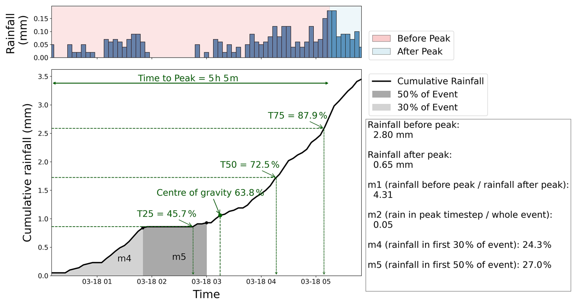
Figure 2 Illustration of several continuous metrics for an example rainfall event, including m1, m2, m4, m5 (Wartalska and Kotowski, 2020), T25, T50, T75 (Knighton and Walter, 2016), centre of gravity and time to peak (Jun et al., 2021; Knighton and Walter, 2016).

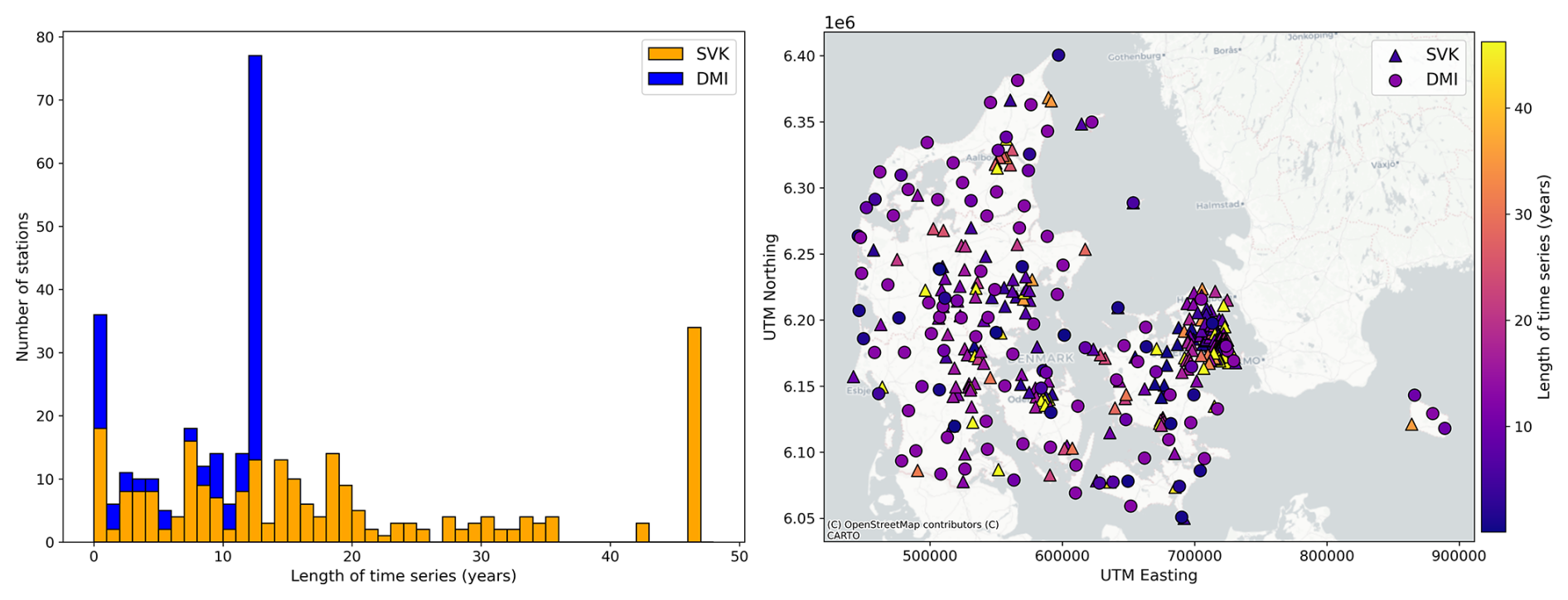
Figure 3 A stacked histogram of the length of the time series for rain gauges (left), and a map of Denmark showing the locations of each gauge, including indications of gauge ownership and time series length (right). Base map: © OpenStreetMap contributors 2025. Distributed under the Open Data Commons Open Database License (ODbL) v1.0.

2.4.2 Continuous metrics

While categorical metrics reduce temporal structure to a discrete label, continuous metrics quantify it using numerical indices. They describe structural properties such as the prominence of intense bursts, the timing of rainfall mass, the degree of concentration into short intervals, and the presence of intermittency. Many continuous metrics aim to quantify similar conceptual properties, such as whether rainfall is early- or late-loaded, but differ in their mathematical construction and therefore in what they actually capture. The distinction between peak-based and mass-based definitions, already seen for the categorical metrics, reappears here. Some metrics define loading in relation to the timing of peak intensity (e.g. peak position ratio), while others use the timing of the bulk of rainfall mass (e.g. D₅₀). In the example event shown in Fig. 2, these perspectives lead to similar interpretations, but this need not always be the case. An event with a short intense burst near the beginning but most of its rainfall occurring later would be classified as early-loaded by a peak-based metric and late-loaded by a mass-based one.

This tension between peak- and mass-based definitions, which run across both categorical and continuous metrics, reflect a broader point: rainfall temporal structure is multidimensional, and no single metric captures it fully. Metric choice therefore shapes interpretation, and different metrics can produce substantively different characterisations of the same event.

2.5 Summary of reviewed studies and metrics

A full overview of the reviewed studies is provided in Table S1 (Supplement Sect. S2). These studies span diverse domains, data sources, processing approaches, and metric types, which reflects the breadth of contexts in which temporal loading is studied. Table S2 (Supplement Sect. S3) summarises the distribution of these characteristics across studies. Despite this diversity, a small number of metrics dominate the literature. As shown in Fig. S1 (Supplement Sect. S3), most metrics appear in only one or two studies. Notable exceptions are the 4th with most metric, which forms the basis of Huff quartiles (Huff, 1967), and the 3rd with peak metric, which underlies the advanced, intermediate, and delayed classification of Horner and Jens (1942). Both have been widely adopted and represent the earliest formal attempts to categorise storm temporal structure. This uneven distribution of metric use, combined with the sensitivity of even the most widely adopted metrics to methodological choices, points to the need for more deliberate and consistent metric selection, which is addressed in the subsequent sections.

3 Methods

3.1 Rainfall data

This research uses rainfall events extracted from Danish rain gauge data at 1 min resolution. Figure 3 shows the national Danish rain gauge network, which is maintained and operated by the Danish Meteorological Institute (DMI). The individual gauges in the network are mainly owned by DMI and the Danish water utilities organised through the “Water Pollution Committee of The Society of Danish Engineers” (abbreviated “SVK” in Danish for “Spildevandskomiteen”). DMI's gauges are weighing rain gauges of the brands Geonor and OTT Pluvio². The measurement resolution of Geonor gauges are 0.1 mm, while the resolution of the Pluvio² gauges started at 0.1 and was updated during the time period focused on in this study to 0.01 mm. SVK's gauges are tipping bucket gauges by Rimco with a measurement resolution of 0.2 mm. Both gauge types record data with a temporal resolution of one minute. Figure 3 (left) shows that all DMI's gauges have been operational for less than 15 years, while there is a much larger spread in time series lengths for the SVK gauges with the oldest ones providing continuous time series from 1979 to the present. Figure 3 (right) shows the spatial locations of the gauges with DMI gauges being relatively evenly spread across the country, while SVK gauges cluster around the major cities.

Data quality control for all gauges in the network are performed manually by DMI's climatology department (DMI, 2025). Data points ruled non-trustworthy by manual quality control are excluded from this study.

3.2 Rainfall event extraction and pre-processing

For each rain gauge, independent rainfall events are extracted over the full period of available data. The rainfall time series is first aggregated to 5 min resolution. This resolution is deemed to best preserve temporal detail, while minimising noise due to the measurement resolution of the rain gauge data. This noise arises because both tipping-bucket gauges and weighing gauges record rainfall in discrete increments, when the buckets tip or when the accumulated weight flips a decimal, which leads to many small, artificial peaks in the 1 min time series.

To ensure event independence, we extract events using a minimum inter-event time (MIT) threshold (Restrepo-Posada and Eagleson, 1982; Molina-Sanchis et al., 2016). An “event” thus constitutes any rainfall separated by at least 11 h of rain-free conditions, following practice in several Danish hydrological studies (Gregersen et al., 2013; Thomassen et al., 2023). This approach ensures that each event begins and ends with non-zero rainfall. The choice of MIT has been shown to play an important role in determining both the number and properties of rainfall events identified (Dunkerley, 2008). In this study, event definition is treated as a fixed preprocessing choice rather than a variable of investigation, reflecting a deliberate scoping decision. While the delineation of event boundaries can influence the timing and relative prominence of peak intensity, and hence derived temporal loading metrics, its effects have been examined in several previous studies, e.g. Dunkerley (2008, 2010, 2015); Wang et al. (2019); Freitas et al. (2020); Molina-Sanchis et al. (2016); Haile et al. (2011); Medina-Cobo et al. (2016); Meier et al. (2016). In contrast, this study focuses on methodological choices that have received less systematic attention, namely the selection and interpretation of temporal loading metrics and their sensitivity to rainfall representation and aggregation.

We define and analyse entire rainfall events, rather than only the most intense “burst” periods, capturing the complete temporal evolution of each storm. Events with less than 4 mm of total rainfall are excluded to remove very light events unlikely to be hydrologically significant. This process produces a dataset of 233 128 rainfall events observed between 1979 and 2025.

Coarser-resolution versions of each event are also derived at 10, 30, and 60 min resolutions. These are generated based on the start and end times of the 5 min event, so for a given coarser resolution, the first timestamp equal to or before the 5 min event start is taken as the new start, and the last timestamp equal to or later than the event end is taken as the new end. As a result, the duration of events at coarser resolutions may be equal or longer than their 5 min counterparts.

3.3 Dimensionless mass curve generation

Dimensionless mass curves (DMCs) are generated from all 5 min resolution rainfall events. A DMC represents the distribution of rainfall within an event, scaled such that both time and accumulated rainfall range from 0 % to 100 %. Each DMC is interpolated to have 10 equally spaced time points. Importantly, while DMCs are typically defined as cumulative profiles, in this analysis we derive a double normalised incremental representation by converting each interpolated DMC back into incremental rainfall. This version reflects rainfall intensity as a proportion of total event mass, distributed over relative time. All temporal loading metrics in this study are applied to these 10-point, double normalised incremental series rather than to cumulative curves. This preserves consistency with how metrics are typically applied to raw rainfall intensities, while enabling direct comparison across events in a dimensionless domain. We additionally apply all metrics to events that have been double normalised but retain their original number of time steps, isolating the effect of normalisation from that of aggregation to 10 points.

3.4 Metric computation and post-processing

Rainfall temporal loading metrics are implemented in Python based on the definitions provided in the original publications. The full codebase for rainfall event extraction and metric calculation is openly available at our GitHub repository (https://github.com/masher92/MetricEvaluation/, last access: 17 June 2026), providing a consistent and reproducible framework for future applications of these metrics. In some cases, the literature lacks sufficient detail on the precise application of metrics (e.g., with respect to temporal resolution, handling of zero values, normalisation procedures). Where ambiguity exists, we make reasonable interpretations of the provided formulations. Two of the metrics identified in Table 1, the Binary Shape Code and the event's Crossing Properties, are not straightforward numeric indicators and are thus deemed outwith the scope of this study.

In addition to the literature-identified metrics, we calculate a set of additional metrics on each event's intensity profile. Firstly, we include the mean and maximum event intensity to aid interpretation of the clustering results. Although these do not describe temporal loading directly, they can help identify cases where other metrics primarily reflect overall magnitude rather than temporal structure. We then calculate several temporal moments, which describe the overall distribution of rainfall intensity through time. These provide a compact and physically interpretable summary of how rainfall mass is positioned, spread, and skewed within an event. Despite their general applicability as distributional descriptors, such metrics have not previously been applied in the context of rainfall temporal structure. Finally, we introduce an author-defined metric, termed the wet-dry transition rate, which quantifies the frequency of wet–dry transitions within an event. This was included to test an event-based representation of intermittency that aligns closely with the intuitive, dictionary definition of the term (i.e., alternation between wet and dry periods). While previous metrics have been proposed to quantify intermittency – for example, the intermittency fraction of Dunkerley (2015), which calculates the proportion of dry time-steps, and the burstiness and memory metrics of Schleiss and Smith (2016) and Dey (2023), which operate on interarrival times over long, multi-event time series – these approaches either measure dry fraction rather than alternation, or require long series to provide stable estimates. The wet-dry transition rate provides a simple, interpretable, event-based alternative that is directly applicable at the scale of individual rainfall events.

3.5 Testing metric overlap and complementarity (RQ2)

To identify metrics which are strongly correlated we apply agglomerative hierarchical clustering based on pairwise metric similarity across all events at 5 min resolution (Jain et al., 1999). Similarity between metrics is quantified using the absolute Spearman rank correlation coefficient, and clustering is performed using average linkage. While clustering directly on metric vectors using Euclidean distance was considered, this would have prioritised numerical proximity over functional similarity. This is problematic because some metrics which have very high negative correlation, and likely describe the same feature, are very distant in Euclidean space. Prior to clustering, each metric is assessed for skewness, and those with an absolute skewness ≤ 1 are retained in their original form. For variables with higher skewness, a logarithmic transformation (log1p) is applied if all values are positive, and otherwise, the Yeo–Johnson transformation (Yeo and Johnson, 2000), which supports zero and negative values, is used. After transformation, all variables are MinMax scaled to common [0,1] range. To inform the number of clusters, we compute silhouette scores for a range of candidate cluster numbers. Silhouette scores quantify how appropriate a cluster number is based on how well each metric fits within its assigned cluster, based upon its similarity to members of its own cluster compared with its dissimilarity to those in other neighbouring clusters (Rousseeuw, 1987). This analysis suggests twelve clusters to be the optimal number (Fig. S2, Supplement Sect. S4).

3.6 Testing sensitivity to temporal aggregation (RQ3)

To assess the sensitivity of each metric to temporal aggregation of rainfall data, we compare metric values computed on rainfall events derived from data aggregated at different temporal resolutions. We treat metrics computed on events from 5 min rainfall data as the reference (“truth”) and compare them to values obtained from coarser aggregations at 10, 30, and 60 min intervals.

For each metric and resolution pair, we quantify both numerical and ranking sensitivity. These two complementary measures allow us to distinguish between metrics which exhibit substantial changes in raw values (numerical sensitivity), those which show shifts in the relative ordering of events (ranking sensitivity), and those which display both or neither aspect of sensitivity.

For continuous metrics, the numerical sensitivity is assessed using the symmetrical median absolute percentage error (sMAPE) (Makridakis and Hibon, 2000). sMAPE measures the absolute percentage error between the metric values at 5 min and at coarser resolutions, and is calculated as:

$$\begin{array}{}\text{(1)}& \text{sMAPE}={\displaystyle \frac{\mathrm{100}}{n}}\sum _{i=\mathrm{1}}^n{\displaystyle \frac{|x_i-y_i|}{\left(\right|x_i|+|y_i\left|\right)/\mathrm{2}}}\end{array}$$

where x_i and y_i are the original and transformed metric values for event i, respectively.

The ranking sensitivity is assessed using Spearman's rank correlation coefficient (ρ), which quantifies the degree to which the relative ordering of events changes due to temporal aggregation, and is calculated as:

$$\begin{array}{}\text{(2)}& \mathit{\rho }=\mathrm{1}-{\displaystyle \frac{\mathrm{6}{\sum }_{i=\mathrm{1}}^n{d}_i^{\mathrm{2}}}{n(n^{\mathrm{2}}-\mathrm{1})}}\end{array}$$

where n is the number of paired observations, $d_i=R\left(x_i\right)-R\left(y_i\right)$ is the difference between the ranks of the ith pair of observations.

For categorical metrics, the % of events in a different category from 5 min at each coarser resolution is used for numerical sensitivity, and Kendall's τ quantifies the ranking sensitivity (Kendall, 1938) by measuring the association between two ranked variables. It is defined as:

$$\begin{array}{}\text{(3)}& \mathit{\tau }={\displaystyle \frac{P-Q}{\sqrt{(P+Q+T)(P+Q+U)}}}\end{array}$$

where $P/Q$ are the number of concordant/discordant pairs, and T is the number of ties only in x, and U is the number of ties only in y. If a tie occurs in both x and y for the same pair, it is not counted in either T or U.

We also visually explore how each metric responds to aggregation by plotting distributions across resolutions (using histograms for continuous metrics, and bar plots for categorical metrics).

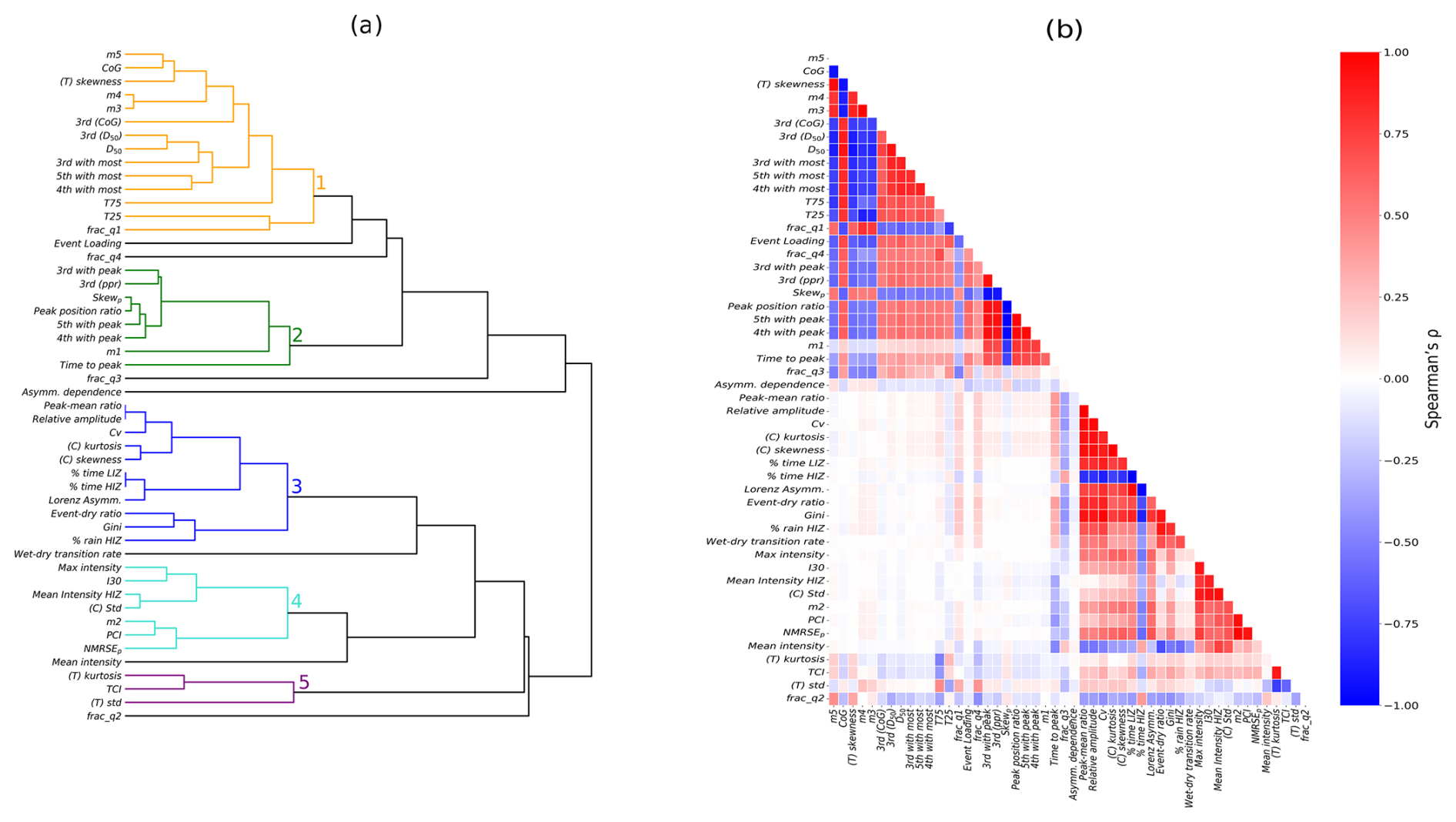
Figure 4 (a) Dendrogram visualising results of hierarchical cluster analysis of the pairwise similarity of metrics across all events. Similarity is quantified using the absolute value of Spearman's ρ, and clustering is performed using agglomerative hierarchical clustering with average linkage and 12 clusters. Clusters with more than one member are highlighted in colour and marked with a cluster number. (b) The full Spearman correlation matrix upon which clustering is based.

We note that comparing continuous and categorical metrics introduces interpretive limitations. When calculating sMAPE scores and plotting metric distributions we opted to not transform or scale metrics. This was to preserve the physical interpretability of each metric, allowing percentage errors to reflect changes in real units (e.g., minutes or intensity proportions) rather than abstracted or standardised values. However, although sMAPE expresses the average percentage difference between two representations (e.g., at different resolutions), the meaning of a given percentage depends on the nature and scale of the metric. For instance, a 70 % sMAPE for a bounded percentile-based timing measure like D₅₀ does not carry the same meaning as a 70 % sMAPE for a scale-dependent metric such as standard deviation. This presents a trade-off, where preserving metric-specific meaning improves interpretability within each metric, but complicates comparative analysis across them. We recognise that we are operating within these constraints, but by interpreting sMAPE scores in conjunction with visual plots, rank correlations, and physical understanding of the metric's behaviour, we can still make valuable assessments of metric behaviour at different resolutions and processing options.

3.7 Testing sensitivity to DMC construction (RQ4)

To evaluate the robustness of rainfall metrics to DMC conversion, we compare values calculated on raw 5 min rainfall events and DMC-transformed rainfall time series. Note that, I30 cannot be calculated, as DMCs have no concept of 30 min. Likewise the Frac. in Q1/2/3/4 can only be calculated on events with n timesteps divisible by 4, and so are not calculated either. Following the methods for temporal aggregation sensitivity testing (Sect. 3.6), we calculate numerical and ranking sensitivity of continuous metrics using sMAPE and Spearman's p, and for categorical metrics using % differences in categorisation and Kendall's τ. Metric value distributions are also compared using histograms for continuous metrics, and bar plots for categorical metrics.

4 Results and discussion: Quantitative metric analysis

4.1 Metric overlap and complementarity (RQ2)

The results of the hierarchical cluster analysis suggest that several well-defined groups of metrics exist. Within each cluster, metrics rank rainfall events similarly. On the dendrogram in Fig. 4a, the shorter the horizontal distance between metrics or groups of metrics, the greater the similarity in rankings. Figure 4b shows the matrix of Spearman's rank correlation scores upon which the clustering is based. Negative correlations arise where metrics respond to the same underlying asymmetry but with reversed directionality – for instance, a front-loaded event will have a lower D₅₀ (proportion of event elapsed when 50 % of cumulative rainfall has fallen), but a higher m3 (proportion of rainfall in the first third).

The clusters that emerge from this analysis form the empirical basis for defining five distinct aspects of rainfall temporal loading, each capturing a different dimension of storm structure. As described in the following sections, four aspects map closely onto the clusters, while the fifth – intermittency – emerges from a combination of its isolated position in the dendrogram and its prominent treatment in the literature. Two clusters are treated as contributing to a single aspect, magnitude concentration, given their shared conceptual basis.

Cluster 1 is the largest, containing fifteen metrics all describing what we term mass timing – the time at which most rainfall falls during an event. The metrics span both categorical and continuous types, yet exhibit very high Spearman's rank correlation coefficients throughout. This suggests that coarser categorical metrics, such as 3rd with most, rank events similarly to more detailed continuous alternatives such as the centre of gravity, despite their differences in construction.

The second cluster contains eight metrics describing a related but distinct aspect: peak timing, the time at which the peak rainfall intensity occurs. Correlation coefficients are again high despite the mixture of categorical and continuous metrics. While most metrics in this group explicitly quantify the timing of the peak time step, interestingly, the metric m1, representing the ratio of rainfall before versus after the peak, is also placed within this cluster. Although m1 is seemingly focused on the balance of rainfall mass distribution rather than peak timing, its position within this cluster suggests that, in practice, it is strongly influenced by peak placement.

Clusters 3 and 4 both relate to what we term magnitude concentration – the degree to which rainfall is unevenly distributed across timesteps in terms of intensity. Although they form distinct clusters, both describe the contrast between high- and low-intensity periods, and are treated here as related parts of the same underlying aspect.

Cluster 3 emphasises distributional imbalance – how unequally rainfall is shared across timesteps, rather than the size of peaks in absolute terms. Peak–mean ratio, relative amplitude, and the coefficient of variation form a subcluster reflecting mean-based contrasts between intense and weak timesteps. classical skewness and classical kurtosis characterise the shape of the intensity distribution. As negative kurtosis is rare in rainfall events (as this would involve lots of high intensity timesteps, accompanied by few low intensity), classical skewness and classical kurtosis generally co-vary, tending to be high in events where rainfall is concentrated into few timesteps. A further subcluster tightly links the % time in LIZ with its complement, % time in HIZ, reflecting their inverse relationship, with Lorenz asymmetry joining nearby as it also quantifies imbalance in the rainfall distribution between wetter and drier periods. In a separate branch, event dry ratio, Gini coefficient, and % of rainfall in the HIZ cluster together, collectively describing how rainfall volume concentrates into a few timesteps, with events scoring high on one metric tending to do so on the others as well.

Cluster 4 shifts emphasis towards the absolute strength of intense phases. Its first subcluster groups maximum intensity and I30 (the maximum intensity in any 30 min period), both capturing the magnitude of the single wettest short-duration period. The second subcluster links mean intensity in the HIZ (timesteps above the event's mean intensity) with classical standard deviation, both reflecting how rainfall is distributed relative to the event mean. The third subcluster contains m2 (percentage of total rainfall in the highest-intensity timestep), PCI, and NRMSE_p. These metrics explicitly compare rainfall in some timesteps with rainfall in other, directly quantifying how concentrated rainfall is within an event. They also share a potential sensitivity to event length, tending to return higher values when an intense burst is embedded in a short event than when it appears in a longer event with more low-intensity timesteps.

The fifth cluster groups temporal kurtosis, temporal standard deviation, and the TCI, defining a further distinct aspect: temporal concentration. Unlike magnitude-based concentration metrics, these only return high values when high-intensity timesteps are tightly grouped in time. Their very low correlation with metrics in other clusters indicates that this dimension of temporal loading is largely independent from the others. An event can have strongly concentrated intensity without that intensity being temporally clustered, and vice versa. This distinction is particularly relevant for applications such as flash-flood risk and soil erosion modelling, where closely clustered high-intensity periods can greatly amplify impacts compared to if high intensity timesteps were spread across an event.

The remaining seven clusters each contain only a single metric, reflecting a range of different situations. Asymmetry of dependence characterises how rainfall intensities evolve over time, identifying whether events intensify and decay at similar rates – a feature potentially relevant for understanding storm generation and event evolution. The event loading index measures the deviation in temporal variability between an observed event and its time-reversed mirror, capturing structural irregularities not represented by other metrics. Both describe properties that are conceptually interesting and may have value in specific applications, but they do not correspond cleanly to any of the four aspects identified above and are not sufficiently general to warrant inclusion as a core component of the framework. The fractional metrics, fraction of rainfall in Q2, Q3, and Q4, are isolated not because they are uniquely informative, but because individually they offer limited descriptive power, with their information more completely conveyed by mass timing metrics such as D₅₀ or 4th with most. Mean intensity was included as a diagnostic to test whether any other metrics are implicitly driven by overall event magnitude rather than temporal structure; its isolation confirms this is not the case.

The wet-dry transition rate is also isolated in the cluster analysis, but unlike the metrics discussed above, we argue for this metric to form the basis of a fifth aspect of temporal loading: intermittency. Intermittency is frequently discussed in the literature, especially in the context of soil erosion (Dunkerley, 2015, 2023), and dry intervals within events have been shown to influence infiltration capacity, such that more intermittent rainfall can be tolerated at higher intensities during wet intervals (Dunkerley, 2021b; Aryal et al., 2007). However, whether such processes are occurring depends on the actual arrangement of wet and dry periods within an event, not simply on the proportion of dry time. Despite this, intermittency has primarily been measured using the event dry ratio (referred to elsewhere as the intermittency fraction, which captures only the proportion of event time that is dry. This creates a conceptual inconsistency: while the literature emphasises the importance of the frequency and sequencing of wet and dry periods, the metrics used typically reduce this to a single duration-based quantity. Two events can share the same dry-time proportion while differing markedly in how fragmented the rainfall is. An event with a single prolonged dry interval is qualitatively different from one in which the same total dry duration is distributed across many short alternating periods. The clustering results confirm this: the event dry ratio groups with measures of magnitude concentration, reflecting the fact that a high proportion of dry timesteps implies rainfall is compressed into fewer wet periods, irrespective of how those periods are arranged in time. In contrast, the wet-dry transition rate remains isolated, suggesting that intermittency – when defined in terms of wet–dry alternation frequency – represents a genuinely distinct dimension of event structure not captured by commonly used metrics. Together with the four aspects identified through the cluster analysis, intermittency forms the basis of the conceptual framework developed in the remainder of this study.

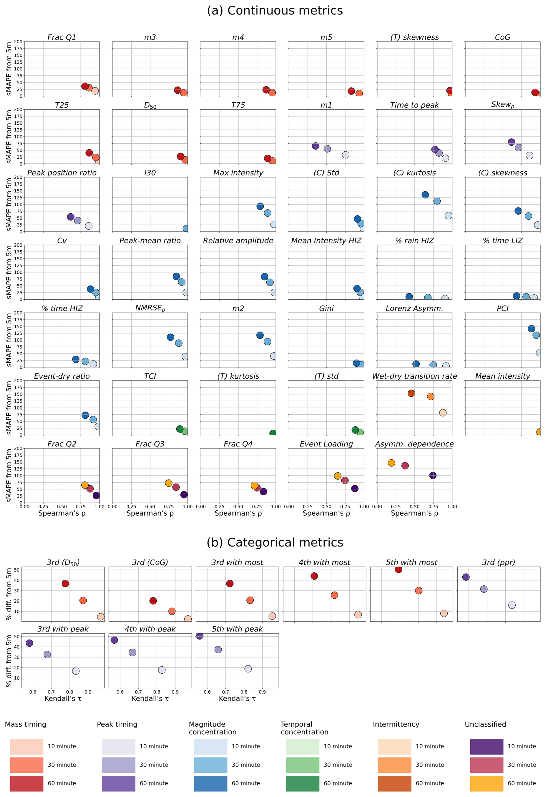
Figure 5 Sensitivity of metrics to temporal aggregation. For each metric (separate subplot), points represent comparisons between the metric calculated at coarser resolutions (10, 30, 60 min) and the reference 5 min data. For (a) continuous metrics, the x-axis shows Spearman's rank correlation coefficient (p) and y-axis symmetrical mean absolute percentage error (sMAPE) relative to the 5 min baseline. For (b) categorical metrics, the x-axis shows Kendall's tau, and y-axis shows the percent disagreement with 5 min baseline.

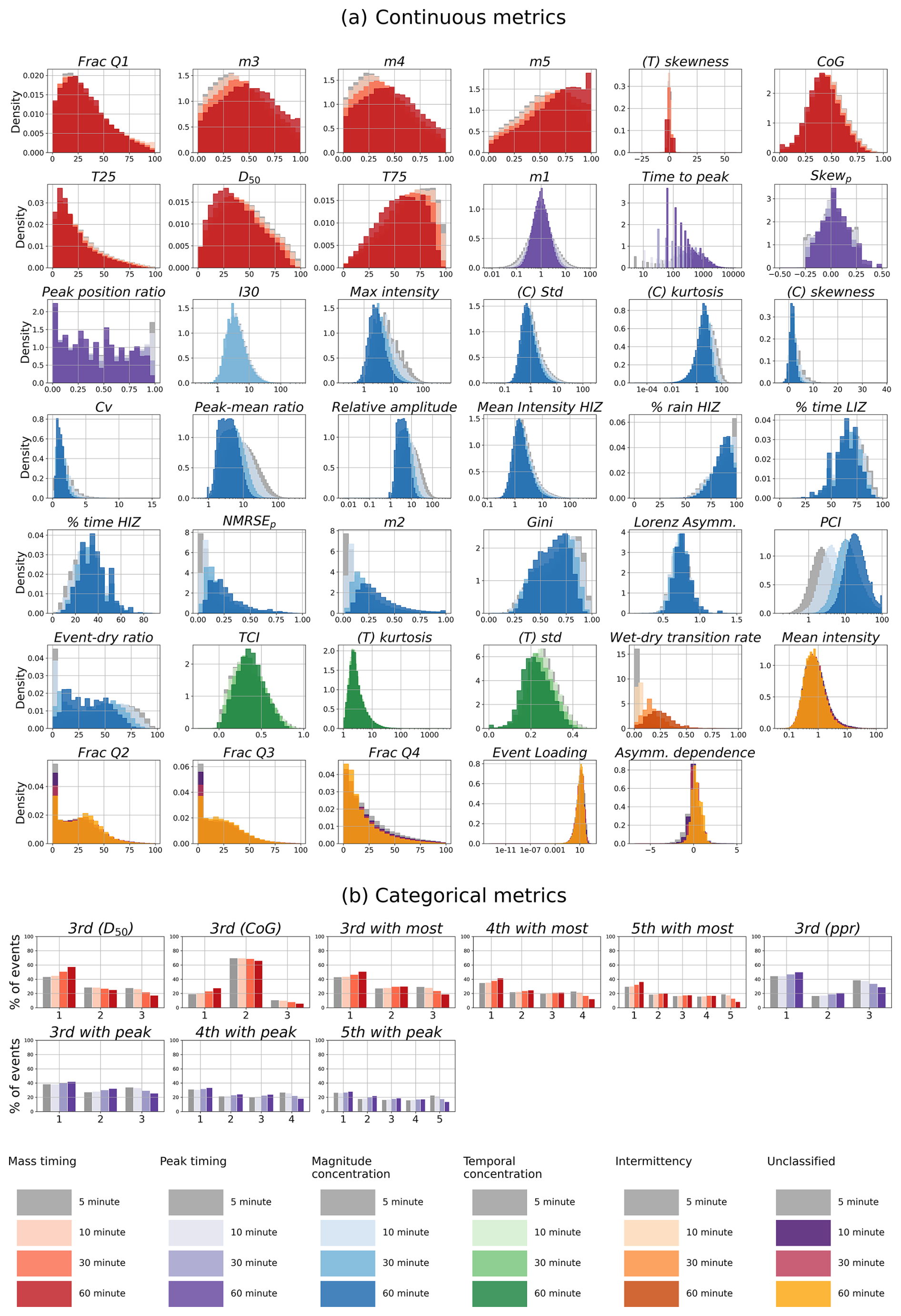
Figure 6 Sensitivity of metric distributions to temporal aggregation. Each subplot shows how the distribution of a given metric changes when calculated on rainfall data at different temporal resolutions (5, 10, 30, 60 min). For (a) continuous metrics, this is shown using overlaid histograms. For (b) categorical metrics, grouped bar charts display the relative frequency of each category across resolutions.

4.2 Sensitivity to temporal aggregation (RQ3)

The sensitivity of each temporal loading metric to changes in rainfall temporal resolution is examined in Fig. 5. Metrics located in the bottom-right corner exhibit high robustness (low numerical and ranking sensitivity), and those trending upwards and to the left show increasing sensitivity to aggregation. Figure 6 complements this by illustrating how full metric distributions shift across temporal resolutions. Results are discussed with reference to the five aspects of temporal loading identified in Sect. 4.1.

Mass timing metrics, including temporal skewness, centre of gravity, and percentile-based measures such as D₅₀ and T75, are among the most robust to temporal aggregation. These metrics summarise the cumulative distribution of rainfall mass rather than individual intensity extremes, and their numerical values and event rankings remain tightly clustered across resolutions. Categorical metrics derived from these quantities, such as 3rd with D₅₀ and 3rd with CoG, are correspondingly stable, though metrics classifying events by the fraction containing the bulk of rainfall show moderate sensitivity – substantially less, however, than those defined by peak timing.

Peak timing metrics show considerably higher sensitivity. Continuous measures describing the position of the peak, such as time to peak and peak position ratio, and those anchored to peak timing including m1 and skew_p, display high numerical and ranking instability under aggregation. Temporal aggregation not only smooths intensities but can displace the apparent timing of the peak, particularly where aggregated values are assigned to the end of time intervals, leading to systematic shifts at coarser resolutions. Distributions for these metrics broaden under aggregation and event rankings are frequently reordered. Categorical metrics based on peak position exhibit a similar pattern. Although this behaviour is conceptually expected, the magnitude and consistency of ranking instability across a large event sample cannot be inferred a priori and therefore warrants explicit quantification.

Within the magnitude concentration group, sensitivity varies depending on metric construction. Metrics explicitly dependent on peak intensity, including peak–mean ratio, relative amplitude, and maximum intensity, show strong numerical sensitivity, with values decreasing at coarser resolutions due to peak smoothing. Conversely, m2, defined as the percentage of rainfall in the peak timestep, increases with aggregation as longer intervals allow the highest-intensity step to capture a larger fraction of total rainfall. In both cases, ranking sensitivity remains comparatively low (Spearman's ρ > 0.8), suggesting that relative event ordering is largely preserved even where absolute values shift. Such metrics may therefore remain useful for comparative analyses across datasets of differing resolution, though absolute values should not be interpreted independently of it. Classical skewness and classical kurtosis show both high numerical and ranking sensitivity, reflecting their mathematical dependence on extreme values directly modified by aggregation. Metrics partitioning events into high- and low-intensity zones (HIZ/LIZ) exhibit more moderate responses, with limited numerical change but some ranking instability. Event dry ratio also shows moderate sensitivity. An event with a high dry ratio is likely to contain at least one substantial contiguous dry period, which would need to be entirely absorbed by coarsening before the metric is meaningfully altered.

Temporal concentration metrics are among the most robust in the analysis. Temporal kurtosis, temporal standard deviation, and the TCI integrate information across the full event duration and are less dependent on the precise magnitude or location of individual peaks. Both numerical values and event rankings remain comparatively stable across resolutions, and distributions in Fig. 6 show only minor shifts, indicating that broader patterns of temporal clustering are largely preserved under aggregation.

The intermittency metric exhibits both numerical and ranking sensitivity to aggregation, and we argue this reflects a fundamental incompatibility between the metric and coarsely aggregated data. At coarser resolutions, intermittent dry periods within events are obscured by aggregation, rendering intermittency effectively unmeasurable. Treating coarse-resolution estimates as meaningful risks drawing incorrect conclusions in applications that depend on accurate characterisation of within-event dry periods, including soil erosion modelling, where dry intervals influence infiltration recovery (Dunkerley, 2019, 2021b), and detection of long-term changes in rainfall intensity. If intermittency increases over time but goes undetected due to coarse temporal aggregation, apparent stability in hourly or daily totals could mask a real increase in wet-period intensity (Schleiss, 2018).

Overall, while some responses to aggregation, particularly for peak-dependent metrics, are intuitive, the results demonstrate that the magnitude and ranking implications are highly metric-specific and cannot always be reliably anticipated without explicit testing. These findings provide a practical reference for metric selection under data constraints. Where only coarse-resolution data are available, mass timing and temporal concentration metrics offer the most reliable characterisation, peak timing and magnitude concentration metrics should be interpreted with caution, and the intermittency metric should be considered unreliable.

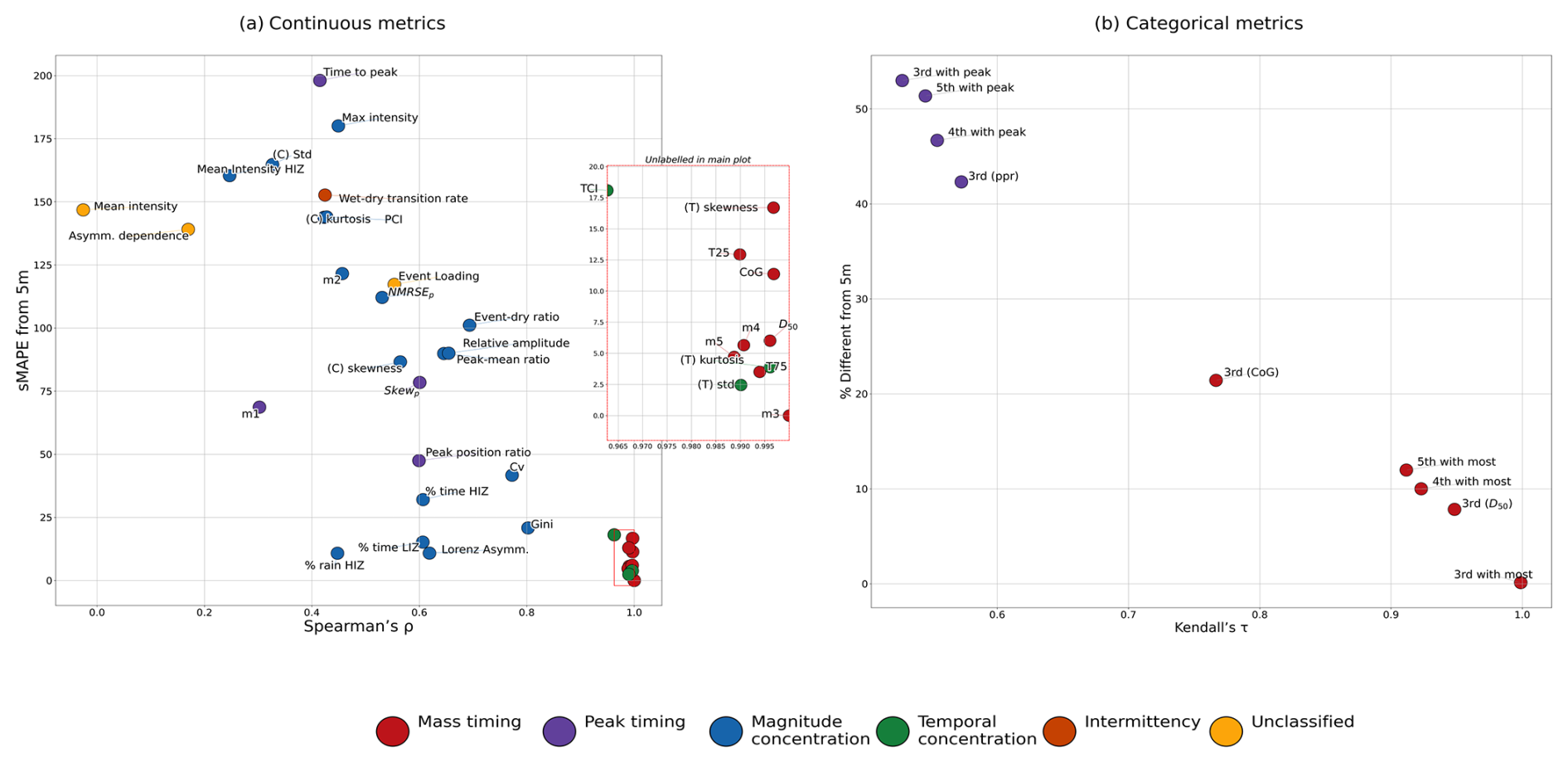
Figure 7 Sensitivity of metrics to dimensionless mass curve representation. For each metric, points represent comparisons between the metric calculated with 5 min raw data and with a 10-point, DMCs calculated on 5 min data. For (a) continuous metrics, the x-axis shows Spearman's rank correlation coefficient (p) and y-axis the symmetrical mean absolute percentage error (sMAPE). For (b) categorical metrics, the x-axis shows Kendall's tau and the y-axis the percent disagreement between the pairs of metric values.

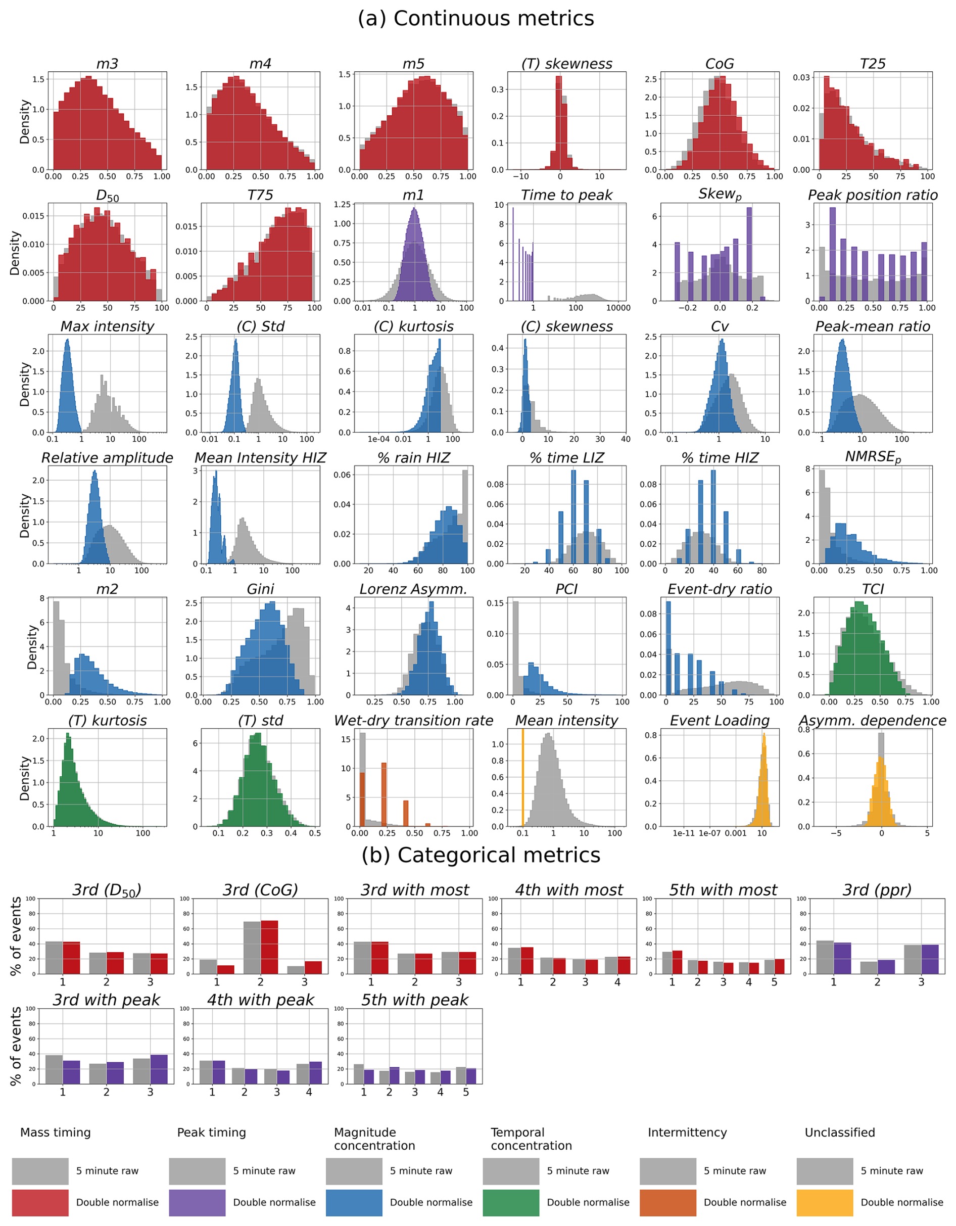
Figure 8 Sensitivity of metric distributions to calculation on DMCs. Each subplot shows how the distribution of a given metric changes when calculated on raw rainfall data at 5 min temporal resolution and on a double-normalised version of the event, interpolated to ten data points. For (a) continuous metrics, distributions are shown using overlaid histograms. Note that gaps in some histograms arise from the discretisation of values when metrics are computed on DMCs–certain metric values are simply not possible, so some histogram bins remain empty. For (b) categorical metrics, grouped bar charts show the relative frequency of each category across resolutions.

4.3 Sensitivity to DMC construction (RQ4)

Sensitivity to conversion of raw 5 min rainfall into double-normalised, 10-step representations (DMCs) varies substantially across temporal loading metrics, as shown in Figs. 7 and 8. Results are discussed with reference to the five aspects of temporal loading identified in Sect. 4.1. The effects of DMC transformation reflect both de-dimensionalisation, with both time and intensity rescaled to a [0,1] domain, and also resolution coarsening through interpolation. Supplement Sect. S5 presents supplementary sensitivity analysis using double-normalised events that retain their original temporal resolution (i.e., without interpolation to 10 time steps).

Mass timing metrics are among the most robust to DMC conversion. Percentile timing measures (T25, D50, T75), moment-based metrics (centre of gravity, temporal skewness), and mass distribution indicators (m3, m4, m5) all show limited numerical and ranking sensitivity, with value distributions remaining largely unchanged after conversion (Fig. 8). These metrics reflect the shape and balance of the event over its duration rather than relying on specific peaks or absolute magnitudes, and are either unitless by construction or meaningful when expressed as proportions of total event time or mass. Categorical metrics derived from these quantities, including 3rd with D₅₀, 3rd with CoG, and those recording the fraction with most rainfall (3rd /4th/5th with most), show corresponding stability.

Peak timing metrics show considerably higher sensitivity to DMC conversion. Metrics such as peak position ratio, skew_p, and m1 are affected both by the interpolation-induced smoothing of sharp transitions and by discretisation arising from the 10-step representation, which constrains values to multiples of 10 % and limits meaningful variation across events. The stepped histograms visible in Fig. 8a illustrate this clearly. As with temporal aggregation, peak displacement under interpolation can reorder event rankings, and this sensitivity is particularly pronounced for metrics anchored to the precise timing of peak intensity.

The effects of DMC conversion on magnitude concentration metrics are more varied. Metrics relying on relative contrasts between timesteps, such as peak–mean ratio, relative amplitude and m2, are affected by interpolation-induced smoothing in a manner similar to temporal aggregation. However, de-dimensionalisation introduces additional consequences not present under aggregation alone. Metrics that depend on absolute intensity contrasts, such as classical standard deviation and coefficient of variation, lose interpretability when all intensities are normalised to a [0,1] domain, as relative differences are compressed and the metric no longer reflects the original signal. Mean intensity becomes entirely uninformative, returning a fixed value of 0.1 in all cases (Fig. 8a). Metrics describing distributional imbalance in relative terms, such as the Gini coefficient, are more stable, as their construction is less dependent on physical units.

Temporal concentration metrics show moderate sensitivity to DMC conversion. The interpolation process smooths sharp transitions between timesteps, which can reduce the apparent clustering of high-intensity periods and affect metrics such as temporal kurtosis and temporal standard deviation. However, because these metrics integrate information across the full event rather than depending on individual peaks, they remain more stable than peak timing metrics, and broader patterns of temporal clustering are largely preserved.

The conclusions drawn above for the aggregation sensitivity of the intermittency metric apply equally to the DMC representation. Interpolation to ten time steps inevitably obscures within-event dry periods, and intermittency derived from DMC events should be treated with the same caution as coarse-resolution estimates. As with aggregation, treating DMC-based intermittency estimates as meaningful risks masking real variability in wet-dry switching behaviour, and we recommend that intermittency is excluded from any analysis based solely on DMC representations.

Overall, these findings reinforce the practical guidance offered by the temporal aggregation analysis. Mass timing and temporal concentration metrics are the most transferable across input representations, while peak timing and magnitude concentration metrics require particular caution when applied to DMC data, and intermittency metrics become meaningless. This distinction is especially relevant when DMCs are used to classify rainfall types or inform design storms, where metric interpretability in the dimensionless domain should be an explicit consideration in metric selection.

Table 3 Five recommended components of rainfall event temporal loading. Each component is described, the associated metrics listed, and a recommended metric identified. Listed metrics robust to temporal aggregation and DMC processing are bolded.

4.4 Recommendations

Based on the findings of the literature review and the data-driven clustering exercise, we recommend breaking event temporal loading into five components: (1) mass timing, (2) peak timing, (3) magnitude concentration, (4) temporal concentration, and (5) intermittency. Table 3 summarises each component, lists the metrics associated with it, and identifies a recommended metric for practical use. The recommended metrics are: the 4th with most rainfall and D₅₀ (mass timing); the peak position ratio (peak timing); Gini coefficient (magnitude concentration); the temporal standard deviation (temporal concentration); and the wet-dry transition rate (intermittency). Recommended metrics are selected on the basis of two criteria. Where a component showed high sensitivity to temporal aggregation or DMC construction, we recommend the metric that proved most robust across resolutions and representations. Where a component showed consistently low sensitivity, we prioritise comparability with existing literature and recommend the simplest and most widely used metric. An exception is mass timing, for which we recommend two metrics – one continuous and one categorical. D₅₀ is recommended as the more precise and informative measure. However, the categorical 4th with most metric is so widely used in the literature and performs sufficiently well in sensitivity testing that we also recommend its continued use, to maintain comparability with existing studies. The equation for each of the suggested metrics are detailed in Eqs. (4), (6)–(9), and (12).

Conceptually, D₅₀ is defined as the percentage of event duration at which 50 % of the total event rainfall volume has accumulated. Given a precipitation rate, r(t), and a precipitation accumulation over time, $P\left(t\right)={\int }_{\mathrm{0}}^{t}r\left(t\right)\mathrm{d}t$, D₅₀ is given by

$$\begin{array}{}\text{(4)}& D_{\mathrm{50}}={\displaystyle \frac{t_{\mathrm{50}}}{t_{\text{end}}}}\end{array}$$

where t_end is the total event duration, and t₅₀ satisfies $P\left(t_{\mathrm{50}}\right)=\frac{\mathrm{1}}{\mathrm{2}}P\left(t_{\text{end}}\right)$.

4th with most is calculated by splitting a rainfall event into four segments of equal duration, and defining this set as $q=\mathrm{1},\mathrm{2},\mathrm{3},\mathrm{4}$. If the total number of time steps is not divisible by four, then the time steps are rescaled accordingly and the precipitation is linearly interpolated to the new time steps. We then define the total sum of precipitation in each quartile as:

$$\begin{array}{}\text{(5)}& P_{\mathrm{q}}=\sum _{i\in T_{\mathrm{q}}}{p}_i,q=\mathrm{1},\mathrm{2},\mathrm{3},\mathrm{4}\end{array}$$

where T_q is the set of time steps in each segment, and p_i is the precipitation accumulation in the ith time step. Finally, 4th with most becomes:

$$\begin{array}{}\text{(6)}& {\text{Q}}_{max}=\underset{q\in \mathit{\{}\mathrm{1},\mathrm{2},\mathrm{3},\mathrm{4}\mathit{\}}}{\text{arg}max}{P}_{\mathrm{q}}\end{array}$$

.

The Gini coefficient is provided by

$$\begin{array}{}\text{(7)}& \text{Gini}={\displaystyle \frac{\mathrm{1}}{\mathrm{2}{n}^{\mathrm{2}}\mathit{\mu }}}\sum _{i=\mathrm{1}}^n\sum _{j=\mathrm{1}}^n\left|p_i-p_j\right|\end{array}$$

where n is the total number of time steps in the event, and μ is the mean precipitation intensity.

The peak position ratio is given as the time step where the peak, t_peak, is located over the total duration of the event, t_end:

$$\begin{array}{}\text{(8)}& \text{PeakPositionRatio}={\displaystyle \frac{t_{\text{peak}}}{t_{\text{end}}}}\end{array}$$

The temporal standard deviation is defined as

$$\begin{array}{}\text{(9)}& {\mathit{\sigma }}_t={\displaystyle \frac{\mathrm{1}}{t_{\text{end}}}}\sqrt{{\displaystyle \frac{{\sum }_{i=\mathrm{1}}^n(t_i-t_{\mathit{\mu }}{)}^{\mathrm{2}}{p}_i}{{\sum }_{i=\mathrm{1}}^n{p}_i}}}\end{array}$$

where t_μ is the centre of gravity and t_i is the time accumulation during the event at time step i:

$$\begin{array}{}\text{(10)}& {\displaystyle }& {\displaystyle }{t}_{\mathit{\mu }}={\displaystyle \frac{{\sum }_{i=\mathrm{1}}^n{t}_i{p}_i}{{\sum }_{i=\mathrm{1}}^n{p}_i}}\text{(11)}& {\displaystyle }& {\displaystyle }{t}_i=(i+\mathrm{1})\mathrm{\Delta }t\end{array}$$

The wet-dry transition rate is the proportion of event duration where a switch between wet and dry states occur:

$$\begin{array}{}\text{(12)}& \text{Wet-dry\hspace{0.17em}\hspace{0.17em}transition\hspace{0.17em}\hspace{0.17em}rate}={\displaystyle \frac{\mathrm{1}}{n}}\sum _{i=\mathrm{1}}^{n-\mathrm{1}}\mathbf{1}(s_i\ne s_{i+\mathrm{1}})\end{array}$$

where 1(⋅) is an indicator function (1 = true, 0 = false), and $s_i=\mathbf{1}(p_i>\mathrm{0})$ is a binary wet/dry indicator.

4.5 Study limitations

It is important to reflect on the representativeness of the rainfall data used in this study. Our analysis draws on the high-quality, dense network of gauges across Denmark, providing over 233 000 well-observed rainfall events. This scale of dataset allows for robust evaluation of metric behaviour under real storm conditions. However, Denmark's temperate maritime climate is not fully representative of the range of rainfall regimes globally. In particular, strongly convective extremes typical of tropical and subtropical climates are less frequent, and storm dynamics may differ from those in arid or mountainous regions. As such, while our findings on the behaviour, sensitivity, and clustering of metrics are expected to generalise across contexts, the specific distribution of rainfall events and the relative prevalence of different temporal loading structures may not. We therefore recommend that future work apply similar analyses in a wider set of climatic settings, both to test the robustness of our methodological conclusions and to build a more globally representative basis for metric selection.

This analysis also has limited ability to assess whether metric choice would materially alter substantive conclusions about rainfall characteristics in a given context. The cluster analysis shows that many metrics rank events in a similar order, but does not consider how those rankings are converted into interpretable outcomes. In practice, this often involves applying thresholds or grouping events–for example, classifying events as front- or back-loaded using D₅₀. Although different metrics may agree on which events are more or less front-loaded, they do not necessarily assign events to the same categories, particularly for events that sit near the classification boundaries. As a result, the same set of events could support different conclusions–for instance, one metric indicating a predominance of front-loaded events, while another suggests a more balanced distribution.

This issue extends to aggregated analyses. Differences in how events are classified can propagate into summary statistics, such as the proportion of front-loaded events or comparisons between catchments and climates. The key limitation is therefore not disagreement in relative ordering, but in how that ordering is translated into categorical or aggregated interpretations. Quantifying the extent to which this influences substantive conclusions was beyond the scope of this study, but represents an important direction for future work.

5 Summary and conclusions

Rainfall event temporal loading, the distribution of rainfall intensity over time at a fixed location, plays an important role in driving hydrological and geomorphological responses such as run-off, urban flooding, and soil erosion. Yet despite its significance, a coherent, consistent approach to its quantification has previously been lacking. This study provides a comprehensive, interdisciplinary review of rainfall event temporal loading metrics, identifying 48 metrics previously applied across scientific domains and introducing five additional metrics to represent aspects not fully covered by existing approaches. Considerable inconsistency in terminology and framing was found across the literature, making it difficult to determine what different studies are measuring, what aspect of storm structure they intend to capture, or whether seemingly similar analyses are directly comparable. The five-component conceptual framework proposed here provides a structured way to distinguish between the key properties of temporal loading and clarify the purpose of different metrics.

All 53 metrics were calculated across 233 128 rainfall events from Danish rain gauge records, and cluster analysis revealed which metrics capture overlapping information and which describe distinct aspects of storm structure. This provided an empirical basis for the suggested five-component conceptual framework and metric recommendations.

Metrics were also evaluated under different data and processing conditions. Sensitivity to temporal resolution was found to vary substantially between metrics: those describing mass timing and temporal concentration are relatively stable under aggregation, whereas metrics related to peak timing and intermittency are highly sensitive. The behaviour of magnitude concentration metrics was more variable, and dependent upon their specific formulation. In addition, transforming events to dimensionless mass curves alters the interpretability of some metrics while leaving others largely unaffected. Given that rainfall data from gauges, radar, and reanalysis products are typically available at differing levels of temporal aggregation, these findings highlight that robustness to data representation is a key consideration. Metric selection should therefore be aligned not only with the aspect of storm structure of interest, but also with the characteristics and limitations of the available data.

Overall, this work provides a clearer understanding of what temporal loading metrics measure, how they relate to one another, and how they behave under different data conditions. It offers a foundation for more explicit, consistent, and reproducible characterisation of rainfall temporal loading, and supports clearer cross-study comparison going forward.