A unified scheme for modeling saturation and infiltration excess runoff

Saturation excess and infiltration excess are two primary surface runoff generation mechanisms governing the timing and magnitude of streamflow at the catchment and larger scales. Despite their frequent co-occurrence and interconnections within catchments, most existing runoff schemes treat these mechanisms separately, following different theoretical paths. This study addresses this theoretical inconsistency by introducing a unified runoff scheme that integrates both mechanisms into a coherent framework. The scheme mathematically expresses both saturation and infiltration excess as functions of the probabilistic distribution of soil water storage, allowing dynamic transitions between mechanisms both in space and time based on the evolving soil water storage distribution during storm events. To demonstrate the applicability of this scheme, we developed a simple hydrologic model and tested it in 181 natural catchments over the U.S., spanning a range of humid to arid climates, and obtained Kling-Gupta efficiencies above 0.5 for 90 % and 70 % of the catchments during the parameter determination and validation periods, respectively. Results show that the model effectively captures the relative dominance of infiltration or saturation excess runoff at the event, seasonal, and annual scales. For instance, model results suggest that infiltration excess runoff dominates where the climate is arid and seasonal evaporative energy and precipitation are in phase, whilst saturation excess runoff dominates under other climate conditions. This unified scheme establishes a new foundation for enhancing the predictive understanding of runoff and other hydrological processes across diverse climates.

1 Introduction

Saturation and infiltration excess runoff are two predominant surface runoff generation mechanisms (Horton, 1933; Dunne, 1978). Infiltration excess runoff, also known as Hortonian overland flow, occurs over unsaturated areas when rainfall intensity exceeds the infiltration capacity of the soil, which remains unsaturated below the surface (Horton, 1933). Saturation excess runoff occurs over saturated areas where the soil is fully saturated at the time of rainfall (Dunne, 1978).

The spatial occurrences of these mechanisms are usually not distributed randomly but rather with complex spatial interplays via soil water movements. These spatial interplays emerge as structured spatial heterogeneity, often referred to as spatial organization (Gaur et al., 2022). For example, there is a spatial organization of saturated areas favoring saturation excess runoff in a catchment, which varies during and between rainfall events, i.e., the variable source area concept (Hursh, 1936; McDonnell, 2003). Furthermore, the spatial distributions of these two mechanisms are often closely interconnected with each other through subsurface water dynamics. For example, saturation excess runoff typically occurs at the lower parts of hillslopes adjacent to streams or lakes where the groundwater table is at the ground surface, while infiltration excess runoff is more common at the upper parts of hillslopes where the groundwater table is below the ground surface (Li et al., 2014; Li and Sivapalan, 2014). The spatial organizations of saturation and infiltration excess occurrences and their interconnections are underpinned directly by the spatial organization of soil moisture (Rodriguez-Iturbe et al., 1995; Western et al., 1999) and indirectly by the spatial organizations of soil (Lin, 2003; Targulian and Krasilnikov, 2007), topography (Rodriguez-Iturbe and Valdes, 1979; Rodriguez-Iturbe and Rinaldo, 2000), and vegetation (Rodriguez-Iturbe et al., 1999; Franklin et al., 2020), with emerging evidence highlighting the role of ecosystem functioning and land–atmosphere interactions in shaping hydrological behavior (Addor et al., 2018; Gao et al., 2023) at the catchment and larger scales.

However, existing runoff schemes for saturation and infiltration excess address these two mechanisms separately, each following distinct theoretical frameworks, despite their common link to soil moisture dynamics. Most infiltration runoff equations, such as the classic Green-Ampt (Green and Ampt, 1911), Horton (Horton, 1933), and Philip (Philip, 1957) equations, are theoretically rooted in Richards' equation for vertical soil water movements and underpinned by the assumptions of spatial homogeneity of relevant landscape properties and time condensation approximation (Sherman, 1943; Sivapalan and Milly, 1989; Smith et al., 2002; Assouline, 2004; Yao et al., 2018). These infiltration equations are essentially point-scale methods, yet they are often applied directly at the catchment scale, oversimplifying the spatial heterogeneities in soil moisture and infiltration capacities within catchments (Sivapalan, 2006; McDonnell, 2007).

Conversely, saturation excess runoff methods explicitly embrace the spatial organization of saturated areas. For example, TOPMODEL uses topographic wetness index distributions to link the spatial distributions of soil saturation and surface topography, assuming the groundwater table is parallel to the land surface (Beven and Kirkby, 1979). Such an assumption is valid only in places where the groundwater table is close to the land surface, e.g., for humid climates, shallow bedrock, and moderate topography (Beven, 1997). Probability distributed models (PDMs) employ a generalized Pareto distribution function to describe the heterogeneity of soil water storage capacity within a catchment. Examples are the HyMOD (Moore, 1985), Xinanjiang (Zhao, 1992), and Variable Infiltration Capacity (VIC) (Wood et al., 1992; Liang et al., 1994) models. In these PDMs, a spatially uniform rise in water storage is assumed within a catchment, except for those locations where the storage capacity is smaller than the precipitation depth during a rainfall event or time step (Yao and Wang, 2022).

The aforementioned theoretical inconsistencies between the existing infiltration and saturation runoff methods, where saturation excess is often analyzed using spatially distributed methods while infiltration excess is typically calculated based on point-scale theories, have led to challenges in achieving a coherent spatial representation of surface runoff processes in hydrologic and land surface models. A typical strategy in large-scale hydrologic models for simulating surface runoff is: (1) Both mechanisms may coexist in a spatial unit, depending on the soil moisture distribution; (2) For saturation excess runoff, a TOPMODEL or PDM-type method is invoked to capture the effects of spatial organization of soil moisture; (3) For infiltration excess runoff, point-scale infiltration methods are implemented, parameterized with the spatial averages of groundwater depth and soil moisture, largely neglecting the effects of spatial organization of soil moisture (Liang et al., 1994; Lawrence et al., 2019). Such a strategy often leads to inaccuracies in surface runoff and flood simulations. For example, previous studies have shown that neglecting sub-grid variability can significantly underestimate runoff generation (Leonarduzzi et al., 2021) and lead to inaccuracies in the timing and frequency of runoff generation (Arora et al., 2001). One exception is that Liang and Xie (2001) used two generalized Pareto distributions in a version of the VIC model to represent the spatial distributions of soil storage and infiltration capacities, respectively. However, in their study, the distribution functions for storage and infiltration capacities are assumed to be independent, rather than dynamically connected.

This study aims to overcome the aforementioned theoretical limitations by proposing a theoretically novel, mathematically unified runoff scheme that coherently represents saturation and infiltration excess runoff and accounts for the transition between the two mechanisms in space and time.

2 Theory

2.1 Theoretical Foundation

Wang (2018) proposed a universal cumulative distribution function (CDF) to describe the spatial distribution of soil water storage capacity at the catchment scale:

$$\begin{array}{}\text{(1)}& F\left(C\right)=\mathrm{1}-{\displaystyle \frac{\mathrm{1}}{a}}+{\displaystyle \frac{C+\left(\mathrm{1}-a\right)S_{\mathrm{b}}}{a\sqrt{{\left(C+S_{\mathrm{b}}\right)}^{\mathrm{2}}-\mathrm{2}a{S}_{\mathrm{b}}C}}}\end{array}$$

Here C is the point-scale soil water storage capacity (in meters) with C≥0. F(C) is the corresponding CDF; a is the dimensionless shape parameter with a range of 0–2; and S_b is the average soil storage capacity (in meters) in a catchment. Introducing the shape parameter allows for flexibility in representing various forms of spatial distributions of soil water storage capacity, ensuring that the CDF can represent a range of catchment types with different topographic organizations and associated soil storage capacity distributions.

Using this new CDF, Wang (2018) provided a theoretical explanation for the Soil Conservation Service Curve Number (SCS-CN) method (SCS, 1972) as a saturation excess runoff model, and revealed the theoretical common ground between the SCS-CN and VIC-type methods. Furthermore, Yao et al. (2020) developed a new PDM by using this CDF to quantify the spatial variability of soil water storage capacity and, hence, saturation excess.

2.2 New Theory

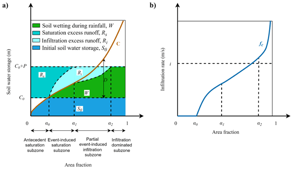
In this study, we propose the Unified Runoff Scheme for Saturation and Infiltration Excess (URSSIE). In URSSIE, we keep the CDF in Eq. 1) for the spatial distribution of soil water storage. A byproduct of Eq. (1) is the spatial distribution of soil moisture deficits (portion of soil storage not occupied by water), which we utilize to derive the spatial distribution of infiltration capacities. This theoretical innovation enables us to incorporate both the spatial distributions of soil water storage and infiltration capacities within a single framework. Figure 1a depicts the spatial distribution of soil water storage capacity (C) with a uniform groundwater depth, similar to the previously discussed PDMs (e.g., HyMOD and VIC). This assumption is reasonable because groundwater table observations are often unavailable, and when the groundwater tables are relatively deep and laterally smooth, spatial differences tend to diminish (Yao and Wang, 2022). Correspondingly, there is a spatial distribution of soil water storage deficit (in meters), D. Usually, the larger the D value, the drier the soil, and the larger the infiltration capacity. Considering a one-to-one relationship between soil infiltration capacity and D, a spatial distribution of infiltration capacity can be yielded as a function of D, as shown in Fig. 1b.

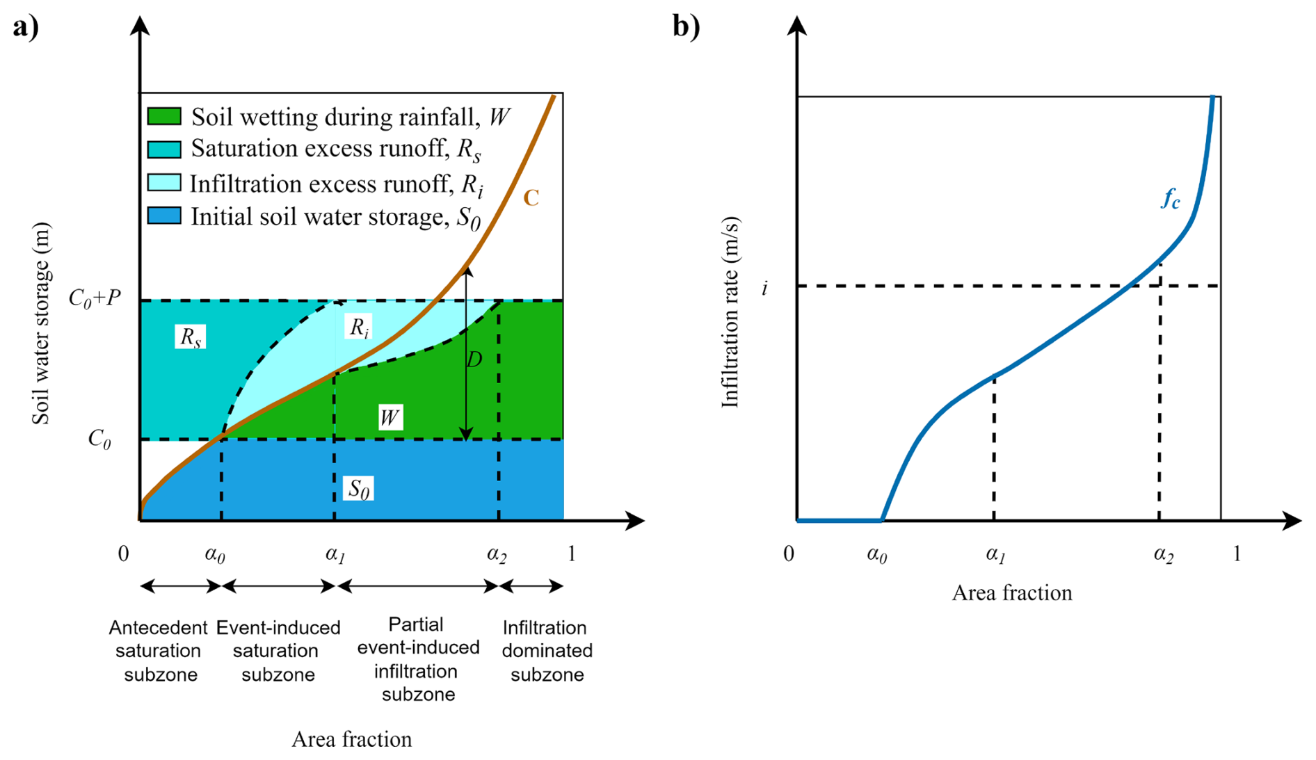
Figure 1 Conceptual framework of URSSIE. (a) Spatial distribution curve of soil water storage capacity. (b) Spatial distribution curve of infiltration capacity. S₀ is initial average soil water storage over the entire catchment; C is soil water storage capacity at a point in space; C₀ is uniform soil water storage across unsaturated zones; P is precipitation depth; R_s is saturation excess runoff; R_i is infiltration excess runoff; D is soil water deficit (C−C₀); W is the soil wetting; i is the rainfall intensity; 0∼α₀, α₀∼α₁, α₁∼α₂, and α₂∼1 are the area fraction ranges of hydrologic subzones that are already saturated at the beginning of the current timestep, will be saturated in current timestep, only having infiltration excess, and having no surface runoff generated, respectively.

We now conceptually divide the whole catchment area into four hydrologic subzones based on their hydrologic responses to rainfall events:

1. Antecedent saturation subzone ($A_{\mathrm{0}\sim {\mathit{\alpha }}_{\mathrm{0}}}$): Infiltration capacity is zero, and all the rainfall becomes saturation excess runoff. α₀ represents the boundaries (–) of where soil is already saturated before the current event or time step.

2. Event-induced saturation subzone ($A_{{\mathit{\alpha }}_{\mathrm{0}}\sim {\mathit{\alpha }}_{\mathrm{1}}}$): This subzone encompasses the areas that will become saturated only during the current rainfall event (or time step). For any point within this subzone, firstly, infiltration excess runoff is generated. Then, the soil becomes fully saturated due to infiltration, and saturation excess runoff generation takes over. α₁ represents the points at which the soil becomes exactly saturated at the end of the current event or time step.

3. Partial event-induced infiltration excess subzone ($A_{{\mathit{\alpha }}_{\mathrm{1}}\sim {\mathit{\alpha }}_{\mathrm{2}}}$): In this subzone, rainfall intensity exceeds the infiltration capacity for either the entire time step or a portion of it, yet the soil remains unsaturated throughout the event. Consequently, only infiltration excess runoff occurs. α₂ represents the points where rainfall intensity is equal to the lowest infiltration capacity during the current event or time step (considering that, at each point, infiltration capacity decreases during the current event or time step).

4. Infiltration-dominated subzone ($A_{{\mathit{\alpha }}_{\mathrm{2}}\sim \mathrm{1}}$): In this portion of the catchment, the infiltration capacity always exceeds rainfall intensity in an event or time step, and no surface runoff is generated.

The boundaries among the four subzones shift during a rainfall event in response to increasing soil water storage and the evolving distribution of infiltration storage capacity across the catchment (see Fig. 2a). α₀, α₁, and α₂ (defined in Eqs. (S27), (S30), and (S32), respectively) may all increase during an event, while not necessarily at the same rate (Fig. 2b). If assuming a rainfall event is sufficiently long, the area fraction for saturation excess runoff generation, α₀, will increase until it approaches 1.0; the area fraction for infiltration excess runoff generation, ${\mathit{\alpha }}^{\ast }-{\mathit{\alpha }}_{\mathrm{0}}$ (α* representing where rainfall intensity equals to infiltration capacity, Eq. S23), will likely decrease in a nonlinear manner until it approaches 0 (Fig. 2c).

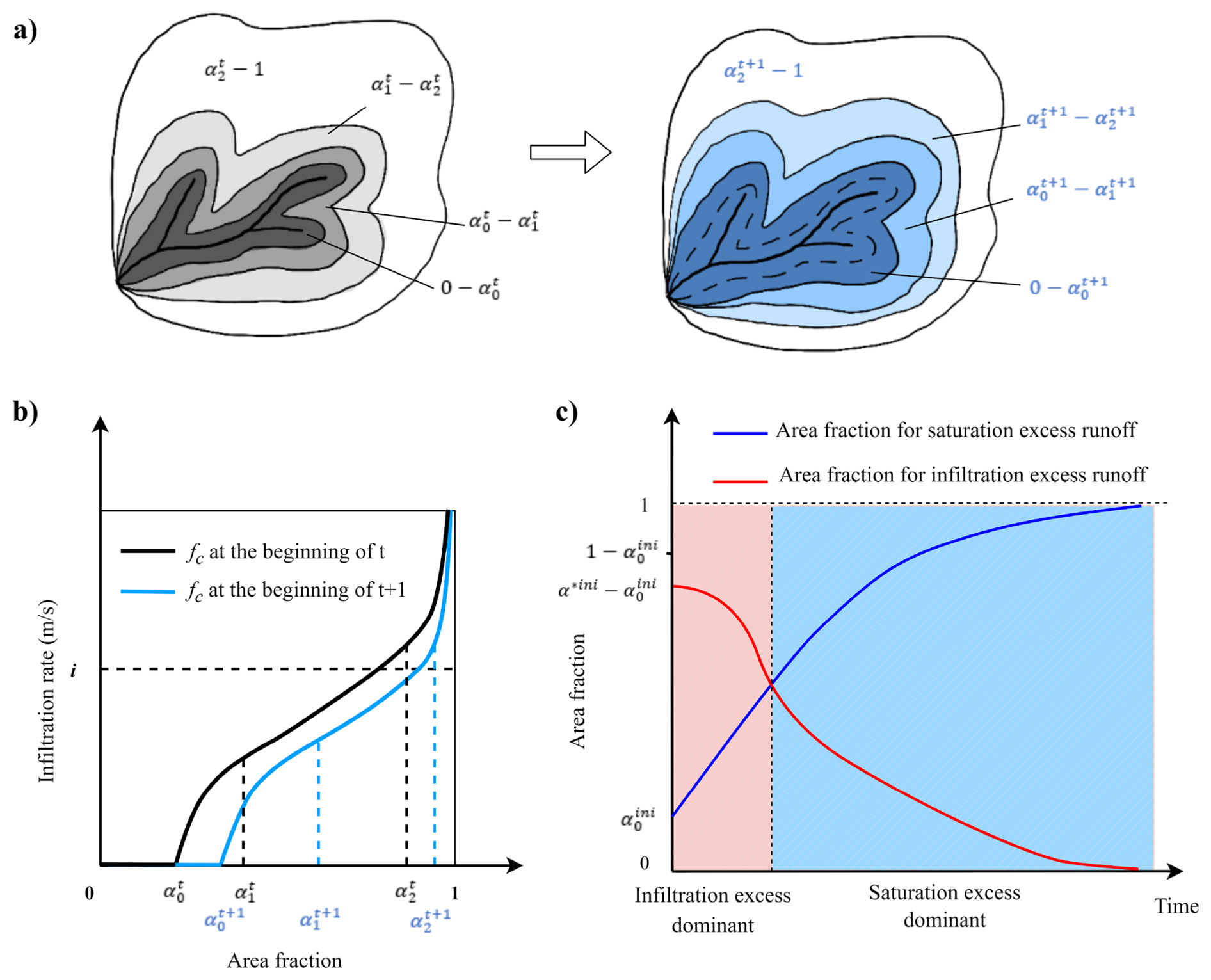
Figure 2 (a) Spatial evolution of infiltration and saturation excess generation areas in two consecutive time steps; (b) Change of infiltration capacity distribution curve in two consecutive time steps; (c) Temporal evolution of subzones for infiltration and saturation excess runoff generation.

Within the URSSIE scheme, the spatial distributions of infiltration and saturation excess generation areas evolve over time (Fig. 2a). The contour lines represent the conceptual boundaries between subzones experiencing different runoff generation mechanisms. The transition zones, depicted by the space between contours from time t to t+1, highlight the dynamic nature of these mechanisms across space within a catchment. At the core of this transformation is the interplay between four distinct subzones: $A_{\mathrm{0}\sim {\mathit{\alpha }}_{\mathrm{0}}}$, $A_{{\mathit{\alpha }}_{\mathrm{0}}\sim {\mathit{\alpha }}_{\mathrm{1}}}$, $A_{{\mathit{\alpha }}_{\mathrm{1}}\sim {\mathit{\alpha }}_{\mathrm{2}}}$, and $A_{{\mathit{\alpha }}_{\mathrm{2}}\sim \mathrm{1}}$. As time progresses from t to t+1, the boundaries between these subzones evolve, reflecting the shifting dominance of saturation-excess and infiltration-excess runoff processes. When more catchment areas become saturated due to antecedent conditions or due to ongoing infiltration, the area contributing to saturation-excess runoff increases. This expansion occurs at the expense of the unsaturated subzones. The transition zones between the contours at time t and t+1 represent areas where infiltration mechanisms undergo significant changes. These zonal changes capture the gradual shift from infiltration-excess to saturation-excess runoff as the catchment becomes wetter (Fig. 2c).

Figure 2b summarizes the dynamic evolution of the subzones in the form of the spatial distribution curves of infiltration capacity at the beginning of time step t and t+1, respectively. The rightward shift of the infiltration capacity curves indicates a progressive decline in the soil's capacity to infiltrate water. In other words, as water infiltrates, the water deficit D decreases, leading to a corresponding decrease in overall infiltration capacity. Figure 2c further illustrates the temporal evolution of the areas for infiltration and saturation excess runoff generation over time, assuming the rainfall duration is sufficiently long. The area for infiltration excess runoff gradually decreases as the groundwater table rises due to increased soil water storage and a decrease in unsaturated areas. On the contrary, the area for saturation excess runoff increases and eventually dominates over the whole catchment area. Overall, the dynamic nature of these subzones and their transitions in Fig. 2 highlights the spatiotemporal variability of runoff generation processes across the landscape owing to the complex interplay between antecedent conditions, rain event characteristics, and the spatial heterogeneity of landscape conditions.

To mathematically express the above conceptual framework, a formula directly linking D and soil infiltration capacity is necessary. There is a close causal relationship between them, i.e., the larger the D value, the drier the soil (particularly the topsoil layers), and thus the higher the infiltration capacity, as suggested by previous experimental and theoretical studies (Liu et al., 2011; Yao et al., 2018; Yang et al., 2020). However, classic infiltration equations do not provide such a linkage to represent the spatial distribution of initial soil moisture (Horton, 1933; Green and Ampt, 1911; Philip, 1957). We represent the point-scale infiltration capacity (f_c) at any unsaturated location in a catchment as a power-law-type function of D:

$$\begin{array}{}\text{(2)}& f_{\mathrm{c}}=m_k{\left({\displaystyle \frac{D}{S_{\mathrm{b}}}}\right)}^n\end{array}$$

Where D is the point-scale soil water deficit (in meters) at a given time. The coefficient, m_k (m s⁻¹), sets the upper limit of infiltration capacity under extreme rainfall conditions. We recommend m_k to be within a range of 0 to $\mathrm{2.315}\times {\mathrm{10}}^{-\mathrm{5}}$ m s⁻¹. The $\mathrm{2.315}\times {\mathrm{10}}^{-\mathrm{5}}$ m s⁻¹ value is slightly above the maximum historical daily rainfall intensity worldwide, 1825 mm d⁻¹ (Holland, 1993). The dimensionless exponent, n, reflects the spatial heterogeneity of landscape conditions within a catchment, such as vegetation cover and soil properties, which can be interpreted as a simplified representation of root-zone and ecosystem controls on infiltration behavior (Savenije, 2024; Gao et al., 2024). It adjusts the non-linearity of the relationship between D and f_c and thus controls the response curve of the infiltration capacity to changes in soil moisture conditions. In this study, we recommend the range of n between 0.4 and 1.0 for the purpose of numerical modeling based on our numerical tests over the natural catchments in the United States (figure not shown). Water deficit ratio, $D/S_{\mathrm{b}}$, indicates the overall soil moisture status: the higher the ratio, the drier the soil, and hence the larger the infiltration capacity. It thus acts as the dynamic scaling factor crucial to modeling how changes in soil moisture adjust the infiltration capacity. As noted by previous studies (Kollet and Maxwell, 2008; Soylu et al., 2011), a shallow groundwater table has a significant impact on surface soil moisture and infiltration capacity. As the groundwater table deepens, its influence diminishes and becomes decoupled from surface soil moisture.

Figure 3 illustrates how the infiltration capacity f_c responds to changes in $D/S_{\mathrm{b}}$, conditioned by varying values of the exponent n with an illustrative value of m_k=500 mm d⁻¹. For low values of n (e.g., n=0.4 or 0.5), the infiltration capacity remains relatively high even at low water deficit ratios. This scenario is typical for clay-rich soils, where the infiltration rate is less sensitive to variations in soil moisture. In such cases, saturation excess may dominate, as the infiltration capacity remains higher than the incoming rainfall intensity. Conversely, for high values of n (e.g., n=0.9), the infiltration capacity increases rapidly with increasing water deficit ratios. This scenario is more representative of sandy or loamy soils, where the infiltration rate is susceptible to changes in soil moisture. In these cases, infiltration excess may dominate, as the infiltration capacity can quickly drop below the rainfall intensity, leading to the generation of surface runoff over unsaturated areas.

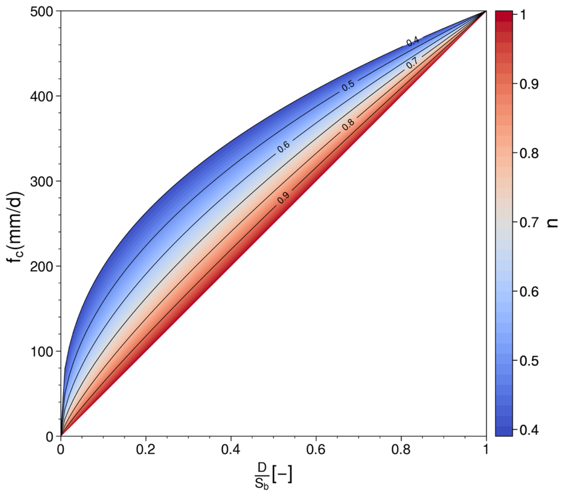
Figure 3 The effects of parameter n values in the basic assumption: $f_{\mathrm{c}}=m_k{\left(\frac{D}{S_{\mathrm{b}}}\right)}^n$ on the relation of infiltration capacity (f_c) and water deficit ratio ($\frac{D}{S_{\mathrm{b}}}$), with m_k set to 500 mm d⁻¹.

Rearranging Eq. (2), we can express D as:

$$\begin{array}{}\text{(3)}& D=f_{\mathrm{c}}^{\frac{\mathrm{1}}{n}}{m}_k^{-\frac{\mathrm{1}}{n}}{S}_{\mathrm{b}}\end{array}$$

D can also be directly calculated as the difference between the point-scale soil storage capacity C (m) and the initial storage C₀ (m):

$$\begin{array}{}\text{(4)}& D=C-C_{\mathrm{0}}\end{array}$$

By combining Eqs. (3) and (4) and solving for C, we obtain:

$$\begin{array}{}\text{(5)}& C=C_{\mathrm{0}}+f_{\mathrm{c}}^{\frac{\mathrm{1}}{n}}{m}_k^{-\frac{\mathrm{1}}{n}}{S}_{\mathrm{b}},\end{array}$$

Eq. (5) allows us to link point-scale infiltration capacity with soil storage capacity and, importantly, dynamic soil moisture conditions. Next, we substitute Eq. (5) into Eq. (1), and yield the probabilistic distribution of infiltration capacity as a function of the dynamic soil water storage changes over unsaturated areas in a catchment:

$$\begin{array}{}\text{(6)}& \begin{array}{rl}& H\left(f_{\mathrm{c}}\right)=\mathrm{1}-{\displaystyle \frac{\mathrm{1}}{a}}+\\ & {\displaystyle \frac{C_{\mathrm{0}}+f_{\mathrm{c}}^{\frac{\mathrm{1}}{n}}{m}_k^{-\frac{\mathrm{1}}{n}}{S}_{\mathrm{b}}+\left(\mathrm{1}-a\right)S_{\mathrm{b}}}{a\sqrt{{\left(C_{\mathrm{0}}+f_{\mathrm{c}}^{\frac{\mathrm{1}}{n}}{m}_k^{-\frac{\mathrm{1}}{n}}{S}_{\mathrm{b}}+S_{\mathrm{b}}\right)}^{\mathrm{2}}-\mathrm{2}a{S}_{\mathrm{b}}\left(C_{\mathrm{0}}+f_{\mathrm{c}}^{\frac{\mathrm{1}}{n}}{m}_k^{-\frac{\mathrm{1}}{n}}{S}_{\mathrm{b}}\right)}}}\end{array}\end{array}$$

Depending on the rainfall intensity i (in m s⁻¹), two cases are evident for the actual infiltration rate f (m s⁻¹) in unsaturated areas. The first case occurs when i≤f_c at time t (in seconds). As such, the actual infiltration rate f=i. In the second case, i>f_c, hence f=f_c. For the second case, the decrease of f with increasing cumulative infiltration F (in meters), can be expressed by:

$$\begin{array}{}\text{(7)}& f=f_{\mathrm{c}}=m_k{\left({\displaystyle \frac{D_{\mathrm{0}}-F}{S_{\mathrm{b}}}}\right)}^n\end{array}$$

Taking the derivative of Eq. (7) (see Supplement for details), we get

$$\begin{array}{}\text{(8)}& {\displaystyle \frac{\mathrm{d}f}{\mathrm{d}t}}=f{\left({\displaystyle \frac{D_{\mathrm{0}}-F}{S_{\mathrm{b}}}}\right)}^{n-\mathrm{1}}\left(-{\displaystyle \frac{m_{k}n}{S_{\mathrm{b}}}}\right)\end{array}$$

Eq. (8) gives how the change rate of f depends on both f itself and F. As F increases, this derivative typically becomes more negative, indicating that the infiltration rate decreases more rapidly over time as the soil approaches saturation. Rearranging and substituting Eq. (7) into Eq. (8) and integrating both sides of the equation from t = 0 to t for dt and from f=f₀ to f for df (see Supplement for details), we obtain a new expression for the infiltration rate as a function of time:

$$\begin{array}{}\text{(9)}& f={\left(m_k^{\frac{\mathrm{1}-n}{n}}{\left({\displaystyle \frac{D_{\mathrm{0}}}{S_{\mathrm{b}}}}\right)}^{\mathrm{1}-n}+{\displaystyle \frac{n-\mathrm{1}}{S_{\mathrm{b}}}}{m}_k^{\frac{\mathrm{1}}{n}}t\right)}^{\frac{n}{\mathrm{1}-n}}\end{array}$$

During a storm event (or a timestep), if the initial infiltration capacity of a spatial point is smaller than the rainfall intensity, infiltration excess begins immediately. The saturation time, t_s1 (in seconds), is the time lapse from the beginning of the timestep to when the soil is saturated. The infiltration rate f at the saturation time is 0. Substituting f=0 and from t=t_s1 into Eq. (9), we obtain the saturation time t_s1 as:

$$\begin{array}{}\text{(10)}& t_{s\mathrm{1}}={\displaystyle \frac{D_{\mathrm{0}}^{\mathrm{1}-n}{S}_{\mathrm{b}}^n}{m_k\left(\mathrm{1}-n\right)}}\end{array}$$

If the initial infiltration capacity is greater than the rainfall intensity i, infiltration excess does not start until the infiltration capacity decreases to i. There thus exists a critical soil water deficit value D_i (in meters) satisfying the condition f_c=i, which can be substituted into Eq. (3) to obtain:

$$\begin{array}{}\text{(11)}& D_i={\left({\displaystyle \frac{i}{m_k}}\right)}^{\frac{\mathrm{1}}{n}}{S}_{\mathrm{b}}\end{array}$$

Correspondingly, there is a critical areal fraction, α^∗, which stands for the locations where D₀=D_i. Ponding time, t_p (in seconds), is the time lapse from the beginning of the timestep to when infiltration excess starts, and can be obtained as $t_{\mathrm{p}}=\frac{D_{\mathrm{0}}-D_i}{i}$. Since the moment of t_p, infiltration continues; after another duration of time, t_si, soil saturation is reached, and saturation excess takes over. t_si can be obtained by using D₀=D_i in Eq. (10).

$$\begin{array}{}\text{(12)}& t_{\mathrm{si}}={\displaystyle \frac{D_i^{\mathrm{1}-n}{S}_{\mathrm{b}}^n}{m_k\left(\mathrm{1}-n\right)}}\end{array}$$

The relationship between t_si and the timestep length, Δt (in seconds), determines the infiltration excess occurrence in different subzones of the catchment. We can consider two distinct conditions based on this relationship.

• i.

  Condition-I, t_si>Δt: In this case, α^∗ falls in α₁∼α₂ and infiltration excess occurs in both the $A_{{\mathit{\alpha }}_{\mathrm{0}}\sim {\mathit{\alpha }}_{\mathrm{1}}}$ and $A_{{\mathit{\alpha }}_{\mathrm{1}}\sim {\mathit{\alpha }}_{\mathrm{2}}}$ subzones. For the $A_{{\mathit{\alpha }}_{\mathrm{0}}\sim {\mathit{\alpha }}_{\mathrm{1}}}$ subzone, infiltration excess occurs in the initial stage of the timestep, and then is taken over by saturation excess. For the $A_{{\mathit{\alpha }}_{\mathrm{1}}\sim {\mathit{\alpha }}_{\mathrm{2}}}$ subzone, infiltration excess starts either at the beginning of the timestep (over some locations within the subzone) or after the ponding time (over the rest of the subzone), but saturation excess does not occur.

• ii.

  Condition-II, t_si<Δt: Here α^∗ falls within the $A_{{\mathit{\alpha }}_{\mathrm{0}}\sim {\mathit{\alpha }}_{\mathrm{1}}}$subzone. For the $A_{{\mathit{\alpha }}_{\mathrm{0}}\sim {\mathit{\alpha }}_{\mathrm{1}}}$ subzone, infiltration excess first occurs either at the beginning of the timestep or after the ponding time, and then is taken over by saturation excess. For the $A_{{\mathit{\alpha }}_{\mathrm{1}}\sim {\mathit{\alpha }}_{\mathrm{2}}}$ subzone, no infiltration excess occurs until after the ponding time, and saturation excess never occurs.

Total surface runoff over a given timestep Δt can be calculated as the sum of infiltration excess and saturation excess runoff generated from all catchment fractions except for the $A_{{\mathit{\alpha }}_{\mathrm{2}}\sim \mathrm{1}}$ subzone.

3 Demonstrative Application

To demonstrate how URSSIE works, we develop a simple hydrologic model based on Yao et al. (2020), primarily by replacing their PDM runoff generation scheme with URSSIE (see Fig. S1 in the Supplement). We then apply this catchment-scale model to over 180 natural catchments across the contiguous U.S. under various climate and landscape conditions. Note that the model presented here is demonstrative and simple, making it unsuitable for comparison with complex, well-established models like TOPMODEL or VIC. In this study, we assume spatial homogeneity of rainfall intensity within small catchments, consistent with classic hydrological models (Liang et al., 1994; Wood et al., 1992). The proposed spatial distribution of infiltration capacity provides a framework for future research on integrating the spatial distribution of infiltration capacity with spatial rainfall variability. For larger catchments, one approach to address spatial variability in rainfall intensity is to divide them into multiple sub-catchments, maintaining homogeneity within each while allowing for variability between them. Temporal variability is accounted for by using hourly forcing data. More details about the model and its application are provided in the supplementary material, including input data, parameter determination, and additional modeling results.

3.1 Simple hydrologic model development and application

The applicability of the new approach is demonstrated through a semi-distributed model suitable for small, headwater catchments, where the effects of channel routing are negligible in terms of the magnitude and timing of streamflow, particularly at daily or longer time steps. A catchment is conceptually divided into four subzones, as outlined in Sect. 2.2, but the water balance is directly calculated at the catchment scale. Total surface runoff is further divided between direct runoff, which is directed into a quick storage tank, and groundwater recharge, which is directed into a slow storage tank. Note that these two storage tanks are intended solely for routing surface and subsurface runoff. Direct streamflow and baseflow are estimated as functions of quick and slow storage pools using a linear reservoir type method (Yao et al., 2020). Evaporation is estimated as a function of soil water storage. This model comprises a total of eight parameters, as listed in Table S1 in the Supplement.

The small, natural catchments used in this study are all from the Catchment Attributes and Meteorology for Large-sample Studies (CAMELS) dataset, which includes daily streamflow data from 1985 to 2014 for 671 catchments (Newman et al., 2015). We further select 181 out of 671 catchments where snowfall accounts for no more than 5 % of annual precipitation, as the focus of this study is on runoff generation only. The hourly climate forcing data used in this study are from Phase 2 of the North American Land Data Assimilation System (NLDAS-2) dataset, which includes precipitation, potential evapotranspiration, and air temperature (Xia et al., 2012). For a spatial map of these 181 catchments, see Fig. S2.

We determine the parameter values of the model following a strategy proposed by Abeshu et al. (2023), as outlined in Fig. S3. The period 1985–1986 was used for model warm-up, 1987–2005 for parameter determination, and 2006–2014 for model evaluation. For each of the 181 catchments, we first select samples from the entire parameter space to obtain 100 000 sets of parameter values and run the model using each parameter set. We then perform four rounds of filtering for each of the catchments by selecting the parameter sets leading to minimum normalized root mean square errors (NRMSE) between the simulated and observed annual mean streamflow, mean monthly streamflow, and annual maximum daily flows, respectively, and lastly, the highest modified Kling-Gupta efficiency (KGE, Kling et al., 2012) between the simulated and observed daily streamflow. We finally obtain one optimal parameter set for each catchment that ensures our modeling results reasonably well follow important hydrologic principles, such as preserving water balance at both the annual and seasonal scales. Note that we account for annual maximum daily flows here mainly due to the dominant role of surface runoff in flood peaks. This metric captures the catchment response during high flow conditions and serves as an important indicator for constraining parameters related to rapid hydrologic processes.

Despite its simplicity, the model performs well across various climate and landscape conditions, yielding KGE ≥0.5 at over 90 % (164 out of 181) of the catchments used in this study in the parameter determination period (see Fig. S4 for a spatial map of the KGE values). To demonstrate the improvement of the URSSIE model, we compared it with the SCS-PDM model (Yao et al., 2020) under consistent forcing data, calibration strategy, and study period. The two models show comparable performance in humid catchments, while URSSIE achieves noticeably higher KGEs (Δ KGE > 0.05) in 20 of the 66 arid basins for flood peaks, and 15 of the 66 arid basins for daily streamflow (see Fig. S8 and Supplement for details).

3.2 Relative Dominance of Infiltration and Saturation Excess Runoff at Multiple Scales

The satisfactory model performance is mainly due to the model reasonably well reproducing surface and subsurface runoff components at annual, seasonal, and event scales, particularly over arid catchments, as shown in Fig. 4.

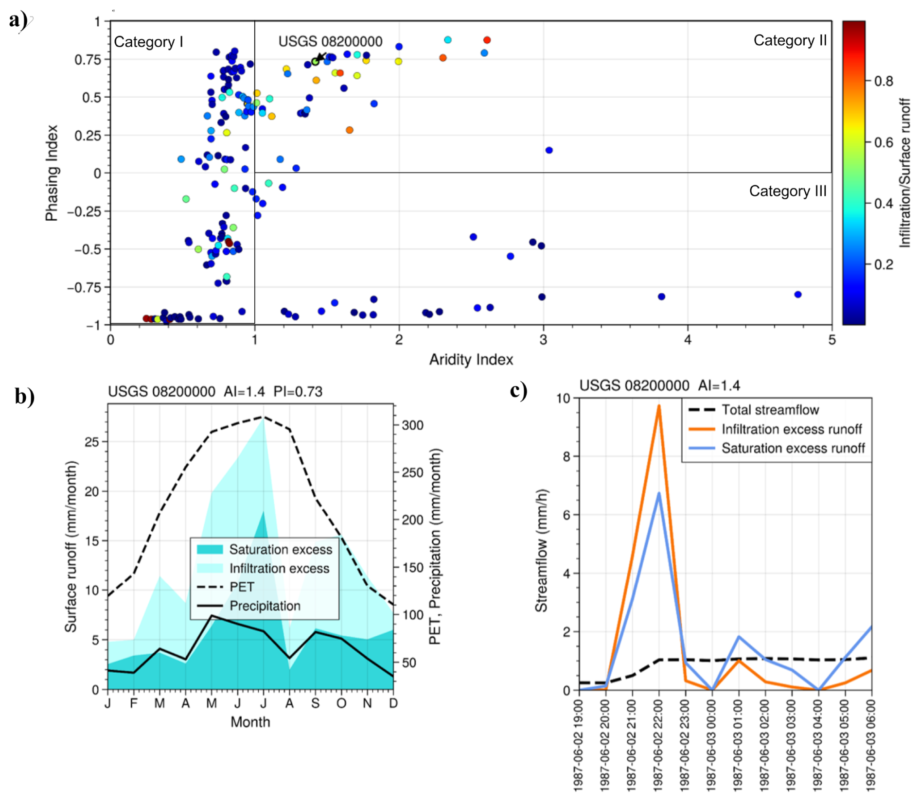
Figure 4 Relative dominance of infiltration and saturation excess runoff at the (a) annual, (b) seasonal, and (c) event scales. (a) includes all the 181 study catchments, (b) and (c) are for a small catchment with its outlet at the USGS station 08200000: Hondo Creek near Tarpley in TX.

Figure 4a depicts the relative dominance of infiltration and saturation excess runoff, expressed in the form of the ratio of annual mean infiltration excess runoff to annual mean total surface runoff, as a function of climate conditions. The climate aridity index (AI), which is the ratio of mean annual potential evapotranspiration (PET) to mean annual precipitation (P), is a classic signature of humid-to-arid climate regimes. The Phasing Index (PI), which is the correlation coefficient between monthly PET and P ranging from −1.0 to 1.0, serves as a signature for seasonal climate conditions (Ye et al., 2017). PI approaching −1.0, 0.0, and 1.0 means that seasonal PET and P cycles are strongly out of phase, not synchronized, and strongly in phase, respectively. Interestingly, despite various combinations of climate and landscape conditions, the hydrologic responses of the 181 catchments can be simplified into only three categories:

•  

  Category I: For the catchments under humid climates (AI ≤ 1.0), saturation excess runoff dominates over infiltration excess runoff due to wet soil status before most storm events.

•  

  Category II: For catchments under arid climates (AI > 1.0) and with monthly PET and P in phase (0 < PI ≤ 1.0), soil is consistently dry and unsaturated within a catchment since PET is always higher than P. Infiltration excess runoff thus likely dominates year-round.

•  

  Category III: For the catchments under arid climates (AI > 1.0) and with monthly PET and P out of phase ($-\mathrm{1.0}<$ PI ≤ 0), there is a sharp distinction between the wet and dry seasons. During the wet season, the monthly PET is obviously lower than the monthly P, and the soil is sufficiently wet, so saturation excess runoff dominates. During the dry season, the monthly PET is significantly higher than the monthly P, and the soil is very dry, resulting in minimal surface runoff. Infiltration excess runoff, nevertheless, may still occur during the dry season under extreme storm events.

Regime curves of P, PET, Ri, and Rs for representative catchments in all three categories are provided in Supplementary Fig. S5. An example of typical Category II catchment is illustrated in Fig. 4b and c. In Fig. 4b, the monthly PET and P values are in phase, with PET consistently higher than P. Infiltration excess runoff accounts for 54 % of the total direct runoff. In Fig. 4c, we zoom into a few consecutive storm events from 2 to 3 June 1987. Infiltration excess runoff was dominant in the initial few hours, e.g., from 21:00 to 22:00 (UTC) on 2 June 1987, and then saturation excess runoff gradually took over. For additional examples in all three categories, please refer to Figs. S5, S6 and S10.

We note that although climate conditions govern surface runoff variations over most catchments, a small number of catchments do not fall within the categories above. These outlier catchments do not exhibit a clear and consistent hydroclimatic pattern, suggesting that additional local controls, such as vegetation dynamics or geological complexity, may influence their runoff behavior. Further investigation of these other factors is beyond the scope of this paper and is left for a future, full-scale study.

4 Summary and Conclusion

This paper has introduced a new runoff scheme, URSSIE, that coherently represents infiltration and saturation runoff generation mechanisms within a single framework. URSSIE effectively accounts for the effects of spatially organized and dynamically evolving soil water storage on both saturation and infiltration excess, as well as their interconnections in both space and time. To demonstrate its effectiveness, we have developed a simple, physically based hydrologic model applicable at the catchment scale, yielding promising performance. It is thus plausible for URSSIE to capture the relative dominance of infiltration and saturation runoff across multiple temporal scales, enabling it to represent the dynamics of surface runoff across catchments spanning a range of climatic and hydrologic conditions.

There are several areas for future explorations, including but not limited to: (1) whether and how URSSIE is applicable at different time scales (e.g., daily or longer), (2) the linkages between landscape conditions (e.g., vegetation dynamics and topographic controls) and the parameterization of infiltration capacity and storage capacity distribution in URSSIE warrant further investigation, (3) the applicability of URSSIE in snow-dominated or managed catchments, (4) incorporating URSSIE in a comprehensive land surface modeling framework and testing it at the catchment and larger scales.

We suggest that URSSIE, as a new method for simulating runoff in hydrologic and land surface models, has profound theoretical promises and broad implications, including but not limited to (1) flood prediction in arid and semi-arid regions due to theoretically more robust surface runoff simulation; (2) coupling between ecological and hydrologic processes due to potentially better estimation of precipitation infiltration hence soil moisture variation; (3) land-atmospheric interactions due to potentially better simulation of soil moisture dynamics. URSSIE will help advance our fundamental and predictive understanding of terrestrial hydrology in land surface and earth system modeling.