Assessing deficiencies in remotely sensed actual evapotranspiration (AET): introducing AET signatures

Hydrological signatures are statistical metrics useful to quantify and infer behaviours of hydrological processes, but there has been limited use of signatures for non-streamflow variables, such as actual evapotranspiration (AET). AET signatures can assist in tasks such as evaluating remotely sensed products, diagnosing deficiencies in hydrological models, and improving understanding of hydrological processes, such as the role of AET in driving hydrological drought. This study focuses on first of these three applications. To achieve this, the study proposes eight AET signatures defined at temporal scales from daily to annual. Two remotely sensed AET (AET_RS) products are assessed against flux tower AET (AET_Fluxtower) at seventeen FluxNET sites in Australia. The two AET_RS products are Moderate Resolution Imaging Spectroradiometer (MODIS,16A2GFv06.1), and CSIRO MODIS Reflectance-based Scaling Evapotranspiration (CMRSET). Annually, median AET_RS closely matches AET_Fluxtower, except in less-arid regions. However, signatures reveal AET_RS largely underestimates the variability of flux tower data at both annual and monthly scales. Other monthly indices are better matched, such as indices of water stress and AET asynchronicity with potential evapotranspiration. However, some metrics are better matched in one product than the other, such as the strength and timing of seasonal fluctuations, with MODIS exhibiting a phase shift. Overall, the signatures reveal that regionally-developed CMRSET outperformed globally-developed MOD16A2GFv061. This study, the first to systematically define AET signatures, offers a way of assessing various aspects of AET dynamics across temporal scales. Furthermore, the case study highlights specific deficiencies in AET_RS and may assist in selecting appropriate AET_RS, including for modelling studies.

1 Introduction

Hydrological signatures are statistical metrics used to quantify hydrological behaviours in catchments and can be used to compare hydrological behaviour across space and time (Addor et al., 2018; McMillan, 2021) and to assess the behavioural fidelity of hydrological model simulations against observations (Gupta et al., 2008). This concept of hydrological signatures to quantify hydrological behaviour was initiated in ecohydrology (e.g., Poff et al., 1997; Richter et al., 1996) to assess changes in flow regimes. Since then, their application has expanded across diverse hydrological domains because of its superiority in characterising underlying hydrological processes encoded in streamflow data, which are governed by watershed characteristics and hydroclimate, rather than being just statistical metrics (McMillan, 2021). These signatures are primarily calculated based on streamflow timeseries and commonly grouped into categories such as flow magnitude, duration, frequency, timing, and rate of change (Olden and Poff, 2003). In modelling, the use of signatures contrasts with commonly used aggregate metrics (e.g., Nash Sutcliffe Efficiency (NSE) or Kling Gupta Efficiency (KGE)), which condense the information of coherence/discrepancy between two timeseries down to a single number (Kiraz et al., 2023; McMillan, 2021). Because signatures retain more detailed information on different (and ideally independent) aspects of the flow regime and may be used to quantify model performance for each separate aspect. Likewise, the associated hydrological processes responsible for each aspect can be separately characterised. In practice, signatures have been widely used to quantify dynamics in hydrological variables and in modelling studies (Araki et al., 2022; Kiraz et al., 2023; McMillan, 2021; Westerberg et al., 2011), while their linking to specific hydrological processes remains an open research question, with a key challenge being the interactions among different processes to produce emergent patterns in observed data (McMillan, 2020).

Although there has been a wide range of hydrological signatures defined for streamflow (McMillan, 2021; Olden and Poff, 2003; Safeeq and Hunsaker, 2016), signatures directly calculated based on other hydrological variables are rare, with some notable exceptions of studies that used the soil moisture and groundwater signatures (e.g., Araki et al., 2022; Heudorfer et al., 2019). Building on this foundation, this study aims to systematically define, compile, and test a list of actual evapotranspiration (AET) signatures. These AET signatures are intended to uncover underlying processes, such as hydrological and ecohydrological processes embedded within AET dynamics, which, to our knowledge, have not previously been done. This complements existing literature that investigated various aspects of AET and quantifying it in different study areas, examining at different spatial scales, such as in-situ level (e.g., Rungee et al., 2019), grid level (i.e., remote sensing, e.g., Zhang et al., 2010), catchment level (e.g., Avanzi et al., 2020), and regional level (e.g., Gardiya Weligamage et al., 2023). Moreover, some studies have used streamflow-based signatures such as total runoff ratio (e.g., McMillan et al., 2014; Safeeq and Hunsaker, 2016), streamflow seasonality (e.g., Wrede et al., 2015), and diurnal cycles in streamflow (e.g., Schwab et al., 2016; Wondzell et al., 2010) to examine AET processes, although these signatures are only indirectly related to those AET processes. Furthermore, McMillan (2020) confirms that none of these streamflow-based signatures have investigated AET processes at shorter temporal scales, such as the event scale.

We envisage at least three potential uses for AET signatures, namely (1) assessing the quality of remotely sensed AET products, (2) diagnosing deficiencies in hydrological models, and (3) improving understanding of hydrological processes. Assessment of the quality of remotely sensed AET products is important as these products are widely used across many research areas due to their ability to provide mostly continuous spatiotemporal data, unlike flux tower measurements (Yan et al., 2018; Zhang et al., 2016). However, their capacity to accurately predict various aspects of AET behaviour is often minimally assessed when incorporating them into a modelling study, and AET signatures can provide a more informative assessment. Secondly, AET signatures can be employed to diagnose deficiencies in hydrological models, as the poor representation of AET could significantly impact streamflow predictions, particularly under changing climatic conditions such as climate change or multiyear droughts (Araki et al., 2022; Koster and Suarez, 2001; Peterson and Fulton, 2019). Thirdly, as noted by McMillan (2020), signatures permit the extraction of “meaningful information about watershed processes”, and it is often possible to define signatures to specifically provide information about a process of interest. This is particularly relevant since AET is the second largest water balance component globally (after precipitation). Moreover, recent studies suggest that AET is a contributing cause to changes in rainfall-runoff relationship for the same streamflow under multiyear drought at both annual and seasonal scales (Gardiya Weligamage et al., 2023; Peterson et al., 2021).

Highlighting the importance of using AET signatures, in this paper, we define a set of AET signatures and demonstrate their use in one of the three specific contexts listed above, namely the evaluation of remotely sensed products of AET. We define distinct AET signatures for various temporal scales to best capture AET characteristics relevant to each timescale. Using AET signatures, two remotely sensed products are evaluated against flux tower data at several sites covering different climatic regions in Australia.

2 Material and Methods

Given that the primary purpose of this paper is to introduce a set of signatures for actual evapotranspiration, we begin this section by describing and defining the signatures themselves. This is followed by descriptions relevant to the case study, including the study area, data, and specific methods to utilise the signatures in this case.

2.1 Proposed set of signatures

We propose eight signatures to quantify AET behaviour, as outlined in Fig. 1. This list is not intended to be exhaustive, but rather to seek a set that is reasonably representative of the variety of characteristics inherent to AET dynamics as a good starting point for future research. As with streamflow signatures, the metrics cover a wide range of timescales, and different metrics require different temporal aggregations of AET information (specifically daily, monthly, or annual) tailored to the metric in question.

Figure 1 AET signatures.

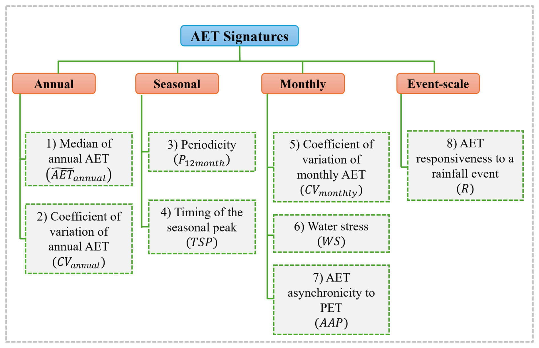
2.1.1 Median of annual AET

To characterise long-term AET, the median of annual AET (${\stackrel{\mathrm{̃}}{\text{AET}}}_{\text{annual}}$) is quantified instead of mean, because the median is less sensitive to occasional extreme values/outliers and therefore provides a more robust estimate of central tendency for comparison across sites.

2.1.2 Coefficient of variation of annual AET

Here, interannual variability is expressed as the coefficient of variation of annual AET (CV_annual). We adopt CV rather than absolute variability measures (e.g., variance, standard deviation, or interquartile range) deliberately following streamflow signature studies such as Clausen and Biggs (2000), as it facilitates the comparison of variability across sites with different means.

$$\begin{array}{}\text{(1)}& {\text{CV}}_{\text{annual}}={\displaystyle \frac{s_{\text{AET}}}{\stackrel{\mathrm{‾}}{\text{AET}}}}\end{array}$$

where s_AET is the sample standard deviation of annual AET, and $\stackrel{\mathrm{‾}}{\text{AET}}$ is the mean annual AET

2.1.3 Periodicity

The periodicity (P_12month) in this study quantifies the tendency for AET variation to recur with the seasonal cycle, i.e., with a period of 12 months, and as such, is calculated as the lag-12 autocorrelation of monthly AET. This will be unity in cases where the timeseries data varies with a perfectly repeating seasonal cycle.

2.1.4 Timing of seasonal peak

The timing of the seasonal peak (TSP) is determined from monthly timestep data by examining the median AET for each of the 12 calendar months and identifying the month with the maximum median AET. Note that the selection of median over mean AET is intended to minimize the influence of extreme values.

2.1.5 Coefficient of variation of monthly AET

The intra-annual (monthly) variability is quantified using coefficient of variation of monthly AET (CV_monthly)

$$\begin{array}{}\text{(2)}& {\text{CV}}_{\text{monthly}}={\displaystyle \frac{s_{\text{AET}}}{\stackrel{\mathrm{‾}}{\text{AET}}}}\end{array}$$

where s_AET is the sample standard deviation of monthly AET, and $\stackrel{\mathrm{‾}}{\text{AET}}$ is the mean monthly AET

2.1.6 Water stress

We define two signatures related to water stress (WS), with the idea that the absence of water stress leads to AET perfectly mimicking potential evapotranspiration (PET). When AET deviates from PET, it marks a deficit in water availability, which may be temporary (e.g., seasonal) or prolonged (as would be seen in arid environments). Both water stress indices assume that the user has access to a timeseries of estimated PET.

Water stress is defined as the difference between average monthly PET and average monthly AET, divided by the average monthly PET. Thus, higher values of this water stress signature indicate less rainfall and/or high PET. Initial testing revealed this metric to be very sensitive to aridity, since it is obvious that AET will be much less than PET in arid areas. In non-arid areas, there might arise temporary (seasonal) water deficits that are not well characterised by the first water stress metric.

$$\begin{array}{}\text{(3)}& \text{WS}={\displaystyle \frac{\stackrel{\mathrm{‾}}{\text{PET}}-\stackrel{\mathrm{‾}}{\text{AET}}}{\stackrel{\mathrm{‾}}{\text{PET}}}}\end{array}$$

where $\stackrel{\mathrm{‾}}{\text{PET}}$ and $\stackrel{\mathrm{‾}}{\text{AET}}$ represent the mean monthly potential evapotranspiration and mean monthly actual evapotranspiration, respectively.

2.1.7 AET asynchronicity to PET

AET asynchronicity to PET (AAP) is defined to capture temporary fluctuations in water stress and is purely based on the asynchronicity between normalised PET and AET. Conceptually, AAP can be thought of as quantifying the area between the normalised curves. To compute this signature, PET and AET monthly timeseries are first normalised by dividing them by their mean monthly PET and AET values, respectively. Then, the numerator is calculated by applying the trapezoidal rule to the absolute difference between normalised monthly PET and AET. Taking the absolute difference between values in the numerator captures the degree of asynchronicity between AET and PET curves, regardless of which of the curves happens to be greater at the given point in time. The denominator of the metric is then similarly calculated by the trapezoidal rule applied to the maximum value among normalised PET and AET at each monthly time step.

$$\begin{array}{}\text{(4)}& \text{AAP}={\displaystyle \frac{{\sum }_{i=\mathrm{1}}^{n-\mathrm{1}}\frac{\mathrm{1}}{\mathrm{2}}\left(\right|E_i-A_i|+|E_{i+\mathrm{1}}-A_{i+\mathrm{1}}\left|\right)}{{\sum }_{i=\mathrm{1}}^{n-\mathrm{1}}\frac{\mathrm{1}}{\mathrm{2}}\left(\text{max}\right(E_i,A_i)+max(E_{i+\mathrm{1}},A_{i+\mathrm{1}}\left)\right)}}\end{array}$$

where E is the normalised monthly PET and A is the normalised monthly AET, and i is the monthly timestep

2.1.8 AET responsiveness to a rainfall event

The event scale is also important, even though it is assessable only for certain data types (e.g., flux tower data; simulations from daily timestep models) and not others (e.g., remotely sensed information provided on timesteps greater than a day). To assess AET dynamics at the event scale, we explored several options to quantify AET responsiveness to a rainfall event – in other words, the degree to which a rainfall event causes a jump in AET. However, the difficulty of such a metric is that rainfall events may not only influence AET on the given day but also influence AET in the following days. If so, a standard correlation measure would be insufficient, but a lagged correlation is difficult to define since we do not know the lag a priori (and it may change over time). Seeking a generalisable metric, we select rainfall events greater than a threshold and identified the maximum daily AET value after the given rainfall event, up to a certain window duration (in days) after that event. We then apply a standard linear correlation equation to the anomalies of these ordered pairs of numbers (i.e., rainfall anomaly versus maximum AET anomaly in the window after the rainfall event). Since this formulation is different from commonly used correlation metrics, we call it simply the “AET responsiveness to a rainfall event” (R). For the purposes of the demonstration, we subjectively set the rainfall threshold and window duration parameters as 5 mm d⁻¹ and 10 d, respectively. It is noted that this window size is also sensitive to the gap between selected rainfall events. If two rainfall events exceeding 5 mm d⁻¹ occurred within the 10 d window period, the window size is restricted to the days between the two rainfall events, and the maximum AET value was chosen from that restricted window.

$$\begin{array}{}\text{(5)}& R={\displaystyle \frac{{\sum }_{i=\mathrm{1}}^n{P}_i^{\prime }\cdot {\text{AET}}_i^{\prime }}{\sqrt{{\sum }_{i=\mathrm{1}}^n{P}_i^{\prime \mathrm{2}}{\sum }_{i=\mathrm{1}}^n{\text{AET}}_i^{\prime \mathrm{2}}}}}\end{array}$$

where, i indexes rainfall events which exceed the predefined rainfall threshold. $P_i^{\prime }$ is the rainfall anomaly for event i, defined as:

$$\begin{array}{}\text{(5a)}& P_i^{\prime }=P_i-\stackrel{\mathrm{‾}}{P}\end{array}$$

with P_i is the rainfall depth of event i, and $\stackrel{\mathrm{‾}}{P}$ is the mean rainfall calculated from all the selected events exceeding the predefined rainfall threshold.
${\text{AET}}_i^{\prime }$ is the AET anomaly associated with the rainfall event i, defined as:

$$\begin{array}{}\text{(5b)}& {\text{AET}}_i^{\prime }={\text{AET}}_{i+j}-\stackrel{\mathrm{‾}}{\text{AET}}\end{array}$$

j is the lag (in days) at which the maximum AET occurs after rainfall event i, with $\mathrm{0}\le j\le \mathrm{10}$ in this study
AET_i+j is the maximum daily AET observed within a window of up to j days after rainfall event P_i, and
$\stackrel{\mathrm{‾}}{\text{AET}}$ is the mean of maximum AET observed across all the events.

2.2 Study Area

Relative to global averages, Australia is a dry continent with annual average precipitation below 450 mm yr⁻¹ (Isaac et al., 2017). However, the coastal areas from southeast Australia to northern Australia receive comparatively higher precipitation, exceeding 1000 mm yr⁻¹ in many areas. This study focuses on seventeen OzFlux sites in Australia (Fig. 2). OzFlux, a part of the international FluxNET program, is a micrometeorological monitoring network in Australia and New Zealand equipped with eddy covariance measurements, providing information on carbon, energy, and water exchange. The seventeen sites constitute the majority of flux towers in Australia; while seven other active flux towers exist, they were excluded due to insufficient coverage (i.e., <7 years) and considerable percentages of negative and unavailable data. The selected study sites cover a wide range of climate and ecosystem regions in Australia, as summarised in Table 1. The time period of data availability varies at each site (typically 7–20 years). Hence, different periods of data coverage are adopted in this study to perform the analysis at each site.

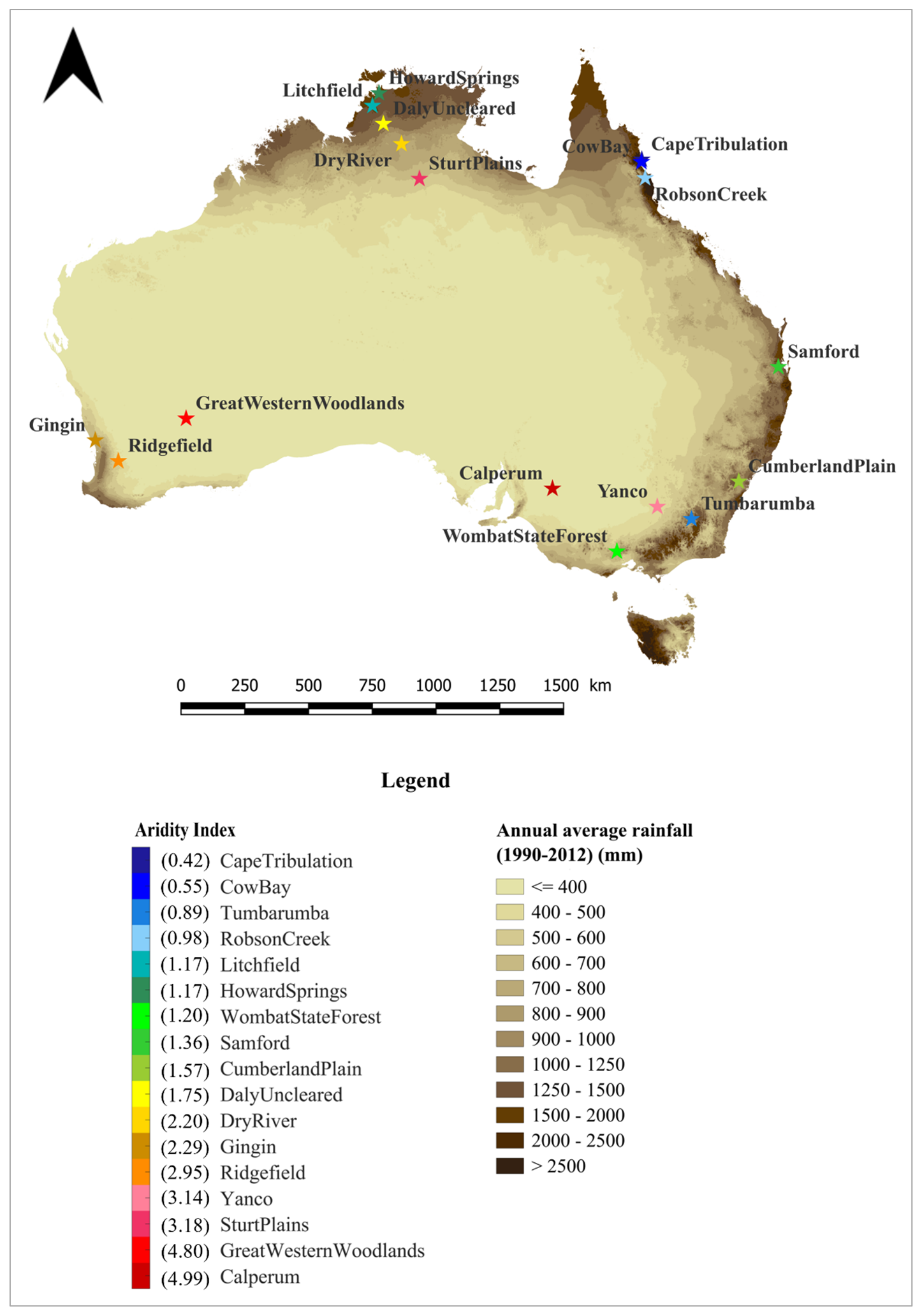
Figure 2 Locations of selected OzFlux sites in this study (Note that the flux tower sites are marked based on the aridity index).

Table 1 Summary of OzFlux sites.

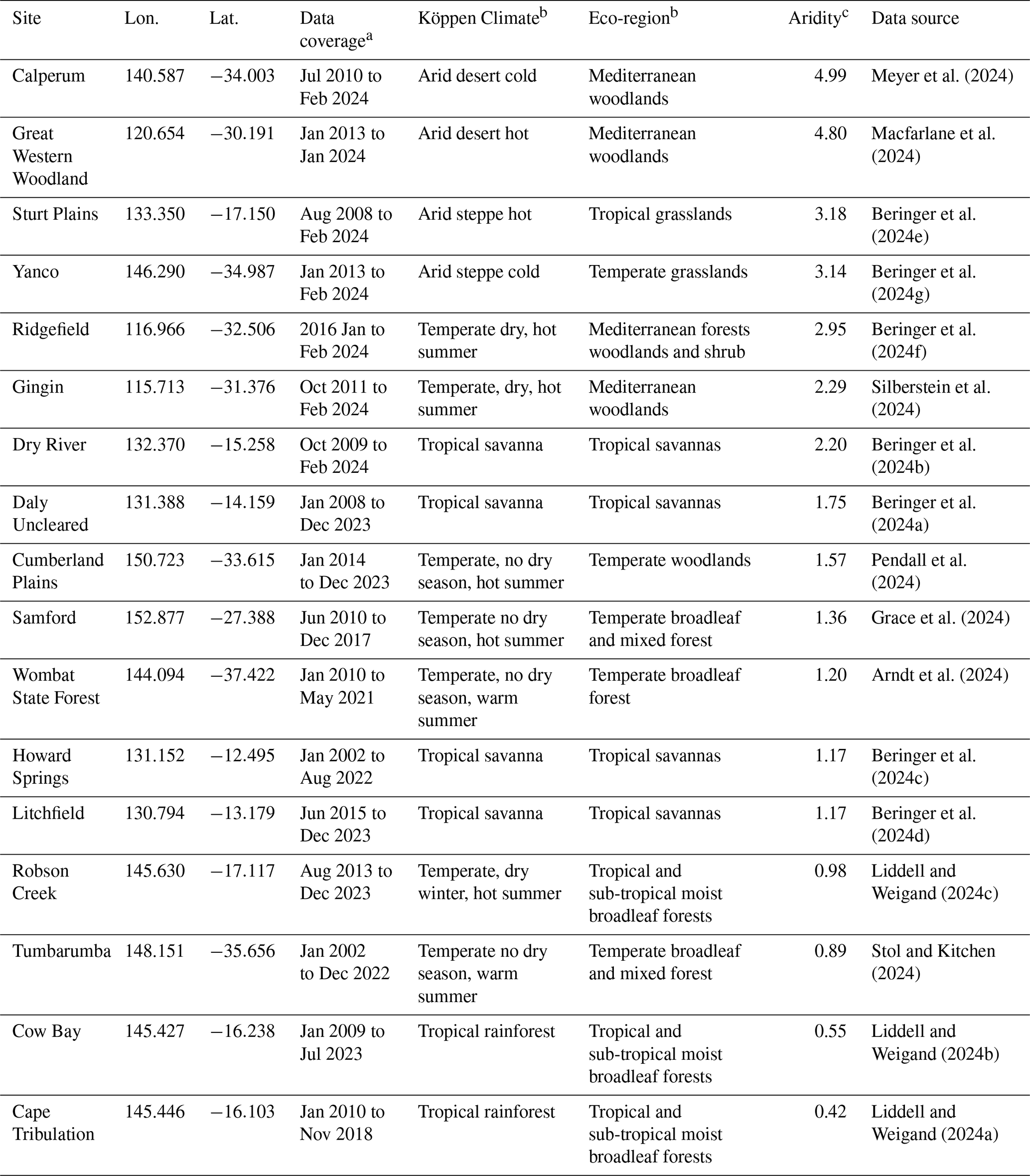
^a This study used version 1 of the year 2024 (2024_V1) of flux tower data from TERN data portal.
^b Guerschman et al. (2022).
^c Aridity refers to the aridity index defined as the ratio of potential evapotranspiration (PET) to precipitation (P).

2.3 Data

2.3.1 OzFlux eddy covariance evapotranspiration data

AET data, version 1 of the year 2024 (2024_V1), were obtained from OzFlux towers through the Terrestrial Ecosystem Research Network (TERN) data portal (https://portal.tern.org.au/, last access: 30 April 2024) at daily, monthly, and annual time scales. To minimize variability among sites due to different processing steps, the data providers consistently apply PyFluxPro (v3.4.17) to implement a standardized method to process data, as described in Isaac et al. (2017). Level 6 flux tower data, adopted here, undergoes quality control, gap filling, and partitioning of the net ecosystem exchange of carbon data into gross primary production and ecosystem respiration. We conducted further data quality checks of the daily AET data and filtered out negative daily AET values. The maximum percentage of negative daily AET values among seventeen study sites was less than 2.3 %.

2.3.2 Remotely sensed evapotranspiration data

Remotely sensed AET (AET_RS) products are popular due to the relative rarity of flux towers and because they provide spatially distributed data, in contrast to flux tower data, which are near-point scale. Here, we present an example of the application of AET signatures to examine two AET_RS products to assess their ability to capture different aspects of AET behaviours at various temporal scales. The two AET_RS products are (1) Pixel resolution 500 m, gap filled, 8 d composites of version 6.1 of Moderate Resolution Imaging Spectroradiometer (MOD16A2GF.061) from Running et al. (2021), referred to as “MODIS AET” hereafter, and (2) 30 m high-resolution, monthly composites of CSIRO MODIS Reflectance-based Scaling Evapotranspiration (CMRSET) from McVicar et al. (2022). The MODIS AET product is one of the most widely used global AET datasets in hydrological and biogeochemical studies (e.g., Baker et al., 2021; Gaona et al., 2022; Salazar-Martínez et al., 2022), while CMRSET is an Australian regional product tested and used extensively over the corresponding region (e.g., Doody et al., 2023; Guerschman et al., 2022; Xu et al., 2022). In both cases, we extracted AET timeseries from pixels that contain the flux tower sites. The 8 d composites of MODIS AET data were aggregated into monthly data through weighted temporal averaging.

2.3.3 Potential evapotranspiration data

As water stress and AET asynchronicity to PET require a timeseries of PET, they were quantified using monthly Morton's wet environment potential evapotranspiration (Morton, 1983; Eq. 61) from the SILO (Scientific Information for Land Owners) database (https://www.longpaddock.qld.gov.au/silo/, last access: 30 April 2024).

$$\begin{array}{}\text{(6)}& M_{\text{wet}}=b_{\mathrm{1}}+b_{\mathrm{2}}{\left(\mathrm{1}+{\displaystyle \frac{{\mathit{\gamma }}_p}{{\mathrm{\Delta }}_p}}\right)}^{-\mathrm{1}}{R}_{\text{TP}}\end{array}$$

where, b₁, b₂ – Empirical constants, Δ_p – slope of saturation vapour pressure at equilibrium temperature (T_P), R_TP – net radiation for land surface at T_P.

2.4 Method

To characterise the performance of AET_RS products, the signatures described in Sect. 2.1 are calculated separately for flux towers AET (AET_Fluxtower) and AET_RS. Then, we investigated the deviation of AET_RS signatures from AET_Fluxtower signatures. As mentioned above, different periods have been considered at each flux tower site depending on their data coverage. For each site, the flux tower period of record determined the period of comparison between flux tower and remotely sensed information. Finally, the traditional efficiency metrics such as NSE (Nash and Sutcliffe, 1970; Eq. 7), KGE (Gupta et al., 2009; Eq. 8), and components of KGE were calculated using monthly MODIS and CMRSET AET at each flux tower site. These metrics are often relied upon by authors to characterise quality of timeseries data but the downside is that they have limited capabilities of demonstrating what aspects of dynamics is deficient in the case of a low performance score. Here we demonstrate that the signatures can be used to contextualise low scores at some sites, where traditional metrics are deficient.

It is important to clarify that these efficiency metrics are calculated over time at individual sites. For instance, NSE is computed at each site across time, which differs from the use of NSE to assess the agreement of signature values across multiple sites between AET_RS and AET_Fluxtower. To avoid confusion, we refer to the former as NSE_{across time, single site}, and the latter as NSE_MODIS and NSE_CMRSET, which denote how well the remotely sensed AET signatures match the flux tower-derived signatures across sites.

$$\begin{array}{}\text{(7)}& \text{NSE}=\mathrm{1}-{\displaystyle \frac{{\sum }_{i=\mathrm{1}}^n({\text{AET}}_{\text{Fluxtower},i}-{\text{AET}}_{\text{Rs},i}{)}^{\mathrm{2}}}{{\sum }_{i=\mathrm{1}}^n({\text{AET}}_{\text{Fluxtower},i}-\stackrel{\mathrm{‾}}{{\text{AET}}_{\text{Fluxtower}}}{)}^{\mathrm{2}}}}\end{array}$$

where, i – time step (in the case of NSE calculation across time at a single site), AET_Fluxtower,i – Flux tower AET at i, AET_Rs,i – Remotely sensed AET at i, $\stackrel{\mathrm{‾}}{{\text{AET}}_{\text{Fluxtower}}}$ – Mean of flux tower AET, n – Number of observations.

$$\begin{array}{}\text{(8)}& \text{KGE}=\mathrm{1}-\sqrt{(r-\mathrm{1}{)}^{\mathrm{2}}+(\mathit{\alpha }-\mathrm{1}{)}^{\mathrm{2}}+(\mathit{\beta }-\mathrm{1}{)}^{\mathrm{2}}}\end{array}$$

where, r – Pearson correlation coefficient between flux tower and RS AET, α – Ratio of standard deviation between RS AET and flux tower, β – Ratio of mean between RS AET and flux tower.

3 Results

The AET signature results are presented in the four main categories based on the temporal scales in the order of (1) annual, (2) seasonal, (3) monthly, and (4) event-scale. To allow better contextualisation of AET signature results, we first present some example monthly timeseries plots of AET_Fluxtower, AET_RS, SILO rainfall, and PET at six flux towers (Fig. 3). These timeseries plots highlight some aspects of AET that can be observed through visual inspections, such as AET variability, periodicity, and asynchronicity between AET and PET. For example, notable variability is observed in both AET_Fluxtower, AET_RS at Wombat State Forest and Howard Springs. In Gingin, seasonal variations in AET_Fluxtower appear to be offset from PET, indicating asynchronicity. In Robson Creek, lower temporal variability in AET_Fluxtower, is observed compared to AET_RS. These kinds of dynamics can be systematically examined and quantified using AET signature results.

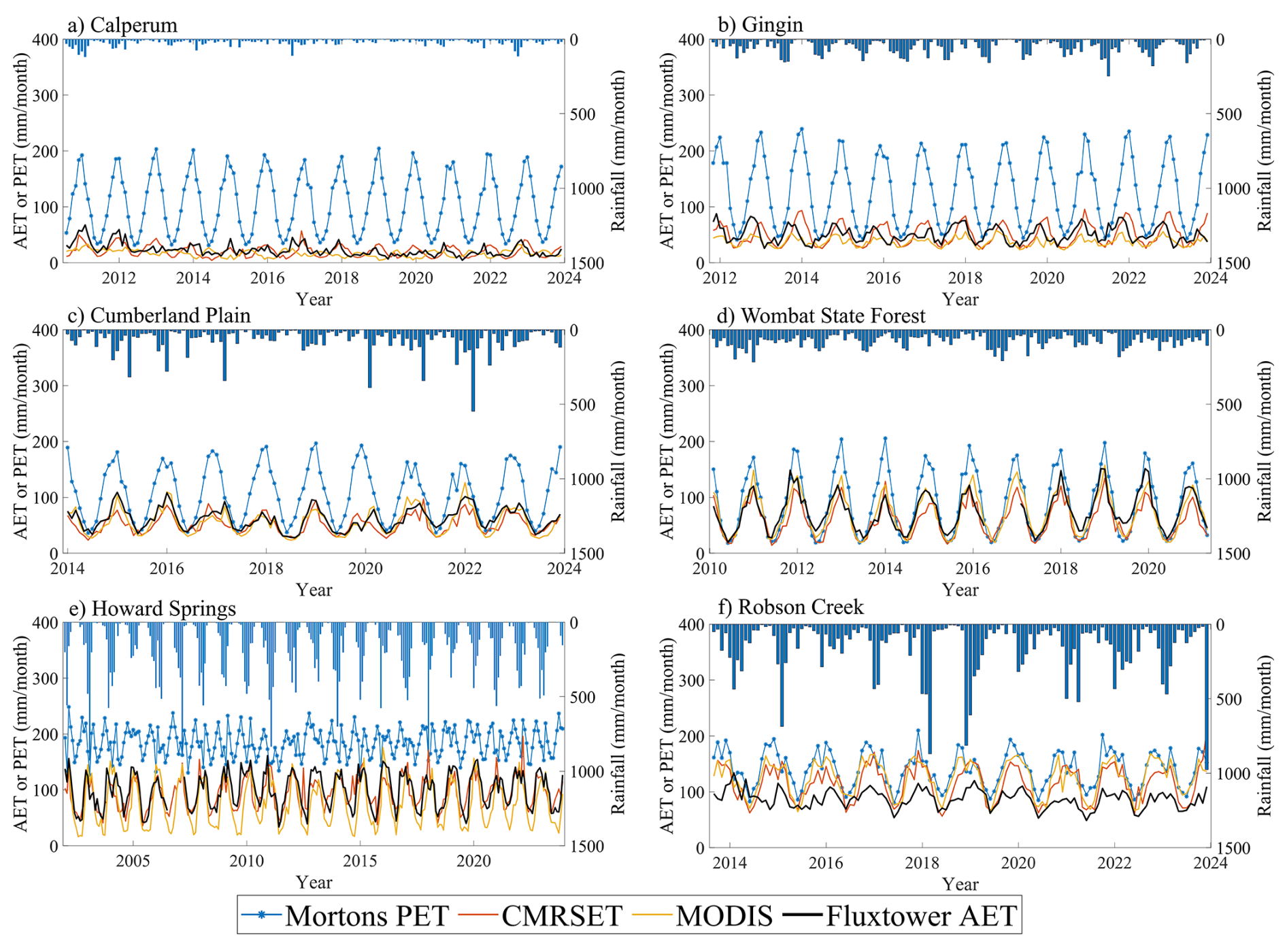
Figure 3 Monthly timeseries plots of flux tower and remotely sensed AET, rainfall and PET at six example flux tower sites.

3.1 Annual AET signatures

Figure 4a shows an increase in the long-term median (${\stackrel{\mathrm{̃}}{\text{AET}}}_{\text{annual}}$) values with decreasing aridity index, as expected. For example, less arid sites (shown in blues), such as Cape Tribulation and Cow Bay, have higher ${\stackrel{\mathrm{̃}}{\text{AET}}}_{\text{annual}}$, while more arid sites (shown in reds), such as Calperum and Great Western Woodland have lower ${\stackrel{\mathrm{̃}}{\text{AET}}}_{\text{annual}}$. The comparison of ${\stackrel{\mathrm{̃}}{\text{AET}}}_{\text{annual}}$ between flux tower and RS products shows that all sites except for three sites (i.e., Robson Creek, Cow Bay and Cape Tribulation) in the tropical northern Queensland, the RS ${\stackrel{\mathrm{̃}}{\text{AET}}}_{\text{annual}}$ aligns relatively close one to one line with flux tower ${\stackrel{\mathrm{̃}}{\text{AET}}}_{\text{annual}}$ (NSE_CMRSET=0.61 and NSE_MODIS=0.42), although some scatter and slight underestimation are evident. In contrast, the three tropical northern Queensland sites, there is a strong overestimation of RS ${\stackrel{\mathrm{̃}}{\text{AET}}}_{\text{annual}}$, despite differences in aridity among these sites. Figure 4b shows a higher coefficient of variation of annual AET (CV_annual) at arid flux tower sites such as Calperum, Sturt Plains, and Yanco, whereas other sites show lower CV_annual within the range of 0–0.2. CV_annual is lower in both MODIS and CMRSET AET compared to flux towers at almost all flux towers, and the scatter is high.

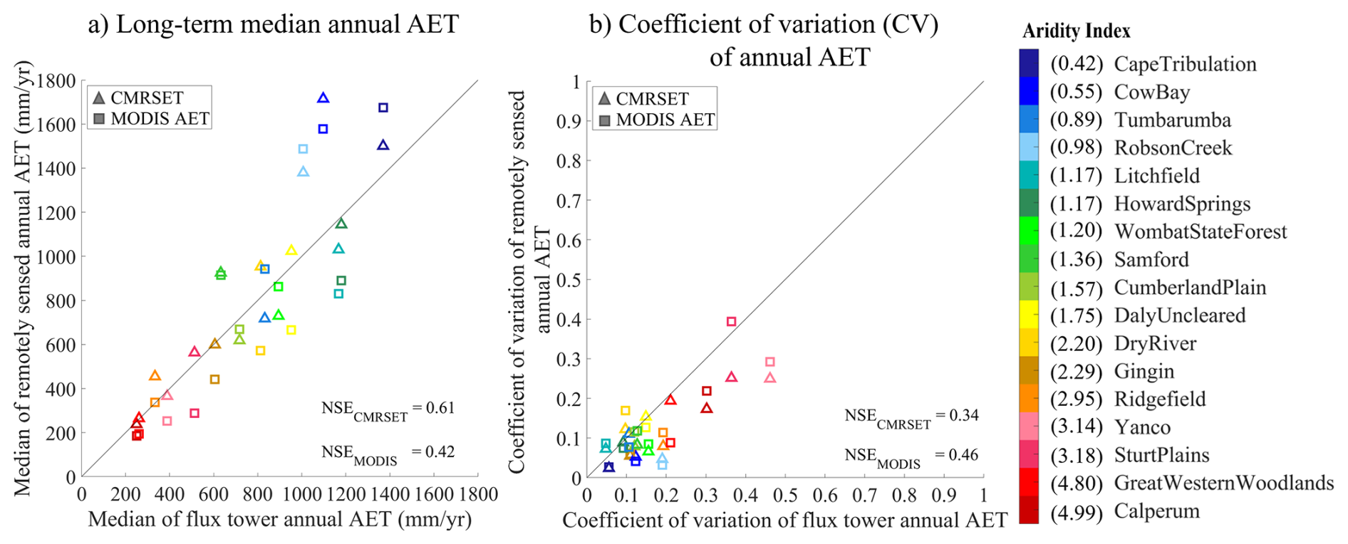
Figure 4 Comparison of annual AET signatures; (a) Long-term median AET, (b) Coefficient of variation (CV) of annual AET, between remotely sensed AET (MODIS and CMRSET AET) and flux tower AET. (Note that the flux towers are ordered by aridity index – from Cape Tribulation (Lowest aridity) to Calperum (Highest aridity)).

3.2 Seasonal AET signatures

Figure 5a shows periodicity (P_12month) via the lag-12 autocorrelation. No clear relationship is observed in P_12month with aridity. For example, weaker P_12month values are observed at both the more arid flux tower sites (e.g., Great Western Woodlands, Yanco) and less arid flux tower sites (e.g., Cape Tribulation). Remotely sensed data performs more poorly in this metric than in any other. Across all sites, the P_12month of CMRSET monthly AET does not systematically over- or underestimate flux tower P_12month. However, there is a considerable scatter meaning some sites showing significant overestimation and others significant underestimation of CMRSET P_12month to flux tower P_12month. In contrast, MODIS monthly AET shows stronger periodic behaviour than ground measurements at most of the flux tower sites.

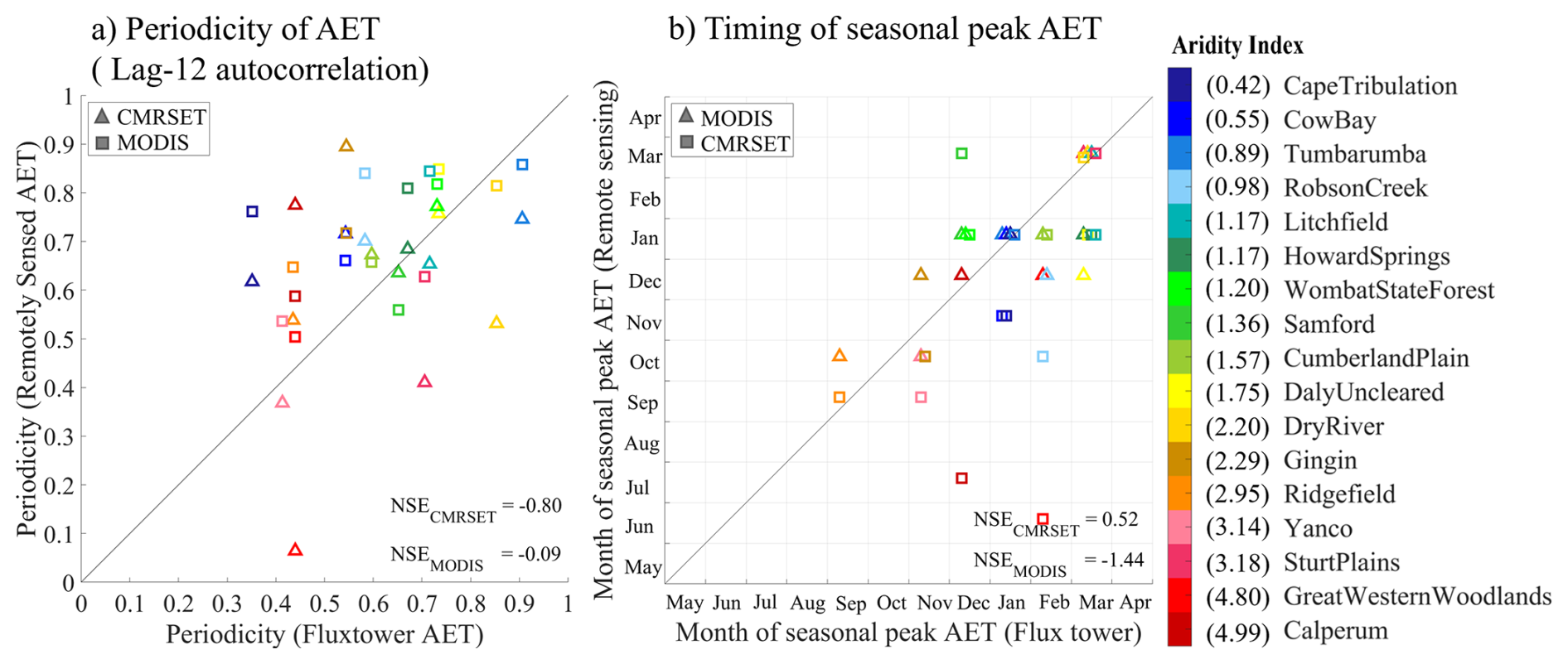
Figure 5 Comparison of seasonal AET signatures, (a) Periodicity of AET (Lag-12 autocorrelation), (b) Timing of seasonal peak, between remotely sensed AET (MODIS and CMRSET AET) and flux tower AET. Note that Fig. 5b values take integer values only (i.e., either one calendar month or the next), leading to several points overlying the same plotting position; to make every point visible we subject each point to a jitter (i.e., a unique offset within the same grid cell).

Figure 5b compares the timing of seasonal peaks (TSP) between AET_RS and AET_Fluxtower estimates. Here, CMRSET tends to show the same timing (7 out of 17 flux towers) or closer timing (e.g., one month offset – 6 out of 17 flux towers) of TSP as flux towers at many flux tower sites, whereas those calculated using MODIS AET are significantly offset with flux tower TSP.

3.3 Monthly AET signatures

Figure 6 quantifies and compares monthly AET signatures using AET_Fluxtower and AET_RS. Figure 6a shows a lower CV_monthly at less arid flux towers such as Cape Tribulation, Cow Bay, and Robson Creek, with most other flux towers grouping tightly between CV values of 0.3 and 0.6, while Sturt Plains is a clear outlier at 0.9. CV_monthly from CMRSET and MODIS AET do not show much overall bias relative to AET_Fluxtower, yet the match with observed is very poor, with considerable scatter due to overestimation and underestimation of CV_monthly, depending on site.

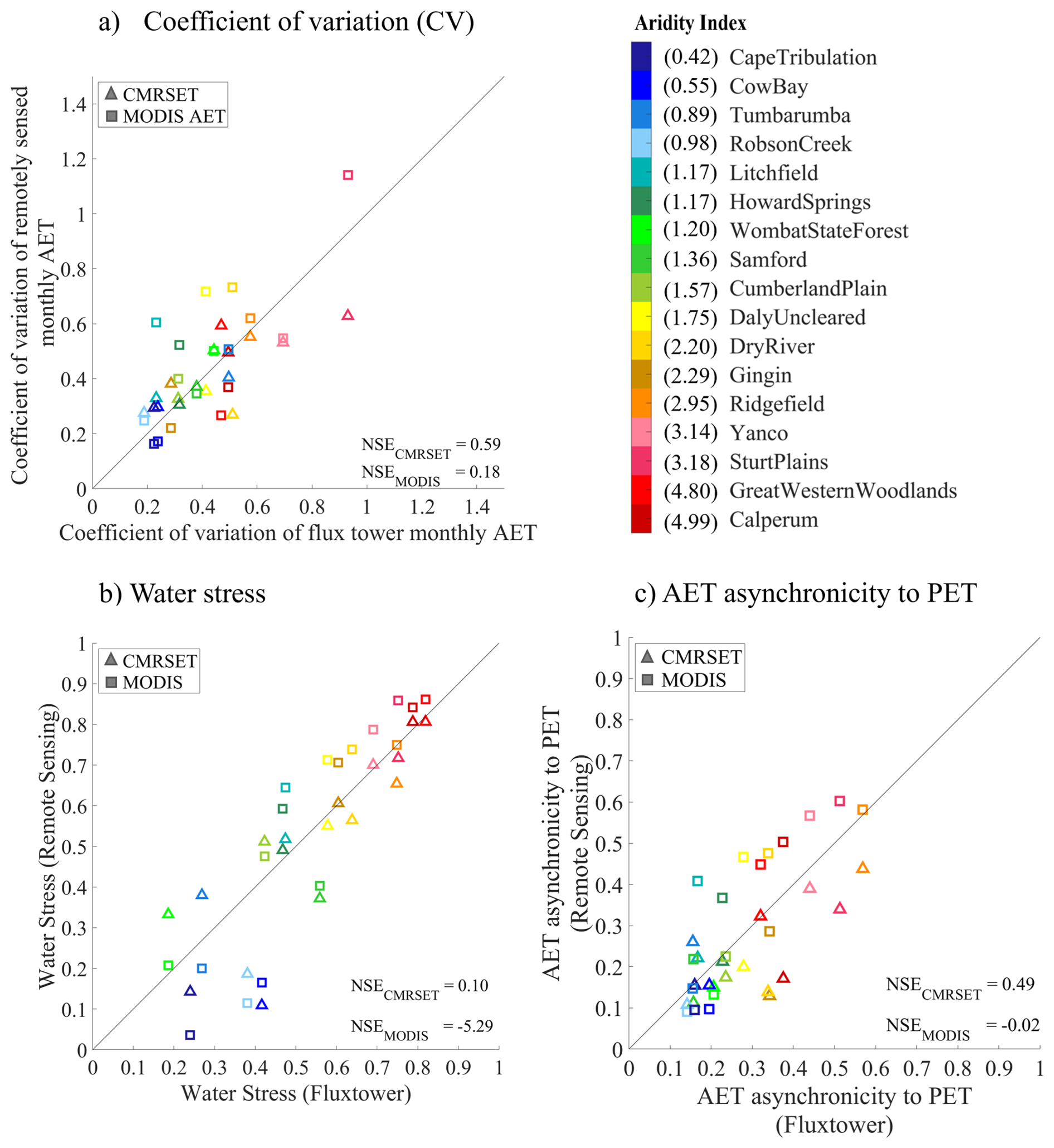
Figure 6 Comparison of monthly signatures; (a) Coefficient of variation of monthly AET, (b) Water stress, and (c) AET asynchronicity to PET, between remotely sensed AET (MODIS and CMRSET) and flux tower AET.

Regarding water stress (WS), Fig. 6b shows how WS increases with aridity, as expected. WS from CMRSET and MODIS AET is moderately well predicted except for wet flux towers, which are underestimated. Figure 6c shows the AET asynchronicity to PET (AAP) that incorporates differences in phases between AET and PET timeseries. Results show that both AET_Fluxtower and AET_RS are asynchronous with PET (i.e., APP>0) for all the sites. However, at wetter sites, AET is more synchronous with PET showing smaller APP values (i.e., smaller APP indicates closer synchronicity to PET), but increasing with aridity index (except at Calperum and Great Western Woodlands sites). Furthermore, the results show separation between remotely sensed products, with MODIS showing more AAP while CMRSET showing lower AAP compared to flux tower AAP for sites exhibiting higher than average asynchronicity.

3.4 Event-scale AET signatures

Figure 7 shows the AET responsiveness to a rainfall event (R). Recall that such information is unavailable for RS data due to its longer timestep. The R of zero indicates no correlation between rainfall event and the subsequent AET, and Fig. 7 shows no discernible correlation between the magnitude of a rainfall event (i.e., >5 mm d⁻¹ in this example) and the subsequent AET on either the rain day or thereafter (i.e., maximum of 10 d window in this example) at the majority of the flux tower sites, and even a slightly negative correlation, perhaps suggesting that rain days might be followed by cloudy weather that suppresses AET.

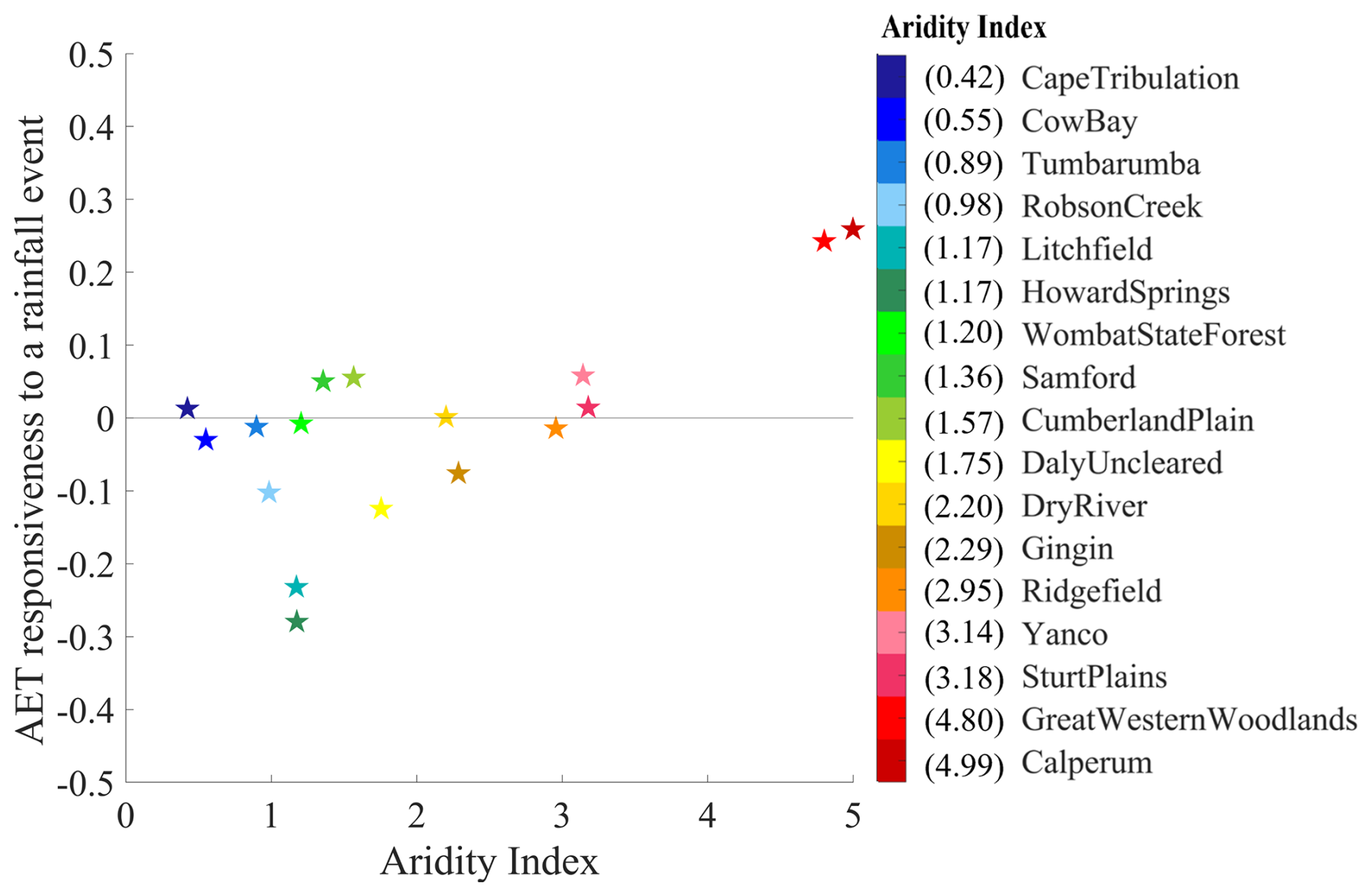
Figure 7 AET responsiveness to rainfall vs. aridity index at flux tower sites. (Note that the index of zero indicates no correlation between rainfall event and the subsequent AET).

3.5 Traditional efficiency metrics

Figure 8 shows a range of commonly used efficiency metrics such as NSE, KGE, and the sub-components of KGE, namely, the ratio of standard deviations (α), the ratio of means (β), and the Pearson correlation coefficient (r), calculated using monthly MODIS and CMRSET AET with flux tower AET. The distribution of NSE (median: −0.11) from MODIS AET indicates a poor prediction of AET_Fluxtower on the monthly scale. In contrast, the distribution of NSE from CMRSET AET shows a positive, but still close to zero, median value of 0.14, implying better performance than MODIS but still overall poor performance.

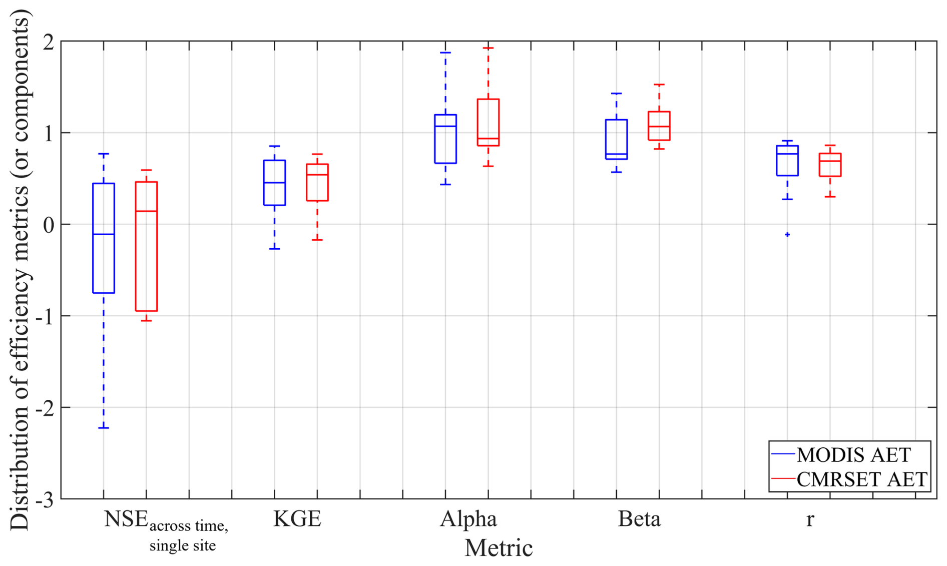
Figure 8 Distribution of conventional efficiency metrics, all calculated on a monthly timestep: (1) Nash Sutcliffe efficiency (NSE_{across time, single site}), (2) Kling Gupta Efficiency (KGE), (3) Alpha (α – ratio of standard deviations), (4) Beta (β – ratio of means), and r (r – Pearson correlation coefficient), calculated using monthly MODIS and CMRSET AET with flux tower AET (Note that there are two outliers not shown in the NSE calculated for MODIS and CMRSET, which are lower than −3).

For KGE, the median KGE values across flux tower sites for monthly MODIS and CMRSET AET are 0.45 and 0.53, respectively. The sub-components of KGE, such as α shows closer variability in MODIS AET (median α=1.07) and in CMRSET (median α=0.94) compared to flux tower estimates. The β component of KGE shows a lower mean in MODIS AET (median β=0.77) and a slightly higher mean in CMRSET (median β=1.07) compared to flux tower estimates. The r component of KGE shows a relatively similar correlation for both MODIS AET (median r=0.77) and CMRSET (median r=0.69) with AET_Fluxtower. Although these components of KGE provide valuable information about the ability of AET_RS to capture dynamics from AET_Fluxtower, this information is diluted in the final KGE value. Figure S1 in the Supplement shows the traditional efficiency metric values at each flux tower site.

4 Discussion

This study developed evapotranspiration signatures at various temporal scales and used them to evaluate remotely sensed AET information against flux towers. The study provides a basis for exploring what sort of signatures might be useful when investigating and characterising AET behaviours, with applications across other domains, such as characterising catchment processes and critiquing hydrological models.

4.1 Value of AET signatures over aggregate measures of performance

AET signatures introduced in this analysis offer behavioural insights into AET to complement existing suites of indices for streamflow and, to a lesser extent, groundwater. A key benefit of these signatures is their capacity to characterise different aspects of AET dynamics, allowing the quantification of nuanced aspects that can be discerned through visual inspection but, without signatures, are not easily defined numerically. Some examples are given in Table 2.

Table 2 Example of aspects of AET dynamics that can be discerned via visual inspection of timeseries (Fig. 3) and are subsequently reflected in signature results (Figs. 5 and 6).

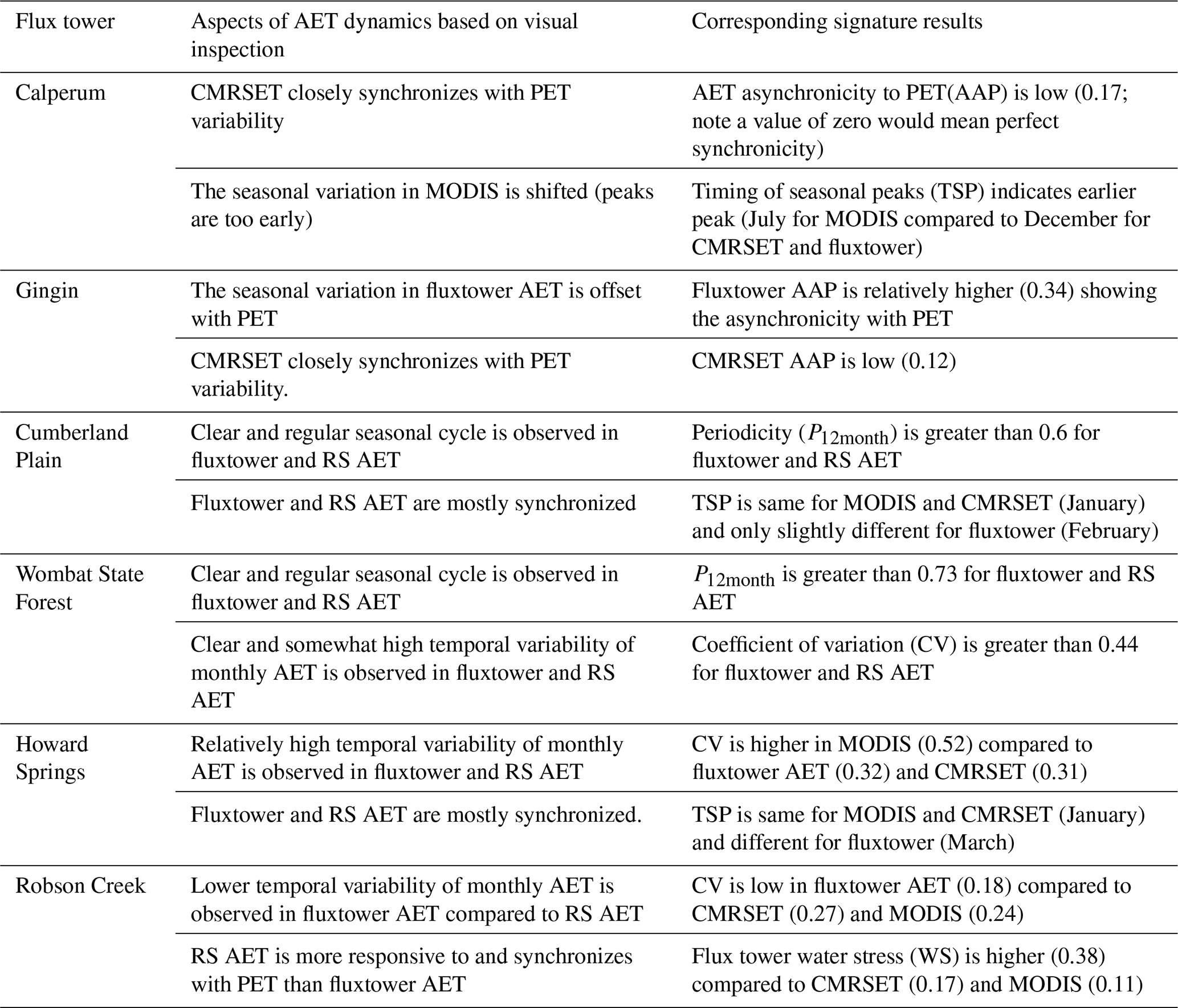
Table 2 provides examples of how observed dynamics in AET, such as variability, seasonality, and the relationship between AET and PET, can be translated into measurable indicators using AET signatures. These signatures enable more objective comparisons between AET_RS and AET_Fluxtower, while also offering insights into the underlying processes within a given region.

This capacity for nuanced characterisation in AET signatures contrasts with traditional fit/performance metrics such as NSE and KGE. As mentioned in the introduction, these commonly used performance metrics are often applied to quantify hydrological model performances, but may obscure specific behavioural information (McMillan, 2021; Wagener and Gupta, 2005). For example, the NSE calculated using monthly MODIS and CMRSET AET at some flux tower sites showed negative values, indicating bad predictive skills, whereas the KGE calculated using both the AET_RS tended to show some predictive skills relative to flux tower observations. However, both of these conventional performance metrics fail to identify which aspects of AET in remote sensing products have led to poor prediction of AET_Fluxtower. For example, as per Table 2, at the arid Calperum site, MODIS AET exhibited an earlier seasonal peak in AET compared to the flux tower, an insight captured by the TSP signature that is unavailable using NSE or KGE. Similarly, at the wet tropical Robson Creek, AET_RS products showed slightly greater monthly variability than flux tower observations, again reflected by CV_monthly signature but not clear in conventional metrics. Even though the subcomponents of KGE, such as the ratio of standard deviation, the ratio of mean, and the Pearson correlation coefficient, provided valuable information about the ability of these two AET_RS products to capture AET dynamics compared to AET_Fluxtower, the final KGE value obscures this information.

Given that AET signatures capture more behavioural information than traditional performance metrics, they can also be used in other applications, such as hydrological modelling for more realistic outcomes, in a similar way to using other hydrological signatures. For example, Huynh et al. (2023) incorporated hydrological signatures into the calibration of a conceptual distributed hydrological model and found improved flash flood predictions, achieving higher NSE and KGE scores compared to models calibrated without signatures. Kiraz et al. (2023) developed a signature-based performance metric that strongly correlated with NSE and KGE, while also enabling calibration and evaluation of regionalised ungauged catchments. Using the AET signatures developed above, Gardiya Weligamage et al. (2025) demonstrated that incorporating AET timeseries data with streamflow information into calibration generally yields improvements in overall model performance, as indicated by NSE and KGE values. Their signature-based assessment of calibration to traditional AET metrics revealed that only the monthly variability and AET synchronicity with PET were enhanced in such calibration (relative to streamflow-only calibration).

While these signatures have many inherent strengths, challenges could remain in applying them, particularly in large sample studies, due to data errors associated with flux tower measurements, particularly in extreme climates (McMillan et al., 2023). Therefore, readers should have a prior understanding when regionalising and interpreting any hydrological behaviours using signatures.

4.2 Insights into actual evapotranspiration behaviour at Australian flux tower sites

Ozflux observations are recognised for their high quality, with minimal data gaps and errors. Isaac et al. (2017) reported that around 80 % of Ozflux sites achieved an energy balance closure ratio exceeding 0.8, indicating robust flux measurements. Moreover, these flux tower sites cover a diverse range of vegetation types, including tropical and temperate grasslands, tropical savannas, Mediterranean and temperate woodlands, and both temperate and tropical forests (Guerschman et al., 2022). Given these high-quality data and broader ecological coverage, this study confirms various anticipated AET behaviours at flux tower sites in Australia across different temporal scales. For example, the ${\stackrel{\mathrm{̃}}{\text{AET}}}_{\text{annual}}$ increased as the aridity index decreased as expected, indicating that less arid flux towers have a higher ${\stackrel{\mathrm{̃}}{\text{AET}}}_{\text{annual}}$, whereas more arid flux towers have a lower ${\stackrel{\mathrm{̃}}{\text{AET}}}_{\text{annual}}$. However, the CV_annual across flux tower sites was low across the majority of sites (range of 0–0.2 at 14 out of 17 sites), regardless of their aridity index. This finding is consistent with the relatively constant annual AET variability over time, as reported by Gardiya Weligamage et al. (2023). The three exceptions were flux tower sites in dry regions such as Calperum, Sturt Plains, and Ridgefield, which exhibited comparatively higher CV_annual (ranging from 0.3–0.5). This is likely driven by high interannual rainfall variability (Liu et al., 2024; Wang et al., 2017) and high PET (Pan et al., 2021) in dry regions. In such regions, evaporation from soil contributes more to AET than transpiration from vegetation in hot arid environments; moreover, vegetation tends to be opportunistic during rainfall events and remains dormant during dry periods (Ratzmann et al., 2016). Therefore, these factors collectively influence the high variability of AET in hot dry regions.

Signatures that capture short-term temporal dynamics of AET, such as CV_monthly, P_12month, and TSP exhibited wide scatter across observed flux tower sites, with no clear relationship to aridity. This decoupling is likely due to the fact that AET dynamics at shorter temporal scales are strongly influenced by local geographic, biophysical, and hydroclimatic conditions such as vegetation dynamics, soil properties, soil moisture dynamics, and inter annual rainfall variability that are not well represented by broad, long-term climate classification like aridity index. van Dijke et al. (2020) reported a strong correlation between leaf area index (LAI) and latent energy (LE) in savanna and arid grassland ecosystems across FluxNet sites, including Ozflux sites. They explained that in these environments, soil water deficiency and high evaporative demand lead to a significant increase in LE even with small increases in LAI. For the evergreen broadleaf forested ecosystem, a positive correlation was also observed between LAI and energy fluxes, attributed to evaporation from canopy interception, which accounts for up to 30 % of total evapotranspiration. While their study suggests that both of these vegetation types exhibit a clear relationship with energy fluxes, our analysis indicates that AET signature patterns, especially on monthly and seasonal scales, cannot be easily explained by classifying based on vegetation cover alone.

At the event scale, most flux towers did not show a discernible correlation between rainfall events and subsequent AET events. Therefore, on first impression, the “AET responsiveness to a rainfall event” signature does not appear to add significant value in this AET signature analysis. However, we could subset event scale rainfall and AET timeseries data by climatic regions, season, or vegetation group to gain more detailed insights. Moreover, we employed this event-scale signature to evaluate commonly used conceptual rainfall-runoff model performances in a companion paper, Gardiya Weligamage et al. (2025), and the models were found to be very biased in this signature, showing simulated AET that was too responsive to precipitation. Therefore, this event-scale signature also adds value in constraining models or exploring model deficiency. Furthermore, this event-scale signature is particularly noteworthy, as it highlights a distinct aspect of AET dynamics not previously quantified. As McMillan (2020) confirmed, no signature (even an indirect AET behaviour explanation using hydrological signatures) was previously identified for assessing AET at the event scale.

4.3 Implications for quality of remotely sensed actual evapotranspiration

The eight AET signatures proposed in this study are used to highlight the strengths and weaknesses of two AET_RS products (i.e., MODIS and CMRSET) on multiple aspects by assessing their AET signatures with those obtained from flux tower observations. Given that it is increasingly common for studies (particularly modelling studies) to adopt AET_RS products, the reported deficiencies in these AET_RS data seem particularly relevant. We emphasize the importance of investigating AET_RS data prior to use in any other applications, such as rainfall-runoff modelling.

While the plots above suggest that AET_RS is generally an unbiased estimate of AET_Fluxtower across the entire catchment sample, the problem is the wide scatter, indicating that estimates at individual sites may be subject to significant errors. This wide scatter was seen in several signatures, such as CV_monthly, AAP, P_12month, and TSP.

At the seasonal scale, notable discrepancy was observed between AET_RS and AET_Fluxtower, in terms of P_12month, and TSP. For example, challenges were more pronounced with the MODIS AET, which exhibited offsets in TSP (NSE${}_{\text{MODIS}}=-\mathrm{1.44}$, see Fig. 5b), while being overly periodic but with scatter compared to flux tower data. This suggests that globally developed MODIS AET often failed to reflect AET dynamics at seasonal scale in diverse Australian environment. Conversely, the regionally developed CMRSET product tended to align comparatively better with the TSP observed by flux towers (NSE_CMRSET=0.52, see Fig. 5b) but with larger scatter. The close alignment of TSP with AET_Fluxtower is likely because the CMRSET model was calibrated only to flux tower sites in Australia (Guerschman et al., 2022), in contrast to MODIS, which is globally calibrated and thus has less Australian focus (Mu et al., 2011). Our findings concur with Guerschman et al. (2022), who reported that the calibrated CMRSET model performs better than MODIS AET (i.e., MOD16A2).

However, Guerschman et al. (2022) also noted that CMRSET captures less of seasonal variability at tropical sites and shows weaker correlation with flux tower AET in arid regions compared to temperate areas. They further explained that the seasonality in tropical and temperate regions is effectively captured by PET, which leads to higher correlation between AET_Fluxtower and CMRSET in those regions than in arid sites. Our results also agree on that higher correlation (r) between both CMRSET (median r=0.69) and MODIS AET (median r=0.77) with flux tower AET. Furthermore, our AAP signature shows that both the AET_RS and AET_Fluxtower with mostly synchronous relationship with PET at flux tower sites in temperate (i.e., flux towers at northern Australia) and tropical regions (i.e., flux towers at northern Queensland).

However, none of the information above supports explaining the differences in periodicity and offsets in seasonal peaks between AET_RS and AET_Fluxtower shown in Fig. 5. We assume that these discrepancies may be attributed to vegetation and surface water stress parameterisation in AET_RS algorithms. However, significant uncertainties related to water stress parameterisation are unlikely, as our assessment using water stress signature showed that water stress is fairly predicted by AET_RS, except for wet, tropical flux tower sites. This exception in the wet tropics could be due to uncertainties associated with the PET (recall that Morton's Wet Environment PET was used in Water Stress signature), which may not be directly comparable to AET_RS. Given this, vegetation parameterisation likely plays a vital role in these observed inconsistencies in P_12month, and TSP. This could be due to uncertainties associated with Enhanced Vegetation Index (EVI) and Global Vegetation Moisture Index (GVMI) in CMRSET and in Leaf Area Index (LAI)/Fraction of Photosynthetically Active Radiation (FPAR) in MODIS. Mu et al. (2011) discussed overestimation of LAI as a potential source of overestimation in MODIS AET. Moreover, MODIS AET applies the same set of biophysical parameters for each biome type globally (Mu et al., 2011). Since Australia has distinct biome types, MODIS AET could introduce uncertainties due to differences in plant biophysics. Gan et al. (2018) also reported MODIS AET underestimates flux tower AET at non-forested sites (e.g., Dry River, Howard Springs, Sturt Plains), but overestimates at forested sites (e.g., Tumbarumba, and Wombat State Forests). Consequently, combined uncertainties and limitations could contribute to the seasonality issues in CMRSET and MODIS AET. Therefore, caution should be exercised when extracting seasonal information from both MODIS AET and CMRSET.

At the annual scale, RS ${\stackrel{\mathrm{̃}}{\text{AET}}}_{\text{annual}}$ largely matched with the flux tower ${\stackrel{\mathrm{̃}}{\text{AET}}}_{\text{annual}}$, although some scatter and slight underestimation were observed. However, a notable overestimation of RS ${\stackrel{\mathrm{̃}}{\text{AET}}}_{\text{annual}}$ was shown at 3 tropical study sites in northern Queensland, namely Robson Creek, Cow Bay and Cape Tribulation. This discrepancy may reflect geographic and hydroclimatic influences specific to these coastal rainforest environments. This includes steep spatial gradients in wetness that may not be well characterised by gridded data, as supported by Guerschman et al. (2022) who also noted the near coast and strong orographic precipitation gradient in the Cow Bay and Cape Tribulation area. This highlights the need for caution when interpreting remotely sensed annual AET in similar settings. In the comparison of CMRSET and MODIS AET, Mohammadi et al. (2015) showed that MODIS AET tends to underestimate in arid floodplains in Australia, similar to several other studies (e.g., Kim et al., 2012; Tang et al., 2015), together suggesting that the underestimation may be due to limitations in MODIS AET in estimating land cover changes and water cover fraction. This finding is in line with our results at most flux tower sites. However, our study shows that both the AET_RS underestimate compared to flux tower AET. This could be due to the difference in spatial footprints between AET_RS and AET_Fluxtower. In addition, all CV_annual showed underestimation (negative bias) relative to flux towers, implying relatively poor year-to-year variability in MODIS AET and CMRSET compared to actual interannual variability as seen in flux tower data. This may also be due to uncertainties and limitations associated with vegetation parameterisation in AET_RS algorithms.

4.4 Limitations and future studies

This study serves as a proof of concept for one potential application of the proposed AET signatures in evaluating remotely sensed AET products. Our companion study, Gardiya Weligamage et al. (2025) demonstrates another application, using AET signatures to diagnose deficiencies in hydrological models. While this study is limited to Australian sites, which geographically constrains the global applicability of the findings, it establishes a foundation for the broader development and use of AET signatures. Moreover, we consider this regional focus more appropriate for a proof of concept, particularly given the findings of McMillan et al. (2023), who reported difficulties in examining signatures and underlying behaviours across large samples that include catchments affected by unusual hydroclimate or data errors. A further limitation is that there are likely other aspects of evapotranspiration dynamics that we have not characterised, and we invite future studies to contribute ideas to broaden this initial set, in much the same way as has occurred for streamflow signatures (see Gnann et al., 2021). Our findings encourage the use and expansion of AET signatures over other regions and continents. As a starting point for the study of AET signatures, future studies could further refine or adapt these signatures to better capture AET behaviours and enhance their use in hydrological model calibration and evaluation to represent AET processes more realistically.

5 Conclusion

This study proposes eight AET signatures to explore AET behaviours at different temporal scales, expanding upon hydrological signature studies and providing key insights into AET dynamics at flux towers and two remotely sensed AET products. The AET signatures calculated from flux towers in Australia were consistent with anticipated AET behaviour, and their comparison with signatures derived from remotely sensed AET data highlights the strengths and weaknesses of RS information. In a broader context, the remotely sensed products used in this study show significant scatter around the flux tower values, signalling caution regarding their capacity to mimic observed AET behaviours accurately. Therefore, future studies are encouraged to leverage these AET signatures to evaluate remotely sensed products before they are adopted and to better extract and improve information for activities such as hydrological modelling.