Drought dynamics across the hydrological cycle – an extensive validation of the National Hydrological Model of Denmark

Droughts are gaining attention in temperate regions, as underscored by the severe European droughts of 2018 and 2022. In Denmark, these events caused widespread agricultural losses, degradation of surface waters and ecosystems, and infrastructure damage from soil subsidence. Hydrological drought propagation from precipitation deficit to soil moisture, streamflow and groundwater is shaped by topography, soil, vegetation, hydrogeology, and human activity. While streamflow and soil moisture droughts have been widely studied, groundwater droughts remain underexplored. In Denmark, where groundwater and surface water are closely linked, and groundwater resources are heavily relied upon, an integrated approach to drought assessment is essential. In this study, we compile a high-quality observational dataset, including soil moisture, streamflow, and groundwater levels, to systematically evaluate model-simulated drought and its propagation throughout all hydrological compartments by the National Hydrological Model of Denmark (DK-model), an integrated, distributed hydrological model. The DK-model's nationwide coverage, combined with Denmark's dense monitoring network for streamflow and groundwater, enables a detailed assessment of the model's ability to simulate drought events over up to 34 years evaluation period (10 years for soil moisture). This includes model skill in reproducing observed anomalies, drought event detection and response times, and propagation dynamics. The DK-model was found to reproduce drought indices well for groundwater levels and streamflow compared to respective observational time series (median Pearson correlation coefficient of 0.76 and 0.79, and F1 scores for moderate drought event detection of 0.59 and 0.58, respectively). For soil moisture, model performance was lower. Drought propagation, evaluated by accumulation periods for precipitation with optimal correlation to hydrological drought, is likewise reproduced well for streamflow and groundwater. In contrast, the model struggles with the soil moisture signal. By evaluating the DK-model's performance in simulating drought propagation, this study contributes to improving large-scale hydrological drought modelling and enhances the understanding of the strengths and weaknesses of this approach, while increasing its potential for drought analysis, monitoring, and forecasting. The findings provide critical insights into drought dynamics in temperate regions and support sustainable water resource management in a changing climate.

1 Introduction

In recent years, droughts have received increasing attention due to numerous major drought events worldwide. Freshwater changes in the hydrological cycle over land have been identified as one of the nine planetary boundaries that have been transgressed (Richardson et al., 2023). This issue is closely linked to climate change and the risk of severe impacts from prolonged droughts (Gleeson et al., 2020), as well as tipping points, such as the dieback of the Amazon rainforest (Flores et al., 2024). In Europe, several major droughts have been registered in recent decades (Hanel et al., 2018; Rossi et al., 2023; Spinoni et al., 2018), with the 2018 and 2022 events among the most severe (Bakke et al., 2020; Wanders et al., 2024; Zscheischler and Fischer, 2020).

Historically, drought research has focused on warmer and drier regions (Hoerling et al., 2012). However, recent European drought events have demonstrated that temperate northern climates are also vulnerable (Teutschbein et al., 2022). In Denmark, the 2018 and 2022 summer droughts resulted in extensive agricultural losses, estimated to DKK 4.1 billion for 2018 (Schou, 2019). Besides that, the droughts caused surface water degradation, and infrastructural damage due to soil subsidence (Danmarks Statistik, 2018; Henriksen et al., 2022; Jensbye et al., 2025). While trends in historical drought occurrence remain ambiguous in northern Europe (Bordi et al., 2009; Gudmundsson and Seneviratne, 2015; Hisdal et al., 2001; Karlsson et al., 2014), climate change studies suggest that drought frequency and severity may increase in the future (Chan et al., 2021; Häberli et al., 2026; Rossi et al., 2023; Spinoni et al., 2018). Such developments pose growing challenges for water resilience, both in Danish (Jørgensen et al., 2024) and in European cities in general (Hinsby et al., 2024; Quevauviller et al., 2024) as well as for agricultural productivity and ecosystems (Olesen and Bindi, 2002; Rasmussen et al., 2012; Söller et al., 2024).

When meteorological drought caused by precipitation deficits persists, its effects propagate through the hydrological cycle (Van Loon, 2015). Impacts typically first appear in the root zone (soil moisture or agricultural drought), followed by changes in surface waters and shallow groundwater, and finally in deeper aquifers (hydrological drought). Deeper groundwater systems respond slowly and are mostly sensitive to precipitation deficits during recharge season. Consequently, groundwater can act as a drought buffer (Hellwig et al., 2022; Taylor et al., 2013), and strongly influence streamflow droughts (Van Lanen et al., 2013). In Denmark, where surface water and groundwater are closely coupled (Sechu et al., 2022), and groundwater supplies nearly all drinking water (Jørgensen and Stockmarr, 2009), winter precipitation deficits are of concern as they can lead to groundwater droughts.

Drought propagation depends on numerous factors including topography (Brakkee et al., 2022), soil type (Barker et al., 2016), vegetation, hydrogeology (Lorenzo-Lacruz et al., 2013), system interconnections (Sutanto and Van Lanen, 2022), and human influences (Haas and Birk, 2017; Yuan et al., 2017). Thus, drought propagation is highly variable in space (Barker et al., 2016; Sutanto et al., 2024), requiring diverse data and, ideally, integrated hydrological modelling frameworks.

Several approaches exist to quantify and evaluate drought propagation, such as correlation analysis between meteorological drought indices calculated for different accumulation periods (often the Standardized Precipitation Index, SPI), and different hydrological drought indices (Barker et al., 2016; Odongo et al., 2023), lag time analyses between compartments (timing of onset, e.g. Van Loon, 2015), and these are often identified using autocorrelation between indices (Bloomfield and Marchant, 2013). More complex methods, for example based on run theory (Ho et al., 2021) or duration ratios in the different compartments of the hydrometeorological cycle (Odongo et al., 2023), have been suggested.

Data sources include in-situ observations of precipitation, streamflow (Kumar et al., 2016) or groundwater levels (Bloomfield and Marchant, 2013), remote sensing products of climate variables or soil moisture (Ho et al., 2021), or blended data products such as reanalysis (Odongo et al., 2023), and model outputs from hydrological models of various nature, such as semi-distributed rainfall-runoff models or fully-distributed integrated models (e.g. von Gunten et al., 2016; Sutanto et al., 2024).

The importance of assessing drought from the perspective of the entire hydrological cycle has been emphasized repeatedly (e.g. Van Lanen et al., 2016) and highlighted in a recent review by Van Loon et al. (2024), who note the limited number of studies adopting such an integrated perspective. Nevertheless, only few have explicitly addressed propagation into groundwater or through the entire hydrological cycle (e.g., Bloomfield et al., 2015; Kumar et al., 2016; Soleimani Motlagh et al., 2017; Sutanto et al., 2024). In contrast, more studies have explored drought propagation from precipitation to streamflow (e.g., Barker et al., 2016; Meresa et al., 2023; Wang et al., 2021), and from precipitation to soil moisture (e.g., Ho et al., 2021; Odongo et al., 2023). This is despite recognition of the crucial role of groundwater in drought propagation and mitigation (e.g., Hellwig et al., 2022; Odongo et al., 2023), combined with the complexity of drought propagation to groundwater preventing simple projections from meteorological to groundwater drought (Christelis et al., 2024). This scarcity largely reflects limited data availability across all hydrological compartments, in particular groundwater (e.g., El Bouazzaoui et al., 2024; Sutanto et al., 2024), especially at large scale.

To cover these limitations, hydrological models are valuable tools for providing complete datasets across compartments, as demonstrated in studies like Kumar et al. (2022) and Sutanto et al. (2024), and more rarely with fully integrated models (von Gunten et al., 2016). However, explicit validation of a model's ability to reproduce drought anomalies and propagation across the entire hydrological cycle remains rare. Even comprehensive projects such as WATCH (Van Loon et al., 2011) or WaterMIP (Van Loon et al., 2012) mostly perform qualitative assessments of drought propagation, and are often limited to streamflow. Other examples of qualitative drought evaluations include those by Tallaksen et al. (2009). Other studies have validated drought performance for individual compartments – for example streamflow across Europe or European catchments (Forzieri et al., 2014; Gudmundsson et al., 2012; Prudhomme et al., 2011; Tallaksen and Stahl, 2014), or across catchments worldwide (Kumar et al., 2022). For soil moisture drought, a mHM model for Germany used as part of the German Drought Monitor, was evaluated for its simulation of soil moisture dynamics and anomalies against observations from various sources (Boeing et al., 2022). Few studies have explicitly validated simulated groundwater droughts. Li and Rodell (2015) assessed the performance of the Catchment Land Surface Model for simulating a groundwater drought index, finding moderate correlations with observed groundwater levels across U.S. states. Even fewer studies perform multi-compartment evaluation, such as Rakovec et al. (2016), who validated a mHM model across Europe using streamflow, soil moisture, evapotranspiration, and total water storage anomalies derived from GRACE satellite data, however assessing general dynamics rather than drought-specific metrics.. Another notable study is the validation of groundwater and baseflow drought using a large-scale MODFLOW model covering all of Germany, against an extensive dataset of long-term groundwater head and streamflow observations (Hellwig et al., 2020).

This study addresses the gap in the literature regarding the validation of integrated hydrological models' ability to simulate drought indices across multiple compartments of the hydrological cycle.

The National Hydrological Model of Denmark (DK-model) is an integrated, distributed model that represents all major compartments of the hydrological cycle. Given Denmark's diverse geological and soil type setting, comprised of glacial unconsolidated deposits from the Weichsel and Saale glaciations and fractured chalk and limestone, substantial regional variations in drought response are expected (Seidenfaden et al., 2022). Combining the established DK-model (for model evaluation see e.g. Liu et al., 2024a, 2025; Soltani et al., 2021) with the comparably large availability of hydrological data in Denmark provides a unique opportunity to evaluate multiple drought types and their interconnections across the hydrological cycle. Validating a hydrological model's ability to capture drought propagation and occurrences demands a rigorous evaluation of its capability to simulate drought events accurately. This is especially true as conventional hydrological model calibration and validation focus on statistics favouring high flows, for example Kling–Gupta efficiency (KGE) and Nash–Sutcliffe efficiency (NSE) (Teegavarapu et al., 2022), without direct evaluation of drought performance, even if low flow performance measures are included in calibration routines (e.g., Garcia et al., 2017; Pfannerstill et al., 2014). To address this, we compile and apply a comprehensive, quality-assured observational dataset suited for drought analysis covering soil moisture, streamflow, and groundwater.

The present study aims to assess whether the integrated, physically based DK-model can accurately reproduce the complex dynamics of drought and its propagation from meteorological drought to soil moisture, streamflow, and groundwater and its variability across Denmark by:

• Compiling a comprehensive, quality-assured observational dataset for drought evaluation across soil moisture, streamflow, and groundwater.

• Assessing the DK-model's ability to simulate drought indices and propagation dynamics across the hydrological cycle.

• Evaluating the model's potential for drought analysis, monitoring, and forecasting.

2 Data and methods

2.1 Study area: Denmark

Denmark is located in northern Europe, covering approximately 43 000 km². The country has a temperate oceanic climate (Cfb, Köppen–Geiger classification) characterized by mild winters and warm summers, with a mean annual temperature of about 8–9° and a mean annual precipitation ranging between roughly 600 and 1000 mm, with a general east-west gradient and highest values in the west. Precipitation is relatively evenly distributed throughout the year (DMI, 2025).

The topography is low-lying, with elevations generally below 100 m a.s.l., and the landscape was shaped during the last glaciations, resulting in heterogeneous glacial deposits that in some parts cover shallow chalk and limestone aquifers locally affected by glaciotectonics (Schack Pedersen et al., 2018) and karstification (Nilsson et al., 2023). Quaternary glacial tills, meltwater sands, and clays dominate the near-surface geology in the eastern parts of Denmark, while western parts of Denmark and deeper layers comprise Neogene, Paleogene, and Cretaceous marine sediments. This results in a complex hydrogeological setting with interbedded aquifers and aquitards of varying permeability which are locally intersected by buried valleys primarily developed under ice sheets (Sandersen and Jørgensen, 2017). This gives rise to complex groundwater flow systems, varying groundwater age and travel time distributions both in shallow and deep aquifers (Hinsby et al., 2001; Troldborg et al., 2008), consequently affecting vulnerability of aquifers to droughts.

Denmark's hydrology is also strongly influenced by its land use. Almost two-thirds of the land area is agricultural, and artificial drainage systems are widespread, also in forests, to improve soil trafficability and vegetation growth (Olesen, 2009). Groundwater plays a central role in the Danish water cycle: Nearly all water supply (drinking water, industrial water use, irrigation in agriculture) is abstracted from groundwater resources (Henriksen et al., 2024). Moreover, there exist 65 000 km of water courses in Denmark, most of them only a few metres wide (Danish Agricultural Agency, 2025), with close interaction between surface and groundwater (Duque et al., 2023). Similarly, there exist 120 000 lakes with an area above 100 m². The uppermost groundwater table is found close to the surface, within a few metres below ground, for most of the country (Koch et al., 2021). Consequently, drought impacts in Denmark are not only reflected in meteorological deficits but also propagate through soil moisture and groundwater storage, potentially affecting streamflow and groundwater availability on seasonal to multi-annual timescales.

2.2 The National Hydrological Model (DK-model)

The DK-model is a distributed, integrated hydrological model covering all of Denmark, except for some smaller islands, at 500 or 100 m horizontal resolution (Henriksen et al., 2003; Højberg et al., 2013; Stisen et al., 2019; Henriksen et al., 2020). It has been under constant development over the last three decades (Henriksen, 2001), driven by projects for public authorities and research initiatives. It is being used as the basis for water resource assessments (Henriksen et al., 2024), climate change impact assessments (Schneider et al., 2022c; Seidenfaden et al., 2022), hydrological monitoring and early warning (Henriksen et al., 2018), nutrient transport studies (Andersen et al., 2025), or estimation of groundwater age and travel time (Musy et al., 2023).

2.2.1 MIKE SHE model code

The DK-model is set up in the MIKE SHE model code (Abbott et al., 1986; DHI, 2024). It couples a 3D finite difference representation of groundwater flow with a 2D description of overland flow, a 1D representation of root zone processes, and a simple routing of streamflow. It allows the inclusion of anthropogenic influence on the water cycle. In the DK-model, the unsaturated zone is described using the so-called 2-layer-method of MIKE SHE, which lumps the root zone into a single layer.

2.2.2 Model input and forcing

In this study, the DK-model with a 500 m horizontal resolution is used. It is a transient model run at a maximum timestep of 24 hours. It is driven with gridded daily meteorological forcing products provided by the Danish Meteorological Institute: precipitation at 10 km (Scharling, 1999b) and temperature and potential evapotranspiration at 20 km resolution based on a modified Makkink formula (Scharling, 1999a, 2001), which are interpolated from daily or sub-daily data from in situ stations across Denmark. Measured precipitation was bias-corrected for wind undercatch (Stisen et al., 2011). The saturated zone is described by a layered model, with unit-based parameterisation. Its basis is a hydrogeological model of Denmark (Arvidsen et al., 2020), simplified to 9 to 11 computational layers of varying thickness. Vegetation-related parameters such as root depth are parameterised based on a MODIS and Landsat-derived climatology of vegetation development in combination with soil type (Soltani et al., 2021). The simulated soil moisture values consequently represent values aggregated across the entire variable root depth for each grid, due to the lumped 2-layer method of MIKE SHE. Further soil parameters are distributed according to a Danish map of soil types (Børgesen et al., 2009). Anthropogenic impacts are included: groundwater abstractions from all waterworks are implemented based on data from the public national borehole database Jupiter (GEUS, 2025). Irrigation in agriculture is included based on data on irrigation well location and water use permits, and applied dynamically according to simulated crop water demand. Irrigation is concentrated on the more sandy soils in the western parts of the country (Liu et al., 2025). Artificial drainage is represented using a conceptual formula in MIKE SHE parameterised by a drain depth and time constant. These variables are distributed according to land use (Schneider et al., 2022b).

2.2.3 Model calibration

The nature of the DK-model, as an integrated hydrological model, together with a requirement for adequate representation of various aspects of the hydrological cycle based on its diverse applications, and its large-scale distributed nature with high computational demand, necessitates an efficient multi-objective optimization procedure. We chose the Pareto Archived Dynamically Dimensioned Search (PADDS) algorithm (Asadzadeh and Tolson, 2013), as implemented in the OSTRICH package (Matott, 2017). In the optimization, various objective functions are included: Groundwater heads from roughly 39 000 wells across Denmark, using a CRPS-based objective function (Schneider et al., 2022a), seasonal groundwater level amplitudes from 400 monitoring wells, and streamflow performance at 305 streamflow stations based on the KGE (Gupta et al., 2009), all as daily values. Moreover, acknowledging its significant impact on hydrology in Denmark, the artificial drain fraction was included as a calibration target (Schneider et al., 2025). The calibration period was the years 2000 to 2010, while the model was later run for drought index validation for the period 1990 to 2023.

2.2.4 A fixed-abstraction version of the DK-model

To simulate drought and its propagation through the hydrological cycle, where drought is defined as a natural phenomenon, and not an anomaly or water scarcity caused by human activities (see definition in Van Loon and Van Lanen, 2013), it was necessary to run the DK-model in a forward-run with fixed abstraction rates. The model calibration (Sect. 2.2.3) was performed using the original annually varying groundwater abstractions as reported to the Jupiter database (GEUS, 2025) to ensure that the model represents the observed hydrological system under realistic anthropogenic influences. The abstractions amount to 10 to 25 mm yr⁻¹ nation-wide, or 3 % to 7 % of net precipitation, where about half is for water supply and half for irrigation (Thorling et al., 2024). If these variable water supply abstraction amounts were applied, the drought signal would be locally dominated by changes in abstraction patterns and a general reduction in water consumption since the 1990s (Thorling et al., 2024), which would disturb the drought analysis. Therefore, in this version of the DK-model, the yearly varying amounts were changed to constant abstractions corresponding to the mean over the reference period 1991 to 2020. Similarly, wastewater outflows from sewage plants into streams are used as yearly varying amounts in calibration and the original DK-model; but for the drought analysis version, an average across the reference period was used. This preserves the overall magnitude of human impacts while preventing temporal changes in abstraction from dominating simulated drought signal. This choice also impacted the selection of observational time series for model validation, as will be described below.

2.3 Preprocessing of the observational dataset

The observational data for validating the simulated drought indices consists of three independent datasets: groundwater levels, streamflow, and soil moisture. Ideally, these data should cover the entire reference period, be continuous with at least monthly data, and have a wide spatial coverage. In addition, they should be minimally affected by direct anthropogenic factors such as groundwater abstraction, and therefore fluctuations in the observed time series should mainly be attributed to climatic variations. However, for some of the variables, the data temporal coverage requirements must be loosened due to data scarcity. Below, the selection process to identify data suitable for evaluating the drought indices simulated by the DK-model is described for each data source. Tables providing an overview over the final datasets used for the validation can be found in Appendix A.

2.3.1 Groundwater levels

The Jupiter database (GEUS, 2025) contains all reported geological profiles and groundwater level monitoring data in Denmark, including well lithologies. Groundwater level measurements are available from 131 000 wells for the period 1990 to 2023. However, most boreholes with water level data contain only a single or a few water level measurements over time, and thus are not suited for the evaluation of drought indices. The database was screened for potential groundwater level data by selecting wells with at least 20 years of data in the period, and at least bi-monthly observation frequency, and fewer than 20 % of gaps in these at least bi-monthly observations. 389 monitoring wells series passed the initial screening, and they were then assessed following a thorough two-step quality assurance process with the goal of identifying groundwater measurements that are purely climate-driven. The process consists of: (i) an analysis of the correlation to meteorological time series using nonlinear transfer function noise models (TFN) and (ii) visual inspection by expert judgment. Detailed information on the quality assurance process can be found in Appendix A. The final selection resulted in 53 time series of at least 20 years of continuous monthly data (a few partly bi-monthly interpolated) (Fig. 1). The distinction between wells representing the uppermost groundwater table and those representing the deeper groundwater levels was made based on their filter depth, using a threshold of 10 m (Henriksen et al., 2020).

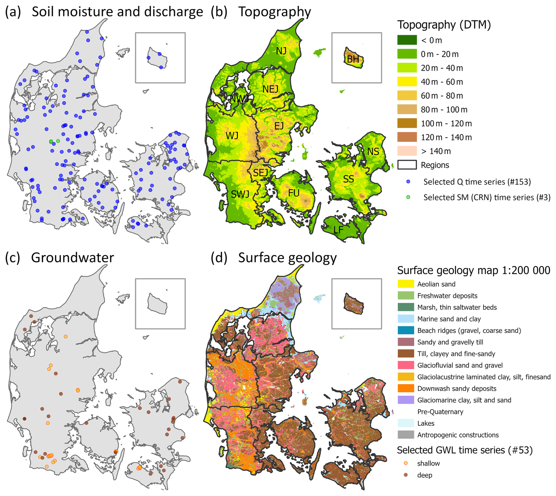
Figure 1 (a) Selected soil moisture and streamflow stations and (c) selected groundwater wells for drought analysis (shallow wells with filter depth < = 10 m, deep with filter depth > 10 m). (b) Topography of Denmark, with regions outlined in black. (d) Surface geology map of Denmark.

2.3.2 Streamflow data

Streamflow data in Denmark has been monitored relatively consistently over the last decades (Overfladevandsdatabasen, https://odaforalle.au.dk/main.aspx, last access: 18 June 2026) and data are generally of high quality, with few gaps. The entire dataset of streamflow stations in Denmark in the period 1990–2023 consists of 579 stations measuring daily streamflow. The selection of stations for validating the drought indices is based on a previous quality assurance effort when selecting streamflow stations for the calibration of the DK-model (Stisen et al., 2019). This quality assurance focused on stations with a catchment area above 15 km², as both measurement and model error increases for very small catchments, and where streamflow was unaffected by factors such as pumping stations or sluices, and had a data coverage of at least 98 % of all days in the period. This resulted in a total of 153 stations for the validation analysis (Fig. 1). The selection criteria for streamflow stations are higher than for groundwater levels and soil moisture simply because data are abundant and multiple long time series with good national coverage exist.

2.3.3 Soil moisture data

Due to the DK-model's resolution of 500 m grid scale, it is unsuitable to evaluate its performance using conventional soil moisture measurements, which typically represent small soil areas or volumes at the centimetre scale and exhibit large variability at small scales (Famiglietti et al., 2008; Zignol et al., 2025). We only use large-scale soil moisture measurements in the model validation. Unfortunately, large-scale soil moisture measurements are generally rare. There are only five sites across Denmark with such measurements, all applying the cosmic ray method (CRN); two have just 1 to 2 years of data, while the other three have measurements for around 10 years (Jensen and Refsgaard, 2018). Only the three longest datasets could be included in the evaluation (Fig. 1). The CRN method is based on the inverse relationship between neutron intensity from cosmic radiation and the water content (hydrogen) in the soil (Andreasen et al., 2017). The CRN sensors provide soil moisture within the root zone as measurement depth is integrated non-linearly from the soil surface to around 10–75 cm depth in the soil column, depending on water content (Zreda et al., 2012). The stations have a horizontal footprint of 200–300 m, comparable to the grid size of the hydrological model (Andreasen et al., 2017).

2.4 Drought indices

A multitude of different drought indices exist and are described in the literature (see e.g., Zargar et al., 2011). They often cover different parts of the hydrological cycle, and thus, represent different variables, e.g., precipitation or streamflow. Often, they are either threshold-based or standardized (de Matos Brandão Raposo et al., 2023), meaning that they are either based on drought definitions characterized by crossing a certain threshold (e.g., a percentile of streamflow), or deviations of a time series from its normal (e.g., more than two standard deviations from the mean). Newer emerging indices are, for example, based on combining existing indices into composite ones (Raible et al., 2017) or indices modified for specific conditions, e.g., ephemeral streams (Aon and Biswas, 2024). Indices can be calculated from various observations of the hydrological cycle (Haas and Birk, 2017), remote sensing products or land surface models (Gaona et al., 2022), as well as hydrological models (Sutanto et al., 2024) or a combination of the above.

Generally, it is recommended to use standardised indices when comparing drought signals across different regions and compartments of the hydrological cycle (de Matos Brandão Raposo et al., 2023; Teutschbein et al., 2022; World Meteorological Organization (WMO), 2012). Due to the differences in precipitation regime from east to west in Denmark (Stisen et al., 2012), standardised indices were also chosen in this study. An overview of the indices used in this study is given in Table 1.

Table 1 Overview of drought indices used in this study.

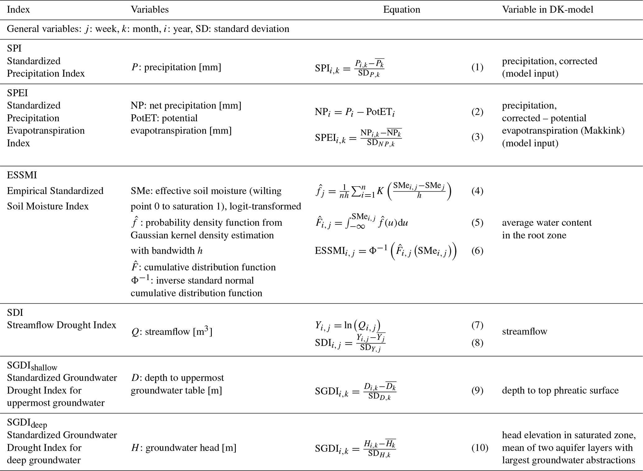
For the meteorological drought signal, we applied the commonly used SPI (Standardized Precipitation Index) (McKee et al., 1993) for precipitation, and the SPEI (Standardized Precipitation Evapotranspiration Index) for net precipitation (Vicente-Serrano et al., 2010), Eqs. (1) to (3), which we refer to as meteorological drought indices. The other indices, covering different compartments of the hydrological cycle, are referred to as hydrological indices. For soil moisture, we applied the ESSMI (Empirical Standardized Soil Moisture Index) (Carrão et al., 2016), Eqs. (4) to (6), as it allows for robust handling of bounds such as full saturation commonly occurring in simulated soil moisture values. For streamflow we use the SDI (Streamflow Drought Index) (Nalbantis and Tsakiris, 2009) with log-transformed streamflow values, Eqs. (7) and (8), as it is a common index in the literature (Gonçalves et al., 2023; Kim et al., 2024; Zhong et al., 2020), and its formulation originates from the SPI. This is also the case for the groundwater index used in the study, the SGDI (Standardized Groundwater Drought Index) (Bhuiyan et al., 2006; Bloomfield and Marchant, 2013), Eqs. (9) and (10). Examples of SGDI in the literature include Han et al. (2019), Ling et al. (2024), and Zhu et al. (2023).

Common for the standardized indices we used (Table 1) is that they indicate the deviation of the current status of, for example, groundwater levels, from the typical seasonal cycle, as defined by the mean monthly or weekly climatology over the reference period. For all indices, values below 0 correspond to below-average or dry conditions. Furthermore, the resulting index values are translated to categories of drought as established by McKee et al. (1993) and commonly used since: the different categories are “moderate drought” (−1 to −1.5), “severe drought” (−1.5 to −2), and “extreme drought” (below −2).

2.4.1 Drought indices based on observational time series and DK-model simulations

For the calculation of drought indices, a 30-year reference period from 1991 to 2020 was chosen. As noted in Table 1, SPI and SPEI are calculated based on monthly values and climatologies, as most commonly practiced and recommended (World Meteorological Organization (WMO), 2012). Similarly, the SGDI is calculated based on monthly values. In principle, SGDI could also be calculated at a higher frequency, but the scarce observation frequency limits us to using monthly values. Soil moisture indices are often calculated at higher frequency (Narasimhan and Srinivasan, 2005), and we calculate the ESSMI weekly to account for short-term changes (e.g. spring vegetation development). Similarly, to allow better representation of seasonal development of these quickly reacting variables and due to good data availability, we calculate the SDI weekly. Both ESSMI and SDI are resampled from weekly to monthly values in the result sections.

Calculation of the SPI and SPEI starts with fitting a suitable distribution function to the observed climatologies (Lloyd-Hughes and Saunders, 2002; McKee et al., 1993). Often, especially in climates with more intermittent precipitation, a gamma distribution is chosen. However, for our case of Denmark, a Shapiro–Wilk normality test revealed that the distribution of monthly climatology precipitation grid values can be fitted by a normal distribution: the normality hypothesis only had to be rejected for 14.9 % of grids and months (p < 0.01). Preliminary tests revealed that other distributions, such as gamma distributions, could also be fitted; however, not more successfully than the normal distribution, and fitting sometimes was unstable, yielding implausible extreme values. This might also be related to the relatively short reference period of 30 years. Hence, we preferred the simple assumption of normal distribution. The SGDI in its original form uses a normal score transformation based on empirical values, as groundwater level time series can exhibit a variety of different distributions (Bloomfield and Marchant, 2013). However, for the sake of simplicity (across indices) and the possibility of extrapolation (e.g. to future climate), we opted for a parametric normal distribution fitting like for SPI and SPEI. For groundwater, normality had to be rejected for 7.8 % (shallow) and 19.9 % (deep groundwater) of grids and months. Similarly, streamflow normality had to be rejected for only 3.4 % of grids and weeks. Simulated soil moisture values, however, stand in contrast to that, as they are bound by saturation (and, less important in Danish conditions, residual water content). For a significant number of grids and timesteps, values are constant at e.g. the saturation content, hindering distribution fitting. Hence, we chose the ESSMI relying on the empirical distribution, and using a kernel density estimate to obtain a smooth approximation that permits limited extrapolation beyond the observed data.

Drought indices were calculated based on the observational datasets introduced in Sect. 2.3, referred to as obs in the following, as well as the simulation results from the DK-model introduced in Sect. 2.1, referred to as sim in the following. Sim indices are calculated for every grid or roughly every 500 m along the streams (referred to as q-points) of the DK-model based on the model outputs indicated in Table 1. The continuous simulations allow abstraction of drought indices for the entire period between 1990 to 2023, relative to the reference period 1991 to 2020. Obs indices are calculated for every streamflow station, groundwater well, and CRN soil moisture station in the quality-assured dataset. Where data coverage allowed, the full reference period 1991 to 2020 was used. However, many observational time series had limited coverage; here, the reference period was shortened accordingly, down to 10 years of the soil moisture observations. To allow a direct evaluation of the DK-model's ability to reproduce drought signals – and more generally signals of meteorological anomalies – in the hydrological cycle, drought indices from the DK-model results were calculated separately for each of the observation locations, i.e. each specific matching grid or streamflow point in the DK-model output. Those indices are referred to as sim@obs and were calculated based on simulated time series reduced to the same data availability as the respective observation data. This allows a direct, unbiased comparison of obs and sim@obs indices based on matching locations and reference periods.

2.4.2 Drought propagation and lag

To evaluate the propagation of meteorological drought and anomalies in general through the hydrological cycle, SPI and SPEI were calculated not only for monthly values (1-month SPI and SPEI), but also for different accumulation periods ranging from 2 to 60 months (2-month to 60-month SPI and SPEI, referred to as SPI_acc2 etc.). For example for the 3-month SPI, the index value for March of a specific year is calculated based on the total precipitation of the 3 months January to March of the same year, relative to the normal total precipitation for January to March across all years of the reference period. Different compartments of the hydrological cycle are expected to be sensitive to different accumulation periods of precipitation, generally moving from faster-reacting soil moisture and streamflow to slower-reacting shallow and deep groundwater. The accumulation periods were determined by calculating correlations between each of the hydrological index time series and SPI_acc or SPEI_ac in the same grid or q-point, respectively, finding the accumulation period with the highest correlation. The performance of the DK-model is tested by comparing this accumulation period signal in the model (sim@obs) in relation to the signal found using the observations (obs). This is to test if the modelling system correctly represents the connections and propagation in the different natural systems.

Moreover, it was investigated how well drought and anomaly propagation to groundwater can be informed by more simple controlling variables than a hydrological model. Such controlling variables can be related to local geology, or the depths to the aquifer or groundwater table, local groundwater gradients, etc. Some of these potentially controlling variables (see e.g., Bloomfield and Marchant, 2013; Li and Rodell, 2015; Schuler et al., 2022) can be directly derived from the geological setting, in our case from the national well database Jupiter. Others require a hydrological model or some knowledge of groundwater dynamics. Here we focus on hydrological-model-independent variables derived from the well database:

• filter depth,

• observed groundwater depth,

• overburden (the total thickness of material above the well's aquifer),

• accumulated clay thickness (as overburden, but only accumulating clayey material),

• the number of shifts between clay and sand layers (as an expression of geological complexity).

The latter two variables are included because the Danish Quaternary deposits, in which most of our wells are placed, generally can be simplified to a series of alternating clay and sand layers. These five variables were extracted for the 53 groundwater wells. Then, across the groundwater wells, correlations between these variables and the wells' observed drought lags were determined, as well as multi-variable linear regression model tested, and compared to DK-model results. This allowed to an evaluation whether the DK-model outperforms simple statistical methods in terms of drought and anomaly propagation in the groundwater.

2.4.3 Evaluation of observational and simulated indices

The performance of the indices, that is the agreement between drought indices based on observed and simulated variables, is evaluated using complementary metrics that asses both continuous signal agreement and discrete drought detection skill across the entire available time series. Continuous signal agreement is evaluated using the Pearson correlation coefficient (r), the mean absolute error (MAE), and the root mean square error (RMSE) between observed and simulated indices, which sheds light on temporal coherence and magnitude differences of standardized anomalies. The evaluation is performed three-fold:

• i.

  On individual time series: for all the selected observational time series of soil moisture, streamflow, and groundwater, every index time series (obs) is evaluated against the corresponding simulated time series (sim@obs).

• ii.

  On individual time series: for all the selected observational time series of soil moisture, streamflow, and groundwater, the accumulation period correlation to SPI (SPEI) for the index time series (obs) is evaluated against the corresponding signal in the simulated time series (sim@obs).

• iii.

  Across Denmark: for every index, an aggregated drought index time series as average across Denmark is calculated for all observations (obs) and compared with the corresponding aggregated drought index series based on the simulations (sim@obs). Furthermore, the corresponding aggregated simulated drought indices (sim@obs) are also compared to the overall Denmark-wide drought index series (sim), to evaluate the spatial representativeness of the observation points of the entirety of Denmark.

In addition, drought detection skill is assessed using the F1 score, which evaluates the model's ability to correctly identify threshold-defined drought events. For this purpose, standardized drought indices are transformed into binary drought occurrence time series based on thresholds for moderate (< = −1), severe (< = −1.5), and extreme (< = −2) droughts. At each time step (month), sim and obs drought occurrence are classified as true positive, false negative, false positive or true negative, and the F1 score is computed as the harmonic mean of precision and recall of detection; see Eq. (11).

$$\begin{array}{}\text{(11)}& \text{F1}=\mathrm{2}\cdot {\displaystyle \frac{\text{precision}\cdot \text{recall}}{\text{precision}+\text{recall}}}\end{array}$$

with

$$\begin{array}{}\text{(12)}& \text{precision}={\displaystyle \frac{\text{TP}}{\text{TP}+\text{FP}}},\text{recall}={\displaystyle \frac{\text{TP}}{\text{TP}+\text{FN}}}\end{array}$$

The drought detection F1 scores are calculated on individual time series (point (i) in the list above) as well as across Denmark for aggregated time series (iii).

3 Results

3.1 General DK-model performance

Figure 2 sums up the overall DK-model performance, showing cumulative distributions across the multiple conventional (i.e. not drought-related) calibration targets. Across 305 streamflow stations, a median KGE of 0.67 is reached, and the overall water balance error Fbal is 0.01, with a mean absolute error of 0.15. Fbal is calculated as (Q_obs − $Q_{\mathrm{sim}})/Q_{\mathrm{obs}}$. Across the 153 selected streamflow stations for the further drought analysis with long time series, performance is slightly better with a median KGE of 0.70, an overall water balance error of 0.02 and a mean absolute error of 0.14. In terms of groundwater performance, the mean absolute error across 39 514 wells with groundwater level observations is 3.67 m, with a mean error of 0.47 m. For the 53 selected wells for drought analysis, these errors are reduced to a RMSE of 2.37 m with a mean error of 0.46 m; which likely reflects their higher quality measurements. All mean errors are provided as obs − sim. Seasonal groundwater level amplitudes are reproduced with a mean absolute error of 0.65 m across 400 groundwater level time series with sufficient data to calculate average seasonal amplitudes. Across the 53 selected wells, the amplitude mean absolute error is 0.60 m. Observed amplitudes are 1.06 m on average, and mean absolute errors are skewed by outliers; the median absolute error is 0.41 m. Lastly, the drain fraction (average simulated drain flow per grid cell relative to precipitation) was included in the calibration: artificial drainage represents an important hydrological process in Denmark, with significant spatial variation, which is often overlooked. Hence, a Machine Learning generated map of drain fraction was used as a target (Schneider et al., 2025); panel (e) in Fig. 2 shows the residuals of the model against that map, indicating that the DK-model slightly underestimates the amount of artificial drainage. DK-model performance during validation periods 1990 to 1999 and 2011 to 2019 closely matches performance in the calibration period 2000 to 2010 reported here; see Fig. B1 in Appendix B.

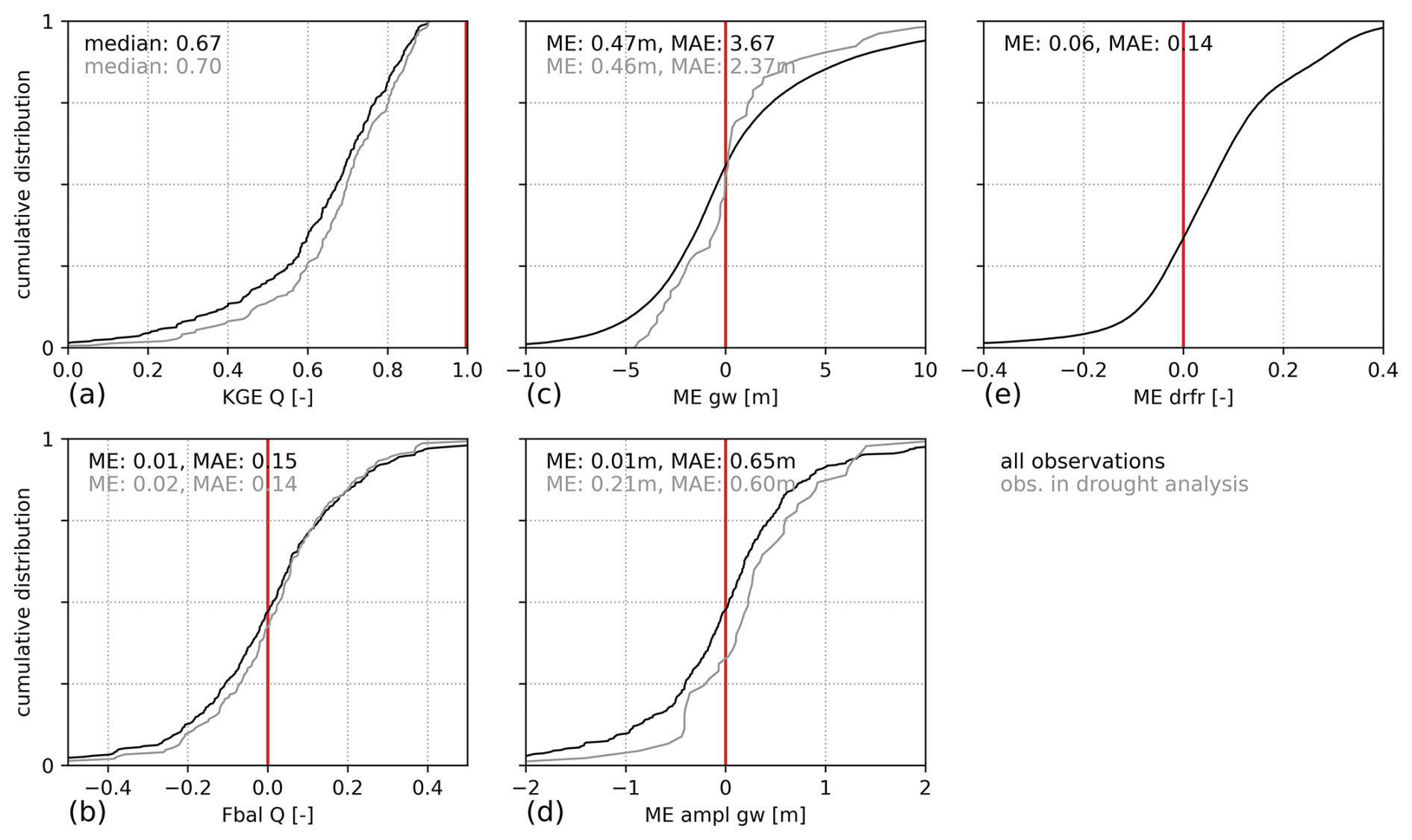
Figure 2 DK-model calibration period performance. (a) KGE [–] and (b) water balance error [–] for 305 stream flow stations. (c) Residuals against groundwater level measurements in 39 514 wells. (d) Residuals against seasonal groundwater level amplitudes in 400 wells. (e) Residual against ML predictions of drain fraction. The 153 selected streamflow stations as well as 53 selected groundwater wells for the drought analysis are indicated with grey in panels (a) and (b), and (c) and (d), respectively. Optimal values marked with red.

3.2 Evaluation of drought index time series: observations vs. DK-model simulations

Each of the individual observation time series of indices (obs) is compared to the simulated values at the respective locations (sim@obs). This is done based on monthly statistics for all drought indices, also those that originally were calculated on a weekly basis (SDI, ESSMI). To give the reader an impression of the time series, examples at observation points for the four drought indices are shown in Fig. 3, including the Pearson correlation coefficient r and the RMSE between the obs and sim@obs indices time series. The examples were chosen to be somewhat representative of overall performance (compare Fig. 4).

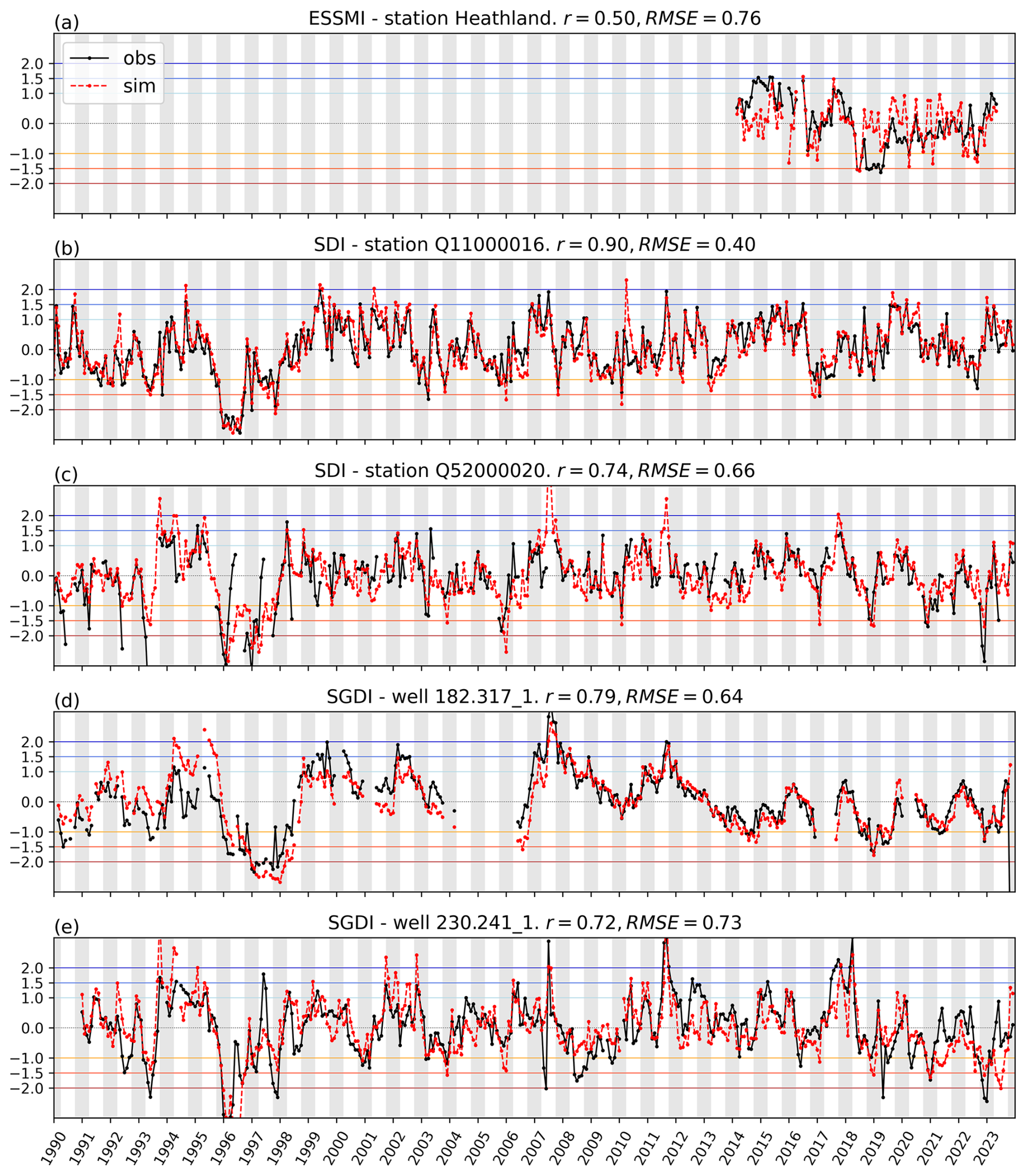
Figure 3 Examples of observed drought indices (black), compared to simulated values (red) at example CRN stations (a), streamflow stations (b, c) or wells (d, e). Winter periods (October to March) with grey background. Thresholds for moderate, severe, and extreme droughts (and wet conditions) are marked with horizontal lines.

Figure 4 shows the correlation coefficients between obs and sim@obs across all observation points for each of the four indices. In panel (a), those values are shown on a map of Denmark. In panel (b), the cumulative distribution of the correlation coefficients is shown both for the entire time series, and separately for dry periods only (defined by a obs index < 0). Generally, performance is highest for the SDI, followed by SGDI and lastly ESSMI. Performance is slightly better in the western parts of the country. It can also be seen that the correlation coefficient r tends to be lower during dry anomaly periods. However, this does not necessarily reflect lower performance; rather it is related to the sensitivity of Pearson's r to the range of occurring values, which is restricted to roughly half if only looking at dry periods. This is also confirmed in Table 2, which shows the median values of correlation coefficients across all time series. Values are provided across the entire period, and separately for dry and wet periods, which are defined by negative and positive obs index values, respectively. Here, r decreases for both wet and dry periods compared to the full series, which is expected because truncating the distribution reduces variance and covariance, which mathematically leads to smaller Pearson correlation coefficients. Thus it is not necessarily indicative of a poorer performance of the model in dry or wet conditions.

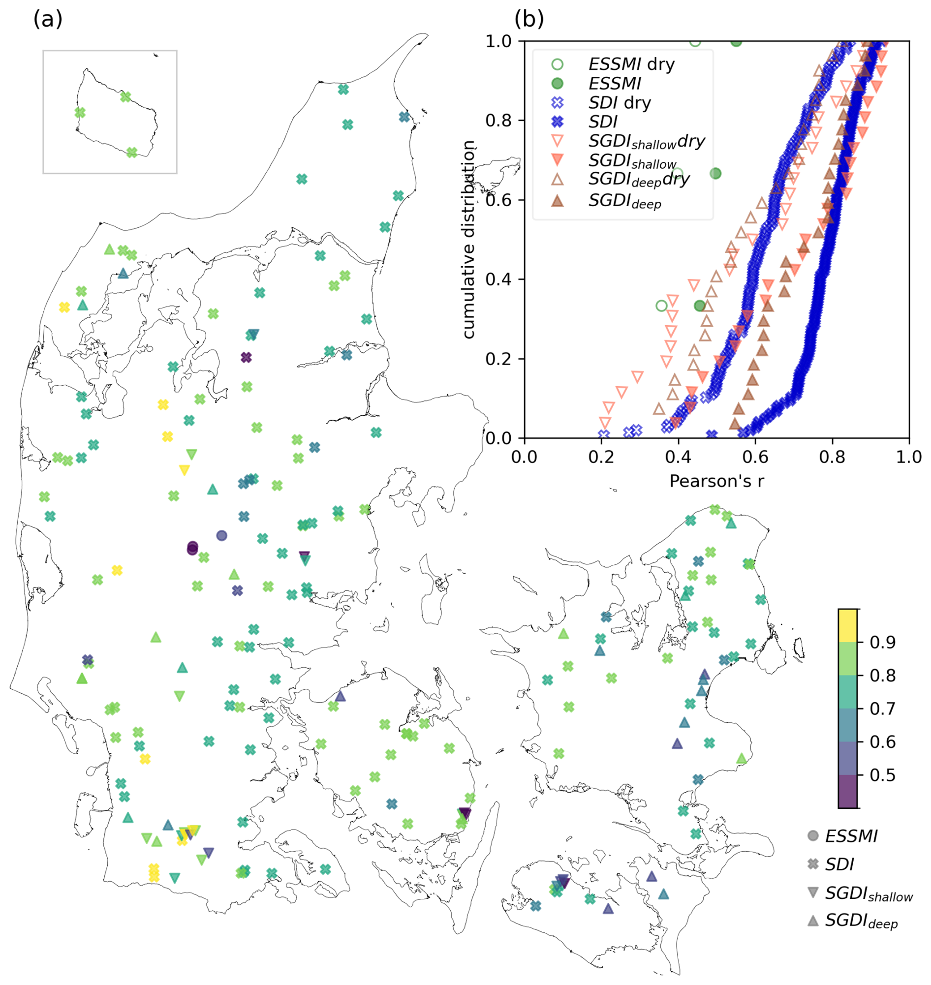
Figure 4 Performance of the simulated hydrological drought indices (Pearson's r) for the observed points. Panel (a) shows performance in every observation point across the entire period, with colours indicating r values and marker types indicating observation types. Panel (b) summarizes the performance distribution. Here, r values are shown separately for the entire period and dry periods (observed index < 0).

Table 2 Overview of correlation performance of drought indices for Denmark. Time series median: median of performance of the individual observed time series. DK statistics: obs vs. sim@obs: aggregated observed vs. aggregated simulated time series at points of observations. obs vs. sim: Aggregated observed vs. aggregated simulated time series across all of Denmark. sim@obs vs. sim: Aggregated simulated time series at points of observations vs. across all of Denmark. Numbers in parentheses indicate values for dry and wet (in italic) periods separately.

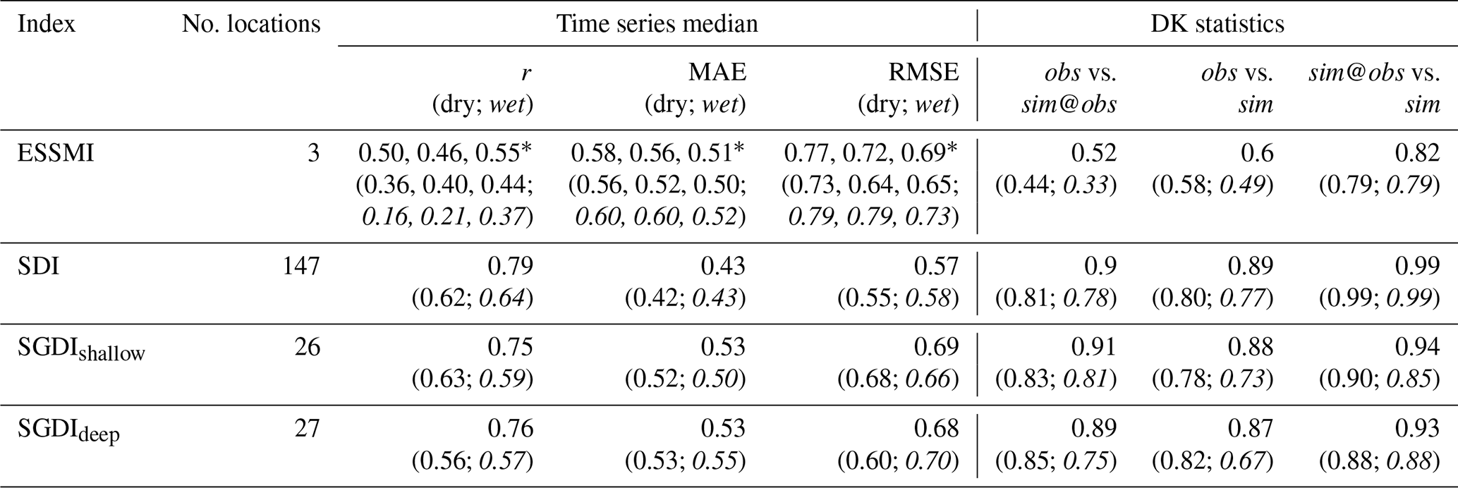
^* Statistics for all three stations are reported here, in order Harrild, Voulund, Gludsted.

Table 2 summarizes the correlation coefficients to median values across all time series for each of the four indices. Values are provided across the entire period, and separate for dry and wet periods, defined by negative and positive obs index values, respectively. In the “DK statistics” columns of Table 2, we also include correlation coefficients between aggregated drought index time series aggregated all observation locations (obs, sim@obs) or across all of the DK-model domain (sim). The overall performance at the individual time series level is at median Pearson's r values above 0.75 across all conditions, and values around 0.6 during dry periods only. The only exception to this is the ESSMI with lower r values mostly between 0.4 and 0.5. When looking at aggregated values across all of Denmark (DK statistics), the performance is better with r values close to or above 0.9 for SDI, SGDI_shallow and SGDI_deep. Again, the only exception is ESSMI which has lower correlations.

Table 3 summarizes the drought detection performance. This is done for three drought categories: Moderate drought, with drought index values below −1, severe drought with values below −1.5, and extreme drought for values below −2, all based on monthly values of sim and obs indices. The agreement in detection of those drought events then is provided as F1 scores, where performance is moderate to good. Exceptions are extreme droughts – which partly owes the fact that they are rare events badly defined by the observed and simulated data, occurring theoretically only during 0.75 times during a 30-year climatology. Also, as before, soil moisture drought performance is deteriorated compared to the rest. Drought detection performance was also evaluated for time series aggregated across all of Denmark (DK statistics), where agreement is better with F1 scores mostly around 0.7 or 0.8. The exception is soil moisture drought.

Table 3 Overview of drought detection performance for Denmark. F1 scores are provided as the median of the individual time series.

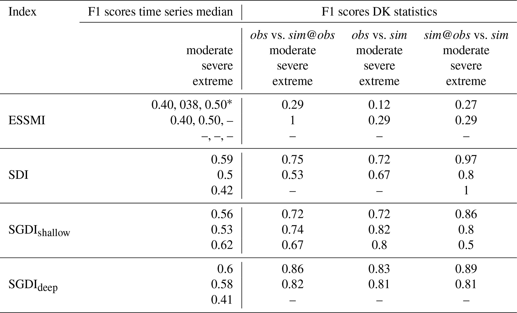
^* Statistics for all three stations are reported here, in order Harrild, Voulund, Gludsted.

3.3 Accumulation period performance

The SPI was calculated for different accumulation periods from 1 to 60 months, resulting in 60 time series from SPI_acc1 to SPI_acc60. For each of these time series, a correlation to the hydrological drought index was calculated. The accumulation period of the SPI that exhibits the highest correlation to the hydrological drought index indicates the dynamics of anomaly propagation from a precipitation anomaly to a hydrological impact. This is done separately for the obs and sim@obs index time series for ESSMI, SDI, and SGDI, and the resulting optimal SPI accumulation periods can be compared. If the model captures the development time and interconnectivity of the syst emsatisfactorily, the optimal SPI accumulation time for obs and sim@obs should be similar.

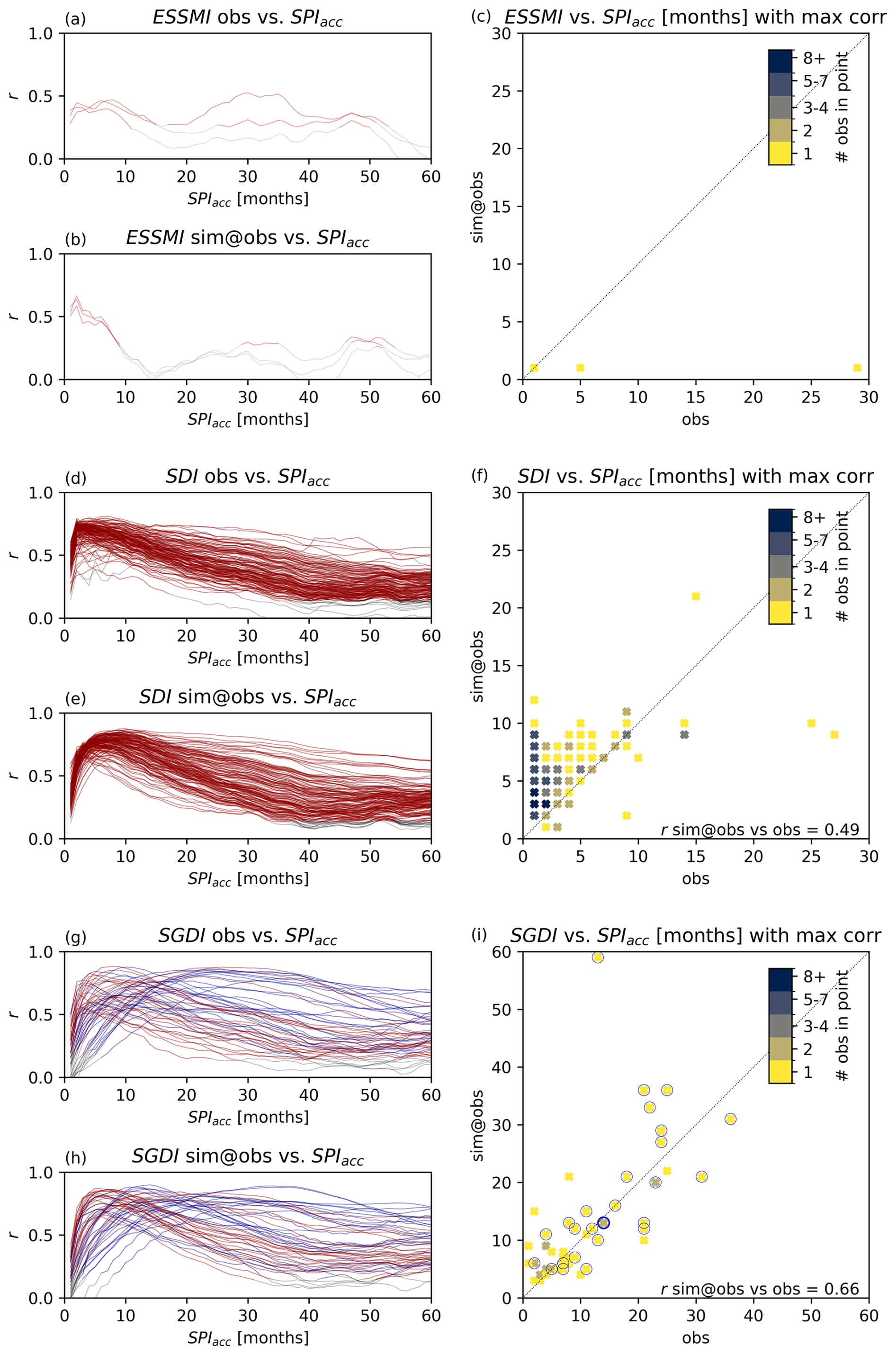
Figure 5 Left column: correlation coefficients of SPI accumulation periods against observed and simulated time series of ESSMI (a, b), SDI (d, e), and SGDI (g, h), respectively. Significant correlations (p < 0.01) in red (or blue for wells representing SGDI_deep), remaining in grey. Right column: scatter plots of optimal accumulation period of SPI for correlation to ESSMI at the 3 CRN stations (c), SDI at the 153 streamflow stations (f), and SGDI at the 53 groundwater wells (i), where wells representing SGDI_deep are marked with blue outlines (two wells in same point: thick blue outline). Optimal SPI accumulation period for simulated time series along the y axis, and for observed time series along the x axis.

Figure 5 shows the results of this analysis. For each of the individual observation points, all 60 accumulation periods from 1 to 60 months for SPI_acc were tested. The resulting correlation coefficients are shown in the plots in the left column, separately for each of the obs and sim@obs time series. The SPI accumulation period yielding the highest correlation for obs and sim@obs, respectively (i.e. the peak of each curve in the left column plots), is then shown in scatter plots against each other in the right column, to evaluate whether obs and sim@obs indices reflect similar accumulation periods.

For streamflow (SDI), the DK-model tends to delay drought propagation more than seen in observations: the majority of obs indices (86 of 153 stations) show the highest correlation of SDI to SPI_acc1 or SPI_acc2, whereas sim@obs indices are correlated to accumulation periods of up to 10 months. However, it has to be noted that the optimal accumulation periods do not seem to be well defined; see especially the obs indices, which correlations only slowly decay up to roughly SPI_acc10. For groundwater (SGDI), the time series seem to be more grouped, with some having short accumulation time correlations (up to 6 months), others longer (7 to 12 months), and some very long (above 12 months). For the obs indices, roughly one third of the 53 wells fall in each of these categories: 19 with up to 6 months, 15 with 7 to 12 months, and 19 with above 12 months. The distribution for sim@obs indices is very similar, with 18, 15, and 20 wells in the respective groups. Also, the typically longer observed accumulation periods for SGDI_deep are reproduced in sim@obs indices. Again, ESSMI is the exception with the sim@obs indices having the highest correlation to SPI_acc2, whereas the obs indices exhibit high correlations for SPI_acc6 to SPI_acc8, but also around 30 months.

From the scatter plots, it can be confirmed that for SDI and SGDI, the optimal SPI accumulation periods broadly agree, with correlation coefficients between the optimal accumulation periods of obs and sim@obs of 0.49 and 0.66, respectively. This indicates that the DK-model can capture the major dynamics of drought propagation through the hydrological cycle, especially in the groundwater. The soil moisture performance is poorer, but the evaluation is also restricted by the limited amount of data.

The different accumulation periods across the observations suggest there are regional differences in the response time to precipitation. Figure 6 shows the accumulation period of SPI which yields the highest correlation to each of the sim indices, mapped for all of Denmark in the top row. The bottom row shows what the highest correlation is (between sim index and SPI_acc with the optimal accumulation period). Those correlations are generally high, with Pearson's r values mostly above 0.5, for SDI and SGDI often even above 0.75.

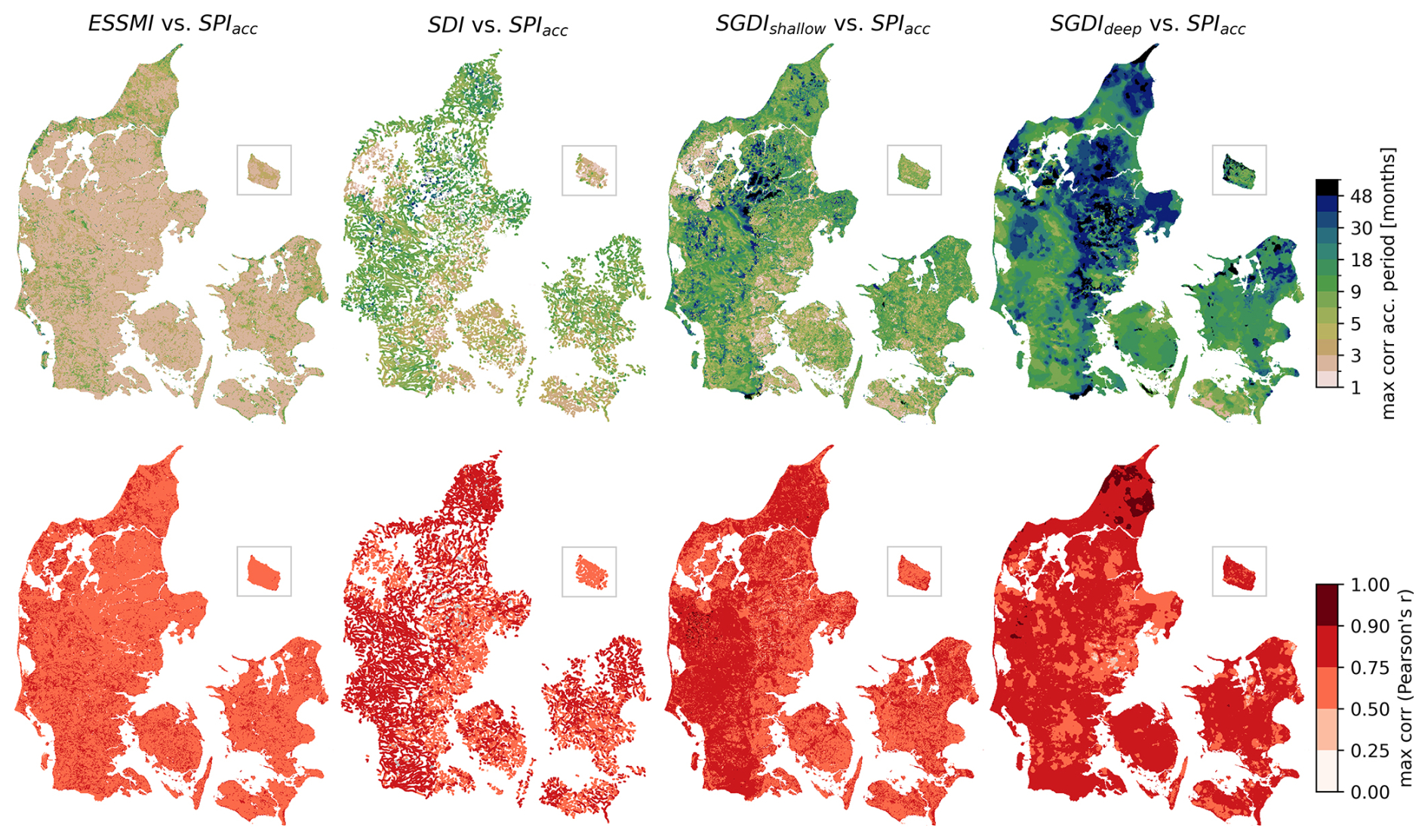
Figure 6 Top row: accumulation period of SPI_acc yielding maximum correlation with the hydrological drought index per DK-model q-point or grid. Bottom row: maximum correlation between the hydrologic drought index and SPI_acc of the respective accumulation period. Non-significant correlations (p > 0.01) are masked grey (e.g. isolated areas for SDI and SGDI_deep in eastern Jutland).

Note that the drought propagation from SPI to hydrological drought is very similar to the drought propagation from SPEI to hydrological drought. To maintain clarity, we focused on propagation from SPI here; corresponding versions of Figs. 5 and 6 for SPEI can be found in Appendix C, Figs. C1 to C4.

The skill of the DK-model to reproduce observed propagation expressed as accumulation periods of SPI was also evaluated by comparing it against correlations and simple linear regression models between geology-derived controlling variables and the optimal SPI accumulation periods. Table 4 summarizes the results, showing correlations between the controlling variables and the SGDI lag (SPI_acc to SGDI_shallow and SGDI_deep), separate for shallow and deep wells as well as combined across all 53 wells.

Table 4 Correlation between well geologic variables and their experienced lag expressed as the SPI accumulation periods with the highest correlation to observed SGDI (compare Fig. 5). Values are provided as Pearson's r and Kendall's tau, separately for shallow wells, deep wells, and all wells. Last row: correlation between the drought lags based on observed and simulated SGDI. Best performance across each column marked bold. Non-significant (p > 0.01) correlations in (brackets).

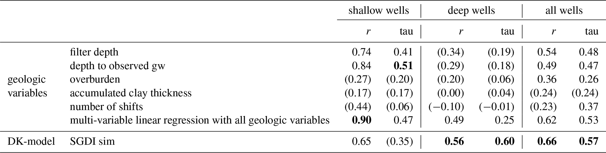
The correlation between the individual geological variables and SGDI lag is larger for shallow wells than for deep wells. Significant correlations, however, can only be found for filter depth and depth to observed groundwater table for the shallow wells and across all wells, and for overburden across all wells. No significant correlations exist for the deep wells. The DK-model simulated SGDI lag, conversely, shows significant correlation for all well groups, and demonstrates the highest predictive ability across deep wells and across all wells. The DK-model also outperforms a multi-variable linear regression model based on the five geological variables. Only for the shallow wells, single geological variables such as the depth to the observed groundwater table or the multi-variable linear regression model show better correlations to the SGDI lag than the DK-model.

3.4 Drought performance across Denmark

In the “DK statistics” columns of Table 2, we include correlation coefficients between the combined drought index time series aggregated across all observation locations (obs), the same type of combined index for simulation time series (sim@obs), and one combined from the entire DK-model domain (sim). This sheds light on different aspects. First, the performance of the DK-model in simulating observed drought indices (obs vs. sim@obs), on an aggregated level. Here, the performance is even better than for individual time series, with r values close to or above 0.9 for SDI, SGDI_shallow, and SGDI_deep. Again, the only exception is ESSMI, which is not as well correlated.

Secondly, we can evaluate the performance of the observations concerning the entire domain (obs vs. sim), which proves very similar to the performance when comparing to simulations from the actual locations of the observed time series (sim@obs). Similarly, the index calculated for simulation data at observation points is very strongly correlated to the behaviour of the entire domain (sim@obs vs. sim).

Aggregated drought indices across all of Denmark, as monthly means for the years 1990 to 2023, are shown in Fig. 7. Generally, drought patterns between obs and sim@obs indices agree well, as already indicated by good correlation performance values reported in Table 2 above. Notably, there is also good agreement between the indices based on the relatively few observation points (obs and sim@obs) and the simulated Denmark-wide drought index dynamics (sim) across all grids or streamflow points in the DK-model. Thus, the observation points are thought to be representative of the behaviour of the entire domain and can therefore be used to evaluate the general DK-model drought performance.

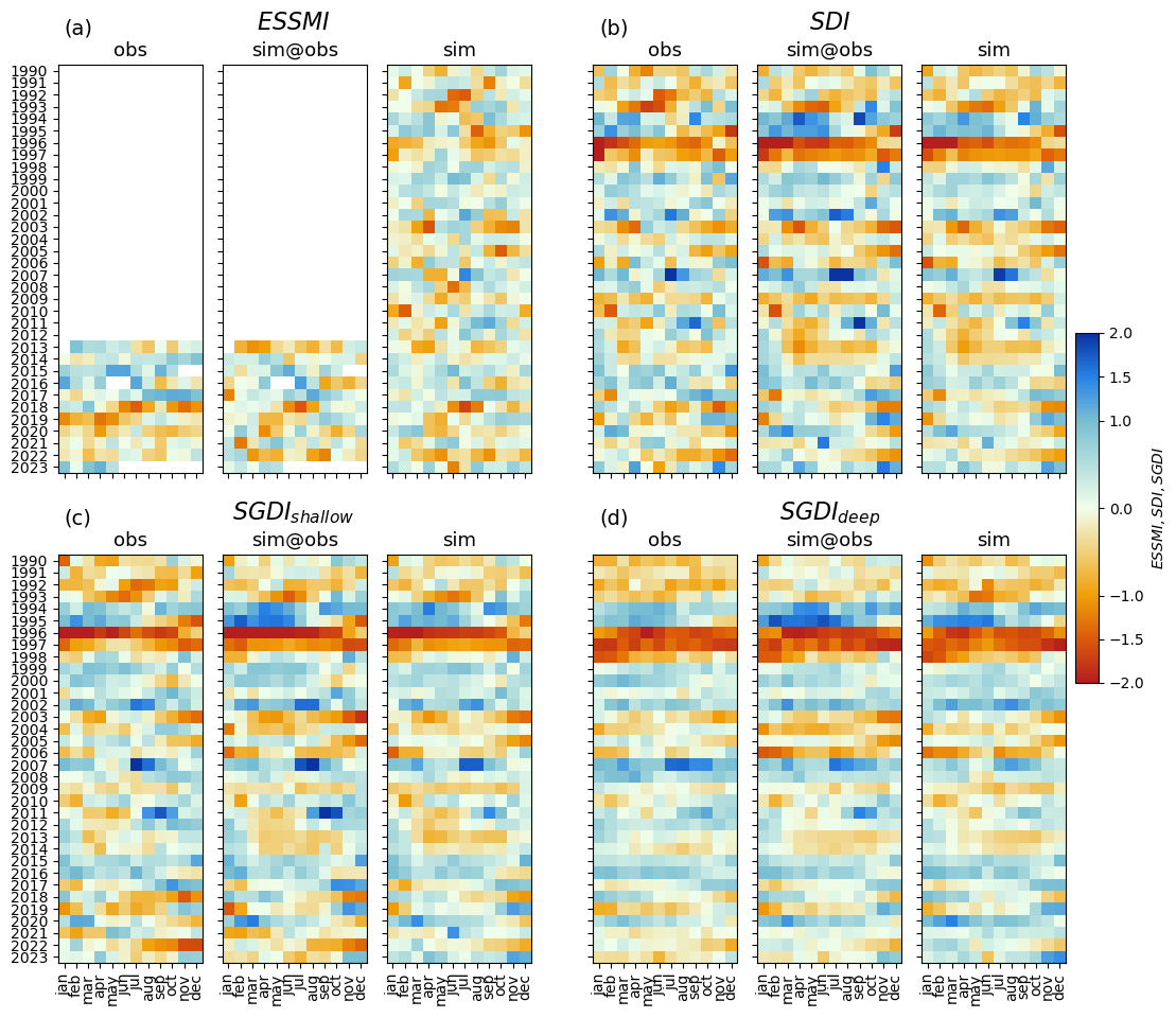
Figure 7 Mean monthly drought indices for ESSMI (a), SDI (b), SGDI_shallow (c) and SGDI_deep (d). Each panel shows from left to right: mean obs drought indices, mean sim@obs drought indices, mean sim drought indices across all of Denmark.

Figure 8, top row, shows mean monthly drought indices for all of Denmark. Monthly SPI and SPEI values show little autocorrelation in time, and soil moisture anomalies (ESSMI) closely follow the anomalies in (net) precipitation. Effects of meteorological drought keep accumulating, though, when moving further through the hydrological cycle: SDI starts showing more continuous, more extended drought periods (or wet anomalies), and SGDI_shallow and SGDI_deep react with even more delay, exhibiting longer continuous drought periods in line with results shown in Figs. 5 and 6. The middle and bottom row then show the differences between two regions in Denmark, western Jutland and eastern Jutland (WJ and EJ in Fig. 2b), which are dominated by more sandy and clayey soils, respectively. In the more sandy western Jutland, drought signals propagate faster from meteorological to hydrological drought, especially visible in the deep groundwater (SGDI_deep). The more clayey eastern Jutland experiences slower drought propagation, particularly to the deep groundwater, as evidenced for example by a delay of few months in both the onset of and recovery from the SGDI_deep drought in 1996/97 compared to West Jutland.

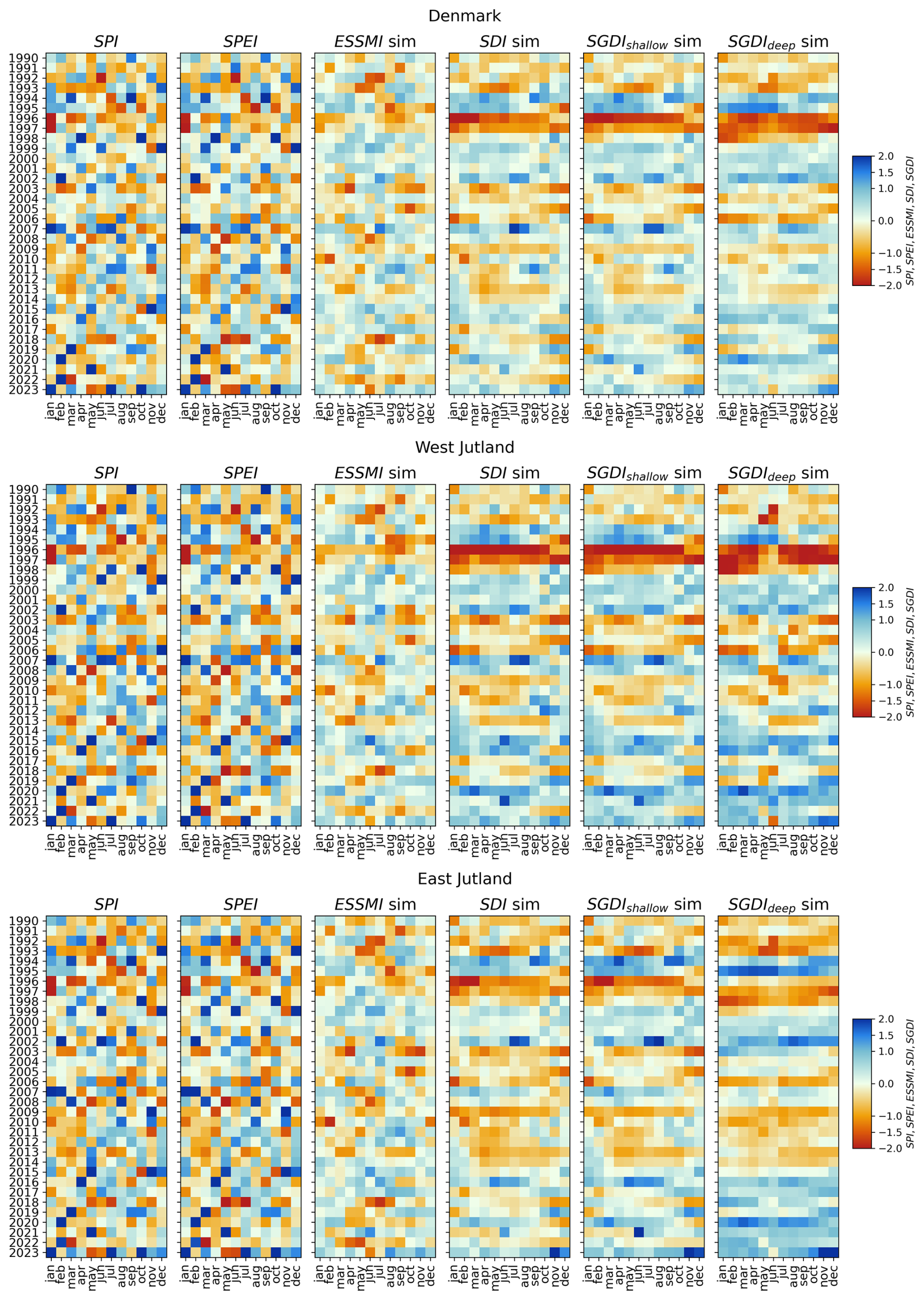
Figure 8 SPI, SPEI and sim drought indices across all of Denmark (top), western Jutland (middle) dominated by sandy soils, and eastern Jutland (bottom) dominated by clayey soils.

Figure 9 shows maps of drought indices for all of Denmark for May 2020, and illustrates diverging response times of the different hydrological compartments. The first column shows SPI_acc2 and SPI_acc12, whereas the remaining maps show the four sim indices. The month of May 2020 is characterized by a soil moisture drought, with ESSMI values below −1 (moderate drought) in large parts of the country and partly below −1.5 (severe drought). Soil moisture is low as May and April 2020 had been experiencing unusually low precipitation amounts, reflected in SPI_acc2 values being mostly below normal values. The remainder of the hydrological cycle, however, remains in normal to wet conditions, as expressed by SDI, SGDI_shallow, and SGDI_deep. This is due to their slower response to precipitation anomalies than fast-reacting soil moisture (compare Figs. 5 and 6), and the wet preceding conditions in the entire 12-month period prior to May 2020, as expressed by high (i.e. wet) SPI_acc12 values.

Figure 9 Sim drought indices from the DK-model for the example of May 2020, together with SPI_acc2 and SPI_acc12.

3.5 Groundwater sensitivity to summer and winter droughts

For Danish conditions with winter being the main recharge season, meteorological droughts during the winter season have a comparably larger effect on groundwater drought development. This is illustrated in Fig. 10, where the 34 years 1990 to 2023 are separated into two seasons, the winter half-year October to March and the summer half-year April to September. Then, they are further split into their meteorological drought condition across each winter or summer, defined by the SPI_acc6 at the end of the respective 6-month period being below −0.5 (drought) or above 0.5 (non-drought), resulting in 11 drought winters and 10 non-drought winters, as well as 12 drought summers and 10 non-drought summers. Figure 10 then shows the developments of the SGDI_deep values throughout each of the drought or non-drought winters or summers, relative to the SGDI_deep value at the start of each season. The simulated sensitivity of SGDI_deep to a precipitation drought is higher during winter, with an average drop of −0.60 of SGDI_deep index value during a drought winter, panel (a), than during summer with an average drop of −0.28 during a drought summer, panel (b). This seasonal difference is similarly pronounced during non-drought, i.e. wet periods: the deep groundwater drought recovery during wet winters with an average increase of 0.63, panel (c), is larger than the drought recovery during wet summers with an average increase of only 0.29, panel (d).

Figure 10 Seasonal dependency of deep groundwater (SGDI_deep) drought response to SPI droughts. (a) Years with drought winters (defined by SPI_acc6 in March < −0.5) and their respective SGDI_deep development, normalized to the start of the season (10 %/90 % intervals shaded, mean as bold line). (b) Years with drought summers (SPI_acc6 September < −0.5). (c) Years with non-drought winters (SPI_acc6 March > 0.5). (d) Years with non-drought summers (SPI_acc6 September > 0.5).

4 Discussion

The complex nature of drought, particularly its propagation from meteorological anomalies to hydrological cycle anomalies, along with the interplay between different compartments of the hydrological cycle, is challenging to map, model, and predict.

4.1 Can the DK-model be used to evaluate hydrological drought?

The observational dataset for drought propagation compiled as part of this study was found to be robust for streamflow and groundwater. The quality assurance and selection criteria, such as excluding groundwater level observations significantly affected by abstractions, yielded a dataset suited for evaluating drought as a natural phenomenon, driven by climate variability instead of changing human interventions. Despite the inevitably incomplete spatial coverage, we could show that the 53 groundwater level and 153 streamflow time series are representative for Denmark-wide drought behaviour (compare Fig. 7). The only exception is soil moisture, where currently we are limited to observation time series of 10 years from only three stations, which potentially limits the validity of the evaluation. In the future, more long-term time series of relevant soil moisture observations will become available.

The subsequent evaluation of the DK-model's ability to simulate drought and its propagation through the hydrological cycle showed good results. Not only are the overall dynamics of drought indices captured well by the DK-model (Fig. 4 and Table 2), but importantly the lag times for propagation from meteorological drought to streamflow and groundwater drought are also captured (Fig. 5). Few outliers for accumulation periods between obs and sim@obs indices (Fig. 5f and i) can potentially also be explained by the peak correlation being weakly defined, see the relatively broad peaks in panels (d), (e), (g), and (h) Moreover, due to the limited time series length of soil moisture observations (10 years), long correlations of 30 months and above (Fig. 5a) should be interpreted with care.

The resulting patterns of (simulated) drought propagation lag from meteorological drought to soil moisture, streamflow, shallow and deep groundwater, respectively, show spatial variability (Fig. 6), which also can be represented to some degree by the DK-model (Fig. 5). A multitude of factors control those spatial patterns. The groundwater lag is a particularly complex variable, as not only does geology vary from well to well, but also the depths to the aquifer or groundwater table, local groundwater gradients, etc. Results (Table 4) of a correlation analysis between geology-derived controlling variables and groundwater lag at the 53 groundwater wells showed that drought propagation to deeper groundwater becomes increasingly complex and is controlled by a multitude of variables, going beyond simple information about aquifer depth or lithological information. The DK-model outperforms a multi-variable linear regression model built with the controlling variables, as it not only is informed by geological information but also adequately captures resulting regional patterns of recharge and groundwater flow, thus representing local differences in drought propagation lag. This spatial diversity is also apparent in the comparison of drought indices across the more sandy western Jutland and the more clay-dominated eastern Jutland in Fig. 8, where western Jutland generally shows quicker dynamics than eastern Jutland (see Fig. 1 for an outline of the regions and their surface geology).

Droughts are often perceived as more of a summer (or dry season) phenomenon. However, in particular groundwater droughts are controlled by groundwater recharge patterns instead of the meteorological variables directly. In humid temperate climates such as Denmark, groundwater recharge is concentrated during winter months (Hisdal and Tallaksen, 2003; Liu et al., 2025; Nygren et al., 2022). Hence, groundwater droughts show a lagged and seasonally dependent response to meteorological droughts. The phenomenon of groundwater sensitivity to winter drought (or, more general, to drought during a recharge season) is modelled well by the DK-model, meaning it reproduces observed larger sensitivity to winter droughts than to summer droughts (Fig. 10). Interestingly, a study by Wunsch et al. (2024) showed for mostly shallow groundwater wells across Germany that low-water periods at least during late summer are mostly driven by summer climate.

4.2 Relation to previous studies

As outlined in the introduction, drought-specific evaluations of the ability of hydrological models to preproduce drought and its propagation across multiple hydrological compartments remain rare, underlining the research gap we are trying to fill with this work. Drought-specific evaluations often are limited to a single compartment, and multi-compartment evaluations cover overall hydrological signals, even though it is acknowledged that more holistic evaluations covering multiple parts of the water balance are crucial for, amongst others, drought monitoring (Rakovec et al., 2016). Examples for multi-compartment drought specific evaluation are: Hellwig et al. (2020) evaluated a distributed groundwater model across Germany, and report Temporal Agreement Indices (TAI) (Stahl et al., 2011) between observed and simulated groundwater heads and baseflow. Their drought definition is the lowest 20 % of each timeseries, i.e. more moderate and frequent events than the moderate drought definition used in our work, and they report median TAI of 0.25 on groundwater heads and of 0.28 on baseflow. We chose the F1 score as drought agreement metric, as it not only considers true positives. However, our TAI on moderate drought (i.e. 15.9 % of each timeseries) are higher, with a median of 0.33 across the streamflow stations and of 0.46 across the groundwater wells. Bruno et al. (2024) performed a diagnosis of the performance decrease of a distributed hydrological model over the Po River Basin during moderate and severe droughts. They found that model performance on streamflow, evapotranspiration and total water storage anomalies mainly deteriorated during severe droughts, and assumed the reason for that in their case are misrepresentation of irrigation during such severe droughts. This highlights the need for integrated assessments and models to capture drought dynamics across the hydrological cycle. Similar to our results, Wan et al. (2022) found also more difficulties in representing droughts in soil moisture than streamflow when evaluating the semi-distributed US National Water Model.

4.3 Approach and model limitations and uncertainties

4.3.1 Calibration without drought focus

Even though the DK-model simulates both general groundwater and streamflow dynamics well (compare e.g. to other large-scale model evaluations such as Rakovec et al., 2016; Frame et al., 2021, or Bianchi et al., 2024), and its performance is found to be sufficient for the model to be used a nation-wide hydrological screening tool based on the Danish groundwater modelling guideline (Henriksen et al., 2017; Stisen et al., 2019), in this study setup, we apply the DK-model to investigate drought performance. The model has been calibrated conventionally, without focusing on dry conditions, low flows, or other extreme values during the model's calibration. Thus, drought-sensitive model parameters may have been omitted in the calibration (Melsen and Guse, 2019). The recognised inherent uncertainties in hydrological modelling are furthermore propagated to the calculation of the indices, and thus drought index evaluation is also subject to parameter uncertainties (Kim et al., 2024). However, the presented validation of drought indices showed that the model to a large degree successfully reproduces observed drought dynamics. This vows for the robustness of distributed, physically based models such as the DK-model in modelling extreme conditions, under the precondition that it is forced by adequate meteorological data.

4.3.2 Modelling of soil moisture

The accurate simulation of soil moisture, however, remains a challenge. Multiple factors play together: The validation data for soil moisture time series is extremely limited (3 stations across all of Denmark), and the DK-model in its current setup uses a simplified description of the unsaturated zone: The entire root zone, which is varying between few decimetres to approximately 2 m in thickness dependent on season and vegetation, is simulated as one lumped layer per grid, making it impossible to represent typical gradients of soil moisture throughout the root zone. Hence, we must expect a mismatch between simulated soil moisture dynamics and the observed ones, which only represent conditions in the uppermost 10–75 cm of the soil.

This limitation eventually will be overcome, by (i) extending the soil moisture observation dataset by additional CRN sensors throughout Denmark as part of an upcoming soil moisture network (10+ stations across different land use and soil types) and (ii) the change to a more complex, layered description of the unsaturated zone in the DK-model: in the currently ongoing update of the DK-model, a switch to the so-called gravity flow description of the unsaturated zone, is envisioned.

4.3.3 Vegetation response to drought

In its presented setup, the DK-model's vegetation is parameterised based on a climatology of NDVI (Normalized Difference Vegetation Index) development throughout an average year. The NDVI data are derived from a merge of MODIS and Landsat satellite data (Soltani et al., 2021), and are subsequently used to derive the spatio-temporal distributions of leaf area index, root depth and crop coefficient used as inputs to the DK-model. This means that the parameterisation of the DK-model reflects both spatial differences between, e.g. forests and croplands of different types, as well as seasonal dynamics in vegetation development. However, due to limitations with high-quality cloud-free data across all years, only average monthly conditions are represented, meaning that individual years' late or early onset of the vegetation period are not represented, nor is drought impact on vegetation. Future developments of the DK-model should aim to a dynamic representation of vegetation response. Either by incorporating actual year-to-year vegetation dynamics instead of a fixed climatology, or even by integrating a dynamic vegetation module in the hydrological model, which simulates vegetation parameters itself from dynamic climatic conditions, such as integrated in SWIM (Krysanova et al., 1998).

4.4 Monitoring and forecasting potential

The DK-model is an operational model (Liu et al., 2026), running in real-time and forecast mode, and thereby offers potential for early warning and drought forecasting. Previous studies have noted that hydrological drought forecasts are generally more reliable than purely meteorological drought forecasts (Sutanto et al., 2020), particularly in systems with a strong groundwater component and long memory effects (Du et al., 2023; Pechlivanidis et al., 2020; Sutanto and Van Lanen, 2022). In Denmark, observed and simulated drought propagation lags (see Figs. 5 and 6) indicate that it often takes several months for meteorological droughts to translate into hydrological droughts, especially for groundwater. This implies that seasonal hydrological drought forecasts may achieve skill, as drought conditions several months in the future are partly affected by the current hydrological state. Such predictive capability is particularly relevant in a Danish context, where groundwater is the primary source for agricultural irrigation. Improved forecasts of groundwater drought could therefore provide an essential basis for early warning systems and proactive water management, supporting farmers and water authorities in preparing for increased irrigation demands during dry periods. The variability of groundwater extraction for drinking water and irrigation, both inter- and intra-annual, however, remains challenging to predict and incorporate in models.

Recent work has also shown that Machine Learning and deep learning models can predict hydrological drought indices (e.g. Liu et al., 2024b; Wang et al., 2023; Zellou et al., 2023). Also in the context of the DK-model it could be shown that LSTM (Long short-term memory) models, applied as hybrid models alongside DK-model output to predict streamflow, outperform the physically based hydrological model (Liu et al., 2024a). Besides that, drought indices based on a combination of remote sensing products and variable-driven indices have also shown great potential for drought monitoring (Choi et al., 2013). Such products can, for example, more accurately monitor vegetation response to drought stress.

5 Conclusion

This study evaluated the ability of the DK-model, a distributed integrated hydrological model, to simulate drought propagation across the hydrological cycle by comparing model-derived drought indices with observation-based ones. The evaluation included quality-assured groundwater levels, streamflow, and soil moisture observations.

The results demonstrate that the DK-model successfully reproduces observed drought anomalies, with high correlation between simulated and observed drought indices for streamflow (SDI) and groundwater levels (SGDI). It also reproduces occurrences of moderate drought events, with F1 scores for detection of moderate drought in streamflow and groundwater between 0.56 and 0.60. The model effectively captures the expected lag times in drought propagation from meteorological drought (SPI/SPEI) to streamflow, and groundwater droughts, aligning well with known hydrogeological controls. It also captures important hydrologic phenomena such as the variable sensitivity of groundwater drought to meteorological drought during different seasons, where, in the case of Denmark, groundwater drought is most affected by precipitation during winter. However, discrepancies were observed for soil moisture droughts (ESSMI), which likely stem from both limited observational data from only 3 stations over 10 years and the simplified representation of the unsaturated zone in the hydrological model.

Spatial variations in drought propagation were well captured by the DK-model, with differences in drought response observed for example between sandy and clayey regions of Denmark. These variations underscore the importance of considering hydrogeological factors in drought assessments. The model also highlighted and reproduced the increased sensitivity of groundwater state to precipitation deficits during the winter months being the recharge season in Denmark. Moreover, it proved skilful in identifying drought accumulation periods, highlighting its potential for future drought risk assessment and forecasting.

Despite the positive validation results, some limitations remain. Vegetation response to drought is not explicitly simulated, limiting the model's applicability for ecosystem impact assessments. Furthermore, the soil moisture observational dataset must be extended, along with improvements to the unsaturated zone representation in the hydrological model.

Overall, this study confirms that the DK-model is a valuable tool for assessing drought occurrence and propagation in Denmark. Given its operational setup, the model holds significant potential for real-time drought monitoring and early warning applications to support society's planning of efficient remediation measures for example for urban water supply, agriculture and nature. Future improvements, including enhanced soil moisture modelling and integration of additional observational datasets, will further strengthen its applicability for drought risk management and climate adaptation strategies. Future research will also be geared towards establishing links between hydrological drought (indices) and drought impacts, such as crop yield reduction in agriculture, ecological consequences for streams, wetlands and other natural areas, or land subsidence due to clay shrinkage: Parts of Denmark have plastic clays in the subsoil which are prone to subsidence under dry conditions (similar to parts of France or Great Britain; see Barthelemy et al., 2024; Harrison et al., 2012). Drought monitoring and forecasting are important for Denmark to ensure food and water security, mitigate economic damage to agriculture, protect ecosystems and inform water management policies. Early warning systems can help to implement proactive measures such as farmers' cropping decisions, can support water resources evaluations during the process of giving water abstraction permits, or can support mapping areas at risk of drought-induced subsidence and saltwater intrusion in coastal areas due to increased groundwater abstraction.

Appendix A: Selected observational data

A1 Detailed quality assurance process for groundwater level data

As mentioned in Sect. 2.3.1, the initial screening of the national well database Jupiter showed that 389 monitoring wells fulfilled the criteria for at least 20 years of data in the period 1990 to 2023 and an at least bi-monthly measuring frequency, while missing no more than 20 % of the data period. These 389 wells, therefore, underwent the two-step quality assurance process outlined below.

First, the time series are analysed for correlation to climate time series (precipitation and potential evapotranspiration) using nonlinear transfer function noise models (TFN) in the Pastas python tool (Collenteur et al., 2021). TFN models have previously been used in connection with drought evaluation, for example in the Netherlands (Brakkee et al., 2022), where it was used to track the spread of drought conditions in the groundwater system in 2018. Here, we evaluate whether an observed time series of groundwater levels can be explained based on the climate forcing alone. If not, this is an indication that groundwater levels are affected by other phenomena, such as groundwater abstractions. Those time series are excluded from further analysis as we are interested in drought as a meteorological phenomenon, and not man-made water scarcity.

The TFN models are versatile and can adapt to trends, accumulated effects, and different delays. A high correlation between the observation and the respective TFN-derived time series indicates that the variability of the observation is dominated by climatic variability. Initially, a threshold was set at a coefficient of determination (R²) of 0.70, above which a time series was considered suitable for the final selected validation dataset. Time series with an R² above 0.70 were manually inspected through expert judgment in the second step. Two hydrogeologists evaluated them first independently and then jointly to ensure that the final selected datasets are climate-driven, and unaffected by abstractions. This includes visual screening for typical signs of abstraction influences, e.g., fast drawdowns during irrigation season or decadal trends in mean due to long term changes in abstraction amounts. For example, a large group of wells in the Copenhagen metropolitan area showed a significant increasing trend in water level from 1990 to 200, which is generally not seen elsewhere in the country and cannot be supported by meteorological data. For this area, the changes in annual abstraction for all wellfields for the three decades were taken from the Jupiter database and used to analyse the trends, which indicated that the increasing trend was most likely mainly caused by decreased abstraction.

A low R² value is a good indicator for time series whose variability cannot be explained by variability in climate, even if accumulation or delays are considered. However, to ensure that all applicable time series are exploited, time series with R² below 0.70 were also evaluated, and a few time series were added to the analysis, e.g. where there was evidence of poor TFN performance due to outliers or measurement errors that could be corrected. The resulting 53 wells were found to be at least 500 m from abstraction wells larger than 50 000 m³ yr⁻¹ and at least 1 km distances to abstractions above 1 000 000 m³ yr⁻¹.

Table A1 Selected groundwater level time series. Missing data based on availability of monthly values between start and end of the time series, across all data 1990–2023 (not limited to reference period 1991–2020 used for the selection).

Table A2 Selected streamflow stations. Missing data based on availability of daily values between start and end of the time series, across all data 1990–2023 (not limited to reference period 1991–2020 used for the selection).

Table A3 Soil moisture measurement based on the CRN stations. Missing data based on availability of daily values between start and end of the time series (not limited to reference period 1991–2020 used for the selection).

Appendix B: DK-model calibration and validation performance

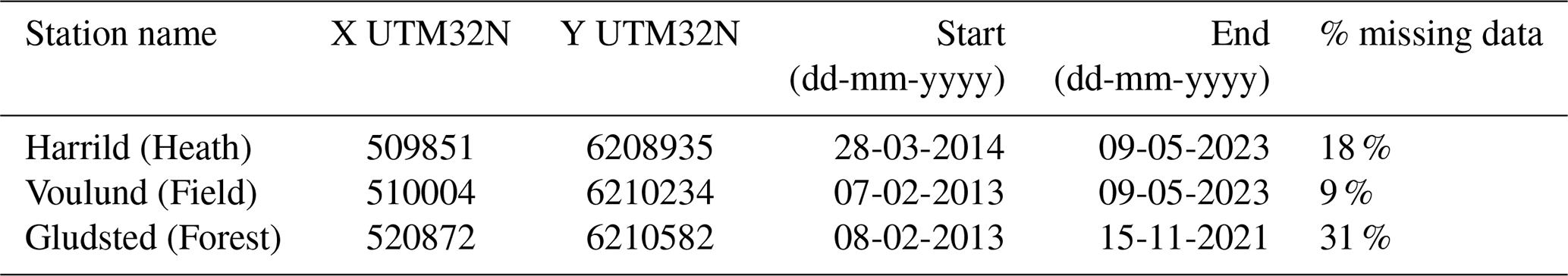
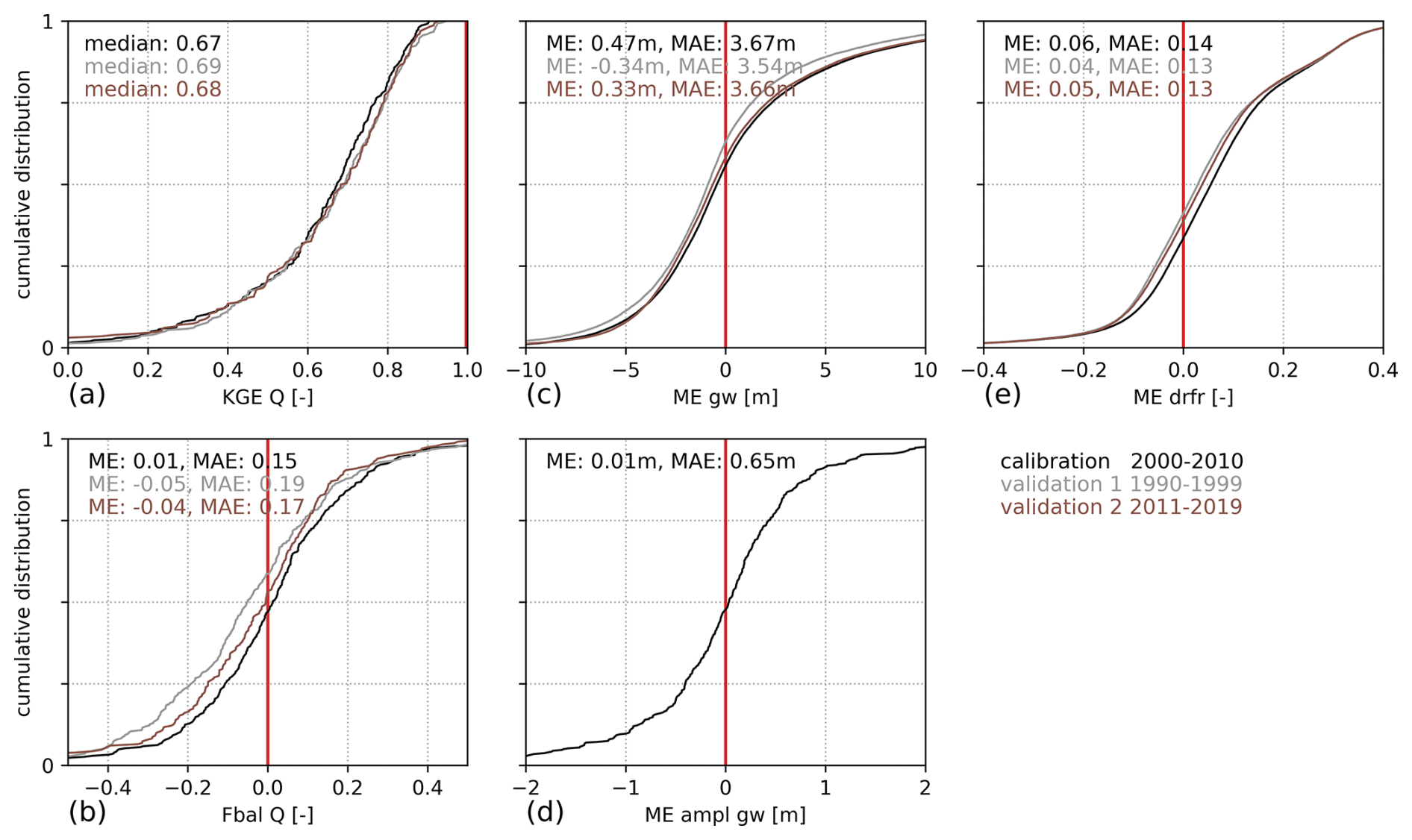
Figure B1 DK-model calibration and validation performance. (a) KGE [–] and (b) water balance error [–] for 305, 278, and 231 stream flow stations for calibration, validation 1 and validation 2 periods, respectively. (c) Residuals against groundwater level measurements in 39 514, 24 862, and 58 059 wells for calibration, validation 1 and validation 2 periods, respectively. (d) Residuals against seasonal groundwater level amplitudes in 400 wells (amplitude dataset required manual filtering which only was performed for calibration period). (e) Residual against ML predictions of drain fraction. Optimal values marked with red.

Appendix C: Accumulation periods using SPEI instead SPI

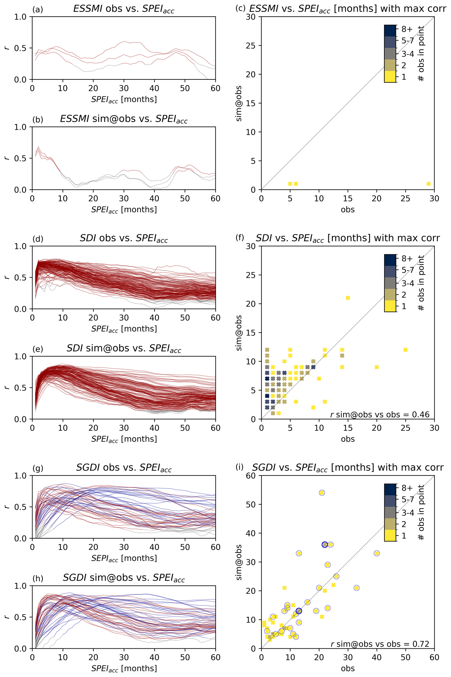
Figure C1 (Equivalent to Fig. 5, but using SPEI instead of SPI.) Left column: correlation coefficients of SPEI accumulation periods against observed and simulated time series of ESSMI (a, b), SDI (d, e) and SGDI (g, h), respectively. Significant correlations (p < 0.01) in red (or blue for wells representing SGDI_deep), remaining in grey. Right column: scatter plots of optimal accumulation period of SPEI for correlation to ESSMI at the 3 CRN stations (c), SDI at the 153 streamflow stations (f), and SGDI at the 53 groundwater wells (i), where wells representing SGDI_deep are marked with blue outlines (two wells in same point: thick blue outline). Optimal SPEI accumulation period for simulated time series along y axis, and for observed time series along x axis.

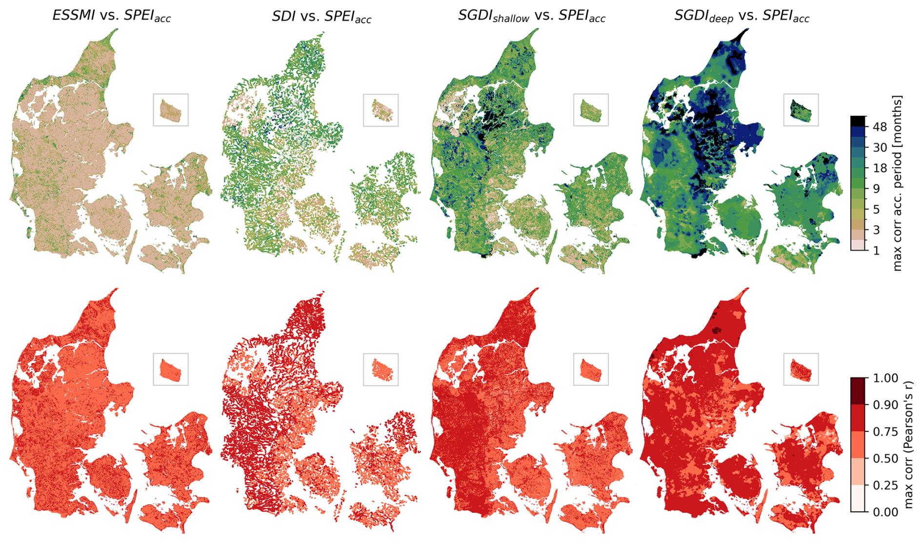
Figure C2 (Equivalent to Fig 6, but using SPEI instead of SPI.) Top row: accumulation period of SPEI_acc yielding maximum correlation with hydrological drought index per DK-model q-point or grid. Bottom row: maximum correlation between hydrologic drought index and SPEI_acc of respective accumulation period. Non-significant correlations (p > 0.01) are masked grey (e.g. isolated areas for SDI and SGDI_deep in eastern Jutland).

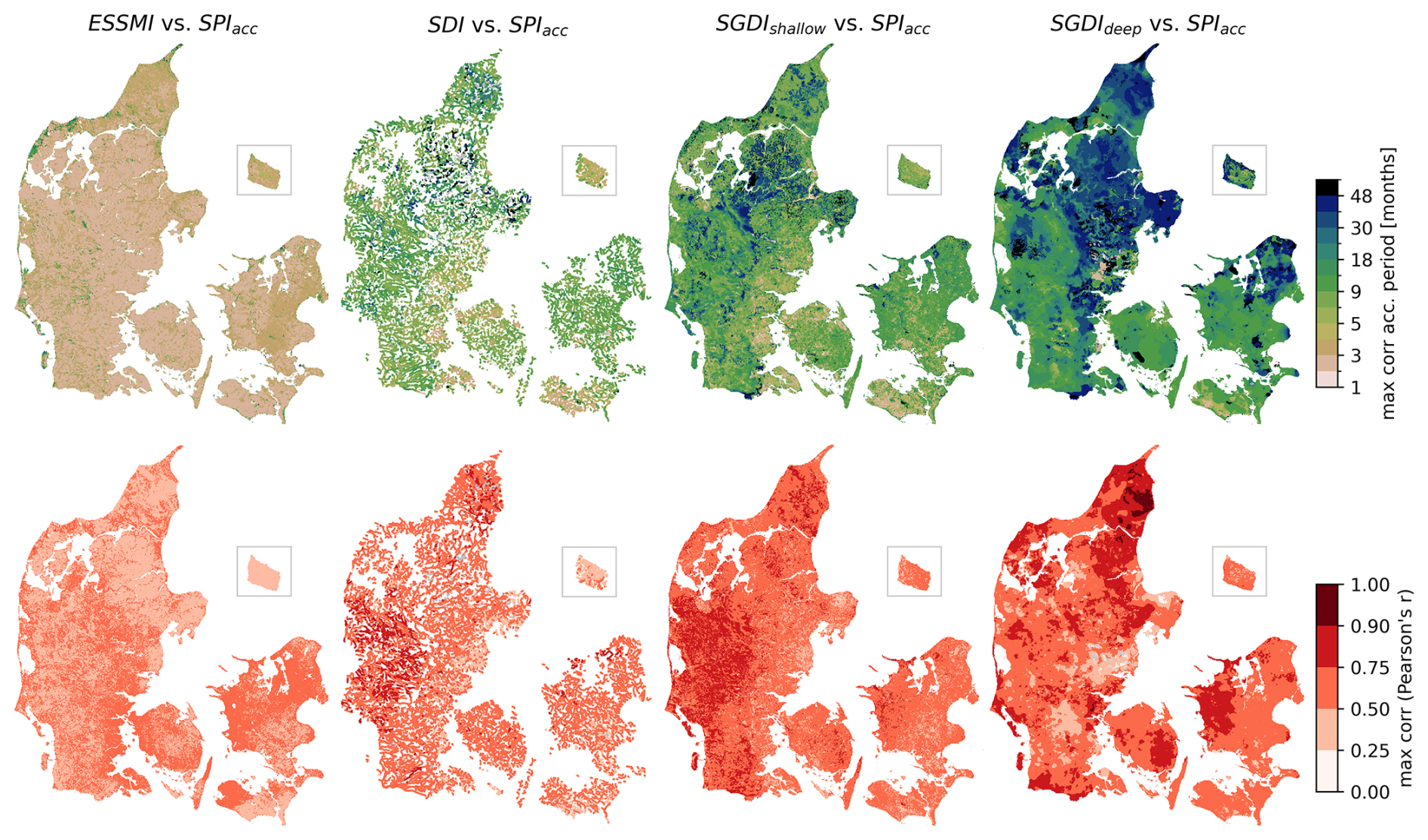
Figure C3 (Equivalent to Fig. 6, but using only data during dry anomalies defined by SPI < 0.) Top row: accumulation period of SPIacc yielding maximum correlation with hydrological drought index per DK-model q-point or grid. Bottom row: Maximum correlation between hydrologic drought index and SPIacc of respective accumulation period. Non-significant correlations (p > 0.01) are masked grey (e.g. isolated areas for SDI and SGDIdeep in eastern Jutland).

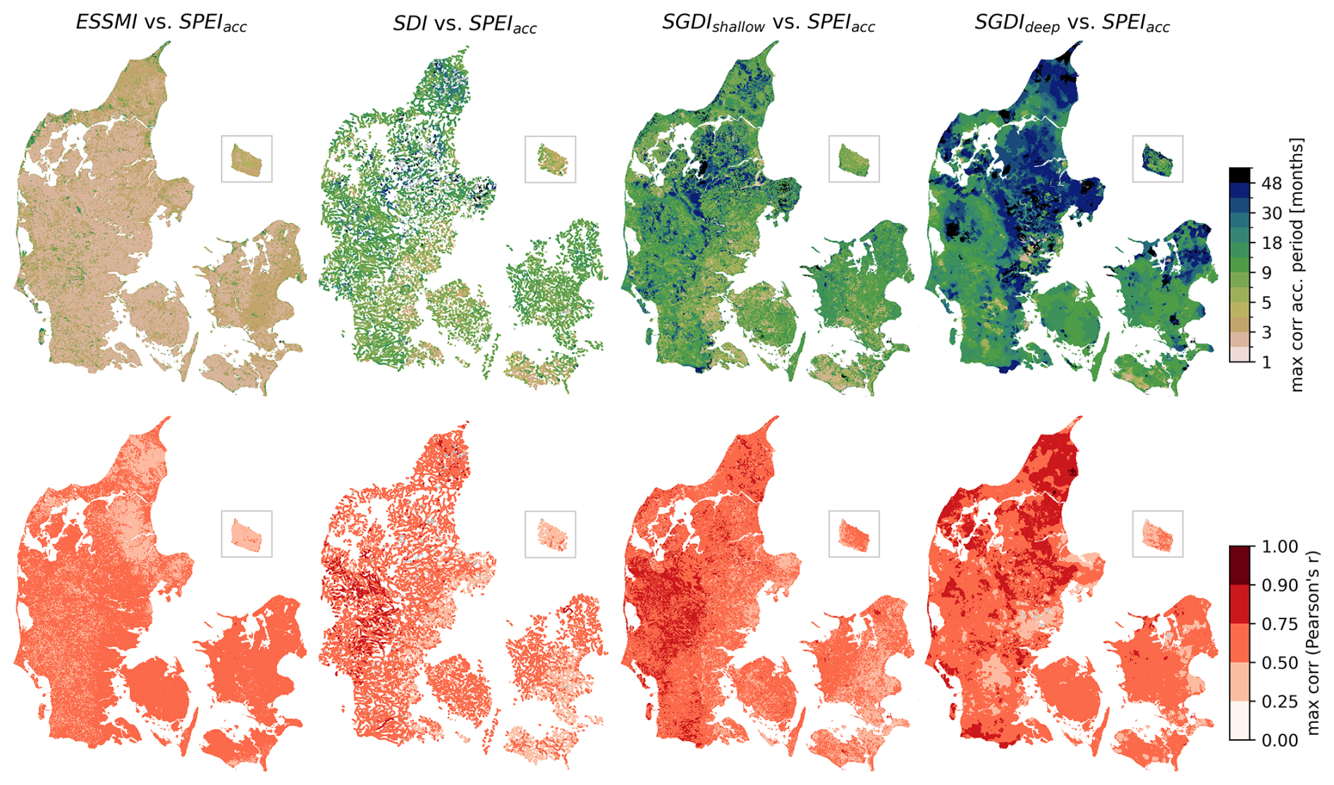
Figure C4 (Equivalent to Fig. 6, but using SPEI instead of SPI and only during dry anomalies defined by SPEI < 0.) Top row: accumulation period of SPEI_acc yielding maximum correlation with hydrological drought index per DK-model q-point or grid. Bottom row: maximum correlation between hydrologic drought index and SPEI_acc of respective accumulation period. Non-significant correlations (p > 0.01) are masked grey (e.g. isolated areas for SDI and SGDI_deep in eastern Jutland).