Daily drought prediction in the Huaihe River Basin using VMD-informer-LSTM

Accurate drought prediction is a key challenge in water resource management and agricultural planning. This study proposes a novel drought prediction framework that integrates Variational Mode Decomposition (VMD), Informer, and Long Short-Term Memory (LSTM) networks to enhance hydrological drought forecasting in the Huaihe River Basin, China. The VMD-Informer-LSTM model decomposes complex non-stationary drought sequences into multi-scale components, effectively extracting long-term trends and short-term fluctuations. Results show that the model outperforms LSTM, Transformer-LSTM, and Informer-LSTM, improving R², RMSE, MAE, and MAPE by 28.4 %, 46.2 %, 46.5 %, and 50.8 %, respectively, over the baseline LSTM. When the prediction period is 30 d, the VMD-Informer-LSTM achieves the highest prediction accuracy. During the 120–180 d prediction period, the prediction accuracy of all models declines, with drought intensity generally underestimated. Misclassifications are mainly concentrated in the transition zones between humid and semi-humid regions, with higher error frequency in semi-humid areas. Prediction accuracy is highest in the upstream and downstream regions, followed by the Yishuisi River Basin, while the midstream region performs poorly due to human interference. Shapley Additive Explanations (SHAP) further reveal that precipitation and temperature are the dominant meteorological drivers, jointly accounting for nearly half of the model's predictive power. These results confirm that the VMD-Informer-LSTM provides the most accurate predictions among the tested models, offering valuable support for drought risk assessment and water resource management in the Huaihe River Basin and other similar regions.

1 Introduction

Drought represents one of the most spatially extensive, temporally persistent, and far-reaching natural disasters globally, with complex formation mechanisms involving intricate interactions between atmospheric circulation patterns, land surface processes, and human activities (Alsubih et al., 2021; Dai, 2013). Drought events not only directly threaten watershed water security and agricultural productivity but also profoundly affect regional ecosystem stability and socioeconomic development (Zhang et al., 2018). With intensifying climate change and increasing human activity intensity, drought events exhibit significant upward trends in frequency, intensity, and spatial extent (Cook et al., 2020; Trenberth et al., 2014). Therefore, accurate drought prediction is crucial for developing scientific disaster mitigation strategies, optimizing water resource allocation schemes, and ensuring regional food and ecological security.

However, drought prediction faces major challenges due to the inherent complexity of drought phenomena (Hao et al., 2017). Drought occurrence and evolution are controlled by multiple natural and anthropogenic factors, including precipitation distribution, evapotranspiration processes, topographic conditions, land use changes, and human interventions (AghaKouchak et al., 2015; Vicente-Serrano et al., 2018). These factors generate highly complex, nonlinear, and non-stationary spatiotemporal evolution patterns. Drought time series typically contain multi-scale periodic oscillations, long-term trend changes, and stochastic fluctuation components that are mutually coupled and interdependent, forming extremely complex dynamical systems (Belayneh et al., 2014; Huang et al., 2015).

Traditional drought prediction methods rely on physics-based numerical models and statistical regression approaches (Dutra et al., 2014; Yuan and Quiring, 2017). Physics-based methods include Global Climate Models (GCMs) such as the ECMWF and NCEP-CFSv2, which can provide global-scale long-term climate predictions but have coarse spatial resolutions (typically 100–200 km) and cannot adequately capture regional drought characteristics (Saha et al., 2014). Regional Climate Models (RCMs) employ dynamic downscaling techniques to achieve high resolutions (10–50 km) but inherit systematic biases from driving models and require substantial computational resources (Jacob et al., 2014; Rummukainen, 2010). Land surface models such as Variable Infiltration Capacity (VIC), Community Land Model (CLM), and Noah simulate coupled water cycle, energy balance, and vegetation dynamics processes but are highly sensitive to meteorological forcing data quality and parameterization schemes (Ek et al., 2003; Lawrence et al., 2011). Statistical methods include linear regression approaches, time series analysis and spectral/wavelet analysis techniques, etc (Box et al., 2015; Modarres, 2007). Time series models, such as Autoregressive Moving Average (ARMA), Autoregressive Integrated Moving Average (ARIMA) models, Random Forest (RF), demonstrate certain capabilities for stationary time series. However, their prediction performance significantly deteriorates on non-stationary, multi-periodic drought sequences (Mishra and Desai, 2005; Mossad and Alazba, 2015). Despite contributions from these traditional methods, fundamental limitations persist across both physics-based and statistical approaches (Hao et al., 2017; Morid et al., 2006). Rigid model structures in both GCMs and RCMs cannot adaptively adjust to accommodate intrinsic data characteristics. Insufficient nonlinear processing capabilities in land surface models and statistical methods (including ARMA, ARIMA, and RF models) cannot capture complex feedback mechanisms and threshold effects (AghaKouchak et al., 2015). Additionally, there are difficulties in multi-scale information integration and heterogeneous data fusion, particularly in land surface models and GCMs (Wood et al., 2016). High parameter sensitivity affects the robustness and generalization capability of both physics-based and statistical models (including ARMA, ARIMA, and RF models) (Svoboda et al., 2002). Finally, trade-offs between computational efficiency and accuracy challenge the operational implementation requirements of RCMs and complex statistical models (Mo, 2008; Yuan and Quiring, 2017).

Recent advances in artificial intelligence and big data technologies have fundamentally transformed time series modeling and prediction across multiple fields (LeCun et al., 2015; Shlezinger et al., 2023). Deep learning methods demonstrate significant advantages in automatically capturing complex patterns and latent features without requiring pre-specified physical relationships, possessing powerful nonlinear mapping and adaptive learning capabilities (Bengio et al., 2013; Schmidhuber, 2015). Long-Short-Term Memory (LSTM) networks have been successfully applied to various hydrological nonlinear sequence modeling tasks, including streamflow prediction, flood forecasting, and water level estimation, demonstrating superior predictive performance (Kratzert et al., 2018; Zhang et al., 2014). LSTM networks through their unique gate mechanisms and memory cell design effectively address gradient vanishing problems in traditional recurrent neural networks and exhibit excellent performance in capturing long-term dependency information (Greff et al., 2017). However, single deep learning architectures still have limitations when processing complex time series data, and multi-model ensemble and parallel architecture designs provide novel approaches for further enhancing prediction performance (Mosavi et al., 2018; Sit et al., 2020).

To enhance model capability for processing non-stationary complex sequences, signal decomposition algorithms for data preprocessing have become key strategies for improving time series prediction performance. Variational Mode Decomposition (VMD), an advanced adaptive signal decomposition technique proposed by Dragomiretskiy and Zosso in 2014, decomposes non-linear, non-stationary complex sequences into multiple Intrinsic Mode Functions (IMFs) with different center frequencies. Each IMF reflects the dynamic characteristics of the original sequence at specific frequency levels, possessing relatively independent frequency bandwidth and amplitude modulation properties (Dragomiretskiy and Zosso, 2014). Compared to traditional decomposition methods such as Empirical Mode Decomposition (EMD) and Ensemble EMD (EEMD), VMD is based on rigorous variational optimization theoretical frameworks, employs completely non-recursive decomposition models, effectively avoids mode mixing and end-effect problems, and possesses superior frequency separation effects and noise robustness.

In recent years, Transformer architectures have achieved major breakthroughs in time series prediction, particularly the informer model specifically optimized for long time series prediction tasks. Zhou proposed that informer reduces computational complexity from O (L²) to O (LlogL) through Probabilistic Sparse Self-attention mechanisms, combined with self-attention distillation operations that progressively compress sequence length layer by layer, significantly improving efficiency and accuracy in processing lengthy sequences (Zhou et al., 2021). This innovative architecture provides novel technical pathways for capturing long-range temporal dependencies.

This study adopts the Daily Evapotranspiration Deficit Index (DEDI) as a drought monitoring indicator, constructed based on daily actual and potential evapotranspiration from ERA5 reanalysis data, which can effectively reflect the dynamic evolution processes of regional droughts (Hersbach et al., 2020; Zhang et al., 2022; Zuo et al., 2020). Building upon this foundation, we propose a novel drought prediction model integrating Variational Mode Decomposition, informer, and Long Short-Term Memory networks (VMD-informer-LSTM), which is expected to provide a high-accuracy, robust prediction framework for drought prediction applications by combining the technical advantages of variational optimization decomposition, probabilistic sparse attention mechanisms, and gated memory networks. Through a combination of multiscale feature decomposition and hybrid deep learning architectures, this method effectively handles the non-stationary characteristics of complex drought indices like DEDI, accurately capturing long-range climate trends and short-term fluctuations. This study significantly improved prediction accuracy and reliability of complex non-stationary drought time series and provided scientific foundations for regional water resource management and drought risk assessment (Pozzi et al., 2013; Willmott and Matsuura, 2005).

The technical approach includes: (1) utilizing VMD for adaptive modal decomposition of original DEDI sequences, deconstructing complex nonlinear time series into multi-frequency scale IMF components to achieve structured extraction of multi-scale features (Dragomiretskiy and Zosso, 2014; Johny et al., 2022); (2) constructing dual-branch parallel architecture of informer and LSTM, where informer efficiently captures global trends of long-range sequences through probabilistic sparse attention mechanisms, while LSTM precisely models local temporal dynamics through gating mechanisms (Zhou et al., 2021); (3) fusing dual-source features through fully connected layers to form hybrid feature representations possessing both long-range dependency analysis capability and short-term fluctuation capture ability (Li et al., 2023; Zhang et al., 2019); (4) adopting a three-stage design of decomposition-parallelization-fusion to obtain final drought prediction results.

2 Study Area and data

2.1 Study Area

The Huaihe River Basin originates from the Tongbai Mountains in Nanyang City, Henan Province, China. It is located between 111°55^′–121°20^′ E longitude and 30°55^′–36°20^′ N latitude, covering approximately 270 000 km². The basin is situated in China's north-south climate transition zone, with the area north of the Huaihe River belonging to the warm temperate zone and the area south of the river belonging to the northern subtropical zone (Yao et al., 2024). The annual mean temperature ranges from 11–16 °C, with temperature variations increasing from north to south and from coastal to inland areas. The Huaihe River Basin receives a multi-year average precipitation of 883 mm, with a spatial distribution characterized by higher precipitation in mountainous areas compared to plains, increased precipitation along the coast than inland, and a decreasing gradient from south to north. The multi-year average evaporation in the basin fluctuates between 650–1250 mm, primarily concentrated during May-August, with an overall decreasing trend from south to north and from east to west. The studied region is shown in Fig. 1.

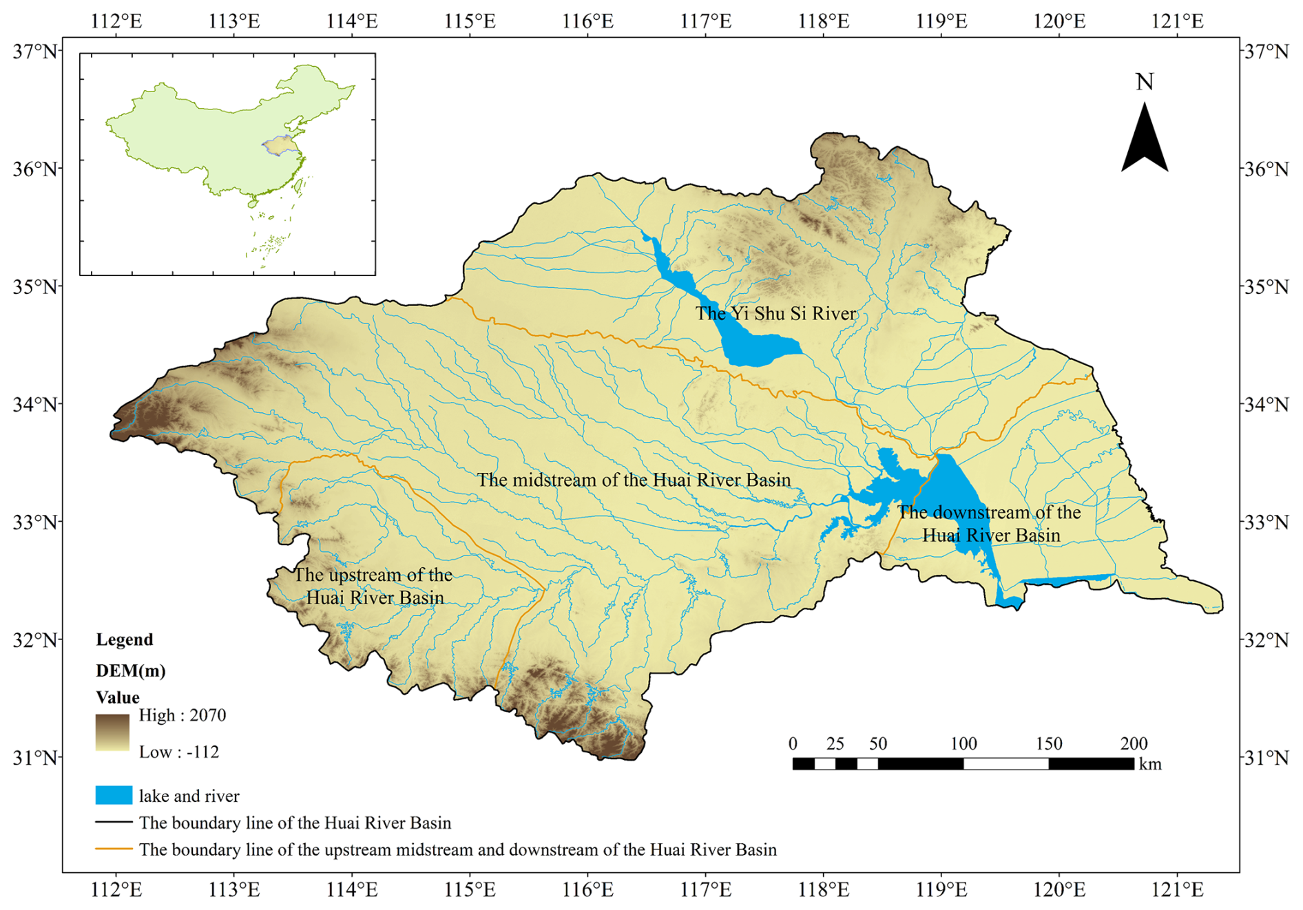
Figure 1 The study area of Huaihe river Basin.

During the 62-year period from 1949 to 2010, the Huaihe River Basin experienced cumulative drought-affected areas of 167 million ha, with disaster-affected areas of 87.3 million ha, resulting in grain losses of 13.96 billion kg. On average, 2.698 million ha of crops were affected by drought annually, with 1.408 million ha suffering disaster-level impacts (Gao et al., 2015). Drought disasters have severely impacted industrial and agricultural production, urban and rural water supply security, and ecological environments within the basin, becoming one of the primary factors constraining rapid and sustainable socio-economic development in the region. Therefore, providing reliable drought prediction methods is of great significance for accurate drought forecasting and the scientific development of drought response strategies in the Huaihe River Basin.

2.2 Data Sources

This study utilizes daily actual evapotranspiration, potential evapotranspiration, surface pressure, cloud cover, maximum temperature, mean temperature, wind speed, and precipitation data for the period 1980–2020, sourced from the fifth-generation high-resolution atmospheric reanalysis product (ECMWF Reanalysis v5, ERA5) developed by the European Centre for Medium-Range Weather Forecasts (ECMWF). ERA5 data are characterized by extensive coverage, long time series, and excellent spatio-temporal consistency. This makes them an optimal data choice for long-term and high-resolution analyses. To meet the specific spatial resolution requirements of this study, the downloaded ERA5 data were further subjected to interpolation processing. This converted them to a spatial resolution of 0.25°×0.25° to more precisely match the spatial characteristics of the study region (Muñoz-Sabater et al., 2021).

Land use data for 2005, 2010, 2015, and 2020 with a spatial resolution of 1 km were obtained from the Data Center for Resources and Environmental Sciences, Chinese Academy of Sciences (https://doi.org/10.12078/2018070201, Xu et al., 2018). Additional details on the data and preprocessing procedures are provided in the Supplement.

3 Methods

3.1 DEDI Index

The Daily Evapotranspiration Deficit Index (DEDI) is a daily drought index constructed based on daily evapotranspiration as well as potential evapotranspiration for monitoring and predicting regional drought events (Zhang et al., 2022). This index is calculated based on ERA5 data provided by ECMWF.

The DEDI is calculated as follows:

$$\begin{array}{}\text{(1)}& {\displaystyle }{\mathrm{DEDI}}_i={\displaystyle \frac{D_i-D_{\mathrm{AVE}}}{D_{\mathrm{STU}}}}\text{(2)}& {\displaystyle }{D}_i={\mathrm{AET}}_i-{\mathrm{PET}}_i\end{array}$$

where i represents time, AET_i represents the actual evapotranspiration on day i (units: mm d⁻¹), PET_i represents the potential evapotranspiration on day i (units: mm d⁻¹), D_i represents the evapotranspiration deficit between AET and PET on day i, and D_AVE and D_STU are the multi-year climatological mean and standard deviation, respectively (Zuo et al., 2020).

3.2 VMD

Variational Mode Decomposition (VMD) was proposed by Konstantin Dragomiretskiy (Dragomiretskiy and Zosso, 2014) as a signal processing method designed to effectively overcome mode mixing and end effect problems existing in Empirical Mode Decomposition (EMD). Unlike the recursive decomposition principle of EMD, VMD determines the central frequency and bandwidth of each mode component. This is done by constructing and solving the optimal solution to a variational model. This represents a completely non-recursive decomposition model. This method searches for a set of mode components and their corresponding center frequencies through an iterative search. This ensures that each mode maintains smoothness after demodulation to baseband.

The adaptivity of VMD is reflected in its ability to automatically determine the number of modes decompositions according to signal characteristics and adaptably match the optimal center frequency and finite bandwidth for each mode, thereby achieving effective separation of Intrinsic Mode Functions (IMFs) and frequency domain partitioning of signals. Experimental results demonstrate that VMD exhibits strong robustness in sampling and noise aspects, is capable of reducing the non-stationarity of time series with high complexity and strong non-linearity and decomposing them into multiple sub-sequences with different frequency scales that are relatively stationary, making it particularly suitable for non-stationary signal processing.

VMD decomposes time series into simple high-frequency and low-frequency intrinsic mode functions through optimization processes, improving signal processing stability and accuracy. This method is not only theoretically innovative but also demonstrates superior performance in practical applications, providing an effective tool for non-stationary signal analysis. Research by Zhao et al. (2023) further proved VMD's excellent performance in handling boundary effects by adjusting parameters (such as decomposition levels, quadratic penalty terms, etc.) to effectively control deviations in decomposition results, thereby improving model adaptability (Zhang et al., 2023; Zhao et al., 2023).

In this study, two key parameters of the Variational Mode Decomposition (VMD) need to be predefined: the penalty factor α (bandwidth constraint parameter) and the number of modes K (i.e., the number of intrinsic mode functions, IMFs). The penalty factor α is empirically determined based on the length of the time series, with its value ranging from 1.5 to 2.0 times the sample length, aiming to balance frequency band separation and decomposition stability. When α is relatively small, the bandwidth of each IMF becomes wider, which may lead to spectral overlap between different modes and thus reduce the physical interpretability of the decomposition results; whereas when α is excessively large, the bandwidth is overly constrained, making the decomposition more sensitive to noise. In this study, α is finally set to 1.75 times the sample length. In addition, the number of modes K is determined based on the frequency distribution characteristics of the decomposed signal and preliminary experimental results. When K is less than 7, certain IMF components exhibit significant spectral mixing, making it difficult to effectively separate signals at different time scales; when K exceeds 7, the center frequencies of adjacent IMFs become too close and the energy distribution tends to be dispersed, resulting in redundant or noise-dominated modes and thus reducing the stability and physical interpretability of the decomposition. Therefore, K is uniformly set to 7 in this study to ensure effective separation of the dominant frequency components of the original DEDI series while avoiding redundancy caused by over-decomposition. Preliminary experiments conducted on several representative grid points indicate that this parameter combination yields stable decomposition results and satisfactory predictive performance. To maintain methodological consistency and avoid potential spatial overfitting, the same VMD parameter settings are applied uniformly across all grid points in the study area.

Assuming the original signal f is decomposed into k components, ensuring that the decomposed sequences are modal components with finite bandwidth and center frequencies, while minimizing the sum of estimated bandwidths of all modes, with the constraint that the sum of all modes equals the original signal, the VMD constrained variational model is as follows:

$$\begin{array}{}\text{(3)}& \begin{array}{c}min\\ \mathit{\{}{u}_k,{\mathit{\omega }}_k\mathit{\}}\end{array}\left\{\sum _{k=\mathrm{1}}^K\Vert {\partial }_t\left[\left(\mathit{\delta }\left(t\right)+{\displaystyle \frac{j}{\mathit{\pi }t}}\right)*u_k\left(t\right)\right]e^{-j{\mathit{\omega }}_{k}t}{\Vert }_{\mathrm{2}}^{\mathrm{2}}\right\}\text{(4)}& {\displaystyle }\mathrm{s}.\mathrm{t}.\sum _k{u}_k=f\left(t\right)\text{(5)}& {\displaystyle }{u}_k=\mathit{\{}{u}_{\mathrm{1}},u_{\mathrm{2}},\mathrm{\dots },u_k\mathit{\}}\text{(6)}& {\displaystyle }{\mathit{\omega }}_k=\mathit{\{}{\mathit{\omega }}_{\mathrm{1}},{\mathit{\omega }}_{\mathrm{2}},\mathrm{\dots },{\mathit{\omega }}_k\mathit{\}}\end{array}$$

where f(t) represents the original data; K represents the number of modal components; δ(t) represents the Dirac function; * represents convolution operation; ∂_t is the partial derivative operator; {u_k} represents the kth component function obtained through calculation; {ω_k} represents the center frequency of the kth component obtained through calculation.

The augmented LaGrange is introduced to solve this constrained optimization problem:

$$\begin{array}{}\text{(7)}& \begin{array}{rl}& L\left(\mathit{\right\{}{u}_k\mathit{\}},\mathit{\{}{\mathit{\omega }}_k\mathit{\}},\mathit{\lambda })=\mathit{\alpha }\sum _k\Vert {\partial }_t\left[\left(\mathit{\delta }\left(t\right)+{\displaystyle \frac{j}{\mathit{\pi }t}}\right)*u_k\left(t\right)\right]\\ & e^{-j{\mathit{\omega }}_{k}t}{\Vert }_{\mathrm{2}}^{\mathrm{2}}+\Vert f\left(t\right)-\sum _k{u}_k\left(t\right){\Vert }_{\mathrm{2}}^{\mathrm{2}}\\ & +\langle \mathit{\lambda }\left(t\right),f\left(t\right)-\sum _k{u}_k\left(t\right)\rangle \end{array}\end{array}$$

where α represents the penalty factor; λ(t) represents the Lagrange multiplier.

The alternating direction method of multipliers (ADMM) is used to find the saddle point of the augmented LaGrange. In the frequency domain, the updates are:

$$\begin{array}{}\text{(8)}& {\displaystyle }{\widehat{u}}_k^{n+\mathrm{1}}\left(\mathit{\omega }\right)={\displaystyle \frac{\widehat{f}\left(\mathit{\omega }\right)-{\sum }_{i\ne k}^k{\widehat{u}}_k^{n+\mathrm{1}}\left(\mathit{\omega }\right)+\frac{{\widehat{\mathit{\lambda }}}^n\left(\mathit{\omega }\right)}{\mathrm{2}}}{\mathrm{1}+\mathrm{2}\mathit{\alpha }{\left(\mathit{\omega }-{\mathit{\omega }}_k^n\right)}^{\mathrm{2}}}}\text{(9)}& {\displaystyle }{\mathit{\omega }}_k^{n+\mathrm{1}}={\displaystyle \frac{{\int }_{\mathrm{0}}^{\mathrm{\infty }}\mathit{\omega }\mid u_k^{n+\mathrm{1}}\left(\mathit{\omega }\right)\mid \mathrm{d}\mathit{\omega }}{{\int }_{\mathrm{0}}^{\mathrm{\infty }}\mid u_k^{n+\mathrm{1}}\left(\mathit{\omega }\right)\mid \mathrm{d}\mathit{\omega }}}\text{(10)}& {\displaystyle }{\widehat{\mathit{\lambda }}}^{n+\mathrm{1}}\left(\mathit{\omega }\right)\leftarrow {\widehat{\mathit{\lambda }}}^n\left(\mathit{\omega }\right)+\mathit{\pi }\left[\widehat{f}\left(\mathit{\omega }\right)-\sum _{i\ne k}{\widehat{u}}_k^{n+\mathrm{1}}\left(\mathit{\omega }\right)\right]\end{array}$$

where γ represents noise tolerance; the ${\widehat{u}}_k^{n+\mathrm{1}}\left(\mathit{\omega }\right)$ represent Wiener filtering residuals; ${\widehat{u}}_i\left(\mathit{\omega }\right)$ and ${\widehat{\mathit{\lambda }}}^n\left(\mathit{\omega }\right)$ represent the Fourier transforms of u(t) and λ(t), respectively.

3.3 LSTM

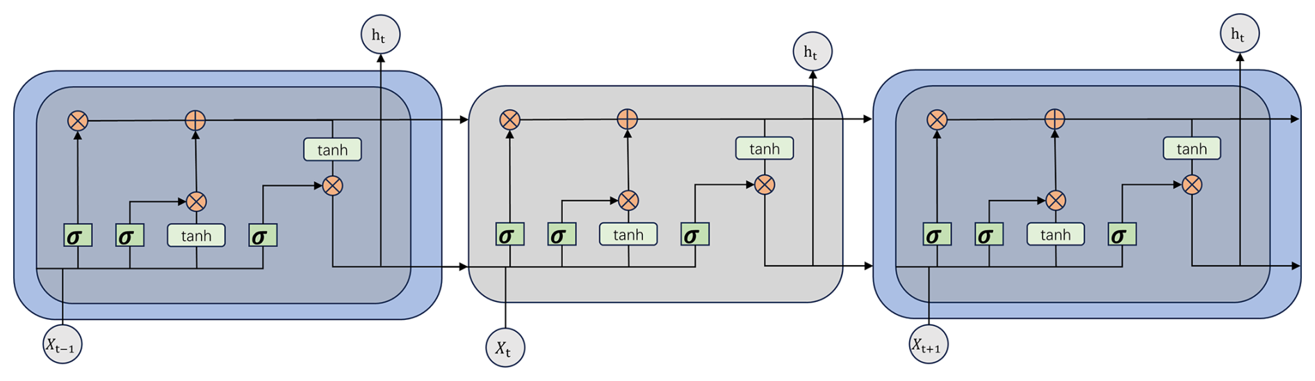
The Long-Short-Term Memory (LSTM) models are a special type of Recurrent Neural Network (RNN) variant that addresses the gradient vanishing problem in RNN processing of long sequence data by introducing memory cells (Cell States), specifically designed for processing time series data (Hochreiter and Schmidhuber, 1997). When recording long sequence data, RNN experiences gradient vanishing or exploding due to continuous information accumulation, making it difficult for the network to learn long-term dependencies, ultimately affecting the model's accurate capture of trends and periodicity in time series data (Jaseena and Kovoor, 2022).

LSTM aims to solve the gradient-vanishing or exploding problems encountered by traditional RNN when processing long sequence data. This is done mainly through gate mechanisms regulating information flow. The LSTM model consists of four interacting layers: input gate, forget gate, cell state gate, and output gate. It is shown in Fig. 2 below.

Figure 2 The construction of LSTM.

3.4 Informer

Informer is an improved and optimized version based on Transformer, specifically designed to enhance the speed and efficiency of processing long sequences and optimized for long-term time series prediction tasks (Zhou et al., 2021). Transformer captures relationships between different positions in sequences through Self-Attention mechanisms. However, Transformer encounters difficulties when processing long time series data because its computational complexity grows quadratically with sequence length, becoming very slow or even unprocessable when dealing with very long time series.

Informer proposes ProbSparse Self-attention to filter critical queries and reduce computational complexity, and introduces Self-attention Distilling to reduce dimensions and network parameters (Vaswani et al., 2017). As shown in Fig. 3, the informer architecture consists of an encoder-decoder structure. Input sequences first undergo convolutional encoding and positional embedding before being fed into the encoder; the encoder utilizes multi-layer probabilistic sparse self-attention and distillation operations to extract key information, outputting encoded features. The decoder then directly generates long sequence predictions under masked self-attention and cross-attention, followed by fully connected layers mapping to final values.

Figure 3 The construction of the informer.

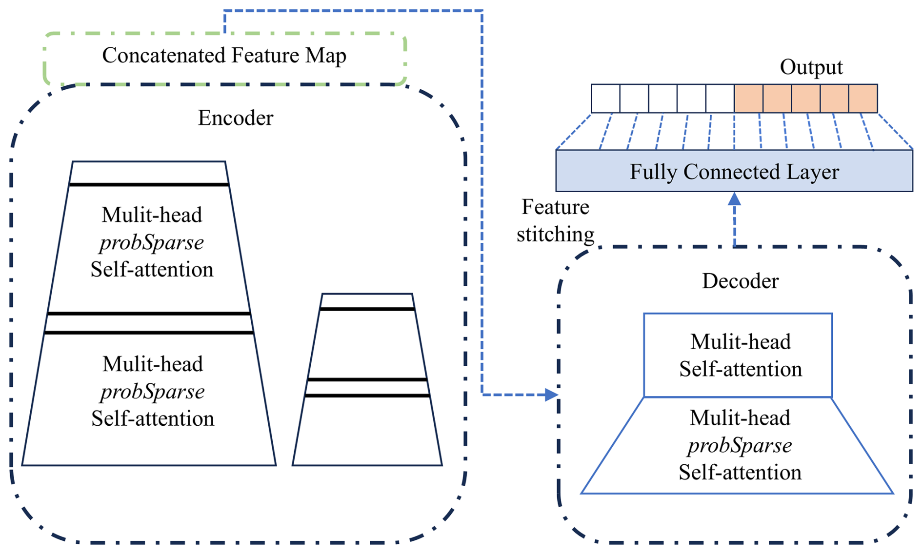
For long sequence prediction, the informer has three advantages: (1) Probabilistic sparse self-attention reduces time complexity from O (L²) to O (LlogL), significantly reducing computational overhead; (2) self-attention distillation progressively compresses the sequence length layer by layer, simultaneously reducing computation and memory requirements; (3) generative decoding outputs complete future sequences at once, avoiding error accumulation caused by step-by-step extrapolation.

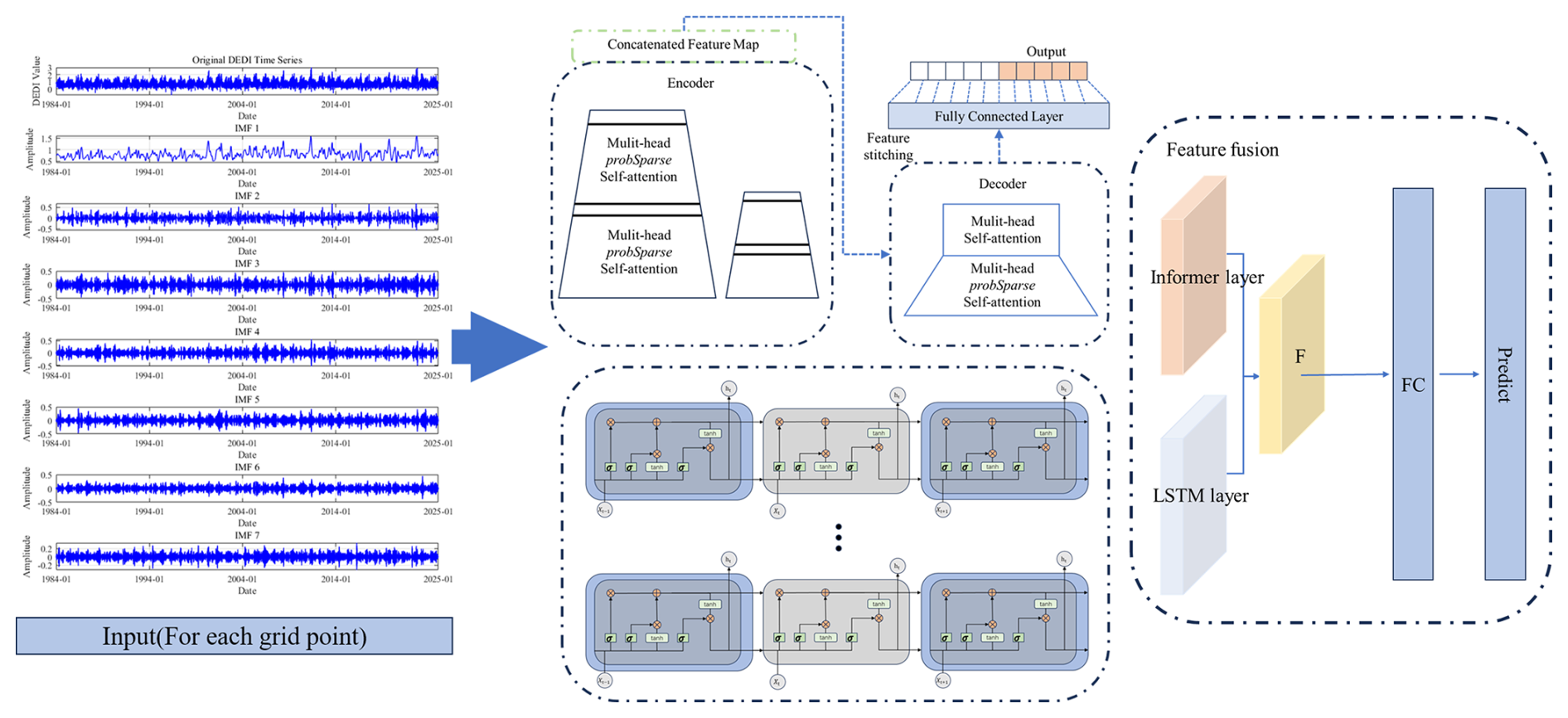
3.5 VMD-informer-LSTM

The VMD-informer-LSTM model employs Variational Mode Decomposition (VMD) to deconstruct DEDI time series into multi-frequency scale Intrinsic Mode Functions (IMFs), achieving the structured extraction of multi-scale features. Based on this foundation, it constructs a dual-branch parallel architecture of informer and LSTM, where informer efficiently captures global trends of long-range sequences through probabilistic sparse attention mechanisms, while LSTM precisely models local temporal dynamics through gate mechanisms. Finally, dual-source features are fused through fully connected layers to form hybrid feature representations possessing both long-range dependency analysis capability and short-term fluctuation capture ability. This model significantly improves prediction accuracy and reliability for complex time series data through a three-stage design of decomposition-parallelization-fusion, providing an innovative solution for time series prediction tasks. The construction of VMD-informer-LSTM is shown in Fig. 4 below.

Figure 4 The construction of VMD-informer-LSTM.

Building upon this foundation, in order to ensure the standardization of the model training process and the reproducibility of the results, this study further establishes a unified design for dataset partitioning and hyperparameter optimization procedures. For the DEDI time-series data at each grid point, the dataset is strictly divided in chronological order using a forward-splitting strategy to prevent any potential leakage of future information. Specifically, the training period spans from 1 January 1984 to 3 July 2024, while the testing period covers 4 July 2024 to 31 December 2024, which is used to evaluate the model's predictive performance on unseen data over the subsequent 180 d forecasting horizon. It should be noted that the 180 d prediction in this study does not correspond to traditional deterministic weather forecasting, but rather focuses on predicting the evolution of drought states.

Regarding hyperparameter configuration, this study adopts the Bayesian Optimization method to automatically search for key hyperparameters (including hidden layer dimension, learning rate, and batch size) within a predefined parameter search space. Each candidate parameter combination is evaluated based on its predictive performance on the validation set, with the minimization of validation error serving as the optimization objective function. The optimal parameter combination is then selected for the final model training and testing evaluation. Through the design of the above training strategy and hyperparameter optimization procedure, the experimental process ensures methodological rigor, stability of results, and reproducibility of the research.

3.6 Shapley Additive Explanations

Since machine learning models are “black-box” models, although they can provide efficient predictions, their internal decision-making processes are complex and difficult to intuitively understand and explain. This may affect result analyses in the field of raster data, which require transparency and interpretability. To overcome such problems, SHAP values are introduced as an interpretive method. The SHAP value method was proposed by Lundberg et al (Lundberg and Lee, 2017). In 2017, it is a method based on cooperative game theory that quantifies the contribution of driving factors to model prediction results. By calculating the marginal contributions of each factor to the model output under different combinations, it measures their importance in the overall prediction results. This helps us understand how the model makes decisions. The positive or negative values of SHAP indicate promotion or inhibition of prediction results. The absolute value reflects the degree of influence of the factor on the model prediction results. The larger the absolute value, the greater the influence of the factor on model prediction results (Wang et al., 2024). The formula is as follows:

$$\begin{array}{}\text{(11)}& {\mathit{\varphi }}_i=\sum _{S\in N\setminus \mathit{\left\{}i\mathit{\right\}}}{\displaystyle \frac{\mathrm{|}S\mathrm{|}\mathrm{!}(\mathrm{|}N\mathrm{|}-\mathrm{|}S\mathrm{|}-\mathrm{1})\mathrm{!}}{\mathrm{|}N\mathrm{|}\mathrm{!}}}[f\left(S\cup \left\{i\right\}\right)-f\left(S\right)]\end{array}$$

In the formula, ϕ_i represents the SHAP value for feature i; N is the set of all features; S is a subset of features, excluding feature i; f(S) is the model output using only the feature subset S for prediction; (f(S∪{i}) is the predicted value after adding feature i to the featured subset S.

3.7 Evaluation Metrics

The coefficient of determination (R²) measures the proportion of variance in the dependent variable that is derived from the independent variable, ranging from 0 to 1, where values closer to 1 indicate better model performance (Nash and Sutcliffe, 1970). The root mean square error (RMSE) quantifies the average magnitude of prediction errors, providing a measure of how well the model predicts actual values, with lower values indicating better accuracy (Willmott and Matsuura, 2005). Mean absolute error (MAE) represents the average absolute difference between predicted and observed values, offering a linear score that is less sensitive to outliers than RMSE. The range of mean absolute percentage error (MAPE) is [0, +∞]. A MAPE of 0 % indicates a perfect model, while a MAPE greater than 100 % suggests a poor model (Myttenaere et al., 2016).

The mathematical expressions for these metrics appear as follows:

$$\begin{array}{}\text{(12)}& {\displaystyle }{R}^{\mathrm{2}}=\mathrm{1}-{\displaystyle \frac{\mathrm{SSE}}{\mathrm{SST}}}=\mathrm{1}-{\displaystyle \frac{{\sum }_{i=\mathrm{1}}^N(y_{\mathrm{obs}}-y_{\mathrm{pred}}{)}^{\mathrm{2}}}{{\sum }_{i=\mathrm{1}}^N\mathrm{\Sigma }(y_{\mathrm{obs}}-{\widehat{y}}_{\mathrm{obs}}{)}^{\mathrm{2}}}}\text{(13)}& {\displaystyle }\mathrm{RMSE}=\sqrt{{\displaystyle \frac{\mathrm{1}}{N}}\sum _{i=\mathrm{1}}^N(y_{\mathrm{obs}}-y_{\mathrm{pred}}{)}^{\mathrm{2}}}\text{(14)}& {\displaystyle }\mathrm{MAE}={\displaystyle \frac{\mathrm{1}}{N}}\sum _{i=\mathrm{1}}^N\left|y_{\mathrm{obs}}-y_{\mathrm{pred}}\right|\text{(15)}& {\displaystyle }\mathrm{MAPE}={\displaystyle \frac{\mathrm{1}}{N}}-\sum _{i=\mathrm{1}}^N\mathrm{abs}\left({\displaystyle \frac{y_{\mathrm{obs}}-y_{\mathrm{pred}}}{y_{\mathrm{obs}}}}\right)\end{array}$$

where y_obs represents observed values, y_pred represents predicted values, ${\widehat{y}}_{\mathrm{obs}}$ is the mean of observed values, and n is the number of observations.

4 Results

4.1 VMD Decomposition Results

In this study, we systematically selected 108 grid points distributed across the Huaihe River Basin and performed VMD analysis of their corresponding daily DEDI time series data spanning 1980–2020. Figure 5 provides a comprehensive visual representation of the decomposed sub-sequences of DEDI data for a certain representative grid cell in the Huaihe River Basin. As illustrated in Fig. 5, the daily DEDI values for a representative grid cell in the Huaihe River Basin exhibit substantial positive and negative fluctuations, with considerable variance between maximum and minimum values. These pronounced oscillations present significant challenges in capturing essential features during the prediction process, as the complex, non-stationary nature of the original signal obscures the underlying patterns and trends. The VMD algorithm successfully decomposes the complex, non-linear DEDI time series into multiple distinct IMFs, each characterized by specific frequency bands and temporal scales. These decomposed components reveal multi-scale variability patterns ranging from high-frequency short-term fluctuations to low-frequency long-term trends, facilitating more effective feature extraction and modeling processes. VMD technology demonstrates superior capability in accurately tracking changes in signal frequency components and effectively revealing the intrinsic and dynamic characteristics of time series, thereby substantially enhancing prediction accuracy and reliability.

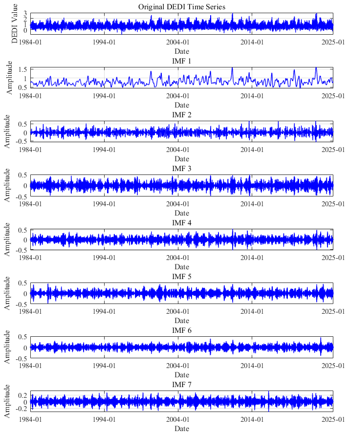
Figure 5 The daily DEDI values of a certain grid in the Huaihe River Basin are decomposed into 7 sub-sequence through variational mode decomposition (VMD).

4.2 Model Prediction Performance Evaluation

To evaluate the performance of the proposed VMD-informer-LSTM model, we performed extensive comparative experiments involving four distinct modeling approaches: the proposed VMD-informer-LSTM model, the informer-LSTM model, the Transformer-LSTM model, and the standalone LSTM model. The evaluation of each model's performance was based on four widely used statistical metrics for time series prediction evaluation. From Table 1, it can be seen that the VMD-informer-LSTM model performs the best in terms of predictive performance, with R², RMSE, MAE, and MAPE reaching 0.9191, 0.1122, 0.0778, and 0.4056, respectively. In contrast, the informer-LSTM model without VMD decomposition has R², RMSE, MAE, and MAPE of 0.8570, 0.1498, 0.1031, and 0.5330, respectively. After calculation, VMD decomposition improves R², RMSE, MAE, and MAPE by 7.25 %, 25.10 %, 24.54 %, and 23.90 %, respectively. Furthermore, the traditional LSTM model shows relatively low predictive accuracy with four evaluation metrics of R²=0.7156, RMSE = 0.2087, MAE = 0.1454, and MAPE = 0.8254. The Transformer-LSTM model achieves R², RMSE, MAE, and MAPE of 0.8286, 0.1641, 0.1130, and 0.6266, respectively. This, although better than the basic LSTM model, is still not as good as the informer-LSTM model, let alone the VMD-informer-LSTM model. In summary, by comparing the predictive performance of the four models, it is evident that the VMD-informer-LSTM model has an advantage in time series prediction tasks. Especially after the introduction of VMD decomposition, its performance has significantly improved, further verifying the effectiveness of VMD decomposition in enhancing model predictive accuracy.

Table 1 Overall average evaluation indicators of various models within the Huaihe River Basin.

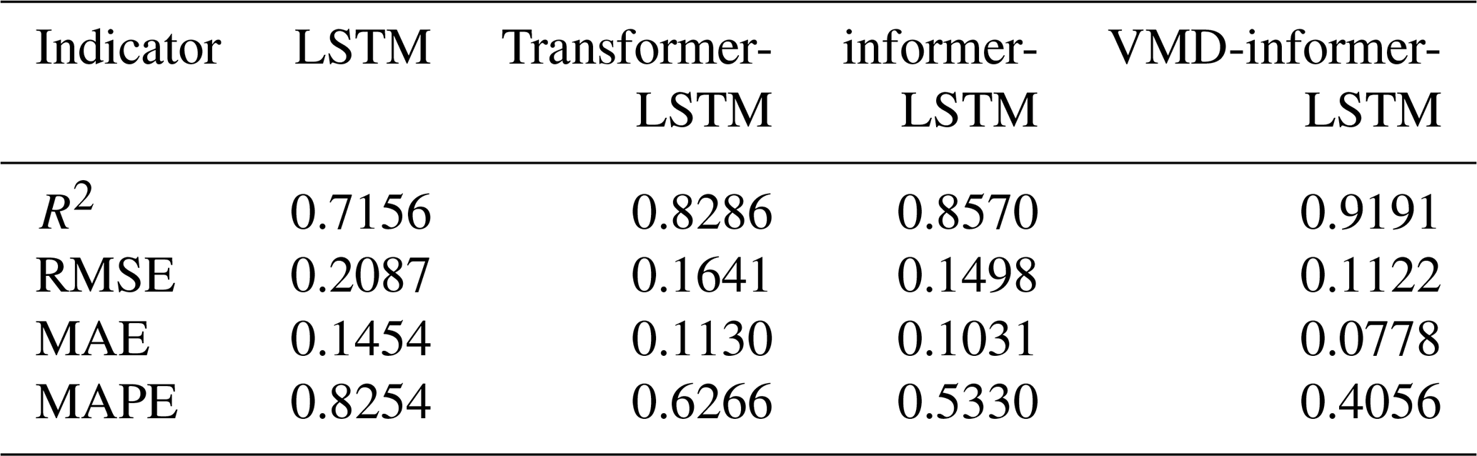
Figure 6 presents violin plots illustrating the distribution of evaluation metrics across all 108 grid points in the Huaihe River Basin. This provides insights into model performance variability and consistency. Violin plots reveal important patterns. The VMD-informer-LSTM model demonstrates the most concentrated distribution around optimal values, with R² distributions tightly clustered near 0.92–0.95, indicating consistent and high performance across diverse geographical locations. Error metric distributions (RMSE, MAE and MAPE) show the VMD-informer-LSTM model has the narrowest spread and the lowest median values, suggesting robust prediction accuracy with minimal spatial variability.

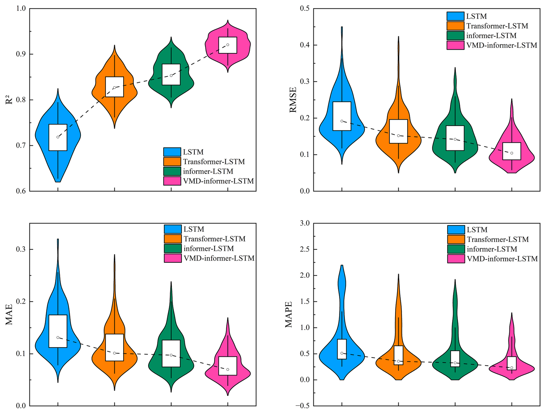
Figure 6 Violin-box plots of evaluation indicators for different models in the Huaihe River Basin.

The RMSE distributions demonstrate a clear monotonic improvement from LSTM (median: 0.2087) through Transformer-LSTM (0.1641), informer-LSTM (0.1498) to VMD-informer-LSTM (0.1122), with progressively narrower interquartile ranges and fewer outliers. The VMD-informer-LSTM model exhibits the most concentrated distribution with minimal dispersion (IQR: 0.05), indicating superior prediction accuracy and enhanced stability across diverse geographical locations. This concentrated performance distribution reflects the effectiveness of combining VMD decomposition with hybrid deep learning architectures for robust drought prediction.

Comparing the four models, the VMD-informer-LSTM model consistently outperforms the other three, with spatially averaged performance metrics across all 108 grid points in the Huaihe River Basin, including an R² of 0.9191, RMSE of 0.1122, MAE of 0.0778, and MAPE of 0.4056. The informer-LSTM model without VMD decomposition has spatially averaged metrics across all grid points of R²=0.8570, RMSE = 0.1498, MAE = 0.1031, and MAPE = 0.5330. The Transformer-LSTM model achieves spatially averaged metrics of R²=0.8286, RMSE = 0.1641, MAE = 0.1130, and MAPE = 0.6266, while the basic LSTM model shows the lowest performance, with spatially averaged metrics of R²=0.7156, RMSE = 0.2087, MAE = 0.1454, and MAPE = 0.8254.

The performance improvement from LSTM to Transformer-LSTM to informer-LSTM is evident, with each model showing better median values and reduced spread in the error metrics compared to the previous one. However, the VMD-informer-LSTM model stands out with the most significant enhancements in both median performance and reduced variance across all metrics. This indicates that the integration of VMD decomposition with the informer-LSTM architecture provides the most substantial benefits in terms of prediction accuracy and consistency.

Figure S5 in the Supplement and 7 show scatter plots and line charts of different models' 180 d predictions in different Huaihe River Basin regions. As illustrated in Fig. S5, LSTM yields the lowest R² values (0.76–0.78) across all subplots and is therefore the poorest performer; its scatter points visibly diverge from the 1:1 line, reflecting the largest prediction errors. Although informer-LSTM is less accurate than VMD-informer-LSTM, it maintains a stable R² of about 0.89, and the scatter deviation is markedly smaller than those of Transformer-LSTM and LSTM.

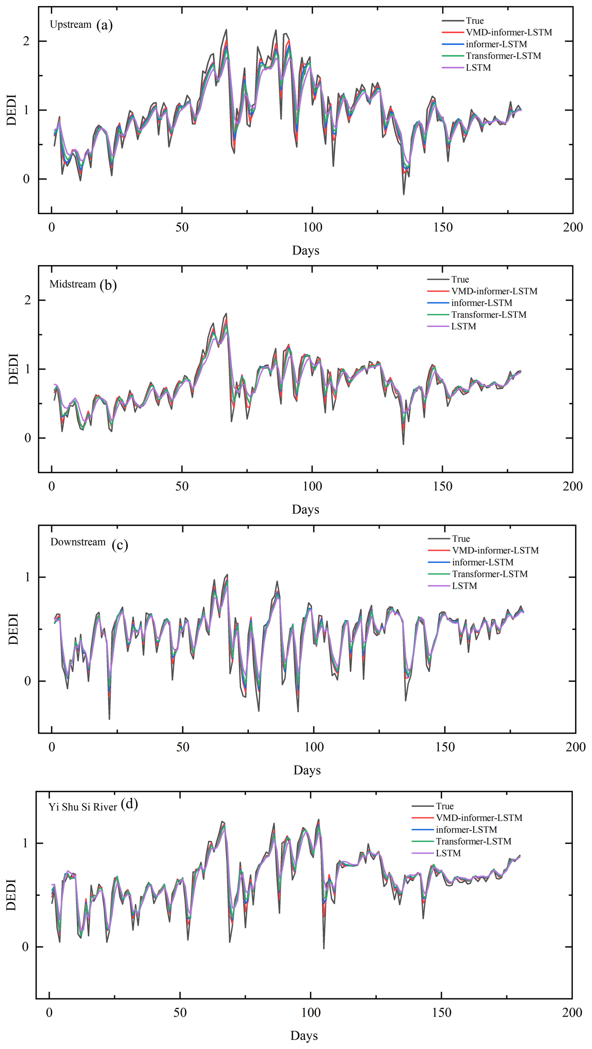
Figure 7 Line charts of different models' 180 d predictions in four Huaihe River Basin Regions: (a) Upstream; (b) Midstream; (c) Downstream; (d) Yi Shu Si River.

Figure 7 further indicates that all four models successfully capture the overall drought trend, yet differ in precision. When the line plots are examined in conjunction, it becomes clear that VMD-informer-LSTM outperforms the other three models, delivering superior agreement between simulated and ERA5 reanalysis values, higher prediction accuracy, and the best overall performance. informer-LSTM and Transformer-LSTM rank next, whereas LSTM only roughly reproduces the drought trend and performs poorly at predicting extremes, resulting in the lowest predictive capability.

Figure 8 presents Taylor diagrams that evaluate the predictive performance of various models across different lead times: (a) 7, (b) 15, (c) 30, (d) 60, (e) 120, and (f) 180 d. These diagrams provide a comprehensive assessment by integrating standard deviation and correlation coefficients from the ERA5 reanalysis data. The VMD-informer-LSTM model consistently shows superior predictive accuracy across all lead times, with its predictions closely aligned with the ERA5 reanalysis data, particularly in the upper, middle, and lower regions of the Huaihe River Basin and the Yi Shu Si River regions. At short lead times (7 and 15 d), all models perform relatively well, but the VMD-informer-LSTM model slightly outperforms the others. As the lead time extends to 30 and 60 d, the VMD-informer-LSTM model maintains high accuracy while other models show performance degradation, indicating a reduced ability to capture the underlying data patterns effectively. At long lead times (120 and 180 d), the VMD-informer-LSTM model's advantage becomes more pronounced, with its predictions remaining significantly closer to the ERA5 reanalysis data than other models, which exhibit more noticeable divergence. This suggests that the VMD-informer-LSTM model is better equipped to handle the increased uncertainty and complexity associated with long-term predictions, highlighting its robustness and reliability in predictive tasks, especially crucial in drought forecasting where lead time is a critical factor.

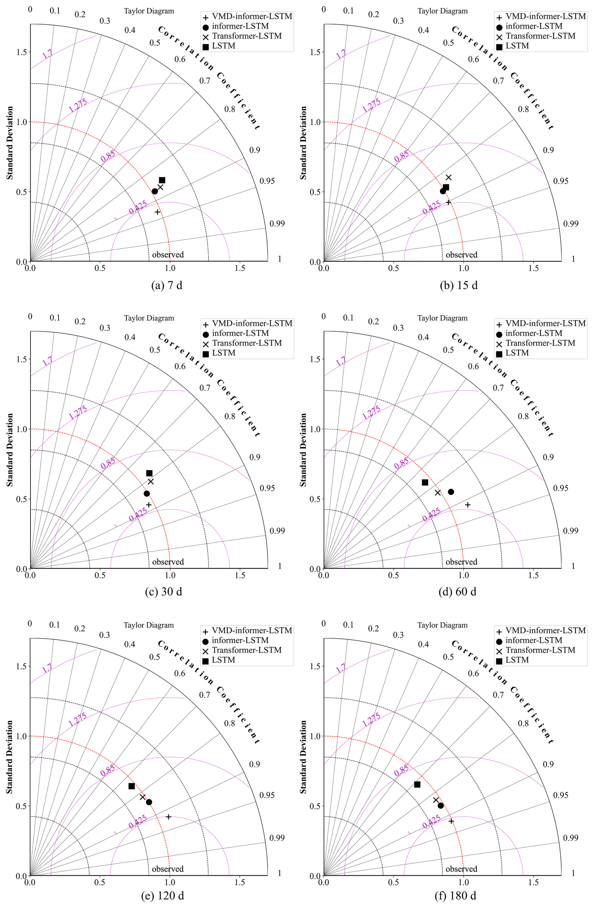
Figure 8 Taylor diagrams comparing the performance of different models for DEDI prediction in the Huaihe River Basin at different lead times: (a) 7; (b) 15; (c) 30; (d) 60; (e) 120; (f) 180 d.

4.3 Model Influencing Factor Analysis

Figure 9a presents a comprehensive SHAP value distribution analysis revealing the complex, non-linear relationships between meteorological variables and drought prediction outcomes. Precipitation emerges as the dominant predictor with predominantly positive SHAP contributions, indicating its critical role in alleviating drought conditions through direct water supply augmentation. However, the wide distribution of precipitation SHAP values (−1.00 to 2.00) suggests threshold-dependent effects, where low precipitation events contribute negatively to drought mitigation while high precipitation provides substantial positive contributions. Temperature exhibits a more complex influence pattern, with SHAP values distributed across both positive and negative domains, reflecting its dual role in drought dynamics: moderate temperatures may enhance vegetation water use efficiency (positive contribution), while extreme temperatures intensify evapotranspiration demands and soil moisture depletion (negative contribution). Figure 9b quantifies that precipitation and mean temperature collectively account for approximately 49.00 % of the total model decision-making process, with average SHAP magnitudes of 0.282 and 0.138 respectively. Surface pressure, cloud cover, and maximum temperature demonstrate moderate but consistent influences (SHAP magnitudes of 0.053 to 0.124), likely operating through indirect pathways affecting atmospheric moisture transport, radiation balance, and boundary layer dynamics. The concentrated distribution of these secondary variables' SHAP values suggests more linear, predictable relationships with drought outcomes, contrasting with the high variability observed in precipitation and temperature effects, which reflects the non-stationary nature of hydro-climatic processes and the model's capacity to capture complex feature interactions across different drought severity conditions.

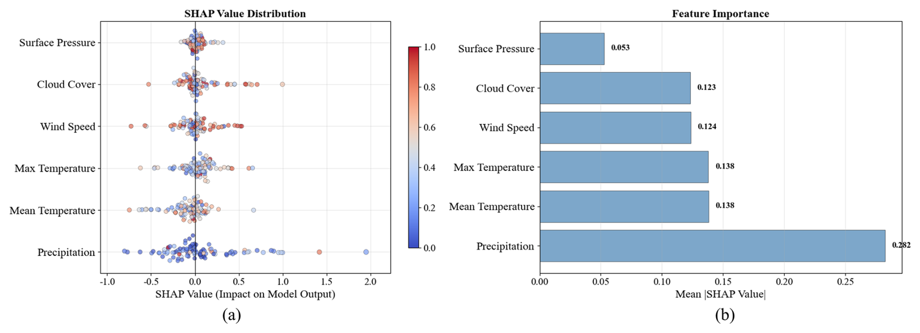
Figure 9 Relative contributions of meteorological variables to drought forecasting at a 180 d lead time.

While this study demonstrates the superior performance of the VMD-informer-LSTM model through comprehensive comparative analysis, several aspects of model uncertainty warrant acknowledgement. The concentrated performance distributions observed in violin plots suggest relatively low model uncertainty across different geographical locations, with the VMD-informer-LSTM model showing the most stable performance (IQR: 0.05 for RMSE). However, systematic uncertainty quantification through techniques such as ensemble modeling, Monte Carlo dropout, or Bayesian approaches was not implemented in this study, representing a limitation that could be addressed in future research to provide confidence intervals for predictions and better understand prediction reliability under different hydroclimatic conditions.

The spatial analysis reveals that prediction accuracy varies across the basin, with slightly higher uncertainties observed along catchment peripheries. This is potentially related to boundary effects or data quality variations. Future work should incorporate explicit uncertainty quantification methods to enhance the model's operational applicability and provide decision-makers with confidence measures alongside drought predictions.

Figure 10 illustrates the spatial prediction performance of the VMD-informer-LSTM model in the Huaihe River Basin. Overall, the model achieves the highest accuracy in the first 90 d of prediction, with an R² close to 0.92 and low error, effectively characterizing the evolution of drought. As the prediction horizon extends beyond 90 d, the accuracy shows a noticeable decline, reflecting the increasing difficulty of capturing long-term drought dynamics. In terms of spatial distribution, the upstream area performs the best, accurately reproducing the observed drought process. The downstream area follows, with the overall drought trend being tracked, though there is a tendency of underestimation in drought intensity. The midnstream area shows slightly larger errors, but maintains high consistency with ERA5 reanalysis data on a long-term scale. The Yi Shu Si River region shows a relatively balanced performance, with the model effectively reflecting changes in drought levels.

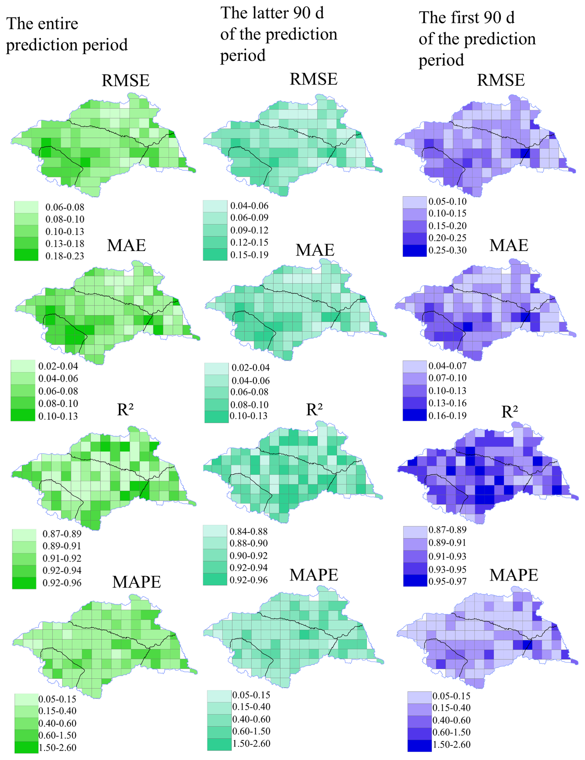
Figure 10 The spatial distribution of VMD-informer-LSTM Model performance.

Figure 11 further reveals the characteristics of drought category distribution under different prediction horizons and reflects regional differences. In the short-term predictions (first 15 d), although some models exhibit prediction errors, the overall results in the upstream, midstream, downstream, and Yi Shu Si River regions remain broadly consistent with observations. At the 7 d horizon, the LSTM misclassifies 11 grid cells, identifying the abnormally wet category as moderately wet. At 15 d, the informer-LSTM shows errors in 4 grid cells, misclassifying abnormally wet conditions as normal.

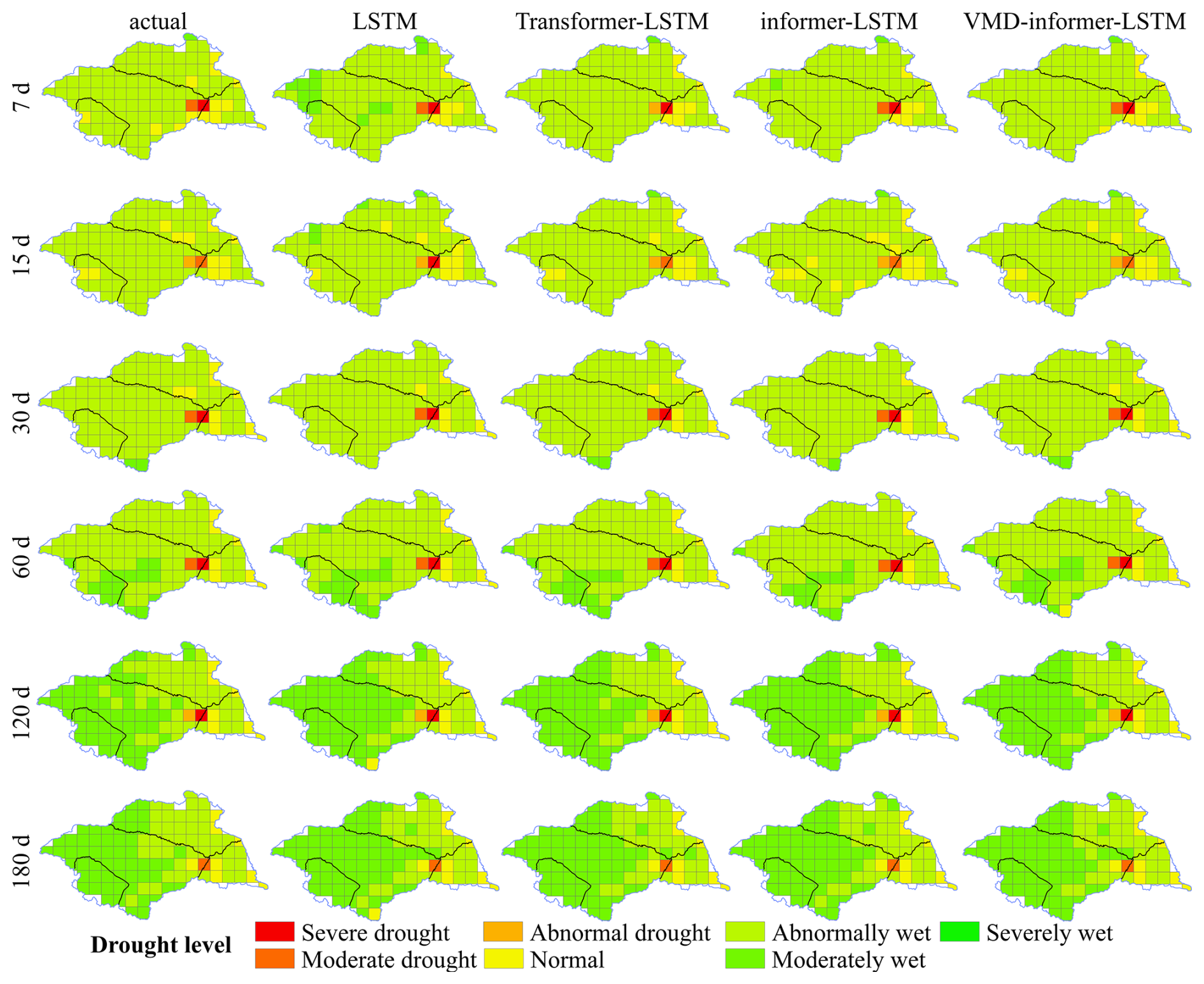
Figure 11 Comparison of drought forecasting model performance at different time scales.

In the medium-term predictions (30–60 d), the VMD-informer-LSTM demonstrates the best performance, with only 2 misclassified grid cells at both horizons, whereas the other three models show larger deviations, mainly concentrated in the upstream, midstream, and Yi Shu Si River regions. In the long-term predictions (120–180 d), prediction errors increase across all models; however, the VMD-informer-LSTM continues to maintain the highest overall accuracy. Across all prediction periods, models exhibit a common tendency to underestimate drought categories, with the VMD-informer-LSTM showing the smallest degree of underestimation.

Overall, it can be seen that the upstream and downstream regions achieved the highest observations consistency, followed by the Yi Shu Si River region, while the midstream region performed the weakest.

5 Discussion

Further combining Table 2 and Fig. 12 provides a clearer understanding of the reasons for the differences in model prediction accuracy across different regions. From 2005 to 2020, the cultivated land in the basin continuously decreased (from 187 254 to 180 161 km²), the construction land significantly increased (from 34 739 to 42 801 km²), the grassland area markedly declined, and the water area slightly increased. In the midstream region, the reduction of cultivated land, forest land, and grassland, coupled with the increase in construction land leading to the expansion of impervious surfaces, has altered the water cycle process. This has caused the model's prediction to underestimate drought severity, demonstrating that environmental changes have exacerbated hydrological droughts.

Table 2 Area of land use types in Huaihe River basin from 2005 to 2020 (km²).

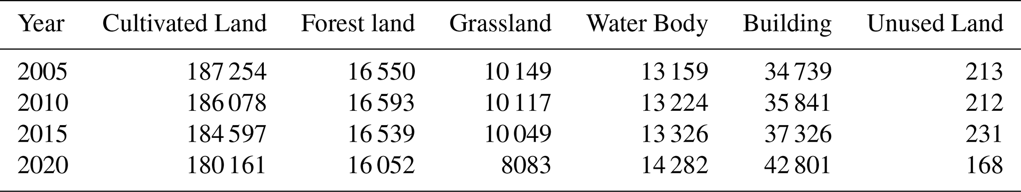
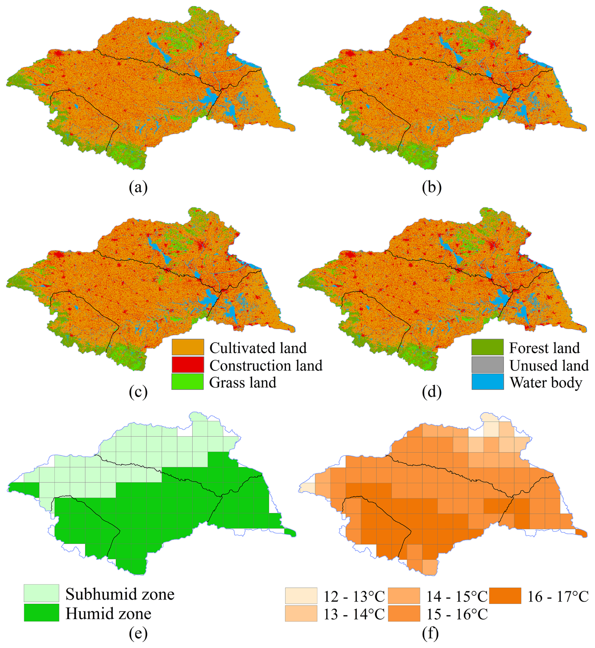
Figure 12 Distribution of Land Use, Climate Zones, and Multi-year Average Temperature in the Huaihe River Basin (a–d) Spatiotemporal distribution of land use in the Huaihe River Basin from 2005 to 2020; (e) distribution map of semi-humid and humid zones in the Huaihe River Basin; (f) distribution map of multi-year average temperature in the Huaihe River Basin.

Meanwhile, Fig. 12 shows distinct climatic zone characteristics: the upstream, southern midstream, downstream, and southern regions of the Yi Shu Si River are in the humid zone, where the annual mean temperature in the upstream and its adjacent southern midstream regions is close to 17 °C, and the annual mean temperature in the downstream and its adjacent southern midstream regions as well as the southern regions of the Yi Shu Si River is between 13–16 °C. In contrast, the northern midstream and northern regions of the Yi Shu Si River are in the semi-humid zone, with an annual mean temperature between 12 and 15 °C. Overall, the prediction results of several models underestimated hydrological drought, with misclassifications mainly concentrated in the transition zones between the humid and semi-humid regions. The semi-humid regions showed relatively more frequent errors compared to the humid regions.

The results show that the VMD-Informer-LSTM model exhibits high prediction accuracy within the 30–90 d forecast period at the time scale, while the prediction accuracy decreases during the longer forecast period of 120–180 d. Spatially, the prediction results for the upstream and downstream regions show the highest consistency with the ERA5 reanalysis values, followed by the Yishuisi River region, with the midstream region showing relatively weaker performance.In summary, the VMD-Informer-LSTM framework proposed in this study demonstrates significant advantages in handling drought index series with prominent non-stationarity and multi-time scale features, using a multi-scale modeling strategy of “decomposition – parallel modeling – feature fusion”. On the one hand, VMD effectively reduces the complexity of the original series, allowing for the separation of variation features at different time scales and modeling them individually. On the other hand, the parallel structure of Informer and LSTM focuses on capturing long-term background state changes and short-term fluctuations, enabling the model to represent both the persistence and phase-specific fluctuations of the drought process.The Huaihe River Basin is an agriculturally intensive region, where irrigation can substantially modify actual evapotranspiration and soil moisture conditions, especially during the crop growing season. Irrigation increases the water availability in croplands, enhances actual evapotranspiration, and may alleviate soil moisture deficits during dry periods. Therefore, drought prediction results in irrigated cropland areas should be interpreted with caution. Future work should incorporate spatially explicit irrigation water-use data, crop-specific water demand, ground-based soil moisture and streamflow observations, and satellite-based products such as SMAP and GRACE to further quantify and correct irrigation-related biases.

Moreover, the model is constructed using one-dimensional time series at individual grid points as input, without explicitly capturing the spatial propagation of drought, thereby neglecting the spatial interconnections among different regions. Future work will incorporate multi-source observational data and develop spatio-temporal coupling modelling approaches to enhance the representation of drought evolution processes, thereby improving the reliability of predictions.

6 Conclusion

This study takes the Huaihe River Basin in China as an example and constructs the VMD-informer-LSTM model, and compares it with the LSTM, Transformer-LSTM, and informer-LSTM models to verify its ability to predict hydrological drought in both temporal and spatial dimensions, and influencing factors are quantitatively analyzed. The main conclusions are as follows:

1. The VMD-informer-LSTM model shows clear advantages in drought forecasting across different lead times and drought severity levels. Compared with the baseline LSTM, it improves R² by 28.4 % (0.7156→0.9191) and reduces RMSE by 46.2 % (0.2087→0.1122). Further comparisons reveal that the single LSTM struggles to capture the complex drought process and performs the poorest in all models' predictions. Transformer-LSTM improves accuracy to some extent, but there is still significant error accumulation in long-term predictions. The informer-LSTM, leveraging the sparse self-attention mechanism and generative decoding approach of the informer, can balance efficiency and accuracy in long time series prediction, showing greater stability than Transformer-LSTM and being the best among the three benchmark models. However, the VMD-informer-LSTM, by introducing VMD decomposition to further extract multi-scale features and combining the long sequence modeling advantages of the informer with the local dynamic characterization ability of LSTM, achieves multi-level information fusion. Therefore, the VMD-informer-LSTM model achieves the highest precision in short-term forecasting (7 d), has the smallest error growth rate in the medium term (30–60 d), and can still more effectively characterize the evolution of drought in the long term (120–180 d). Its underestimation of drought intensity is significantly lower than other models.

2. The spatial prediction performance of the VMD informant LSTM model is influenced by land use and climate regions. Within the entire watershed, all models showed excellent prediction performance within a 30 d prediction period, with the VMD-informer-LSTM model being the most accurate. However, within a prediction period of 120–180 d, the prediction accuracy of all models significantly decreased throughout the watershed. Overall, the predicted drought intensity was relatively mild, with misclassifications mainly concentrated in the transition zones between the humid and semi-humid regions, and errors occurring more frequently in the semi-humid regions compared to the humid regions. The model performs best in the upstream region, followed by the downstream and Yishus River regions, while prediction accuracy in the midstream region is relatively weak. With the extension of the forecast lead time, this downward trend is most evident in the middle reaches, where the reduction of arable land, grassland, and forest land, as well as the expansion of construction land, have changed the water cycle process, indicating that human activities have exacerbated drought.

3. The SHAP analysis enhances the interpretability of the VMD-informer-LSTM model by revealing the relative importance of meteorological variables in drought prediction. Precipitation is the dominant factor, contributing about 28.2 % to model decisions, followed by mean temperature (13.8 %), while surface pressure, cloud cover, and maximum temperature together account for about 15 %–20 %. These results confirm that the model effectively identifies key meteorological drivers and enhances the interpretability of drought forecasting.