The influence of small farm reservoir network characteristics on their cumulative hydrological impacts

In many regions of the world, the use of infrastructure to store runoff and stream water, such as small farm reservoirs, enables irrigation and thereby secures and increases food production. The presence of multiple reservoirs in one catchment has cumulative impacts that are not necessarily the sum of the individual impacts. However, the influence of the composition and spatial configuration of a reservoir network on its hydrological impacts is still largely unknown. In this work, we investigate the influence of various characteristics of a reservoir network with a modeling approach. Our numerical experiment consists of randomly generating multiple small reservoir networks in the same catchment with realistic reservoir numbers, capacities, and spatial distributions and then comparing their hydrological impacts over a 20-year period. The catchment is representative of the agro-pedo-climatic context of southwestern France characterized by the presence of multiple small farm reservoirs for irrigating field crops. The simulations were performed using the distributed agrohydrological model MHYDAS-Small-Reservoirs, which represents small reservoirs and their links with the hydrological network and the irrigated plots. For each simulation, the impacts of reservoirs are assessed relative to a reference situation without reservoirs. To go beyond the evaluation of impacts at the outlet of the catchment solely, we developed a new indicator of low flow that summarizes the low flow experienced along the stream over a period of time. This proportion of network in low flow and the outlet discharge are computed annually and seasonally and their interannual variability is considered. In our context and with current reservoir management rules, we found that the impacts of reservoirs are more important in summer, with discharges reduced by more than 20 % and up to 60 % compared with the reference situation. Moreover, the proportion of low flow in summer is always higher than in the reference situation. The impacts vary considerably between simulations. We show that this variability can be partly explained by the characteristics of the reservoir networks. In particular, the number and distribution of reservoirs play important roles in the seasonal impacts of reservoirs. We provide an interpretation of the influence of the different factors by analyzing how reservoirs affect flows, and question the conditions under which this interpretation can be generalized to other contexts.

1 Introduction

Agricultural water management during dry periods is a common issue in many regions worldwide. Small farm reservoirs are usually considered a solution to secure water resources for irrigation during the dry season, when the availability of surface water in streams is not guaranteed and is subject to restrictions from local authorities (Carluer et al., 2017). They have been increasingly built since the 1950s in many parts of the world, such as Brazil (Pinhati et al., 2020), South Africa (Hughes and Mantel, 2010), the USA (Deitch et al., 2013), Australia (Schreider et al., 2002) and France (Galéa et al., 2005). These reservoirs can be placed directly on the stream or inserted in specific locations in the catchment to capture surface runoff and drainage waters (hill reservoirs). There are no common criteria for differentiating small reservoirs from medium or large reservoirs. Depending on the study context (e.g., location in the world or size of the study catchment), they can be defined based on a maximum surface (e.g. in Morden et al., 2022) or a maximum volume (e.g. in Ayalew et al., 2017). In this study, small reservoirs are defined as reservoirs with a capacity of less than 1 Mm³. Small reservoirs can have many uses, such as watering, flood mitigation, or groundwater recharge, but we focus on small farm reservoirs built for irrigation purposes.

Compared with other solutions for the storage of water for irrigation (e.g., storage in large reservoirs with shared use), small reservoirs are believed to have lower individual impacts on river flows and contribute to better equity between local actors in terms of water availability (van der Zaag and Gupta, 2008). However, the impacts of small farm reservoirs accumulate in a catchment along the stream (Habets et al., 2018). Thus, the impacts of a reservoir network cannot be considered as the sum of the individual impacts of each reservoir. The main cumulative impact is hydrological, i.e., stream flows are modified by the presence of reservoirs. Hydrological changes can induce other types of impacts, such as ecological, geomorphological, or biogeochemical impacts (Kennon, 1966; O'Connor, 2001; Seyedhashemi et al., 2021). These other impacts may arise not only from changes in the mean stream flow but also from variations in low flows and high flows. In agricultural catchments, low flows are usually a concern, as they can have significant effects on local and downstream stream ecology (Sarremejane et al., 2022). Many attempts have been made to assess the cumulative impacts of small farm reservoirs in different catchments around the world, and methods, especially numerical models, have been developed for this purpose (Habets et al., 2018).

The outlet discharge is the most frequently used variable to evaluate the cumulative impacts of small reservoirs (irrespective of their use). Changes in outlet discharge are often analyzed annually (e.g. Kennon, 1966; Neal et al., 2002; Hughes and Mantel, 2010; Xu et al., 2013; Yan et al., 2023) and/or monthly or seasonally (e.g. Hughes and Mantel, 2010; Fowler et al., 2015). The impacts of small farm reservoirs on floods and low flows have been less studied. In these cases, the indicators used are mostly based on outlet discharge (e.g. Galéa et al., 2005; Robertson et al., 2023; Xu et al., 2022). Few studies use spatialized approaches to characterize the impacts of reservoirs along the hydrological network (e.g. Güntner et al., 2004; Ayalew et al., 2017; Deitch et al., 2013).

Studies on the hydrological impacts of small farm reservoirs usually aim at quantifying these impacts for the current composition of the catchment in reservoirs and for the current water use (e.g. Kennon, 1966; Nathan et al., 2005; Alcorn, 2007; Deitch et al., 2013) or for some scenarios related to climate (e.g. Krol et al., 2006; Habets et al., 2014), the number of reservoirs (e.g. Meigh, 1995; Rabelo et al., 2022), their capacity (e.g. Rabelo et al., 2021), the timing and amount of withdrawals (e.g. Meigh, 1995; Brasil and Medeiros, 2020), or the filling period of reservoirs (e.g. Habets et al., 2014; Pinhati et al., 2020). However, few studies focus exclusively on understanding the factors that drive the hydrological impacts of small farm reservoirs. A better understanding is critical for land planners to determine how to minimize the impacts of existing or additional reservoirs in a catchment. The driving factors can be classified into two main categories:

• Characteristics of the reservoir network: capacity, number and spatial distribution of reservoirs.

• Management of reservoirs: filling method, link to the downstream stream, water use intensity and timing.

These factors are closely related to the pedoclimatic context and to the farming system (type of crops and type of practices). These contextual elements usually affect the development of small reservoirs in regulated catchments. A change in climate or in the farming system can trigger the construction of more reservoirs or lead to changes in their management and thereby modify their hydrological impacts.

It is well established that an increase in the total storage capacity (i.e., an increase in the reservoir size or in the number of reservoirs) associated with an increase in water use leads to a decrease in annual outlet discharge (e.g. Savadamuthu, 2002; Teoh, 2003; Thompson, 2012; Habets et al., 2014). However, its effect on other variables (e.g., low flow) remains unclear. Furthermore, the effects of the number of reservoirs with a constant capacity and the distribution of reservoirs have rarely been studied (rare examples are Ayalew et al., 2015; Meigh, 1995).

In this study, we assume that the characteristics of small reservoir networks are key factors in their cumulative hydrological impacts. Given this assumption, the objective of the study is to quantify and better understand how the cumulative hydrological impacts in a catchment are influenced by (i) the density of small reservoirs, (ii) the total capacity of the reservoirs, and (iii) the distribution of reservoirs along the stream network. To go beyond previous studies on this topic, we considered the hydrological impacts not only on mean streamflow but also on low flows. These variables were analyzed annually and seasonally. The magnitude of low flow experienced along the stream was summarized in one indicator that reflects the state of the entire network rather than solely at the outlet. As experimental or observational approaches are not feasible, we adopted a modeling approach using the spatially distributed agrohydrological model MHYDAS-Small-Reservoirs (Lebon et al., 2022). A 20-year numerical experiment was conducted for a catchment both with and without small-reservoir networks with variable characteristics. The Gélon catchment, a typical third-order catchment in southwestern France with an intermittent stream, was selected as the basis for the numerical experiment. With this approach, we were able to evaluate the effects, or influences, of the three study factors on the mean stream flow and low flow and analyze the processes driving these effects.

2 Materials and methods

2.1 The model: MHYDAS-Small-Reservoirs

2.1.1 Presentation of the model

MHYDAS-Small-Reservoirs is a spatially distributed agro-hydrological model that includes a representation of small reservoirs (Lebon et al., 2022). It is adapted for agricultural catchments that are sparsely urbanized. It is composed of a soil-crop model (Constantin et al., 2015), a groundwater model (Kirchner, 2009), a water routing model (Moussa et al., 2002), a reservoir model (Lebon et al., 2022), and a decision model for farming practices and irrigation (Murgue et al., 2014). It operates at an hourly time step for water routing and a daily time step for crop growth.

The space is described with four types of compartments: agricultural or natural surfaces, on which vegetation is growing, groundwater bodies, the hydrological network, and reservoirs. Each compartment is discretized into calculation units, which are named surface units (SUs), groundwater units (GUs), reach sections (RSs) and reservoirs (REs). Each groundwater unit corresponds to an independent groundwater body that flows directly into the hydrological network. Surface units follow parcel shapes and topography so that each unit is hydrologically linked to only one other SU, RS or RE and to one GU. Urban areas are assimilated to natural surfaces in the model, as they usually cover a small fraction of agricultural catchments. The temporal resolution is adapted to each process to be represented and thus varies from 1 h to 1 d.

An extensive description of the model can be found in Lebon et al. (2022) and Lebon (2021). In the following, we detail how reservoirs are represented in the model and how withdrawals and irrigation are addressed, as this information is essential for the experiment.

2.1.2 Representation of small reservoirs in the model

Small reservoirs are represented individually and can be directly connected to the stream network or not (hill reservoirs). They capture all upstream water and spill when they are full. A minimum flow can be fixed for each reservoir: whenever water flows upstream of the reservoir, this flow must be guaranteed downstream. Evaporation from the reservoir water is considered proportional to the reference evapotranspiration, with a coefficient of 0.6, which is a common value for this parameter also used in SWAT model applications to simulate pond evaporation (Neitsch et al., 2011). Percolation from the reservoir bed to groundwater or through the dam wall is not considered in the model, as we assume that irrigation reservoirs have impervious bed to prevent percolation. The shape of all reservoirs is the same and corresponds to a reversed half-pyramid, following the relationship reported by Liebe et al. (2005). More information on the relationship between the area and the volume is provided in the Supplement.

Small reservoirs can be unused or used for irrigation. The reservoirs used for irrigation are linked to a defined set of SUs to be irrigated. A decision model (Murgue et al., 2014) simulates the volumes of water withdrawn from reservoirs and the water applied by irrigation to the crop for each irrigated field depending on the crop demand and the availability of water in each reservoir. Additional constraints on reservoir management, such as constraints on withdrawals, can also be applied.

2.2 Numerical experiment

2.2.1 Presentation of the agro-pedo-climatic context and the support site

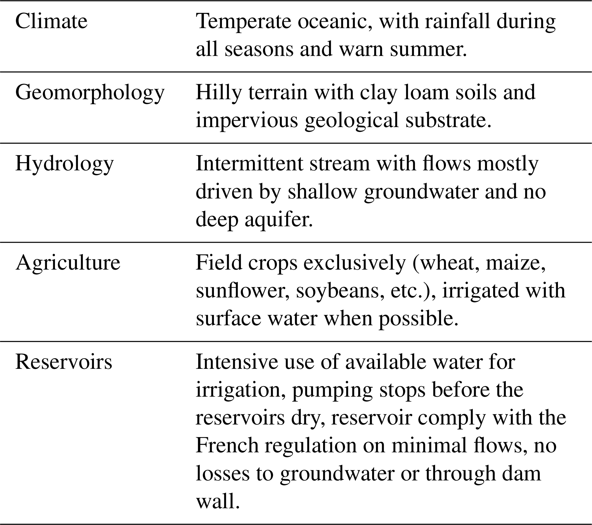
Our numerical experiment takes place in the agro-pedo-climatic context of southwestern France, a region characterized by a high density of small farm reservoirs used for irrigation. The Gélon catchment (Fig. 1) is representative of this context and was chosen as a support site for the numerical experiment. It is a 19.8 km² hilly catchment, with soils composed mainly of alluvial and molassic slope deposits (Party et al., 2016) with a clay loam texture. Soil is highly impermeable, which leads to a dense hydrological network with many irregular sources. Shallow non-perennial aquifers develop along the hillslopes and there is no deep aquifer (Cavaillé, 1968). The Gélon stream is thus intermittent. The climate is temperate without a dry season with a warm summer (Cfb, temperate oceanic) according to the Köppen-Geiger climate classification (Strohmenger et al., 2024). On average, between 2000 and 2020, annual rainfall was 650 mm, annual ET0 was 936 mm, and mean temperature was 13.6 °C. The mean monthly precipitations are equally distributed between months (always higher than 40 mm). May is the month with the highest rainfall with an average of 79 mm, and September the month with the lowest rainfall with an average of 42 mm (see the Supplement for more details). Agriculture is dominated by field crops and irrigation is a strong lever of economic development and stability for farmers (Devienne et al., 2022).

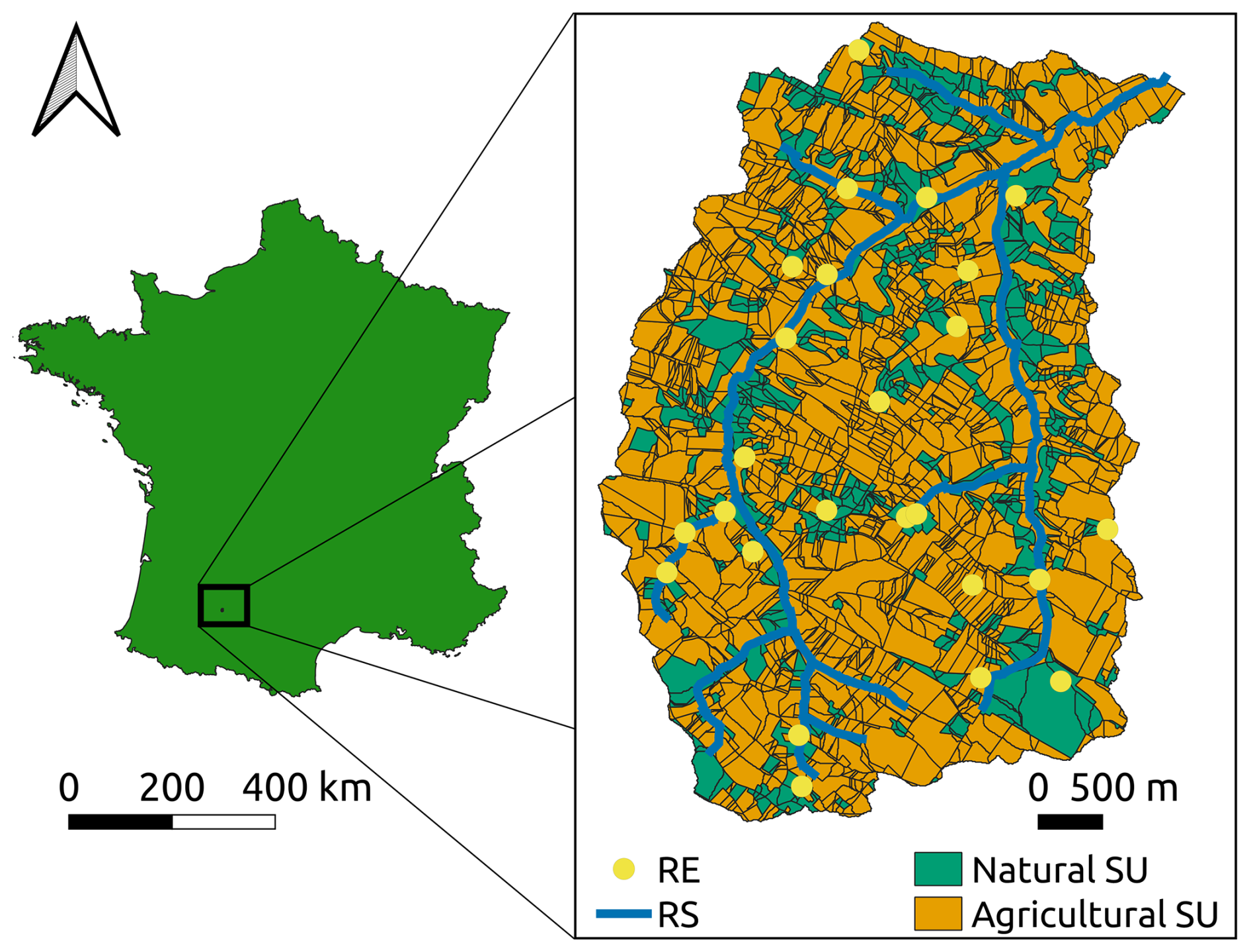
Figure 1 Localization of the Gélon catchment in France and spatial discretization in MHYDAS-Small-Reservoirs for the current network of small reservoirs.

In this context, surface water is the only available resource for irrigation. Given the high uncertainty in river flows and the possible pumping restrictions from local agencies, many farmers build their own reservoirs to store water and irrigate their crops. There are currently 25 reservoirs in the Gélon catchment (Fig. 1), with a total estimated capacity of 205 000 m³. Reservoirs located on the stream (small dams) must comply with French regulations and guaranty the transmission a minimum flow downstream whenever water flows upstream. This minimum flow corresponds to 10 % of the mean interannual discharge at the reservoir location. In southwestern France, farmers usually stop pumping in reservoirs before they dry to preserve the pumping material and ensure the quality of the irrigation water.

2.2.2 Model instantiation for the support site

In the numerical experiment, the field layout, stream network and ratio of agricultural land to noncultivated land at the support site correspond to real-world conditions and are represented in the model as specified in Lebon et al. (2022). Thus, the Gélon catchment is divided in the model into 2402 SUs, representing approximately 15 km² of agricultural land and 5 km² of noncultivated land. The 8 km long hydrological network is divided into 365 RSs (Fig. 1).

MHYDAS-Small-Reservoirs was previously applied, calibrated and validated on the Gélon catchment for the hydrological year 2014/15 to evaluate the impacts of the existing reservoirs (Lebon et al., 2022). Compared with the previous use of the model on the Gélon catchment (Lebon et al. (2022)), the number of groundwater units was increased from 17 to 282 to better fit the field observations. This adjustment did not considerably modify the flows at the outlet, but the new groundwater units better represent a continuous water supply from shallow hill aquifers along the hydrological network.

In this work, we were not interested in the hydrological impacts of current reservoirs. The catchment served as a basis on which the model accurately represented the processes related to water flows and crop growth and management in the agro-pedo-climatic context of southwestern France (summarized in Table 1), and we used the model with hypothetical numbers, positions, and characteristics of reservoirs. Two assumptions are made for the management of these hypothetical reservoirs: (i) they comply with the French regulation on minimum flows, and (ii) there is no restriction on annual withdrawals, but there is a threshold volume below which withdrawals are not allowed to represent this common practice. We set this threshold at $\mathrm{1}/\mathrm{4}$ of the reservoir's capacity (as in Lardy et al., 2016).

Table 1 Summary of the agro-pedo-climatic context of the study.

2.2.3 Approach

The numerical experiment involved generating multiple situations, each corresponding to a different reservoir network in the same catchment. Each network had a different reservoir density, total capacity, or spatial distribution. Under real conditions, the irrigated fields are located close to the small reservoir used for irrigation. Therefore, for each generated reservoir network, we also determined a specific spatial allocation of irrigated crops that corresponded to a predefined statistical distribution of irrigated crops in the catchment.

For each study factor, different modalities were chosen prior to the experiment: three for the number of reservoirs, two for total stored capacity in the catchment, and three for the random placement of reservoirs on the hydrological network. Each combination of modalities is repeated 5 times, leading to a total of $\mathrm{3}\times \mathrm{2}\times \mathrm{3}\times \mathrm{5}=\mathrm{90}$ situations.

With this approach, two situations have:

• Different or equal numbers of reservoirs depending on the chosen value.

• Different or equal reservoir capacities depending on the chosen values for the total stored capacity and the number of reservoirs.

• Different positions of reservoirs in the hydrological network. Depending on the chosen method, there are more reservoirs upstream, downstream, or they are more equally distributed.

• Different irrigable parcels depending on the placement of reservoirs. The crops on these parcels are different from those in the reference situation. For a parcel selected in two situations, the associated irrigable crop can be different.

• Equal total surface area of irrigable land and equal total surface area of each irrigable crop.

For each network, a simulation was performed with the MHYDAS-Small-Reservoirs model. In addition, a simulation without any reservoir or irrigation was performed to serve as the reference situation. The hydrological impact of each generated reservoir network was quantified as the difference between the simulation with that network and the reference situation. The situations with reservoirs are designated “impacted situations”.

In the following sections, we describe the choice of values for the study factors and the distribution of irrigated crops (Sect. 2.2.4), and the method to generate each of the 90 reservoir networks with a random allocation of irrigable crops near reservoirs (Sect. 2.2.5). Finally, we detail the setup of the simulations in Sect. 2.2.6 (simulation period, initialization, and crop and weather data).

2.2.4 Values for the study factors

Three values were chosen for the total number of reservoirs: 7, 14, and 21. They correspond to densities of approximately 0.35, 0.70, and 1.06 km⁻², as these values are quite representative of this region (DDT82, 2022). To determine the distribution of reservoirs along the stream, three methods were designed. They are designated “upstream”, “balanced”, and “downstream” and are described in more detail in Sect. 2.2.5. As hill reservoirs are usually found in locations where surface and subsurface flow converge, which is not captured by the model, a random placement would not be meaningful for this type of reservoir. Therefore, the reservoirs are placed only on the hydrological network in the experiment. The total stored volume was fixed along with the total irrigable area and the distribution of irrigable crops. The distribution of irrigable crops was calculated from regional data (i.e. Pignard et al., 2023). The main irrigable crops are maize, straw cereals, and soybeans (Table 2).

Table 2 Distribution of irrigable crops used in the numerical experiment, mean irrigation water use, and irrigation period for these crops. The distribution is calculated from regional data, and the mean irrigation water use is evaluated with the model with simulations performed over the study period with a single parcel and a single crop without limitations on water availability.

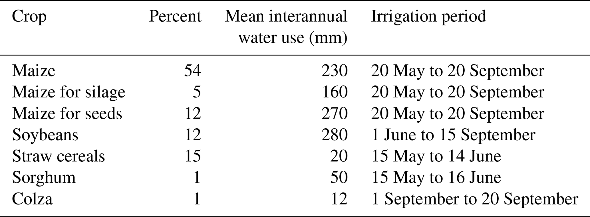
The total irrigable area is fixed so that the mean water use for irrigation without limitations represents 5 % of the mean annual naturalized flow determined in the reference situation. The mean water use was estimated with the crop model (i.e. AqYield, Constantin et al., 2015) for each crop individually (Table 2). This estimation led to a surface of approximately 1 km² (the value of 1 km² was retained) and an annual water need of 210 000 m³. Considering that only $\mathrm{3}/\mathrm{4}$ of the water stocks in reservoirs can be used for irrigation (see Sect. 2.1.2), this situation led to a value of 280 000 m³ for the storage capacity. The value of 280 000 m³ thus corresponds to a situation where the total stock in reservoirs at the beginning of the cropping season is sufficient to cover the irrigation demand in average years. The second value tested for the total capacity was fixed to 140 000 m³, representing a situation where water stored in reservoirs in winter alone will probably not be sufficient to cover all the water demand. The chosen values were determined to be reasonable considering the current estimated storage of approximately 205 000 m³ distributed into 25 small reservoirs in the Gélon catchment.

2.2.5 Creation of the reservoir networks

The generation of each reservoir network requires four steps. They are presented in Fig. 2 and described below. The starting point is the catchment in the reference situation without reservoirs (Step 1 in Fig. 2). The placement of small reservoirs on the hydrological network consists of selecting a set of RSs on which the chosen number of reservoirs will be placed. For this purpose, the 365 RSs that make up the hydrological network in the numerical representation of the catchment are divided into two subsets: upstream and downstream. The criterion used to separate the two subsets is a threshold of the drained area. This threshold corresponds to the maximum drained area of first-order streams (approximately 2.5 km²). Since RSs have different lengths, it is useful to compare the sizes of the subsets by their total lengths. A total of 55 % and 45 % of the total network length are included in the upstream and downstream subsets, respectively (see the Supplement for more information). The placement of a reservoir on the network is carried out with two consecutive random draws. In the first draw, one of the subsets is selected, and in the second draw, one of the RSs of the selected subset is chosen. In the first draw, the probability associated with each subset depends on the selected method. For the methods “upstream”, “balanced”, and “downstream”, the probabilities of drawing the upstream subset are 0.8, 0.5, and 0.2, respectively. In the second draw, the selection of each RS of the selected subset is equiprobable.

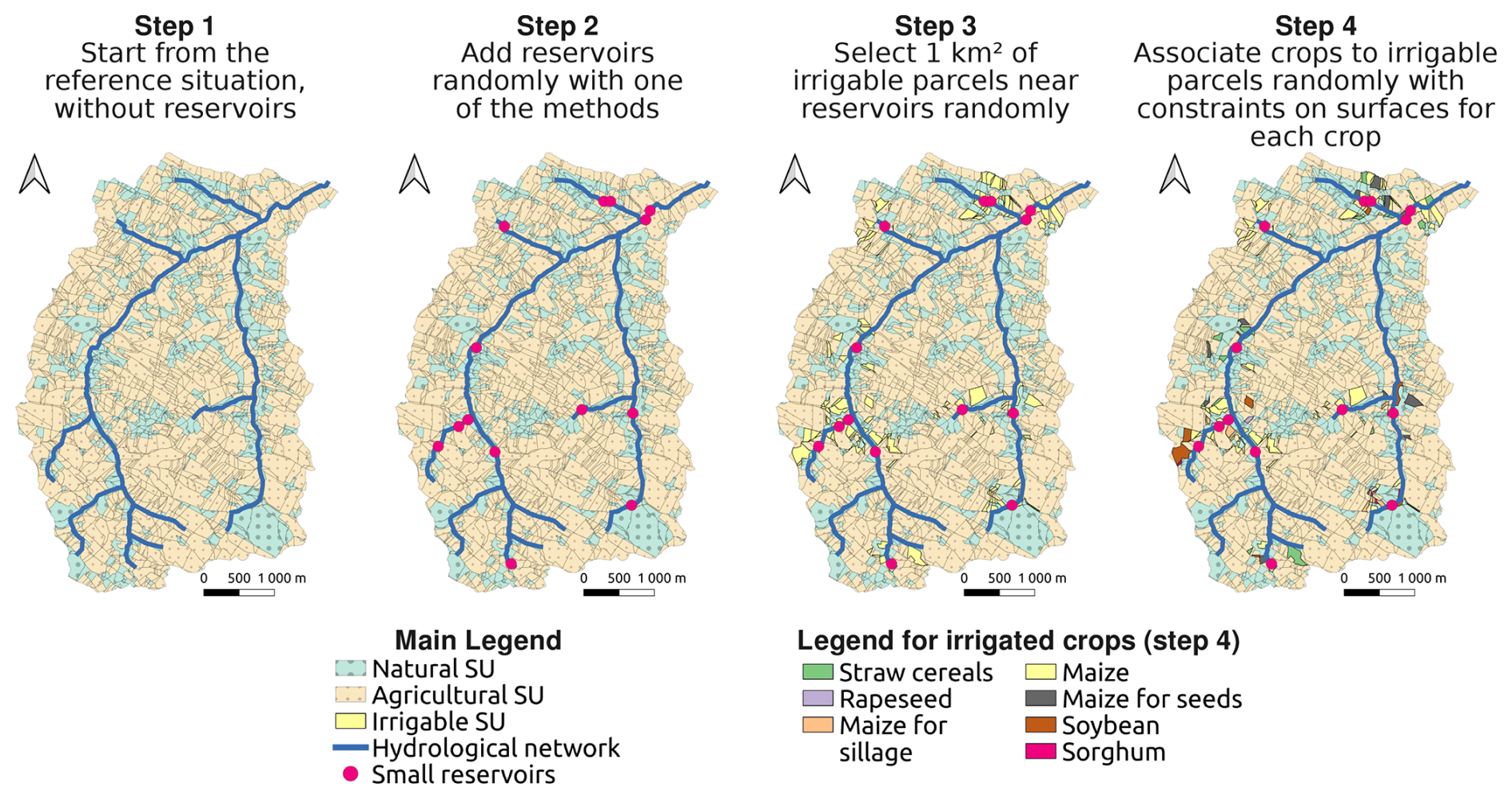
Figure 2 The 4 steps to generate a reservoir network and the subsequent changes in the catchment prior to simulation. The 14-reservoirs network is generated with the “upstream” method.

Once a location is selected for each reservoir, the hydrological network is modified to include the new reservoirs (Step 2 in Fig. 2). The total storage capacity is evenly distributed across all the reservoirs, and the area of the neighboring SU is reduced to consider the spatial extent of the reservoirs. More information on the considered shape for reservoirs and the subsequent area-to-volume relationship, along with an example of reservoirs distribution obtained with each of the three methods, can be found in the Supplement.

After the reservoirs are placed on the hydrological network, the allocation of crops is carried out in two steps. First, a set of SUs is randomly selected near each RE (within a distance of 1000 m) to reach a total of 1 km² of irrigable land in the catchment that is evenly distributed between all the reservoirs (Step 3 in Fig. 2). A tolerance threshold of 1 % is applied to the value of 1 km² to address the different parcel sizes. An irrigable crop is subsequently associated with each of the selected parcels. The irrigable crops are chosen among the predefined set (Table 2), and the distribution between the available parcels is determined to have the same distribution of irrigable crops at the catchment level in all 90 situations with a tolerance threshold of 2 % (Step 4 in Fig. 2).

2.2.6 Setup of simulations

The 90+1 simulations are run from 1 September 1995 to 1 January 2021. The parameterization of the model is the same as that in Lebon et al. (2022). Since the initial conditions cannot be determined, we use a warm-up period instead. Lebon (2021) reported that for the application of the MHYDAS-Small-Reservoirs to the Gélon catchment, a warm-up period between 2 and 5 years was sufficient to reach satisfactory initial conditions. Here, we consider a 5-year warm-up period. These five years are not included in the analysis. Therefore, the analysis can start in September 2000.

Each agricultural SU is associated with a crop. Although the model can support crop succession, only one crop was associated with each SU for all the simulated years, corresponding to the main crop of the 2014–2015 cropping season, which is available in the French Land Parcel Identification System (IGN, 2015). Thus, each year can be seen as the repetition of the same agricultural year with varying initial conditions and weather.

The weather data are composed of hourly SAFRAN data for rainfall and temperature, and daily data for the minimum daily temperature and reference evapotranspiration (Penman-Monteith). The SAFRAN climatic data are provided by Météo-France and were downloaded via the SICLIMA platform developed by AgroClim-INRAE. The data are reanalysis of observed data on 8 km×8 km cells (Bertuzzi et al., 2022; Vidal et al., 2010). The Gélon catchment intersects with 2 of these cells. One of these two covers more than 97 % of the catchment area. The seasonal rainfall for the main cell is presented in Fig. 3.

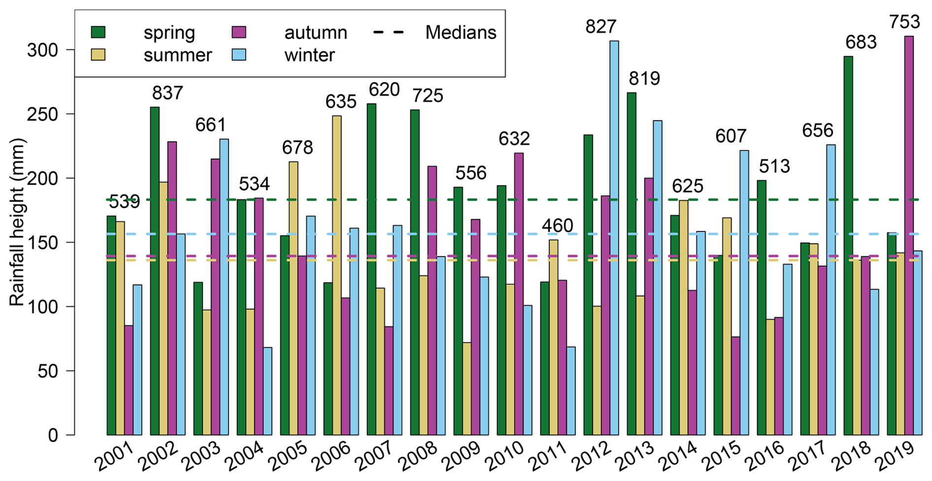
Figure 3 Seasonal rainfall during the study period for SAFRAN cell 8558. Years start in spring (on 1 April). The yearly rainfall height in mm is indicated on top of the bars for each year.

2.3 Method of analysis

2.3.1 Indicators of impact

To analyze and compare 90+1 simulations, synthetic indicators are needed. In this study, 2 indicators were chosen: the outlet discharge and the proportion of the network in low flow. The outlet discharge is commonly reported in the literature. It is also easy to compute and compare between simulations. However, it provides information only on what happens at the outlet and not on the remaining hydrological network.

The proportion of the network in low flow is a new indicator developed in this study to provide information on flow that is spatially aggregated. Each day, the total length of the network in low flow is computed by comparing the discharge in each RS with a local low flow threshold. Afterward, the mean proportion of the network in low flow during the study period (a year, a season, a month) can be computed.

The daily discharges on the 365 RS in the reference situation are used to compute these low flow thresholds for each RS. They correspond to the Q₉₀, the discharge that is exceeded 90 % of the time, computed during the study period.

Both the daily outlet discharge and the proportion of the network in low flow are outputs of the model. They are further aggregated for analysis.

2.3.2 Seasonal and annual aggregation

The results are analyzed on a yearly and seasonal basis. The years of analysis span 1 April of year N to 31 March of year N+1. Thus, the impacts of reservoirs are studied for a period in which they are first emptied in spring and summer and then filled the remainder of the year to reach their maximum capacity at the beginning of each year. This was effectively observed for nearly every year and situation (see Sect. 3.4.2). In the Results section, the seasons are therefore displayed in the following order: spring (civil year N), summer (N), autumn (N), and winter (N+1). The simulation results are thus analyzed from 1 April 2001 to 31 March 2020, which constitutes a total of 19 years.

2.3.3 Identification of the most influential factors

The effects of the studied factors, namely the total storage capacity, density and spatial distribution of reservoirs, are analyzed in terms of direction and magnitude. The direction is derived from boxplots performed for each factor studied. The magnitude is assessed using a decomposition of variance with a linear model (ANOVA), including interaction terms. With this method, the different factors can be ranked according to their relative contributions to the observed variance. As there is high interannual variability in climate forcing (see Fig. 3), the results are presented year by year.

3 Results

3.1 The proportion of network in low flow

In this study, we use a new indicator to assess the impacts of small reservoirs on low flows (Sect. 2.3.1). Figure 4 illustrates how the indicator value relates to the number of low-flow days along the stream. Situations with longer portions of networks presenting higher number of low-flow days during the aggregation period will be associated with higher low-flow proportions.

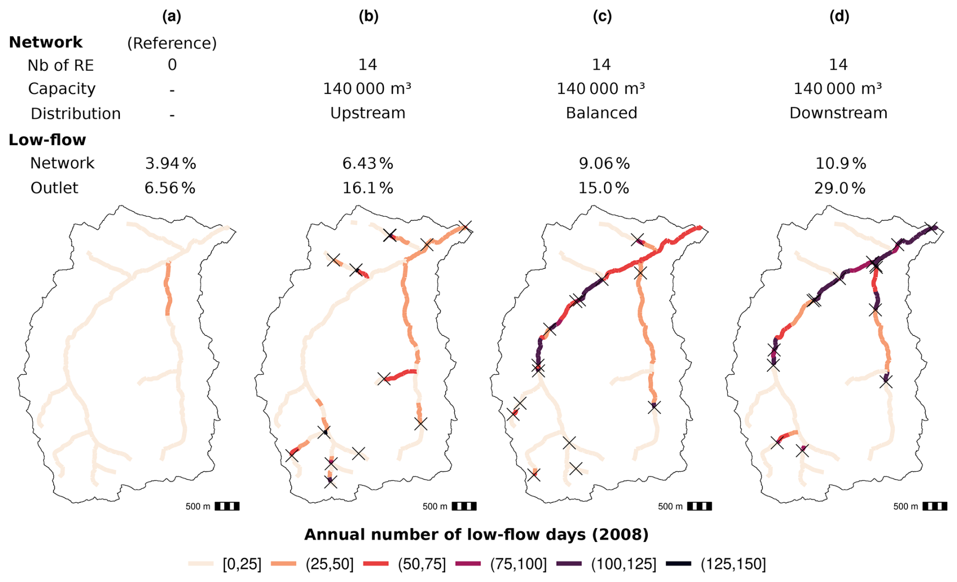
Figure 4 Maps of the number of low-flow days on each portion of the hydrological network for the year 2008 for the reference situation without reservoirs (a) and for 3 situations at 140 000 m³ of total capacity, 14 small reservoirs, obtained with the upstream (b), balanced (c), and downstream (d) method. 2 indicators of low-flow are presented on top of each plot: the proportion of network in low flow, and the proportion of time with low flow at the outlet (number of low-flow days normalized by the number of days in the year).

For the year 2008, there is almost no low-flow in the reference situation (Fig. 4a). The low-flow proportion increases in situations with reservoirs, with differences between the three presented situations (Fig. 4b–d). The portions of the network experiencing low-flow and the number of low-flow days vary depending on the distribution of reservoirs. The distance of impact of upstream reservoirs located on different branches of the hydrological network is usually low (Fig. 4b and c). When multiple reservoirs are located on the main section of the hydrological network, the whole section is impacted (Fig. 4c and d).

This spatial approach reveals interesting relationships between reservoir location and low-flow location and severity. However, it cannot be used to study low flows in the 90 simulation and for the 19 years of analysis and was not further developed in this study. As shown in Fig. 4, the new indicator of low flow is able to summarize the information on the number of low-flow days experienced along the stream. Compared with the number of low-flow days at the outlet, it can distinguish the four spatially different situations presented. That is because the number of low-flow days at the outlet is particularly sensitive to the presence of a reservoir near the outlet, as is the case in Fig. 4.

3.2 Quantification of reservoir impacts

3.2.1 Annual impacts

Simulated annual outlet discharges in the reference situation (without reservoirs) show large interannual variability, with values ranging from 80 to 400 mm (e.g., from 1.6×10⁶ to 8×10⁶ m³). As expected, the outlet discharge is always lower in the impacted situation than in the reference situation (Fig. 5a). However, relative to the reference situation, the decreases in outlet discharge are small, and the variability between situations for a given year is quite small, especially compared with the interannual variability in discharge. Absolute decreases in annual outlet discharge are usually between 4 and 9 mm (Fig. 9), which represents between 1 % and 6 % of the annual outlet discharge in the reference situation, except in 2011 and 2016, when it represents between 5 % and 15 % of the annual outlet discharge. These two years are the years with the lowest total rainfall (Fig. 3).

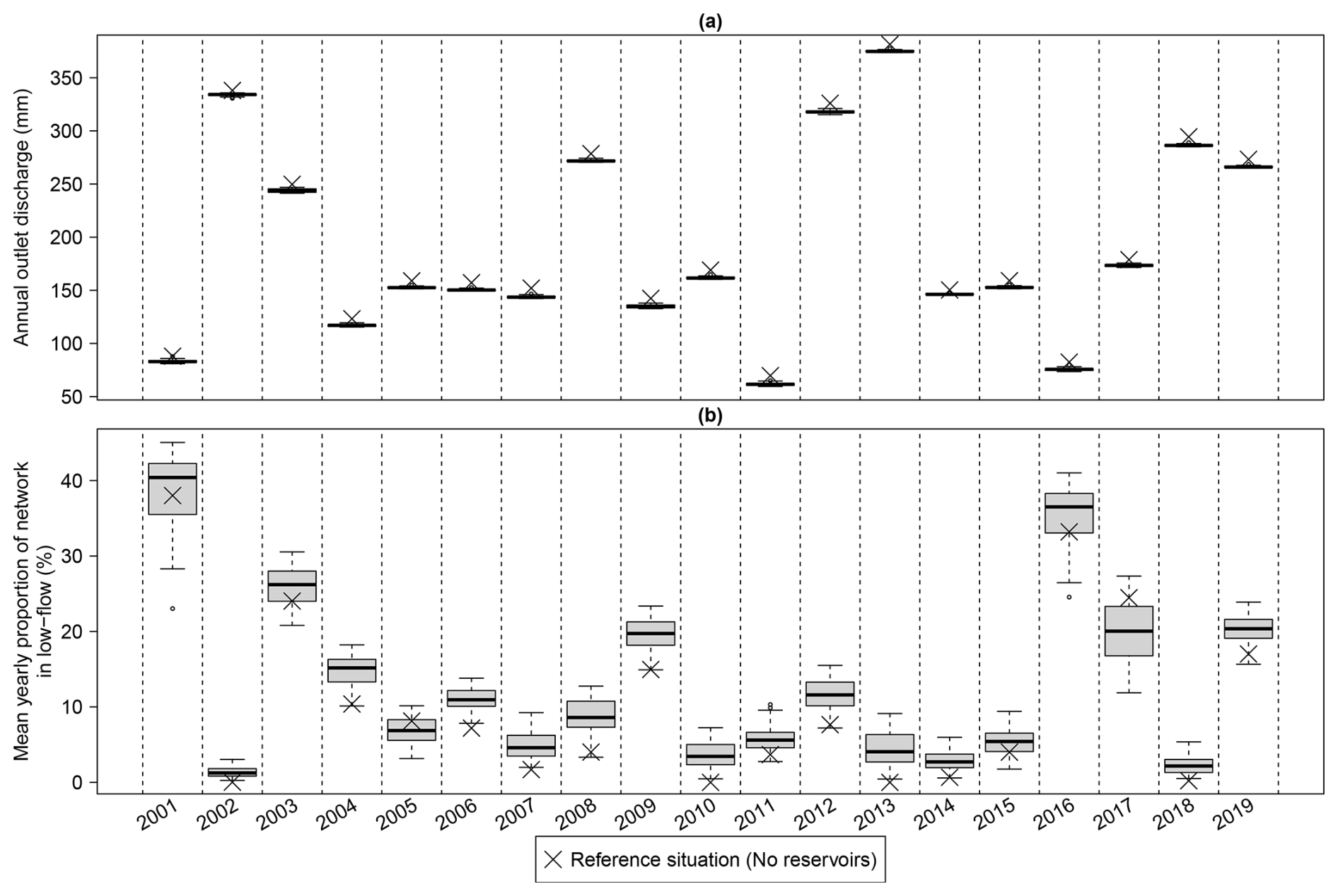
Figure 5 Boxplot of annual outlet discharges (a) and annual proportions of the network in low flow (b) in the 90 situations for the simulated years. × represents the values in the reference situation. The years analyzed span April n to March n+1.

Compared with the annual outlet discharge, the impacts of reservoirs on the annual proportion of the network in low flow exhibit high variability between the simulations (Fig. 5b). Depending on the year and the situation, the proportion of the network in low flow can increase or decrease compared with the reference. For years with low proportions of the network in low flow in the reference situation (i.e., <20 %), reservoirs usually increase this proportion. In particular, in years with no low flow in the reference situation, such as 2010 or 2013, the proportion of the network in low flow can reach 10 % in impacted situations. For years with high low flow proportions in the reference situation (i.e., >20 %), the effect of reservoirs on low flow can be positive or negative depending on the situation. For these years, the variability between the impacted situations is usually higher.

3.2.2 Seasonal impacts

The impact of reservoirs on outlet discharge is more important in summer in both relative and absolute terms (Fig. 6a). The summer decreases in outlet discharge are consistently higher than 2 mm and can reach 10 mm, with most values in the 3–7 mm range. In relative terms, this range represents between 20 % and 60 % of the summer discharge in the reference situation (Fig. 6b). In the other seasons, the discharge usually decreases compared with the reference situation, but there are also some years and some situations for which it increases, especially in autumn. In autumn, years with increases or decreases in the outlet discharge in the impacted situations are usually the same for all simulations, which shows that the weather is a determining factor of reservoir impacts. For example, 2001, 2002, 2005, 2006, 2011, 2014, 2015 and 2017 are the years in which the autumnal outlet discharge increased, and the summer rainfall of all these years is higher than the median value during that period (Fig. 3).

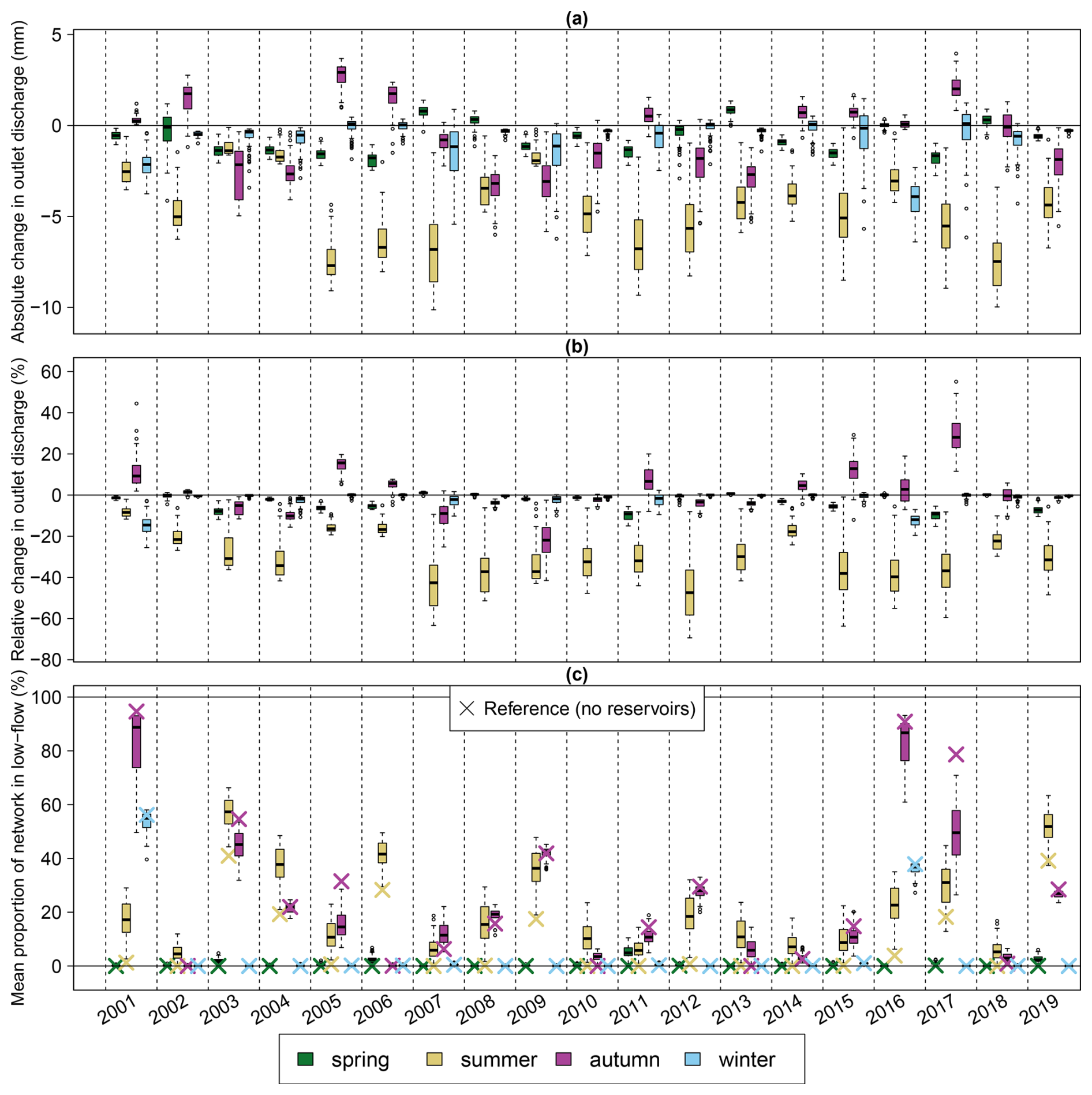
Figure 6 Boxplot of absolute (a) and relative (b) changes in the seasonal outlet discharge and boxplot of the seasonal low flow proportion (c) for the simulated years and the 90 impacted situations compared with the reference situation.

In all situations, most of the low flow occurs in summer and in autumn (Fig. 6c). In the reference situation, there is no low flow in spring and winter, except for the years 2002 and 2017, when low flow lasts until winter. In spring, the proportion of the network in low flow remains low for all years in the impacted situations (except in 2011). In summer, the low-flow proportion increases in all the impacted situations, generally by at least 5 % and up to 30 % (in absolute terms). In autumn, the effect of reservoirs depends on the year. Compared with the reference, the proportion of the network in low flow can either increase or decrease, but for most years, it tends in the same direction for all the impacted situations. Except for some years (especially 2001, 2016 and 2017), the variability between the impact situations is lower than that in summer. For years with a high proportion of the network in low flow in autumn in the reference situation (>20 %), the presence of small reservoirs always decreases the proportion. In the winter, the proportion of the network in low flow in the impacted situations is usually close to 0. For the two years with extended low flow in winter, the proportion decreases slightly in the impacted situations. In summary, compared with the reference situation, small reservoirs generally (i) increase the annual proportion of the network in low flow (Fig. 5b) and (ii) modify the low flow period, which starts earlier, in spring or summer, and can also end earlier in autumn.

3.3 Effect of the study factors

To analyze the effects on the hydrological impacts of the different factors, we focus on the indicators for which the impact of the reservoirs is the most important and variable. The five indicators we selected are (i) the annual outlet discharge, (ii) the summer outlet discharge, (iii) the annual proportion of the network in low flow, (iv) the summer proportion of the network in low flow, and (v) the autumnal proportion of the network in low flow. This analysis is presented in two subsections, each corresponding to a different step. First, we analyze in which directions these factors affect the indicators, i.e., whether the factors have a positive or negative impact. Second, we quantify the relative contribution of the three factors to the impact on the indicators. The effect, or influence, of each factor is therefore analyzed in terms of direction and magnitude. The main outcomes of this analysis are summarized in Table 3.

Table 3 Summary table of the simulated effects of the three study factors on five indicators of impacts in our studied context. The first line indicates the global effect (indicator increase ↗ and decrease ↘). The other lines indicate the effect and the mean order of importance of each factor in the ANOVA (indicated by the number in brackets). Empty cases indicates that the factor has no impact on the indicator. Low flow refers to the indicator of the proportion of the network in low flow. An increase in low flow is perceived as a negative impact. For the autumnal low flow, only years with more than 20 % of low flow in the reference situation were retained to address the variability in the ANOVA.

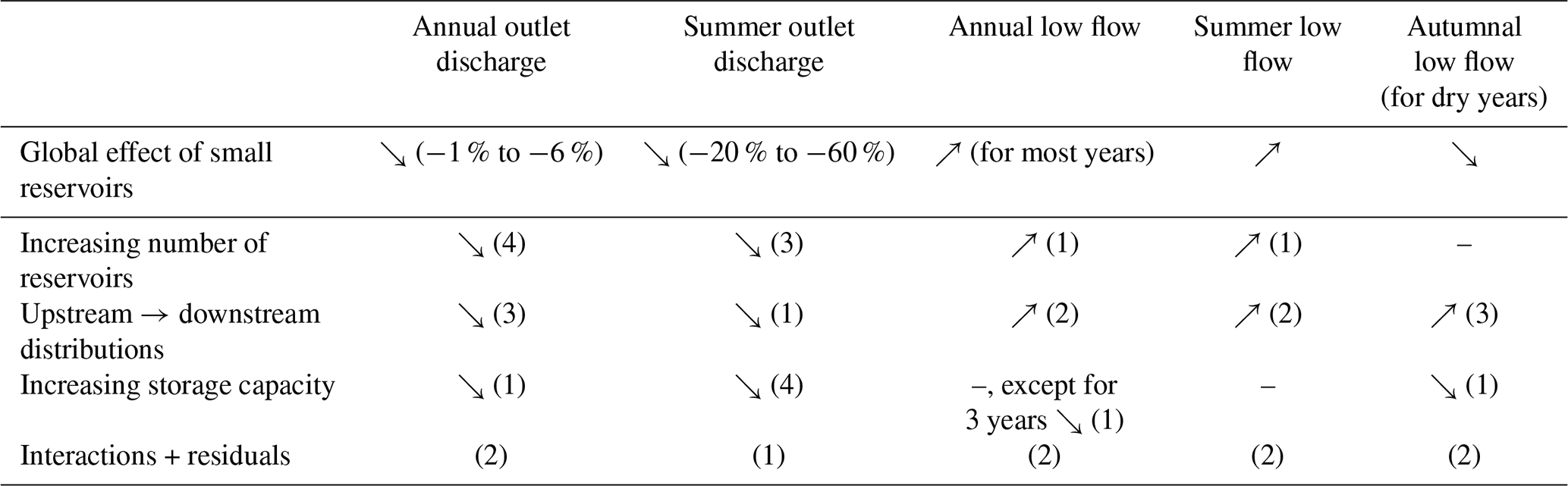
3.3.1 Directions of the effects

Among the five indicators, the storage capacity consistently influences the annual and summer outlet discharge (Fig. 7a and d respectively). In both cases, increased capacity leads to higher impacts. The effect on annual discharge is clearer than that on summer discharge (each year, the intersection between boxes is systematically smaller in (a) than in (d)). For most years, the effect of storage capacity on low flow is unclear. With respect to the annual proportion of the network in low flow, the storage capacity is relevant only in 2001, 2016, and 2017, which were all particularly dry years in terms of rainfall, especially in autumn. In general, higher storage capacities seem to be associated with lower annual proportions of the network in low flow, but this observation does not hold for all years, and the effect is usually small. In summer, the storage capacity has no effect on low flow, except in 2017. The summer of 2017 is close to the median in terms of rainfall but follows a succession of four dry seasons after the summer of 2016. Situations with 280 000 m³ of storage capacity are associated with less summer low flow than situations with 140 000 m³ of storage capacity but still more than in the reference situation. Finally, in autumn, the storage capacity has an influence in 2001, 2003, 2008, 2009, 2012, 2016, 2017, and 2019. For these years, increased storage capacity leads to lower proportions of the network in low flow.

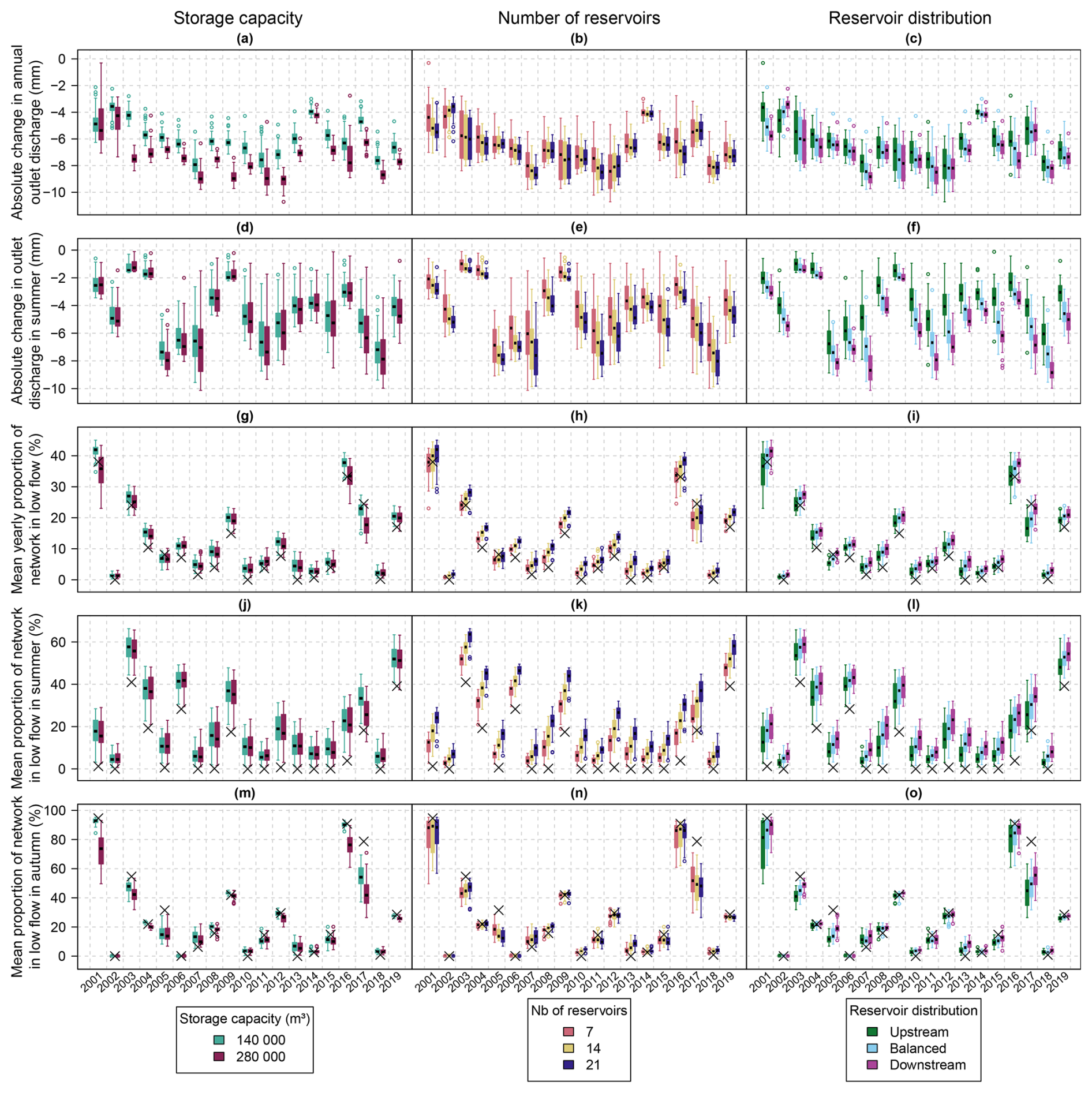
Figure 7 Boxplot each of the five indicators of impact (rows) for each simulated year, separating the effect of each factor (columns). The indicators of impact are the absolute change in the annual outlet discharge (a–c), the absolute change in the summer outlet discharge (d–f), the mean annual proportion of the network in low flow (g–i), and the mean proportions of the network in low flow in summer (j–l) and in autumn (m–o). For the proportions of the network in low flow, the large crosses indicate the values in the reference situation.

The number of reservoirs consistently affects nearly all the indicators (Fig. 7 middle). Only its effect on the autumnal proportion of the network in low flow is inconsistent across years. In general, increasing numbers of reservoirs are associated with higher impacts, i.e., greater decreases in annual and summer outlet discharges and proportions of the network with low flow. With respect to the autumnal proportion of low flow, the effect of the number of reservoirs can occur in either direction depending on the year.

When reservoirs are located more downstream, their hydrological impacts increase, i.e., lower annual and summer discharges at the outlet and higher proportions of the network in low flow throughout the year (Fig. 7 right). The only exception occurs in 2002. For this year only, higher numbers of reservoirs and reservoirs located downstream are both associated with lower decreases in annual discharge at the outlet. This finding could be related to the succession of a rainy spring, summer, and autumn in that year.

3.3.2 Relative contribution of factors

The boxplots in Fig. 7 show that some factors have a stronger effect than others do on the study variables. Figure 8 shows the relative contribution of each factor to the variability of each indicator for each year, according to an analysis of variance. A quick review reveals that (i) the main explanatory factor is different for each indicator (i.e., different main colors on each plot), (ii) for a given indicator, the main explanatory factor can be quite different from year to year (i.e., different color distributions from year to year), and (iii) the residuals of the ANOVAs, i.e., the proportion of variance that is not explained by the study factors, are high for all indicators (i.e., the sky blue color is consistently present throughout the figure).

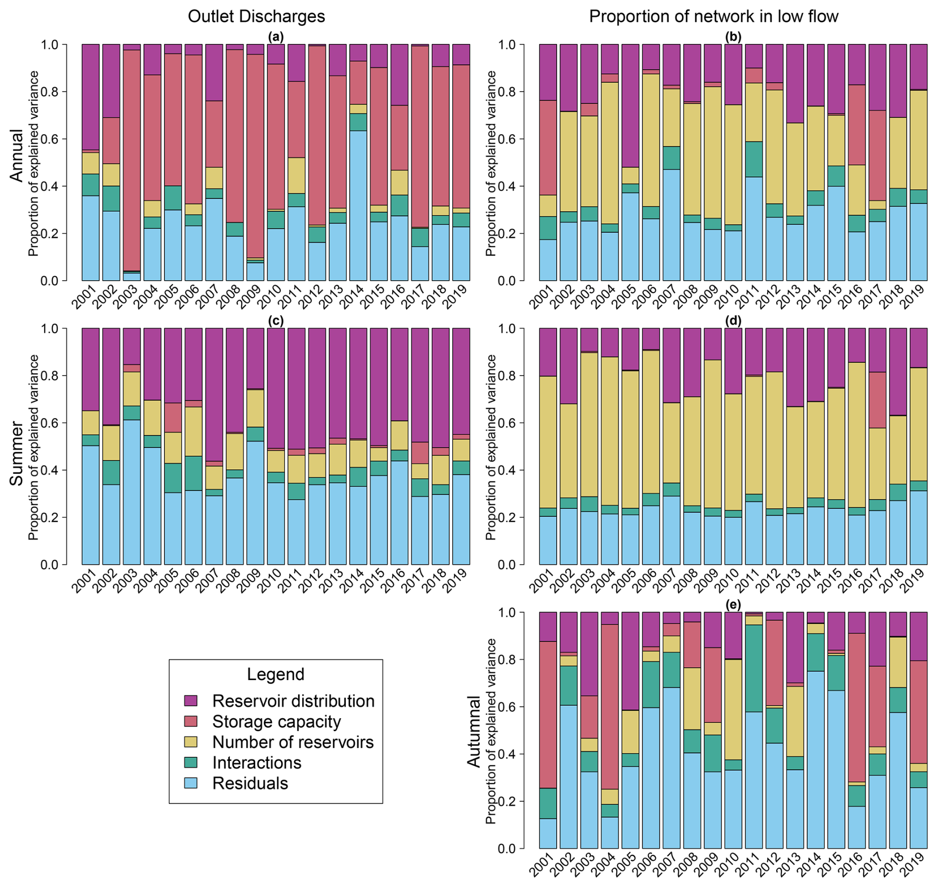
Figure 8 Decomposition of the observed variance in the impact situations for each year and for 5 variables: annual outlet discharge (a), annual proportion of the network in low flow (b), summer outlet discharge (c), and summer (d) and autumnal (e) proportions of the network in low flow. The decompositions of variance are performed with an ANOVA with three explanatory factors and their interactions: reservoir distribution, total storage capacity, and number of reservoirs. The years analyzed span April n to March n+1.

Storage capacity is the most important factor for explaining the variability in annual outlet discharge, but it has only a limited effect on the variability in summer discharge. For the proportion of the network in low flow, its effect differs depending on the year. In autumn, its contribution to the variance is important in 2001, 2003, 2004, 2008, 2009, 2012, 2016, 2017, and 2019, which corresponds to years with more than 20 % autumnal low flow in the reference situation. In 2001, 2016 and 2017, the storage capacity makes an important contribution to the annual proportion of the network in low flow, corresponding to the three years with the most autumnal low flow in the reference situation. Finally, the storage capacity has a substantial effect on the proportion of low flow in summer only in 2017; it has no effect in the other years.

In most years, the number of reservoirs is clearly the main explanatory factor for the annual and summer proportions of the network in low flow and is consistently followed by the distribution of the reservoirs. The opposite is true for the summer outlet discharge: the distribution of reservoirs is the main explanatory factor, followed by the number of reservoirs. Both factors contribute little and inconsistently to the variance in the annual outlet discharge.

The decompositions of variance for the autumnal proportions of the network in low flow are more difficult to analyze, as the contributions of each factor change every year. If we consider the years with the highest proportions of the network in low flow in autumn (i.e., more than 20 %), the storage capacity is consistently the main factor, the distribution of the reservoirs is a secondary contributor, and the number of reservoirs has little to no effect.

For all the indicators, the residuals and interaction terms are high and variable from year to year, which means that an important proportion of the variance is not easily explained by our factors (i.e., by a linear model of the modalities of our factors). The indicator with the consistently lowest residuals and interactions is the summer proportion of the network in low flow, but they still represent approximately 25 % of the observed variance. For the summer outlet discharge, they consistently represent at least 40 % of the observed variance. The variability of these terms is the highest for the autumnal proportion of the network in low flow; they can represent 20 % to nearly 100 % of the variance, with a median of 48 %.

3.4 The drivers of impacts

In the previous sections, we described the effects of small reservoirs and the effects of the three study factors. Small reservoirs have impacts because they store water that would otherwise flow directly to the outlet and that part of this water can be (i) lost by evaporation, or (ii) withdrawn to irrigate crops. Withdrawals are key, as they determine how much water is taken from the hydrological network and when the reservoirs refill to compensate for the abstractions. Thus, in the following paragraphs, we analyze more precisely the amount and timing of withdrawals in the impacted situations and their consequences for flows.

3.4.1 Withdrawal volumes and irrigation return flows

On an annual basis, we can expect that withdrawals in the reservoirs and the decrease in outlet discharge will be strongly linked, provided that the reservoirs are full at the end of the year. The analysis of the absolute change in annual discharge compared with the reference as a function of yearly withdrawals (Fig. 9) reveals that (i) withdrawals and decreases in annual outlet discharge are usually higher in situations with the highest storage capacities (280 000 m³, blue to pink colors in Fig. 9), (ii) the nature and strength of the relationship between both can be quite different from year to year, and (iii) all points align well in a region comprising between $\mathrm{1}/\mathrm{2}$ of withdrawals and 1 of withdrawals for the absolute decrease in outlet discharge. These results indicate that although both variables are linked, annual withdrawals in small reservoirs alone are not sufficient to explain the absolute change in the annual outlet discharge.

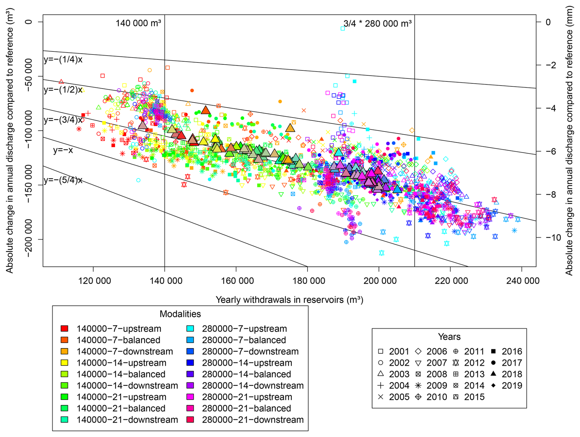
Figure 9 Yearly withdrawals in reservoirs compared with the annual absolute change in outlet discharge in m³ (left y axis) and in mm (right y axis) for all situations and all simulated years. Withdrawals and annual outlet discharges are computed from April of year n to March of year n+1. Larger colored triangles correspond to the mean values over the 20-year period for each situation.

In situations with 140 000 m³ of storage capacity, withdrawals are always higher than in situations with $\mathrm{3}/\mathrm{4}$ of the capacity threshold (and even higher than the total capacity). This level of withdrawal is possible only if the reservoirs are partially refilled during summer. In situations with 280 000 m³ of storage capacity, withdrawals are always lower than the total capacity but sometimes exceed the $\mathrm{3}/\mathrm{4}$ threshold.

The mean interannual values for each simulation (the large colored triangles in Fig. 9) align with the line $y=-(\mathrm{3}/\mathrm{4})x$ (except for 2 simulated situations). Thus, on average, $\mathrm{3}/\mathrm{4}$ of the irrigation water is used by the plants or evaporated. The remaining $\mathrm{1}/\mathrm{4}$ returned to the hydrological network as irrigation return flow, defined as the portion of irrigation water that flows back to the hydrological network (Ketchum et al., 2023). Irrigation first increases soil water content. Then, the irrigated water can contribute to different fluxes, i.e. (i) crop transpiration, (ii) soil evaporation, and (iii) percolation. Irrigation return flows occur when part of the irrigated water percolates to groundwater, which increases water table levels and streamflows. Since percolation only occurs when soils water content is above field capacity, irrigation return flows can be delayed compared to the irrigation period. The timing and amount of irrigation return flow can be critical for understanding the effects of small reservoirs, not only on outlet discharges, but also on low flows. These return flows can explain why, for some years, the autumnal outlet discharge increases compared to the reference situation (e.g. 2002, 2005, 2006, 2011, 2017). These return flows occur at reach sections that are located near irrigated fields, and can locally sustain flows during dry period. That explains why the proportion of network in low-flow decreases for some years, especially in autumn (e.g. 2001, 2016, 2017). To explain the variability observed in Fig. 9, we can make different assumptions:

1. Depending on the year and the situation, the reservoirs can be full or not at the beginning or at the end of the year. Some impacts can thus be deferred from one year to another.

2. Depending on the year (weather events) and the situation (location of irrigable crops and species), the efficiency of irrigation can differ.

3. Depending on the year and the situation, the balance of rainfall to evaporation on reservoirs can be different, which can affect the impacts more or less (see the Supplement for more information on the annual balance of rainfall, evaporation, and withdrawals).

3.4.2 Timing of withdrawals and reservoir refill

When a reservoir is not full, it collects all the upstream flows, and only the regulatory minimum flow is transmitted downstream, leading to discontinuities in the stream flow. These discontinuities can be critical for understanding the temporal dynamics of reservoir impacts. In our experiment, withdrawals from small reservoirs are highly seasonal. They occur in spring and summer, and most of them are related to the irrigation of maize and soybeans in summer. At the beginning of spring, the small reservoirs are usually full (the volume is close to 0 in Fig. 10). There are exceptions each year, when reservoirs are not full at the beginning of spring, which partially confirms the first hypothesis above. In most years, the reservoirs are also full at the beginning of summer. Hence, in spring, the discharges in the hydrological network and the rainfall over the reservoirs are usually high enough to compensate for withdrawals and evaporation. At the beginning of autumn, the reservoirs are usually not full, meaning that the withdrawals in summer are compensated not only during summer, but also in autumn and sometimes in winter. As a consequence, the stream is disconnected at the location of filling reservoirs during all this time. However, the variability between the years is high, and there are years in which reservoirs are already nearly full at the beginning of autumn (e.g., 2002, 2005, and 2006). Since stocks and withdrawals are more important in situations with higher storage capacities, the volume to refill after the irrigation campaign is usually much higher in these situations.

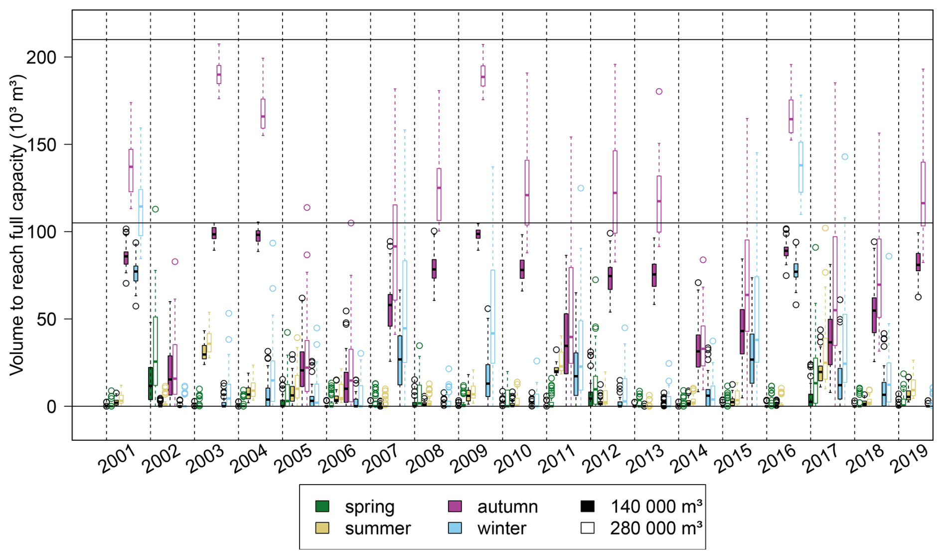
Figure 10 Boxplot of the volume needed to reach the maximum storage capacity in reservoirs at the beginning of each season for situations with 140 000 m³ (plain boxes) and 280 000 m³ (empty boxes) of total storage capacity. The black horizontal lines indicate $\mathrm{3}/\mathrm{4}$ of total storage capacity. n=45 per box.

4 Discussion

Our numerical experiment was designed to test the assumption that the spatial characteristics of a reservoir network influence its hydrological impacts. This work was driven by 4 main original ideas: (i) the impacts can vary from one year to another depending on the interannual variability of the climate; (ii) the impacts can vary throughout the year and must be analyzed seasonally; (iii) the impacts must be analyzed considering the stream flow along the entire stream network and not only at the outlet; and (iv) not only the influence of the spatial characteristics but also the processes behind the impacts of reservoirs must be analyzed.

The numerical experiment is based on randomly generated reservoir networks, composed of only small dams. The tested values for reservoir density and capacity cover a large variety of situations found southwestern France. It is difficult to estimate whether the distributions of reservoirs in the hydrological network are realistic. In particular, the randomness of the process can lead to situations with many reservoirs on a low-order stream. In the Gélon catchment, there are low-order portions of the network with up to three small reservoirs, so we considered that such configurations are also likely to occur.

The experiment was performed in only one catchment and its agro-pedo-climatic context, characterized by the presence of multiple shallow aquifers that drive most flows and the intensive use of small reservoirs for crop irrigation during the driest season (Table 3). This context is representative of southwestern France, and similar conditions are also encountered in other regions of the world, especially in Europe. In the following sections, we discuss aspects that are original and relevant for any context that involves small farm reservoirs.

4.1 How do the characteristics of the reservoir network affect flows?

4.1.1 Interpretation of factors roles in the variability of impacts

Our study demonstrates that the characteristics of the reservoir network influence the hydrological impacts of reservoirs in a catchment and that this influence varies from one indicator to another and depending on their temporal aggregation (see Table 3). The hierarchization of the influence of different spatial characteristics of the network constitutes an original insight. In this section, we try to understand how reservoirs modify flow and explain the influence of the factors studied.

Small dams modify flows in the hydrological network when they fill, reducing downstream flow. They fill because they lose water, either because of evaporation or because of agricultural withdrawals (and eventually because of leakage). In the numerical experiment, we show that flows in the hydrological network can be modified by a second process: the return flow of irrigation, which are flows that would not occur in the absence of withdrawals for irrigation. Depending on the characteristics of the reservoir network, withdrawals (and evaporation) and return flows occur in different locations of the hydrological network and possibly at different times, and their amounts differ. These differences can explain the influence of the characteristics of the reservoir network on the impact indicators.

On an annual time scale, the decrease in outlet discharge should be proportional to the total amount of water used to fill the reservoirs this year. Our study reveals that, in our context, the mean interannual withdrawals in reservoirs and the decrease in outlet discharge are proportional, indicating that withdrawals are particularly important for explaining the variability between simulations. Any characteristic of the reservoir network that increases withdrawals also increases the impact on annual outlet discharge. In our experiment, the total capacity is a strong limiting factor for withdrawals, which explains why it most affects the change in outlet discharge. This can certainly be generalized to any context in which reservoir capacity is a limiting factor for agricultural withdrawals.

In the summer, the storage capacity does not influence the outlet discharge, which means that the difference between simulations is not caused by a difference in the amount of withdrawals. The main factor is the distribution of reservoirs along the stream. In our context, reservoirs are intensively used during summer and, therefore, are partially empty. In this case, all upstream inflow in a reservoir, minus the minimum required flow, is stored, which means that the discharge at the outlet is composed mainly of water flowing in unequipped parts of the hydrological network. This explains the influence of the distribution of reservoirs. This result is likely to be expected in all situations with strong seasonality of withdrawals in small dams, which occur when stream flow naturally decreases. Therefore, studies that aim to assess the subannual variability of outlet discharge should consider the distribution of reservoirs in their models. For global approaches that aggregate multiple reservoirs located in an area (catchment or subcatchment), the total area drained by reservoirs can be a first indicator to describe the distribution of reservoirs, as is sometimes done (e.g. Meigh, 1995; Hughes and Mantel, 2010; Rabelo et al., 2021). An interesting follow-up to our study would be to test this assumption.

In our experiment, the spatial characteristics of the reservoir network, i.e. the number and distribution of reservoirs, are the main factors that influence the annual and summer proportions of network in low-flow for most years. The high influence of the number of reservoirs can easily be interpreted as follow: a greater number of reservoirs means a greater number of disconnection points in the hydrological network during the irrigation period when all reservoirs irrespective of their size are filling and therefore a greater length of network impacted by these disconnections. Surprisingly, the storage capacity has a limited influence on annual low flows. This means that the total amount of withdrawals (i.e. the volume required to fill the reservoirs) also has little effect on annual low flows. We can assume that after the first rainfall events in which groundwater is refiled, the baseflow is high enough to fill all reservoirs quickly.

The interpretation of the influence of the distribution of reservoirs on the summer proportion of network in low flow is more complicated. We can make different assumptions: (i) the distance of impacts of a single reservoir could be more important if it is located downstream because it affects a greater proportion of the downstream flow, and (ii) the downstream distribution leads to a concentration of reservoir on the main branch of the hydrological network, which could trigger complex interaction effects. These assumptions could not be verified in this study. In autumn, the factors influencing low-flow greatly vary from year to year. In dry years, the storage capacity has the main influence, which can only be interpreted by the presence of irrigation return flows after the end of the irrigation period, which locally increase flows. At the end of the irrigation period, the soil water content is higher for irrigated crops (and higher in situations with more irrigation), and lower rainfall rates are required to refill aquifers and increase baseflows.

4.1.2 How do these results generalize?

The impacts of small reservoirs on spatialized low flows and outlet discharge and the effect of the different factors result from: (i) a natural seasonality in flow regimes, (ii) a strong seasonality of withdrawals, which occur when streamflows decrease, and (iii) limited restrictions on reservoir management, and especially no restriction on filling dates. These three components are common in many situations with small reservoirs around the world, even with different climates and types of hydrological functioning. This means that most of our analysis still stands in such situations, eventually with local specificities.

In our study, there are three specificities: the minimum required flow, the dead volume practice, and the presence of irrigation return flows. The minimum required flow is generally lower than the low-flow threshold used for the low-flow indicators, which means that the portions of the network located downstream of a filling reservoir will always be in low flow, as if there was no minimum required flow (more information is provided in the Supplement). The dead volume practice implies that there are no withdrawals when reservoirs reach $\mathrm{1}/\mathrm{4}$ of their capacity, but that evaporation can continue. For the same utilizable capacity (e.g. 210 000 m³ for situations at 280 000 m³ of storage capacity with $\mathrm{1}/\mathrm{4}$ of dead volume), the total evaporation will be higher if there is a dead volume. In our context, this additional loss is probably small compared to total withdrawals, but in other contexts with a higher evaporative demand (e.g. in South Africa Meigh, 1995), this practice could substantially increase the impacts of reservoirs. The importance of irrigation return flows in our context is probably the result of intensive irrigation practices and a favorable morphological context. We are the first to report the presence of such return flows in a study on small farm reservoirs, but are also the first to use a modeling approach capable of showing their presence and to look for their existence.

In some regions of the world, such as Australia, Botswana, or South Africa, small reservoirs can also be used for stock watering (Meigh, 1995; Hughes and Mantel, 2010; Robertson et al., 2023). In catchments where watering is the main use of reservoirs, the withdrawals will be constant throughout the year and the influence of the network characteristics will likely differ. Considering the domain of validity of our modeling approach, our study tests the effects of small dams only. In our context, where groundwater drives most of the flows, hill reservoirs are usually directly connected to shallow groundwater or to drainage water and are most likely to have similar impacts as reservoirs located along the stream. However, we cannot generalize our results to all situations with hill reservoirs, especially for catchments with a greater contribution of surface runoff to stream flow.

4.1.3 A portion of non-explained variability

For all the indicators and for all the years, the residuals of the ANOVAs are quite important, usually accounting for more than 20 % (Fig. 8), which means that the characteristics of a reservoir network alone cannot explain all impacts. These residuals can be qualitatively attributed to complex interactions between reservoirs that are not captured by the three studied factors, to random effects due to the exact location of irrigable crops and the types of crops irrigated by each reservoir, and to legacy effects due to the meteorological and hydrological variability (e.g., impacts deferred from one year to the next for partially full reservoirs). The second point is important, as we considered that the impacts of reservoirs are caused by the infrastructure and the modification of nearby crops due to the opportunity created by the infrastructure. These elements contribute to the variability in the impacts of reservoirs, which is difficult to analyze. For example, the amount and timing of withdrawals will differ if a reservoir irrigates straw cereals only or maize only. For local water managers, these random effects are impossible to anticipate. Therefore, it is interesting to have included a random allocation of irrigable crops to reservoirs in the numerical experiment to consider the associated uncertainty.

4.2 Methodological advances

4.2.1 Assessment of low flow along the stream

Low flows are key characteristics of stream flow and are important for stream ecology (Sarremejane et al., 2022). They are the main concern of water managers in such agricultural catchments. Despite their scientific and management interests, low flows have rarely been quantified and analyzed in the context of small farm dams. In the literature, they have been characterized with flow duration curves (Q₉₅ or Q₉₀ as indicators of low flow) (e.g. Hughes and Mantel, 2010; Habets et al., 2014; Pinhati et al., 2020), with the number of days with outlet discharge lower than the historical median discharge (Robertson et al., 2023) or with the minimum mean discharge calculated for a sliding period of 30 d (Galéa et al., 2005). All these indicators are based on outlet discharges, which do not necessarily represent the hydrological state along the entire stream network. Maps of the variables listed above could help locate low-flow hotspots along the stream. Maps are used in some studies on small reservoirs to display the mean discharge over a period (e.g. Güntner et al., 2004; McMurray, 2006; Deitch et al., 2013; Lebon et al., 2022) but never to display information on low flows.

Our new indicator, the proportion of network in low flow, summarizes the hydrological state of the stream network in a single value. Our results show that the low flow at the outlet in the context of numerous small reservoirs on the hydrological network is not representative of the low flow experienced in the entire network, and that the proportion of network in low flow performs much better (Fig. 4). Furthermore, we show that the proportion of network in low flow is sensitive to the spatial characteristics of the reservoir network, i.e. the number and distribution of reservoirs. The indicator only provides information on the severity of low flow experienced on average along the stream. An interesting follow-up would be to develop an indicator that characterizes whether low flow occurs more or less downstream. A possible approach would be to build on the concept of downstreamness (Colombo et al., 2024). Mapping the number of low-flow days can also be a good way to study low flows spatially (Fig. 4). The presented maps reveal that the number of low-flow days at a given location depends on the distance to the upstream reservoirs and the location of these reservoirs. However, maps provide only snapshots of the impact for one simulation and one period. They could not be used in this study to compare the 90 simulations.

4.2.2 Addressing the interannual variability of climate, hydrology, and irrigation practices

Evaluating the impact of small reservoirs in a context of high interannual variability of climate and hydrology, such as in our study site (Fig. 3), remains challenging. Climate is an important forcing variable for hydrology, but also for crop growth and farming practices. Depending on the weather, a reservoir can be full or not at the beginning of the cropping season, and farmers will then irrigate their crops more or less depending on the crop water demand and water availability in the reservoir. One of the features of MHYDAS-Small-Reservoirs is the ability to simulate this dynamic interaction between crop demand and water availability resulting from the interannual variability of climate and hydrology.

In our experiment, the impacts of small reservoirs on outlet discharge and low flow are highly variable from year to year (see Fig. 6). This implies that an interannual mean of impacts is not necessarily representative of the hydrological stress caused by small reservoirs, and raises the question of how to perform the analysis of results to consider this interannual variability. In the literature, some authors chose to present their results for specific years only, usually a median year, a dry year, and a wet year in terms of rainfall (e.g. Tarboton and Schulze, 1991; Teoh, 2003; McMurray, 2006; Deitch et al., 2013; Habets et al., 2014; Lebon et al., 2022). This choice can be good if the climate can be easily classified into typical wet or typical dry years, which is not the case in our study (see Fig. 3). A year can be dry because of a dryer spring or a dryer summer, which will probably not result in the same impact. Furthermore, the weather conditions of a given year can impact the hydrology in the following year, for example in case of poor groundwater recharge, which makes the selection of a reduced set of years for analysis impossible. Finally, our results show that the contribution of each factor to the impacts also depends on the year (see Fig. 8), suggesting the existence of interactions between various processes that jointly depend on the characteristics of the reservoir network, the weather and the initial yearly conditions.

4.2.3 A strong seasonality of impacts

Indicators computed annually are useful, but they can hide a large temporal variability of impacts within the year. In our case, the annual impacts of reservoirs on outlet discharge can be considered low (−1 % to −6 %), but in the summer, the decrease is usually higher than 20 % and can reach the 60 %–70 % range, which is critical for the Gélon stream and for downstream rivers. For the proportion of network in low flow, the annual indicator shows an increase in low flow for most years, which actually results from an increase of the proportion of low flow during summer and a decrease during autumn. The subannual variability of the impacts on the outlet discharge has already been reported in the literature for monthly flows, either using statistics on multiple years (e.g., mean, median, flow duration curves, etc.) (e.g. in Ramireddygari et al., 2000; Savadamuthu, 2002; Alcorn, 2007; Cetin et al., 2009; Habets et al., 2014; Gautam and Corzo, 2023; Yan et al., 2023), or values for specific years (e.g. Tarboton and Schulze, 1991; Thompson, 2012; Dong et al., 2019). Other authors also choose a seasonal aggregation (e.g. Galéa et al., 2005; Perrin et al., 2012; Xu et al., 2013). In the literature, the subannual variability is usually explained by a combination of two processes: the natural variability in stream discharge and the seasonality of withdrawals. Our study reveals that, depending on the context, irrigation return flows can also contribute to this variability.

5 Conclusions

Our work constitutes a methodological advance and provides new insights into the hydrological impacts of small farm reservoirs and their driving factors. A spatially distributed agro-hydrological model was used to evaluate the impacts of 90 alternative reservoir networks in the same catchment. The model considers crop growth and management at the parcel level and includes a reservoir management model. The networks tested differed in terms of reservoir density, capacity, and spatial distribution, allowing us to study the effects of these factors on flow regimes throughout the year. The focus was on outlet discharges and low flows, for which a new indicator was developed to summarize the hydrological status of the entire hydrological network and not only of its outlet.

Although the experiment was conducted for only one catchment, our conclusions should remain relevant in many contexts characterized by a high seasonality of stream flow and withdrawals and the presence of numerous small dams with fill-and-spill functioning. Key lessons from the experiment are (i) an important annual variability of impacts and factor influence that needs to be properly analyzed; (ii) the need to consider not only annual but also seasonal indicators given the high subannual variability of the impacts found; (iii) the potential of maps to study the impacts of reservoir on low flows and the capacity of our new indicator to characterize the severity of low flows experienced along the stream; (iv) the main explanatory factors to explain the variability in discharges and low flows being alternatively the storage capacity, the number of reservoirs or their spatial distribution; and (v) the key processes linked with these factors being the disconnections in the hydrological network caused by reservoir refill and the return flows of irrigation, both driven by the amount, timing, and location of withdrawals.

In this study, we focus on the influence of the physical characteristics of the reservoir network. A next step will be to test the impact of different management rules or to explore scenarios with different cropping systems. More generally, the approach used in our work for the numerical experiment could easily be applied even in different hydrological and agricultural contexts, provided that models are available for these other managements and contexts.

This work could help support the choice of a representation of small reservoirs in hydrological models depending on the impact indicator relevant for the study, as different properties of the network appear critical to assess different indicators across different timescales. Finally, our work can also help water managers to better identify the drivers behind the hydrological impacts of small reservoirs and guide them in their decision making.