Multi-site learning for hydrological uncertainty prediction: the case of quantile random forests

To improve hydrological uncertainty estimation, recent studies have explored machine learning (ML)-based post-processing approaches that enable both enhanced predictive performance and hydrologically informed probabilistic streamflow predictions. Among these, random forests (RF) and their probabilistic extension, quantile random forests (QRF), are increasingly used for their balance between interpretability and performance. However, the application of QRF in regional post-processing settings remains unexplored. In this study, we develop a hydrologically informed QRF post-processor trained in a multi-site setting and compare its performance against a locally (at-site) trained QRF using probabilistic evaluation metrics. The QRF framework leverages simulations and state variables from the GR6J process-based hydrological model, along with readily available catchment descriptors, to predict daily streamflow uncertainty. Our results show that the regional QRF approach is beneficial for hydrological uncertainty estimation, particularly in catchments where local information is insufficient. The findings highlight that multi-site learning enables effective information transfer across hydrologically similar catchments and is especially advantageous for high-flow events. However, the selection of appropriate catchment descriptors is critical to achieving these benefits.

1 Introduction

1.1 On the need for quality uncertainty estimates

Providing quality uncertainty estimates for streamflow predictions is critically important, particularly in applications such as operational drought simulation, water resource management, and flood mitigation where significant stakes are involved (Hwang et al., 2019; White et al., 2017). Poorly quantified or overly confident predictions can lead to misinformed decisions, potentially resulting in economic losses, infrastructure damage, or even threats to public safety. To address this, various approaches have been proposed in the hydrological community for streamflow uncertainty quantification, including multi-model ensembles (Georgakakos et al., 2004; Troin et al., 2021), Bayesian inference (Kuczera and Parent, 1998; Bates and Campbell, 2001), and hydrological error modeling (Krzysztofowicz, 1999; Todini, 2008; Solomatine and Shrestha, 2009; Bennett et al., 2021), referred to as post-processing. Post-processing involves a process-based model followed by a statistical approach to correct errors and quantify the associated uncertainties. With the post-processing procedure, uncertainties can be quantified by modeling the error patterns based on an archive of past data.

Hydrological post-processing techniques were adopted early through methods such as the hydrological uncertainty processor (HUP) (Krzysztofowicz, 1999) and model conditional processor (MCP) (Todini, 2008), but recent machine learning (ML)-based approaches have emerged as powerful tools for hydrological post-processing. Although less interpretable, ML-based approaches can potentially produce reliable and more informative uncertainty estimates (Papacharalampous and Langousis, 2022; Tyralis and Papacharalampous, 2024). Methods such as quantile regression (QR) (Tyralis et al., 2019; Papacharalampous and Langousis, 2022), conformal prediction (Auer et al., 2024), and random forests (Zhang et al., 2023) have been used for streamflow post-processing with promising results. However, ML algorithms can produce different uncertainty estimates depending on how they are trained – particularly on which catchments are included in the training dataset. Since hydrological conditions vary significantly across catchments, the selection of catchments used for training can influence the uncertainty estimates of the ML model. In our study, we aim to explore whether including different catchments, referred to as regional or multi-site learning, may improve ML-based post-processing for error-correction and uncertainty prediction, and specifically for the quantile random forests (QRF) model. A QRF model for error-correction and uncertainty prediction trained in a regional setting can leverage information across several catchments. In contrast, local at-site approaches train models independently for each catchment and cannot benefit from error patterns shared in hydrologically similar catchments.

1.2 Machine learning-based post-processors

Random forest (RF) (Breiman, 2001) and its probabilistic variant, quantile random forest (QRF) (Meinshausen and Ridgeway, 2006) are extensively used and are considered state-of-the-art in many hydrological applications. Recently, Zhang et al. (2023) compared the QRF model and the countable mixtures of asymmetric Laplacians long short-term memory (CMAL-LSTM) model to probabilistically post-process streamflow simulations across 522 catchments. The QRF and CMAL-LSTM models were comparable in terms of uncertainty estimates, but the CMAL-LSTM deep learning (DL) model performed better in catchments with large flow accumulation areas. QRF has also been applied in hydrologically informed post-processing approaches. Shen et al. (2022) used in an RF framework and leveraged internal state variables to correct PCR-GLOBWB (PCRaster Global Water Balance, a global hydrological model) simulations at three stations in the Rhine Basin. They found that the use of hydrological model states as input features of RFs provides additional information that may not be included in the model simulations. However, challenges remain, particularly in modeling errors during high streamflow periods. Magni et al. (2023) expanded the same approach at a global scale, using PCR-GLOBWB model simulations and internal states, in conjunction with static catchment attributes, to train a single RF model on a global database of streamflow simulations and measurements. They found that improvements were independent of the availability of streamflow data, indicating the power of regional learning methods in poorly gauged and ungauged catchments.

Prediction in ungauged basins is not the only benefit of training a single ML model on data from multiple catchments. Kratzert et al. (2024) advocated the use of regional approaches to fit a deterministic Long Short-term Memory (LSTM) DL model for streamflow simulations. They found that larger LSTM models trained on all available basins outperform smaller models trained on a limited set of catchments. This is because some ML approaches can properly use the additional information contained in larger training sets to perform better than models specialized for individual catchments(Montero-Manso and Hyndman, 2021). Furthermore, Johnson et al. (2023) found that hydrological model performance depends on catchment characteristics, indicating the presence of regional bias, where hydrological errors exhibit similar properties for neighbouring catchments. This can be harnessed to improve uncertainty estimation using a post-processing model with a regional parametrisation and trained on hydrological errors from multiple sites. We intend to consider these catchment characteristics as additional input features within the proposed post-processing model.

1.3 Scope of this study

This study addresses uncertainty estimation of process-based hydrological model simulations, with a focus on streamflow reconstruction and future projection scenarios. We investigate the added value of multi-site post-processing applied to a quantile random forests (QRF) model. The main contributions of this work are: (i) to understand the impact of including different catchments in the training process of QRF (multi-site) on the quality if its uncertainty estimates and (ii) to investigate the importance of catchment characteristics for these multi-site QRFs. Although multi-site approaches can benefit the modelling of ungauged catchments, our work specifically addresses improvements in uncertainty estimation for catchments with available streamflow measurements.

Accordingly, we use temporally varying information (predicted streamflows and model states) in addition to catchment dependent characteristics to estimate uncertainties in hydrological model predictions. We chose to focus on QRF due to its balance of performance, interpretability, and popularity in the hydrological community. To the best of our knowledge, no prior study has explored the impact of multi-site learning with the QRF algorithm for uncertainty estimation, particularly when post-processing a hydrological model calibrated separately for each catchment. To that end, we fit different QRF variants on the internal states of a hydrological model, on meteorological variables, and on readily available catchment characteristics. The proposed regional QRF variants are evaluated across a large sample of 564 French catchments to identify when multi-site learning may be beneficial and to offer practical considerations for multi-site QRF applications.

The paper is organized as follows: We first introduce the dataset and describe the QRF algorithm, its variants, and the probabilistic evaluation framework. Then, we present and discuss the results before summarizing the key findings along with implications for future work.

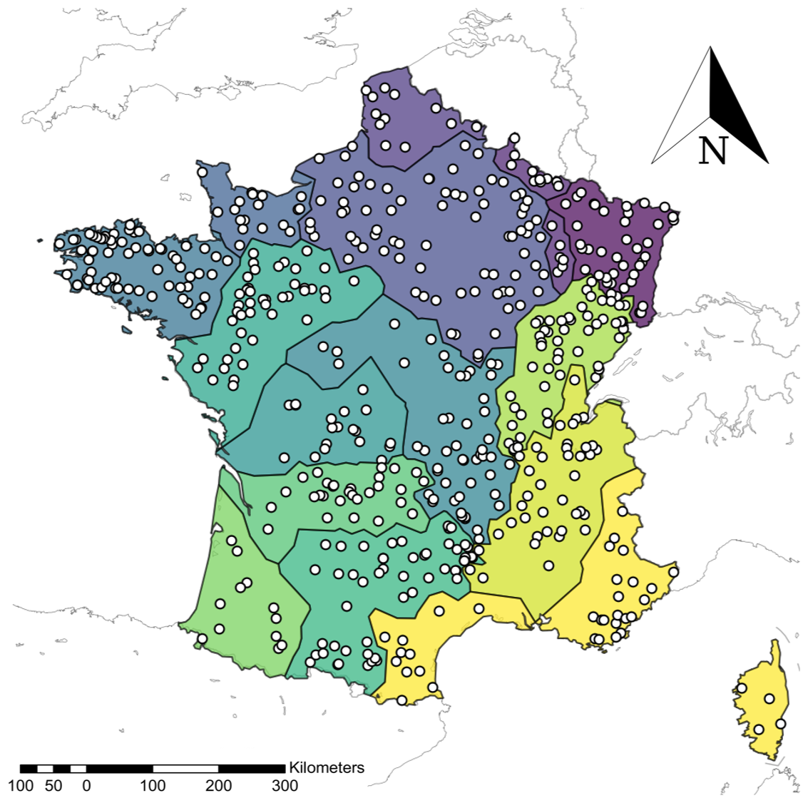
Figure 1 Location of the 564 catchment outlets. Plotted regions represent the hydroclimatological catchment groups used in the study.

Table 1 Features used in the study.

2 Dataset

2.1 A dataset of 564 French catchments

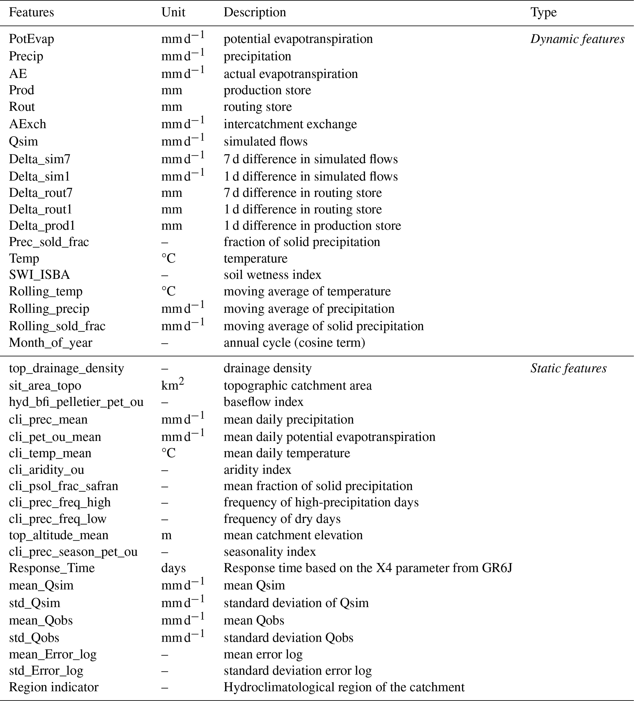
We used a set of 564 catchments distributed throughout France (Fig. 1). These catchments represent a wide range of hydrological regimes and simulation contexts. We selected these catchments from the CAMELS-FR hydroclimatic dataset (Delaigue et al., 2025). The criteria for selecting these catchments were as follows: (i) low anthropogenic influence, (ii) good data quality for all flow regimes, and (iii) an available time series longer than 21 years. Streamflow data were obtained from the national HydroPortail archive (Leleu et al., 2014; Dufeu et al., 2022) at a daily time step for the period 1977–2021. Meteorological forcings (precipitation and temperature) were provided by Météo-France's daily SAFRAN grid reanalysis (Vidal et al., 2010). Potential evaporation (PET) is calculated using the formula proposed by Oudin et al. (2005) and requires two inputs: extraterrestrial radiation ($\mathrm{MJ}{\mathrm{m}}^{-\mathrm{2}}{\mathrm{d}}^{-\mathrm{1}}$) and mean daily air temperature (°C). Extraterrestrial radiation is computed as a function of the localization of the basin and Julian day values and the temperature is the only dynamical meteorological input used to estimate PET. Since our interest is in developing a multi-site QRF post-processor, we used several static basin-averaged attributes describing climate, topography, and geology. All of these attributes are included in the CAMELS-FR dataset and are listed in Table 1.

Hydrological calibration was performed independently for each catchment over the 1977–2021 period. Subsequently, the QRF variants were implemented using a standard train–validation–test split over the 1990–2021 period:

• P1: training period from 1990 to 2004, used to train the QRF post-processor.

• P2: validation period from 2005 to 2009, used to select the hyperparameters of the QRF post-processor.

• P3: testing period from 2010 to 2021, used to test the performance of the QRF variants on new data.

2.2 Methods

2.3 Hydrological model

We used discharge simulations obtained with the GR6J rainfall–runoff model (Pushpalatha et al., 2011), a daily 6-parameter conceptual lumped model. GR6J has been applied in several studies across a large number of catchments and hydroclimatic contexts (e.g. Poncelet et al., 2017; Golian et al., 2021; Tanguy et al., 2023). The GR6J model is based on several state variables that control its simulations, in particular, the production and routing store levels, as well as intercatchment exchange fluxes. We intend to use these state variables as predictors in the QRF algorithm. Shen et al. (2022) successfully used internal state variables as predictors in an RF framework to correct hydrological model errors. They found that internal state variables provided valuable information for the RF, enabling it to detect and correct for systematic hydrological model errors. To account for the influence of snow in some catchments, we incorporated Cemaneige (Valéry et al., 2014), a snow accumulation and melt model, with constant parameters for all catchments.

The Cemaneige-GR6J model was calibrated using the airGR R package (Coron et al., 2017, 2023) using the built-in calibration algorithm. To ensure good performance across a wide range of streamflow conditions, the target optimization criterion was a combination of KGE based criteria (Gupta et al., 2009; Kling et al., 2012): an equal weighting of KGE criteria with power transformations of 0.5 and −0.5 applied to streamflow, as detailed in Appendix C. This calibration approach was implemented to obtain the six parameters of GR6J: production store capacity (mm), groundwater exchange coefficient (mm d⁻¹), routing store capacity (mm), time constant of unit hydrograph (days), groundwater exchange threshold (–), and exponential store coefficient (mm).

2.4 Feature selection and data transformations

2.4.1 Target variable

For this study, we model the probabilistic distribution of hydrological model errors. Since these errors are skewed and non-Gaussian (e.g. Evin et al., 2014), we applied a logarithmic transformation to improve the training process:

$$\begin{array}{}\text{(1)}& {\mathit{ϵ}}_{\mathrm{t}}=\text{log}\left({\displaystyle \frac{Q_{\mathrm{t}}^{\text{obs}}+\mathit{\delta }}{Q_{\mathrm{t}}^{\text{sim}}+\mathit{\delta }}}\right)\end{array}$$

where ϵ_t is the target variable of our study and represents the prediction error, $Q_{\mathrm{t}}^{\text{obs}}$ and $Q_{\mathrm{t}}^{\text{sim}}$ indicate observed and simulated streamflows, respectively (mm d⁻¹), and t represents the time index with a temporal step of 1 d. δ is an offset parameter to avoid zero streamflow values and is unique for each catchment. It was calculated following the recommendation in Pushpalatha et al. (2012). The use of δ is especially relevant in this study due to the application of the logarithmic transformation.

The input predictors (or features) in the QRF models are listed in Table 1. These features can be broadly categorized into two groups of approximately equal size: (i) time series data (dynamic features) that capture temporal variability, and (ii) catchment descriptors (static features) that enable spatial identification of catchments.

2.4.2 Dynamic features

The proposed QRF framework post-processes GR6J simulations and uses hydrological model outputs and state variables along with meteorological inputs (precipitation and temperature). Streamflow uncertainties are known to be autocorrelated (Evin et al., 2014), with strong autoregressive (AR) and memory effects. Consequently, lagged observed streamflow (Zhang et al., 2023; Pham et al., 2020) is a popular input feature for RF-based post-processing. In the simulation context of this study, streamflow observations are not available for streamflow reconstruction and projection scenarios, and we use state features from the GR6J model to provide additional information to QRF. Although some of the features in Table 1, such as simulated flows and production store, are strongly autocorrelated, we assume that the additional information still leads to improved uncertainty estimates compared to using model simulations alone. Similarly to Shen et al. (2022), we include other temporal information in QRF through transformed features: (i) increment features of hydrological model simulated streamflow and states to help capture the dynamics of the hydrograph (rising and falling limbs etc.) and (ii) moving averages of meteorological features to highlight general trends. This feature engineering step can be relevant for RF-based algorithms in a time series context, because QRF does not create temporal memory or embeddings as is the case for AR models and LSTM neural networks (Evin et al., 2014; Li et al., 2016; Kratzert et al., 2018). In this context, the selected moving average filter size is equal to the catchment response time, which was obtained from the time constant of the unit hydrograph parameter of the GR6J model.

2.4.3 Static features

To take into account spatial heterogeneity, catchment descriptors are used for the multi-site QRF variants. The static features include (i) average catchment attributes such as catchment area and aridity index. We chose to keep thirteen relevant catchment attributes following the recommendations of Jehn et al. (2020); (ii) scale features of errors, simulated flows, and observed streamflows. These scale features provide additional unique indicators of catchment characteristics. Montero-Manso and Hyndman (2021) found that combining individual time series features such as catchment attributes with scale features can improve the performance of ML models in a deterministic setting. Similar improvements are expected for QRF in the setting of hydrological uncertainty estimation. It is important to note that these scale features are not available for prediction in the context of ungauged catchments, as they are calculated based on observed streamflows.

Figure 2 Schematic overview of implementing QRF based post-processors. Configurations 1, 2, and 3 represent the regional information used in QRF post-processing. A description of the features used is provided in Table 2.

2.5 QRF: how to fit the algorithm?

Random forest Breiman (2001) is a non-parametric ensemble tree-based model that offers good performance and provides certain interpretability through its feature importance estimates (Breiman, 2001; Breiman et al., 2017). RF and its probabilistic version QRF are used extensively in the hydrometeorological domain. An important advantage of QRF is that it provides full distributional estimates without the need to estimate each quantile separately, as is required in quantile regression (Tyralis et al., 2019; Papacharalampous and Langousis, 2022). QRF has been applied to complex and heteroscedastic cases, including hydrometeorological ensemble forecasts (Taillardat et al., 2016; Tiberi-Wadier et al., 2021; Teja et al., 2023), post-processing of streamflow simulation (Zhang et al., 2023), and estimation of the limits of acceptability for hydrological models (Gupta et al., 2024). Further details on the construction of RF and QRF can be found in Louppe (2014); Meinshausen and Ridgeway (2006), but, QRF can be viewed as an analog method (Delle Monache et al., 2013; Hu et al., 2023) that performs a weighted nearest-neighbor search for analogous events. Similarly to a classic RF, QRF grows a number of trees n, with each tree trained on a bootstrapped subsample of the original training data.

Individual trees are trained according to the Breiman et al. (2017) algorithm by minimizing a loss function and making successive splits with a predefined number of features p. This tree-building process enables QRF to account for strongly correlated features, which is important given the strong correlation of some of the features used. For the purpose of this study, we use mean squared error (MSE) as a loss function to calculate the homogeneity of each group. The procedure continues recursively, with each resulting group split further until a minimum number of data points m in child splits is reached.

In the classic Random Forest (RF) algorithm, predictions from individual trees are averaged to produce a single deterministic output. In contrast, Quantile Regression Forest (QRF) leverages the leaf nodes of trees to compute proximity measures between a test input and training instances. For a prediction at time t and given input x_t, each QRF tree is traversed using binary splits to reach a corresponding leaf node. A proximity weight ω_i(x_t) is then defined for each training instance i (Meinshausen and Ridgeway, 2006), which is then used to estimate the cumulative distribution function (CDF) of the prediction uncertainty:

$$\begin{array}{}\text{(2)}& \widehat{F}\left(\mathit{ϵ}\right|x_{\mathrm{t}})=\sum _{i=\mathrm{1}}^n{\mathit{\omega }}_i(x_{\mathrm{t}}){\mathrm{1}}_{\mathit{\{}{\mathit{ϵ}}_i\le \mathit{ϵ}\mathit{\}}}\end{array}$$

where ω_i(x_t)>0 and ${\sum }_{i=\mathrm{1}}^n{\mathit{\omega }}_i\left(x_{\mathrm{t}}\right)=\mathrm{1}$, ϵ_i denotes the hydrological error of training instance i, and $\widehat{F}$ is the estimated CDF of uncertainty for x_t.

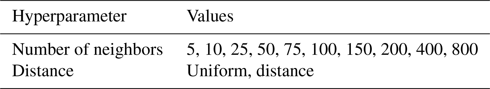
To provide reliable and sharp uncertainty estimates, we considered three hyperparameters for optimization: (i) The minimum number of samples at child nodes m, which affects tree depth and strongly impacts reliability and sharpness. Setting high values for the minimum samples per leaf might yield high reliability, but can lead to poor performance, as the trees are too general and information is lost. Low values result in overfitting and unreliable uncertainty estimates. (ii) The number of features per split, p, which also shapes the QRF uncertainty estimates. Higher values can lead to under-dispersed uncertainties, while lower values may reduce sharpness. (iii) The number of trees n, which controls precision and stability. A larger number of trees improves the quality of uncertainty estimates, but improvements diminish as computational cost increases, especially in larger models. Further details on hyperparameter values and selection are provided in Sect. 2.7. Additionally, we also use a K-nearest neighbor (K-NN) (Wani et al., 2017) approach as a benchmark for the QRF methods used in the study. Like QRF, K-NN aims to find analogous events but based on the Euclidean distance between features. Here, K-NN is fitted locally on the same variables as for QRF. Further details on the fitting process and the hyperparameters used are provided in Appendix B.

Given Eq. (2), the estimated CDF is bounded by the training sample. QRF is unable to predict a quantile higher than the maximum observed in the training sample, which implies that QRF trained on a single basin is constrained by the range of errors in its training data. A more hydrologically diverse training dataset would alleviate this problem and enable QRF to adapt to more extreme events, provided that QRF is able to use the additional information properly.

Table 2 QRF variants of the study.

2.6 QRF variants

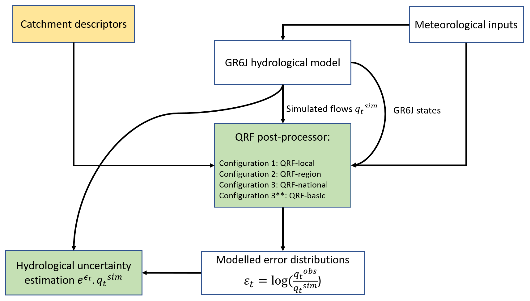
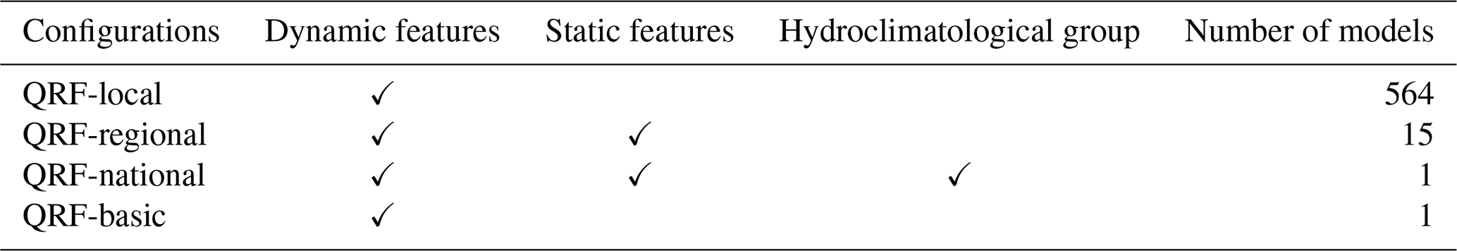
Figure 2 presents the framework employed for the QRF configurations analyzed in this study. The local approach (QRF-local) refers to training the QRF algorithm on data from a single basin. Given their construction, spatial features are constant for each individual catchment and only time-series features can be fed to QRF in the local setup. QRF-local yields 564 independently trained QRF models, each specific to its respective catchment. Next, spatial variability is added as we extend QRF to a multi-site setting. The objective here is twofold: (i) to examine whether spatial diversity can improve the uncertainty estimates of QRF. This can be challenging, particularly since the used GR6J hydrological model is calibrated on an on-site basis; and (ii) to determine the optimal number of catchments to include in the training set for effectively capturing hydrological diversity and improving QRF predictions. We test QRF with two spatial settings: (i) a regional approach (QRF-region), where QRF is trained on data from catchments that are geographically close and thus potentially have similar error dynamics. In total, 15 regional QRF models are developed for the hydrological regions of the study (see Fig. 1), based on hydroclimatological groupings of French catchments; (ii) a global approach (QRF-national), in which a QRF is trained on data from all catchments in the dataset. Both static and dynamic descriptors are used in the training process of QRF-region and QRF-national. However, QRF-national uses the catchment's hydrological region as an additional input feature, which cannot be used for QRF-region. Intuitively, in cases where QRF is unable to transfer information from different basins or when there are no useful analogs in similar catchments, QRF-local would yield better performance, as no information from other catchments is used to build the model. To assess the usefulness of static features for the multi-site QRF setup, we included QRF-basic, a global QRF approach fitted on all catchments of the study, but only with dynamic features. This experiment is expected to highlight whether dynamic time series features are sufficient to improve multi-site QRF predictions or that static features are essential for multi-site post-processing. Table 2 presents the features used in the three configurations. The QRF models used in this study was fitted using the quantile-forest Python library (Johnson, 2024).

It is worth mentioning that in multi-site setups, the standardization procedure is an essential step that enables QRF to determine analogs across a set of diversified catchments, as the scales of streamflows and dynamic features (GR6J states and transformed variables) vary significantly. Standardization is important for a meaningful training process and for the identification of adequate analogous events. Initially, we standardized input data via the popular standard scaling method (Hastie et al., 2001), which transforms dynamic features – for each catchment – so that the average and standard deviation are set to 0 and 1, respectively. However, the method resulted in inconsistencies for catchments with outliers, as the standard deviation is sensitive to extreme values. To solve this issue, we opted for robust standardization (Hastie et al., 2001), which removes median values of dynamic features and the target errors ϵ_t defined in Sect. 2.3.

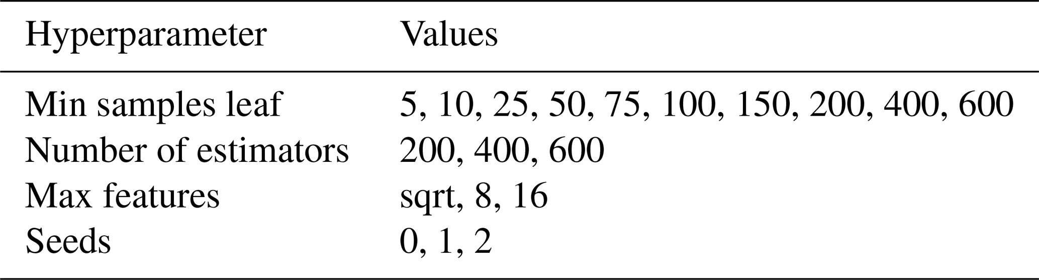
2.7 QRF hyperparameters

Since we use QRF for probabilistic predictions, hyperparameter selection was based on the mean of the alpha score and CRPSS values. This would enable a selection based on the quality of overall uncertainty estimates with an emphasis on reliability. For QRF-local, hyperparameters were tuned independently for each catchment and the set maximizing the aforementioned criteria during the validation period was selected. QRF-region and QRF-national hyperparameters were selected based on median criteria among the regions' catchments. The selection criteria for QRF-local are specific to each catchment, which is expected to enhance the results of the local model compared to approaches that use fixed hyperparameters across multiple catchments. Table 3 presents the hyperparameters selected for optimization.

Table 3 Hyperparameters set optimized for QRF.

3 Assessment criteria

In this section, we present the probabilistic metrics used to evaluate the three variants of QRF. The criterion followed for probabilistic predictions conforms to Gneiting et al. (2007)'s objective of maximizing reliability subject to sharpness. In this context, reliability refers to the statistical consistency between the predicted uncertainty distributions and the observed streamflow values, while sharpness is a property of predictions exclusively and refers to the magnitude of the uncertainty distributions. In practice, uncertainty estimates that closely align with observed streamflows are more accurate and reliable, while predictions with smaller magnitudes are considered sharper. To assess these properties, we used two types of metrics. Distributional metrics evaluate the full predictive distribution, while interval metrics focus on a pre-specified predictive interval. As presented below, reliability is measured by the alpha score and the coverage ratio. For assessing sharpness, we used the dispersion score and average width interval. Additionally, deterministic evaluation criteria were also used to provide a more holistic assessment of the proposed QRF variants. Each variant predicts 200 quantile members at each time step 200 quantile members equally spaced between 0.005 and 0.995. The scores are calculated using the EvalHyd (Hallouin et al., 2024) Python library.

3.1 Distributional metrics: alpha score, dispersion score, and CRPSS

The alpha score (Renard et al., 2010) targets reliability. It calculates the closeness of predicted uncertainty distributions to the statistical distribution of observed streamflows. If the uncertainty distributions of streamflows are reliably quantified, the observations correspond to realisations from the uncertainty distributions of streamflows. In practice, the alpha score compares the empirical distribution of the probability integral transform (PIT) values to the uniform distribution on [0,1]. A perfect alpha score corresponds to uniform PIT distributions while deviations of PIT values from the uniform distribution indicate lower reliability. The values of the metric range from 0 (worst reliability) to 1 (perfect reliability).

For sharpness, we used the dispersion score calculated as a skill score following Bontron (2004). The method consists in computing the continuous ranked probability score (CRPS; Gneiting et al., 2005) by comparing uncertainty distributions with their medians, as detailed in Appendix E. This formulation targets the magnitude of the distributions instead of the agreement with the observations. To obtain a positively oriented score, the dispersion score is expressed as a skill score by dividing by the same quantity computed for the climatological distribution. The resulting metric scores 1 for a perfect point prediction; positive values indicate better sharpness compared to the climatological distribution, while negative values indicate worse performance.

We also compute CRPS by comparing uncertainty distributions to observed streamflow values, which allows to assess both reliability and sharpness. We express CRPS as a skill score (CRPSS) relative to the climatological distribution, and similarly to the dispersion score, CRPSS equals 1 for perfect point prediction; positive values indicate better performance than the climatological distribution, while negative values indicate worse performance. Throughout the study, the empirical distribution of observed streamflows is defined over the training period, as detailed in Appendix E.

3.2 Coverage ratio, average interval width, and Winkler score

To provide a more comprehensive assessment of predictive uncertainty, evaluation metrics were calculated for prediction intervals at the 90 % and 95 % confidence levels. The coverage ratio (CR) is a measure of reliability that counts the proportion of observations that lie within the prediction intervals. Values closest to the desired coverage level (i.e., 90 % or 95 %) are best. Scoring lower values diminishes the utility of the model (under-coverage), while scoring higher values than the desired coverage is less problematic, but indicates that the model can provide sharper intervals (over-coverage). Moreover, it is worth highlighting that the two metrics used to assess reliability are closely related: the coverage ratio reflects reliability at a specific confidence level, while the alpha score aggregates coverage across all confidence levels. To assess the sharpness, we employ the average width metric (AW), which corresponds to the average width of the prediction interval during the evaluation period. We also evaluate the Winkler score (WS), which simultaneously includes both criteria, and enables an easy comparison between the variants of the study. Both AW and WS are presented as skill scores – AW skill score (AWSS) and Winkler skill score (WSS) – relative to the climatological distribution.

3.3 Deterministic metrics

Although the main focus of this study is probabilistic post-processing, some decision-makers may require deterministic predictions. Therefore, we also evaluate mean predictions to compare the different post-processing variants of the study. We use the popular Nash–Sutcliffe efficiency (NSE) (Nash and Sutcliffe, 1970) and Kling–Gupta efficiency (KGE) (Gupta et al., 2009) metrics to gauge the quality of deterministic predictions in multi-site learning setups.

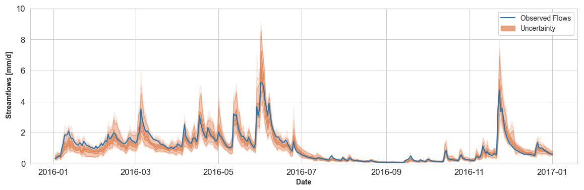
Figure 3 Example randomly selected for a catchment (station code K287191001 at Giroux with 756 km²) a catchment between 1 January 2016 and 1 January 2017 comprising both high- and low-flow events. Uncertainty estimates from QRF-local (orange) are plotted with the observed flows (blue). The orange line represents the median of uncertainty estimates, while darker orange shades indicate regions of higher probability (25 % and 75 % quantiles). Lighter regions indicate low probability quantiles (5 % and 95 % in addition to 2.5 % and 97.5 % quantiles).

4 Results

In this section, we compare each QRF variant according to its performance during the testing period. We investigate flow ranges in which multi-site learning is preferable, and we explore the importance of including catchment descriptors for regional QRFs. The results for the K-NN approach can be found in Appendix B. Figure 3 illustrates the uncertainty estimates of QRF-local for a randomly selected catchment.

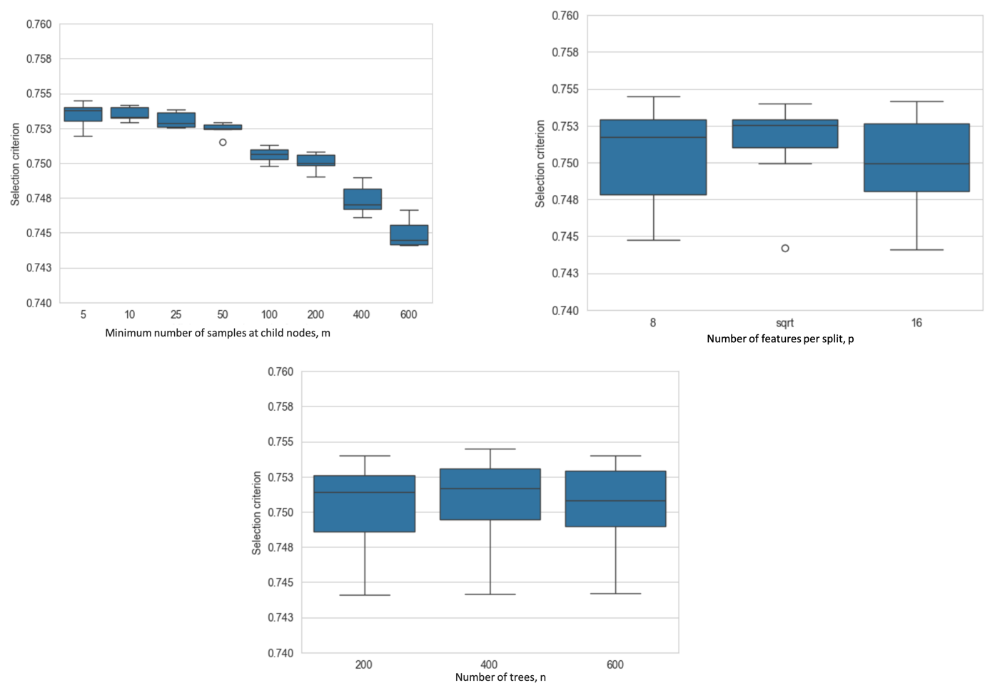
Figure 4 Hyperparameters optimization results for QRF-national. The selection criterion is the median hyperparameter criterion with equal contribution of the alpha score and CRPSS across the catchments of the study.

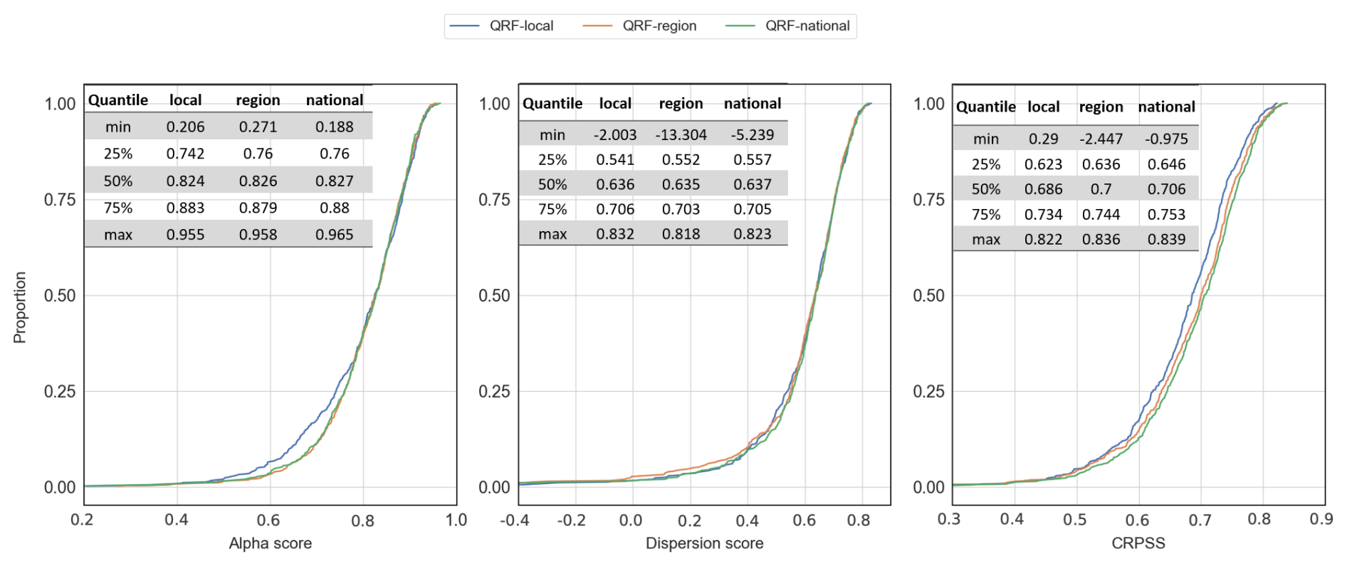
Figure 5 CDF of distributional metrics across the 564 catchments for the QRF variants in the study. Curves that are closer to the right of the plots indicate better performance. The blue line represents the performance of QRF-local, orange represents QRF-region, and green represents QRF-national.

4.1 Hyperparameter tuning

We conducted a hyperparameter grid search for each QRF variant using an equal contribution of the alpha score and CRPSS $\left(\frac{\mathit{\alpha }+\mathrm{CRPSS}}{\mathrm{2}}\right)$ as mentioned in Sect. 2.7. Figure 4 shows the hyperparameter tuning procedure for QRF-national's three hyperparameters: the minimum number of samples at child nodes, the maximum number of candidate variables to use for splitting at each tree node, and the size of the forest (number of trees). We aim to obtain a single set of hyperparameters, and the selection criterion is based on the median of the alpha score and CRPSS across all catchments of the study. Each subplot illustrates how the selection criterion varies with the hyperparameter under consideration, while the variability reflects the influence of the remaining hyperparameters. This allows to assess the sensitivity of the QRF-national to each hyperparameter during the optimisation process. Overall, the performance of QRF was most sensitive to the minimum number of samples at child nodes. QRF was trained with minimum number of samples at child nodes ranging from 5 to 600 data points.

It is notable that best results were recorded for lower values of the minimum samples at leaf nodes. The improvement slows for values lower than 25. As such, a minimum sample at leaf nodes of 10 is selected. Overall, QRF was found to be fairly insensitive to the number of candidate predictors used for splitting at each node. By default, the quantile-forest library uses the integer value of the square root (sqrt) of the total number of predictors for this parameter. With 31 total predictors for QRF-national, 6 would be the default. Figure 4 shows that using the default value of the square root was slightly better. For the number of trees parameter, a forest with more trees will generally be more skillful than one with fewer trees, as it can fit on the nuances of the training set, and there is a point when the rate of improvement with more trees is negligible, as noted in Oshiro et al. (2012) and Breiman (2001). Most of the boxplot ranges overlap, and the results appear to be relatively insensitive to this QRF parameter over the range considered.. For the experimented values, Fig. 4 shows that a number of 400 trees allows for slightly better performances. We selected hyperparameters for the other QRF variants using a more specific basis: per catchment for QRF-local and per region for QRF-region. One can expect that catchment specific hyperparameter tuning might help model performance. The distribution of the selected hyperparameters for QRF-local and-region is provided in Appendix D, as mentioned in Sect. 2.7.

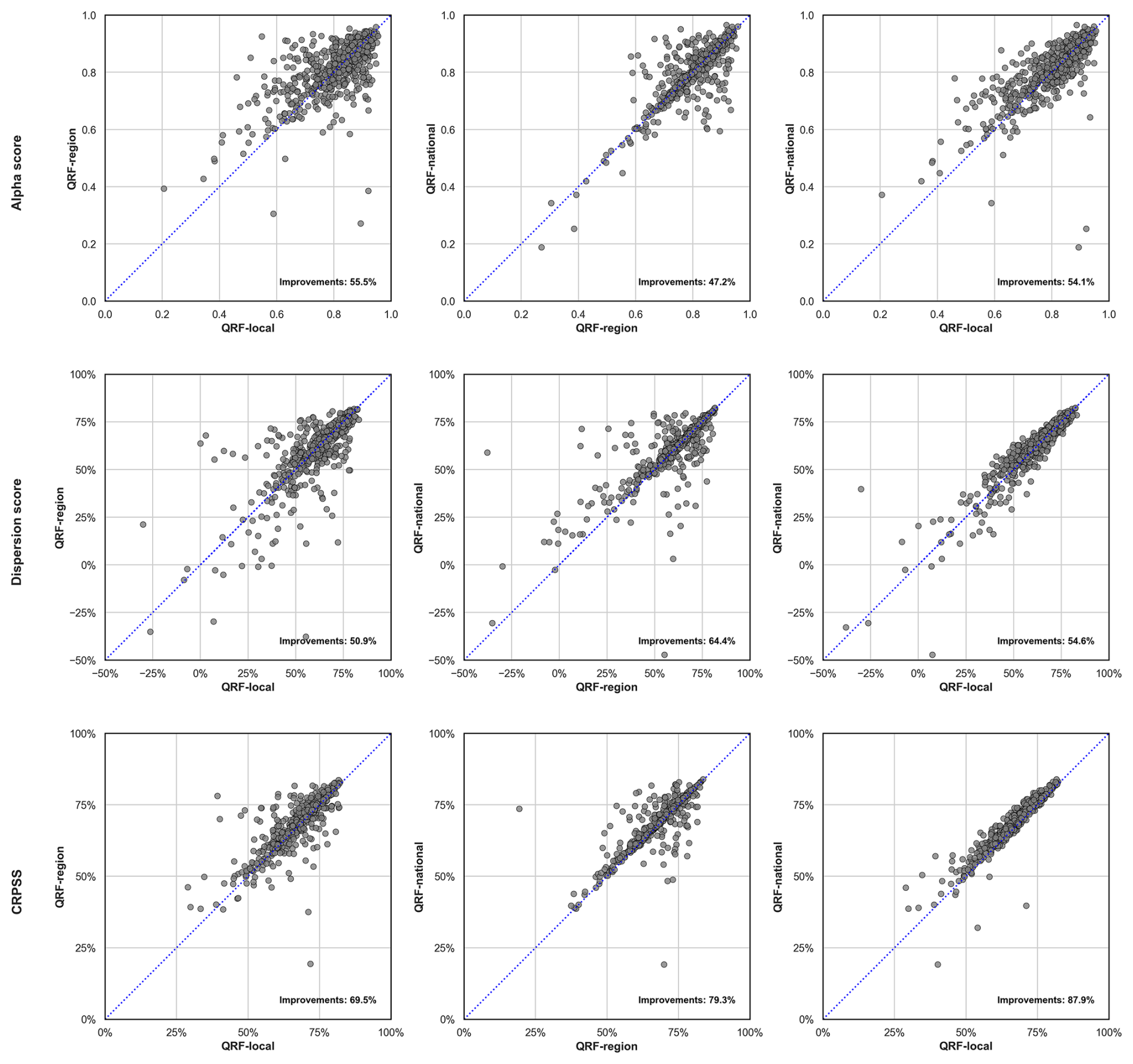
Figure 6 Comparative plots between QRF variants in the study during the testing period. The first row shows the alpha score, the second row shows dispersion, and the third row shows CRPSS. The first column compares metric values for QRF-local vs. QRF-region, the second column for QRF-national vs. QRF-region, and the third column for QRF-national vs. QRF-region

4.2 Alpha score, Dispersion score, and CRPSS

We first present our results with distributional metrics in Fig. 5, which shows the cumulative distribution of reliability, sharpness, and CRPSS for the 564 catchments of the study. QRF-region and QRF-national slightly improve reliability compared to QRF-local. However, multi-site learning does not yield better alpha scores for well-calibrated stations with QRF-local. Figure 6 shows a direct comparison of the proposed variants and indicates that improvements were most noticeable for catchments where QRF-local provided low reliability, i.e., 25 % of the basins with the lowest alpha scores (the 25 % quantiles of the alpha score were 0.742 for QRF-local and 0.76 and 0.76 for QRF-region and QRF-national, respectively). In terms of sharpness, the different QRF variants performed similarly, while multi-site setups significantly improve CRPSS values. Among the QRF variants, QRF-national generally outperformed QRF-local, improving CRPSS by approximately 2 %, except in the case of four catchments, where QRF-local performed significantly better. Additionally, QRF-region improved CRPSS for 69 % of the catchments compared to QRF-local, while QRF-national showed improvements in 88 % of the catchments. Overall, the improvements are less apparent for reliability, but multi-site QRFs seem to improve performance for catchments with initially limited reliability in the local setup. As highlighted in Sect. 3 CRPSS improvements combine both reliability or sharpness. Given that the sharpness metric was nearly identical across the QRF variants in the study, we suspect that the CRPSS improvements are mainly due to improvements in reliability. This is noteworthy, as the objective of probabilistic predictions is to improve reliability prior to enhancing sharpness (Gneiting et al., 2007).

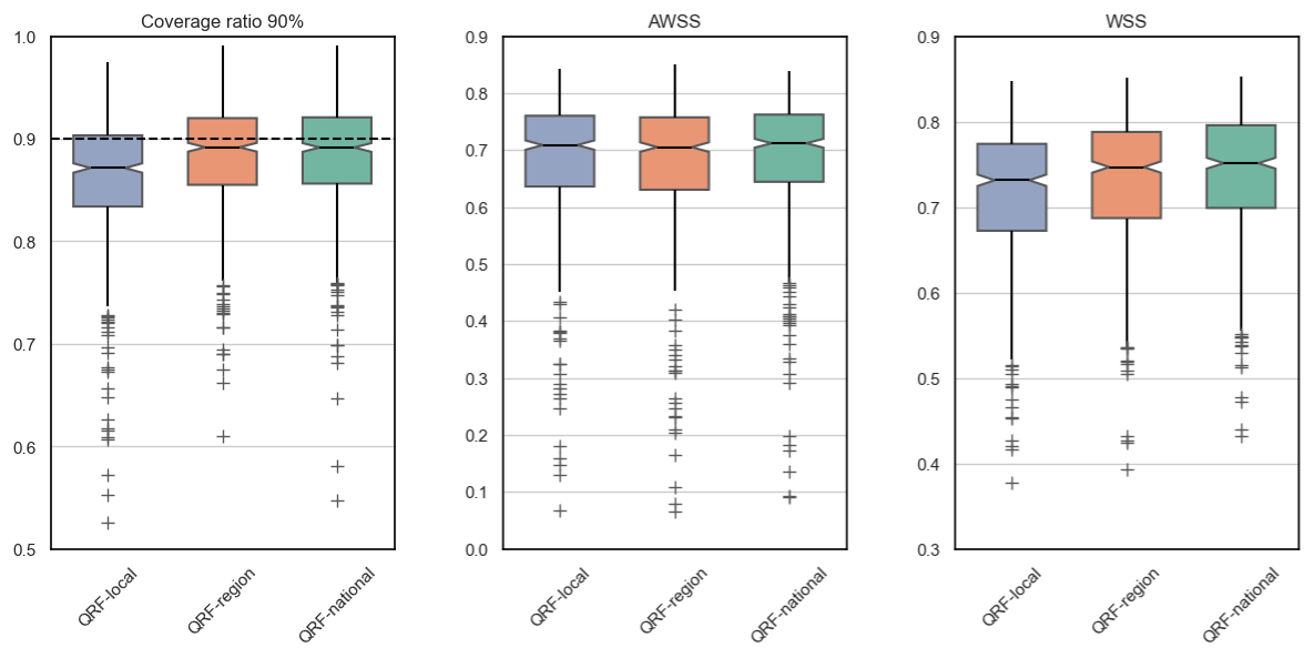
Figure 7 Box plots of 90 % interval-based metrics across the 564 catchments of the study. Blue indicates the performance of QRF-local, orange indicates QRF-region, and green indicates QRF-national.

4.3 Interval metrics

We now consider the 90 % interval metrics. Figure 7 represents the box plots across the 564 catchments of the study for coverage ratio, average interval width, and Winkler skill scores. The multi-site learning setup was beneficial for QRF and improved the reliability of the predictive intervals. For instance, the median coverage ratios were set at 0.87, 0.89, and 0.89 for QRF-local, QRF-region, and QRF-national, respectively. Similar to the alpha score, the improvements in the multi-site QRF variants are most noticeable for stations with low reliability in the local approach. As shown in Fig. 7, prediction intervals from multi-site QRFs over-cover observed streamflows (coverage ratio greater than 0.9) for certain catchments. While not optimal, this is a preferable outcome compared to the local approach, where uncertainty intervals more frequently miss the observed streamflows and tends to underestimate uncertainty in some catchments. The improvements are also observed for Winkler skill score, where QRF-national provided the best results. The average interval width was similar for all the variants in the study, further indicating that improvements in multi-site learning in the case of QRF mainly relate to reliability. For the sake of completeness, we include interval metrics for the 95 % predictive uncertainty interval in Appendix F, as the conclusions remain the same.

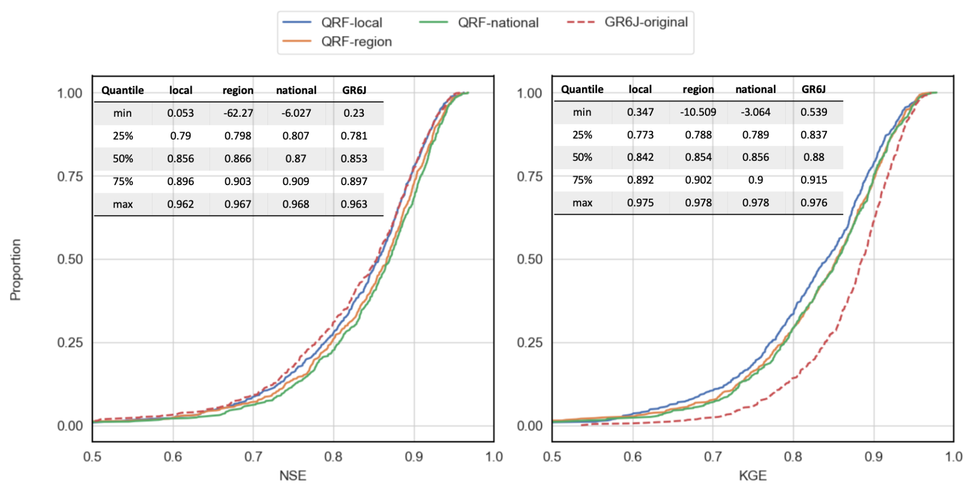
Figure 8 CDF of deterministic metrics across the 564 catchments for the QRF variants during the testing period. Curves that are closer to the right of the plots indicate better performance. The blue line represents the performance of mean uncertainty estimates for QRF-local, orange for QRF-region, green for QRF-national, while red represents the performance of raw GR6J predictions.

4.4 Deterministic metrics

Figure 8 shows the cumulative distribution function for the deterministic metrics of Nash–Sutcliffe efficiency (NSE) and Kling–Gupta efficiency (KGE) scores for mean predictions. Multi-site learning improves NSE for most catchments, but for KGE, improvements are most apparent when the local approach yields low KGE values. For example, when investigating catchments at the lower 25 % percentile, QRF-region and QRF-national improved the median KGE by 6 %. However, for catchments where QRF-local provided decent KGE scores (top 25 % performers), multi-site setups yielded similar scores to a single-basin approach. This would highlight the equalizing effects of multi-site learning for QRF, as it is most impactful for catchments with limited performance in the single-basin post-processing.

Figure 8 also provides deterministic metrics for the uncorrected GR6J model predictions. The figure highlights that the proposed QRF methods can improve hydrological deterministic predictions, especially for NSE. For example, QRF-national produced better NSE performance compared to GR6J predictions (0.87 vs 0.86 in median NSE) and for 75 % of the study’s catchments. Overall, QRF variants had better NSE for the majority of the catchments. For KGE, the uncorrected GR6J estimates outperform all tested QRF approaches.

We argue that these results show: (i) the ability of QRF in its multi-site setup to identify and transfer useful information from neighbouring catchments; (ii) although the improvements relate to both deterministic and uncertainty predictions, they are most significant for coverage ratio, CRPSS, WSS, NSE, and KGE. Building on these findings, we investigated whether these benefits were more pronounced under specific hydrological conditions.

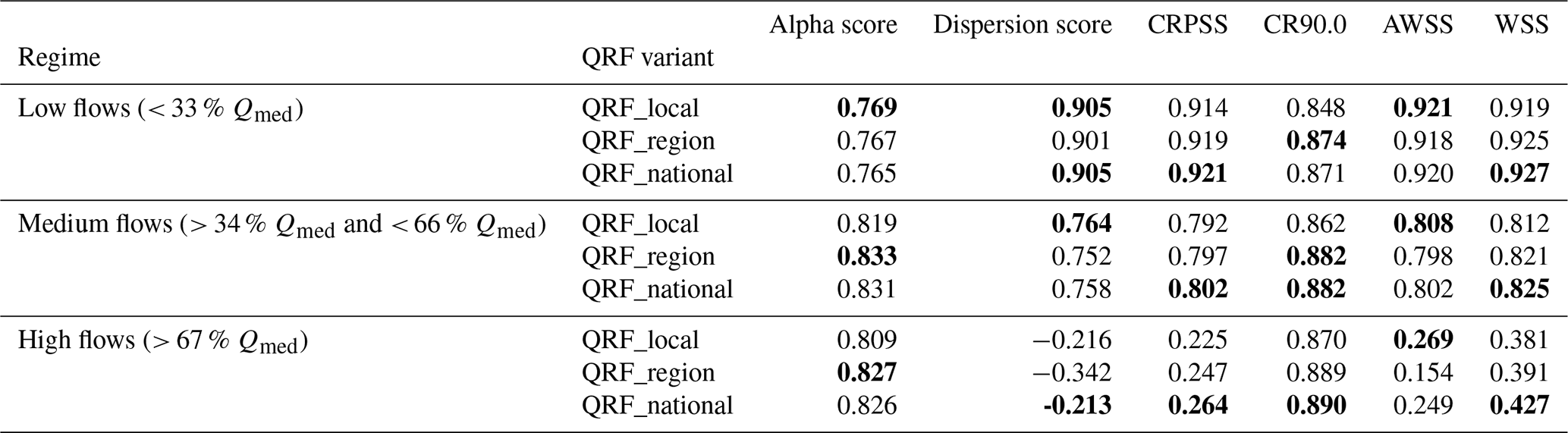
Table 4 Summary of average metrics for different QRF methods across the 564 catchments of the study. Three flow ranges are included: high, medium, and low simulated flows. The bold numbers indicate better performance in each group.

4.5 How do QRF uncertainty estimates perform for different flow ranges?

Here, we aim to understand how the proposed QRF approaches perform across different flow ranges. Table 4 summarizes the average values of the alpha, dispersion, CRPSS, and interval scores for three flow groups: high (> 67 % Q_med), medium (> 34 % Q_med and < 66 % Q_med), and low flows (< 33 % Q_med).

Performances were stratified based on the median values of the uncertainty distributions. Under low-flow conditions, the scores are similar, especially alpha and dispersion scores. But for higher simulated flows, multi-site QRFs provide better reliability (alpha score and coverage ratio) and better overall performance (CRPSS and WSS). Although QRF-local was able to provide narrower interval widths, especially for higher flows, it had lower reliability compared to multi-site QRFs. QRF-region and QRF-national adapt to higher-flow ranges by providing wider uncertainty estimates and enable better reliability and conditionality, as reflected in the improved CRPSS and Winkler scores.

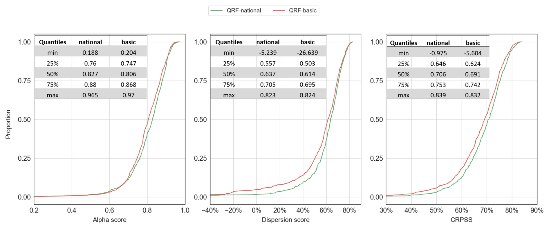
Figure 9 Distributional metrics across the 564 catchments for the QRF variants in the study. Curves that are closer to the right of the plots indicate better performance. The red line represents the performance of QRF-basic and green represents QRF-national.

4.6 Impact of static descriptors

To understand the impact of static catchment descriptors, Fig. 9 illustrates the distributional metrics for QRF-national and QRF-basic. QRF-basic is a multi-site QRF trained across all catchments of the study and using the same features as for QRF-local (no static features). Notable differences between the two variants are observed: in terms of reliability (median 0.827 vs. 0.806 across all catchments), sharpness (0.637 vs. 0.614), and CRPSS (0.706 vs. 0.691). Largest differences are observed for CRPSS, as QRF-national was better for 80 % of the stations of the study. Furthermore, Fig. F2 in Appendix F shows that QRF-basic had very similar CRPSS values as for QRF-local. These results suggest that the performance improvements in multi-site QRF models are not solely due to the inclusion of hydrological diversity in the training data. Static catchment descriptors play a significant role, and the selection of informative static features appears to be critical for effective multi-site QRF implementations.

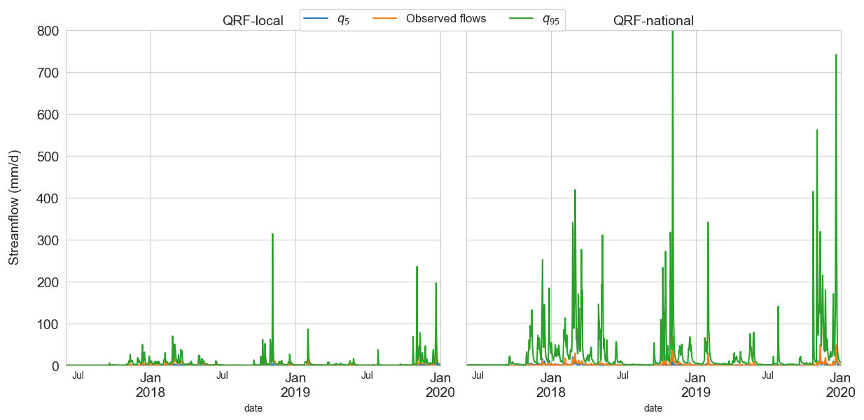
Figure 10 Example uncertainty estimates for a Mediterranean catchment (Solenzara River at Sari-Solenzara [Canniciu]; station Y960000102) from QRF-local (left) and QRF-national (right), covering the period from July 2017 to January 2020. The estimated 5 % quantile is shown in blue, and the 95 % quantile in green. The QRF-national model noticeably overestimates the upper (95 %) uncertainty quantile.

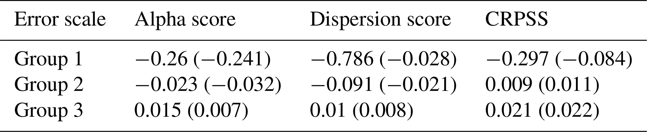
Table 5 Average and median (shown in parentheses) differences between QRF-local and QRF-national models across distributional metrics, evaluated across different error scale groups. For catchments with extreme error variability (Group 1), QRF-national model degrades the quality of uncertainty estimates.

4.7 Sensitivity to scale (potential for improving the performance of QRF-national)

Following the results of the previous section, we found that multi-site learning can significantly degrade the performance for four cases across distinct hydrological regions; an example of such catchments is presented in Fig. 10. To investigate this, Table 5 presents the differences in performance (alpha score and CRPSS) between QRF-national and QRF-local based on the variability of errors ϵ_t for three groups: group 1 is characterized by important error variability (> 1.5), group 2 also has important error variability but to a lesser degree (0.77 < and  < 1.5), and group 3 (< 0.77) which can be seen as having normal variability. Values 1.5 and 0.77 are the 99 % and 90 % quantiles of the interquartile range used to standardize the errors ϵ_t. QRF-national performed poorly for catchments with significant variations in the target variable, with notable decreases in reliability and CRPSS compared to a single-basin approach. These results highlight that robust standardization of input variables and errors is key to delivering meaningful multi-site QRFs, since this enables the algorithm to find analogs from locally calibrated hydrological model inputs. Furthermore, the aforementioned scale discrepancies occurred specifically for catchments characterized by frequent zero values in simulated and observed streamflows. This can be problematic when using logarithmic relative hydrological errors. Figure 10 illustrates QRF-local and QRF-national predictions for the 5 % and 95 % quantiles alongside observed flows for the Y960000102 catchment. Clearly, QRF-national overestimates the upper quantile. The local approach thus yields better results, since the error dynamics of this catchment are unconventional compared to the other catchments of the study.

5 Discussion

5.1 When and where is it preferable to use a multi-site learning setup?

Although training QRF on local data yields good uncertainty estimates, as discussed in previous studies (Taillardat et al., 2016; Zhang et al., 2023), using a multi-site setup can slightly improve QRF performance. Our results indicate that the best improvements are achieved with QRF-national, which includes all 564 catchments of the study. The improvements mainly concern (i) catchments where local information is not sufficient (i.e., limited QRF-local performance), (ii) CRPSS and WSS scores for nearly all catchments, and (iii) periods of higher flows.

The results presented in Sect. 4 indicate that multi-site learning improves the performance of QRF models, and that larger models yield better uncertainty estimates (QRF-national > QRF-region > QRF-local). We find this result interesting, since one might argue that regional models in the QRF-region approach provide an equilibrium in spatial variability by aggregating similar catchments and, possibly, similar error dynamics (Johnson et al., 2023). Such an approach confines the QRF analog search to specific hydrological regions, without extending the search to the entire study area. QRF-national, however, is not constrained by the predefined hydro-climatological regions. Region indicators are included as input features for QRF-national, and the algorithm is trained to find analogous events using these indicators, but is not strictly limited by them. Spatial variability appears to be beneficial for QRF, provided that appropriate catchment descriptors are used, and incorporating explicit measures of catchment similarity could further improve multi-site learning with QRF (Hashemi et al., 2022; Kratzert et al., 2024).

Most improvements are noted for high and medium flows. QRF-national provided a better alpha score, i.e., reliability for 60 % of the catchments during high and medium flows compared to QRF-local, but performance was identical for low flows. As highlighted in Bertola et al. (2023) and Auer et al. (2024), high flows are generally more difficult to predict and some high-flow events cannot be predicted exclusively from local historical data. QRF makes use of information from neighboring catchments to provide uncertainty estimates for these events that can be more challenging to predict. Local information seems to be sufficient to characterize low-flow events.

The provided analyses highlighted a limitation of the multi-site QRFs which concerns catchments characterized by frequent zero flow values. Modelling hydrological model errors of ephemeral catchments is generally challenging (McInerney et al., 2019; Li et al., 2016), particularly with the use of a log-based error transformation. Figure 10 shows that multi-site learning can degrade the predictions for ephemeral catchments as uncertainties are overestimated. Although we have added the δ offset parameter, the use of an alternative transformation that is better suited to zero flow values (e.g., a Box–Cox transformation) could better stabilize hydrological errors used to train the QRF models for ephemeral catchments. Another solution could be the treatment of such catchments separately when training multi-site QRF. As showed in Fig. 10, QRF-local better managed the case of zero flow values. In the literature, other approaches (Hashemi et al., 2022; Fang et al., 2024) use adapted catchment groupings based on clustering approaches grouping homogeneous catchments. The use the number of zero flow values or the clusters as inputs to QRF can allow QRF to better distinguish catchments characterized by this issue.

Also, we expected that the proposed variants would also improve KGE as was observed in the previous studies of (Zhang et al., 2023; Shen et al., 2022; Magni et al., 2023). For example, Magni et al. (2023) used a closely related deterministic RF framework for hydrological error correction and found that the hybrid RF approach boosted streamflow predictions from a median of −0.03 to 0.51. Here, the post-processing was not beneficial for KGE performances, and we suggest that this can be attributed to how QRF hyperparameters were selected. The used selection criterion in this study aims to maximize the probabilistic performances of reliability and sharpness of the uncertainty estimates. While for the aforementioned studies, the RF post-processor was optimized specifically for deterministic error correction.

5.2 What is the importance of meaningful catchment attributes?

We showed in Fig. 9 that the improvements in QRF-national depend on the use of static descriptors. A nation-wide QRF variant with no catchment attributes (identical input descriptors to the local variant) performed worse than a classic single-catchment QRF. This indicates that increasing hydrological diversity and lumping more catchment data are not the primary drivers of performance improvements. The information shared within a multi-site setup is best used by the QRF algorithm in conjunction with quality catchment descriptors. This would enable better uncertainty characterization and improved analog searches in similar catchments. The catchment descriptors used are readily available in the CAMELS-FR and other CAMELS datasets, making the use of such descriptors straightforward. Furthermore, a globally parametrized QRF post-processor is able to extend its uncertainty estimates into ungauged catchments. Magni et al. (2023) found that RF is able to learn global mappings and improve deterministic estimates in poorly gauged and ungauged basins. Similar improvements could be obtained in an uncertainty estimation at ungauged catchments context, if appropriate catchment descriptors that do not rely on observed streamflows are selected.

5.3 Multi-site QRF for extrapolation of hydrological uncertainties

We used a large sample dataset (CAMELS-FR) to train the QRF model, and many practical hydrological applications can be interested in applying QRF post-processing to catchments not included in the training set. Our study demonstrates the ability of the QRF model to make use of hydrological information from neighbouring catchments to improve uncertainty estimates. Building on this finding, we suggest that applying a multi-site QRF, supported by appropriate catchment descriptors, to catchments outside the training set is likely to yield improved uncertainty estimates compared to a QRF model trained with single catchment data. However, the quality of these estimates remains unexplored, as the generalizability of multi-site QRF variants would depend on the similarity between hydrological model errors between the training catchments and the target regions to which uncertainty estimates are extrapolated. A spatio-temporal cross-validation experiment (Fang et al., 2024) that splits the training and testing by catchments and time periods can be used to understand the flexibility of multi-site QRF post-processing. Also, the proposed framework can be adapted for a prediction at ungauged basins. to explore this extension, the main practical difficulty lies in obtaining consistent hydrological model states for ungauged catchments, and to adapt the significant additional uncertainty usually associated with such settings (Razavi and Coulibaly, 2013; Oudin et al., 2008; Bourgin et al., 2015). If this can be properly handled, the proposed QRF multi-site variants could provide meaningful uncertainty estimates in the context of uncertainty estimation for ungauged catchments. A comparison to LSTM based post-processing techniques would be also interesting, as LSTMs perform well in ungauged basin setting (Kratzert et al., 2018).

5.4 On model complexity and computational time

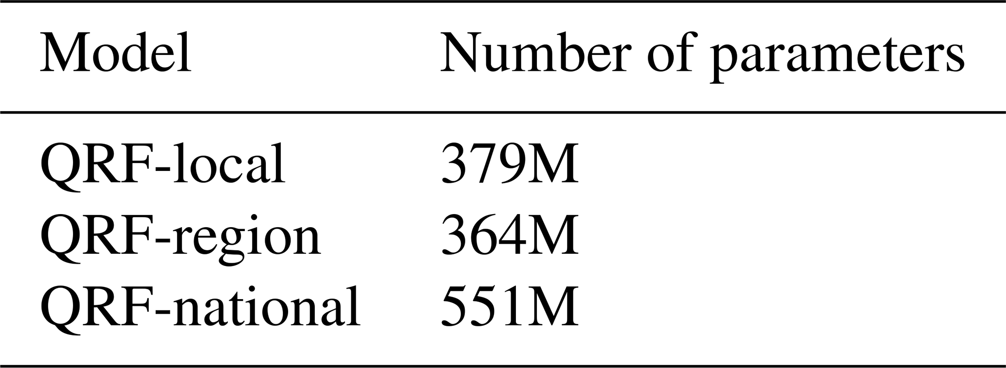
Table 6 presents the number of parameters for each QRF variant, calculated as the product of the number of trees and the parameters of each tree (e.g., split thresholds, used input features). QRF-region and QRF-local exhibit a similar number of parameters, despite QRF-region providing better uncertainty estimates. In contrast, QRF-national shows a 47 % increase in model complexity. This suggests that the performance gains of QRF-national come at the expense of increased computational cost which can be a drawback, especially since QRF stores not only the tree parameters but also samples used for training.

Table 6 Cumulative number of parameters across all models.

RF-based algorithms are CPU-intensive and suffer from memory voracity, especially for larger datasets Taillardat and Mestre (2020). In the case of our study, we had no difficulty fitting QRF-local and QRF-region with an Intel(R) Core(TM) i7-4770 CPU (3.40 GHz) and 16 GBs of memory. However, because of memory issues, we trained QRF-national on Jean-Zay HPC, where a single node with two CPUs (at 2.5 GHz) and 128 GBs of memory was sufficient. With this configuration, it takes on average 25 min to fit QRF-national with a single parameter. While training time is longer for multi-site settings, inference/prediction times are very similar to those of QRF-local.

6 Conclusions

In this study, we investigated the added value of multi-site learning with a hydrologically informed quantile random forest (QRF) post-processor across a large set of 564 French catchments. Three training setups were proposed – local, regional, and national – which we evaluated with different probabilistic metrics and across various hydrometeorological conditions. Based on reliability, sharpness, and overall metrics, our results indicate that multi-site learning improves QRF uncertainty estimates, with notable enhancements; (i) for overall metrics (CRPSS and WSS) and deterministic metrics (NSE and KGE) (ii) at stations where the local approach provided unreliable uncertainty estimates; and (iii) for high and medium flows, where predictions can be more challenging. These findings corroborate previous studies (Fang et al., 2024; Bertola et al., 2023; Auer et al., 2024) that found that high-flow events can have similar characteristics in neighbouring catchments. These results suggest that the QRF algorithm in its regional extensions can leverage data from neighbouring catchments to improve its uncertainty estimates; this is particularly advantageous given the off-the-shelf use of available catchment descriptors and the similarity of the learning process between local and regional variants. Additionally, the selection of representative and quality catchment attributes and static features is necessary to achieve the aforementioned improvements. We also found that using a single QRF post-processor for all catchments in the study (QRF-national) provided the best probabilistic predictions, which might indicate that the larger the model the better the uncertainty estimates with QRF. But QRF-national can yield erroneous uncertainty estimates for catchments with significant scale variations in the errors. We argue that this is mainly due to the use of logarithmic transformation of relative errors, which strongly influences hydrological error dynamics at such stations. The use of other transformations and experimenting with other catchments groupings (Hashemi et al., 2022) could solve this issue. In addition, larger models are associated with higher computational costs, with increased complexity, and with a larger number of parameters. This is particularly relevant for QRF, as RF-based algorithms are known for their intensive memory use. However, some solutions include the use of GPU-accelerated QRFs (Raschka et al., 2020).

We acknowledge certain limitations related to model-dependent artifacts. In this study, we were able to test QRF variants only using the GR6J hydrological model, as it was the only model for which simulations were available. However, the proposed framework is flexible and can be extended to other hydrological models and states. A comparison with other error models is also an attractive option, this includes standard Autoregressive models, and LSTM based error modelling. These findings highlight the performance enhancements of regional hydrologically informed QRF post-processing, and we aim to explore further in future studies the merits of the proposed QRF framework in both forecasting applications and prediction at ungauged basins.

Appendix A: Overview

The Appendix is structured as follows: Appendix B compares the overall performance of K-Nearest Neighbors model against QRF-local. Appendix C investigates the power transformation used to calibrate the hydrological model GR6J. Appendix D provides the distribution of the selected hyperparameters for QRF-local and QRF-region variants, Appendix E details the used assessment criteria used to compare the uncertainty quantification approaches of the study. Finally, Appendix E provides additional results that complement the main paper.

Appendix B: K-Nearest Neighbors model as benchmark

B1 K-Nearest Neighbours algorithm

We used a naive k-nearest neighbors approach as a benchmark. The k-nearest neighbors (K-NN) algorithm is a non-parametric method that makes predictions based on the closest historical examples in the feature space. In hydrology, it is often used to estimate streamflow by averaging the outputs of the k most analogous conditions. Here analogs were used to estimate uncertainty, on a local basis. Table B1 presents the hyperparameters used for the K-NN algorithm, while Table B2 compares the approaches K-NN and QRF-local. Average and median (between parentheses) across the catchments of the study, including distributional, interval and deterministic metrics.

Table B1 Hyperparameters Set Optimized for K-NN approach.

B2 K-Nearest Neighbours and QRF-local comparison

Table B2 compares the average and median performance metrics of QRF-local and K-NN across the 564 catchments. Overall, QRF-local consistently outperforms K-NN across all evaluated metrics. It achieves higher alpha scores, improved dispersion scores, and better CRPSS values, indicating both more reliable and more skillful probabilistic predictions. These results suggest that QRF-local leverages dynamic input features more effectively than the simpler K-NN approach.

Table B2 Average performance scores across the 564 catchments for QRF-local and K-NN. Median scores are shown in parentheses. Bold values indicate better performance for each metric.

Appendix C: Prior transformations on streamflow

The power transformations are applied to the target variable – both observed and simulated streamflows – before calculating the associated KGE criteria (Eq. C1). For example square root transformation aim at increasing the weight of errors for specific hydrological regimes. The use of streamflow transformations for model calibration is further investigated in the recent study of Thirel et al. (2024)

$$\begin{array}{}\text{(C1)}& {\displaystyle }\mathrm{\text{KGE}}(Q_{\text{obs}}^{\mathrm{p}},Q_{\text{prd}}^{\mathrm{p}})=\mathrm{1}-\sqrt{(r-\mathrm{1}{)}^{\mathrm{2}}+(\mathit{\alpha }-\mathrm{1}{)}^{\mathrm{2}}+(\mathit{\beta }-\mathrm{1}{)}^{\mathrm{2}}}\text{(C2)}& {\displaystyle }r={\displaystyle \frac{\text{Cov}(Q_{\text{obs}}^{\mathrm{p}},Q_{\text{prd}}^{\mathrm{p}})}{{\mathit{\sigma }}_{\text{obs}}{\mathit{\sigma }}_{\text{prd}}}}\text{(C3)}& {\displaystyle }\mathit{\alpha }={\displaystyle \frac{{\mathit{\sigma }}_{\text{prd}}}{{\mathit{\sigma }}_{\text{obs}}}}\text{(C4)}& {\displaystyle }\mathit{\beta }={\displaystyle \frac{{\mathit{\mu }}_{\text{prd}}}{{\mathit{\mu }}_{\text{obs}}}}\end{array}$$

Where: r is the Pearson correlation coefficient, α is the variability ratio, β is the bias ratio. μ and σ represents the mean and standard deviation of the transformed streamflow time series.

Appendix D: Distribution of QRF hyperparameters for QRF-local and -region

Figures D1 and D2 show the distribution of hyperparameters for QRF-local and QRF-region, respectively. Unlike the national approach, which uses a single set of hyperparameters, QRF-local assigns one set per catchment, while QRF-region uses one set per region. Overall, hyperparameters vary across catchments and regions. Important variability is observed for the minimum number of samples at child nodes, which which affects trees depth. The values of this hyperparameter were mostly skewed toward lower ranges for both QRF-local and QRF-region. The response of QRF-local to the other hyperparameters was less discriminative. For QRF-local, the selected values for the number of trees and features per split remained largely consistent across the values tested. For QRF-region, 200 trees were most often selected, while 8 features and the default square root (6 features per split) were the most frequent optimal value for the number of features per split hyperparameter.

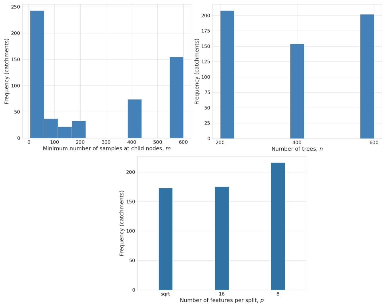
Figure D1 Distribution of the selected hyperparameters for QRF-local across the catchements of the study. The hyperparameters are: (i) The number of trees n, (ii) The minimum number of samples at child nodes m, and (iii) The number of features per split, p.

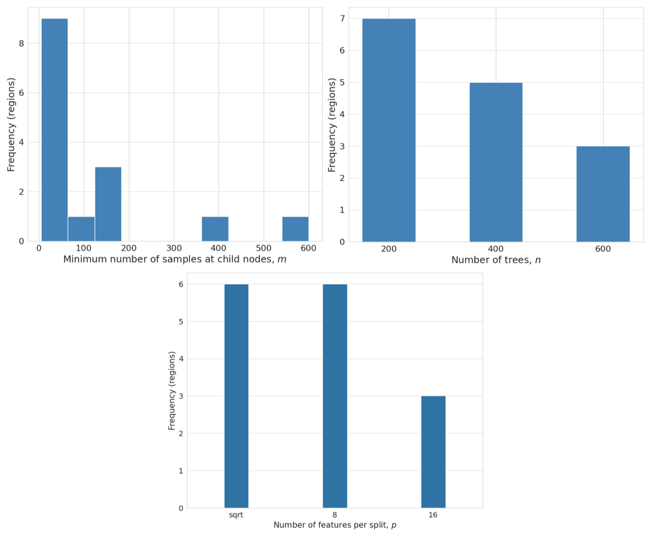
Figure D2 Distribution of the selected hyperparameters for QRF-region across the hydroclimatological catchment groups used in the study. The hyperparameters are: (i) The number of trees n, (ii) The minimum number of samples at child nodes m, and (iii) The number of features per split, p.

Appendix E: Assessment criteria

E1 Continuous ranked probability score

Given a univariate predictive distribution F and a corresponding realization y, the continuous ranked probability score (CRPS) is defined as:

$$\begin{array}{}\text{(E1)}& \text{CRPS}(F,y)=\underset{-\mathrm{\infty }}{\overset{+\mathrm{\infty }}{\int }}\left(F\right(u)-H(u-y){)}^{\mathrm{2}}\mathrm{d}u,\end{array}$$

where H is the Heaviside function such that $H(u-y)=\mathrm{1}$ if u≥y and 0 otherwise. In this study, the probabilistic predictions are in the form of draws distributions; hence, Eq. (E1) has to be discretized for computation. We apply the method which is implemented in the function “CRPS_FROM_ECDF” from the Python package EvalHyd (Hallouin et al., 2024). The CRPS is negatively oriented, meaning that smaller values are better.

E2 Skill score

The performance of predictions can be more easily compared with that of a reference prediction skill scores. Skill scores (SS) are used to assess the relative quality of two predictions. They are generally defined as: SS it is generally defined as:

$$\begin{array}{}\text{(E2)}& \text{SS}=\mathrm{1}-{\displaystyle \frac{\stackrel{\mathrm{‾}}{S}}{\stackrel{\mathrm{‾}}{S_{\text{ref}}}}}\end{array}$$

where $\stackrel{\mathrm{‾}}{S}$ and $\stackrel{\mathrm{‾}}{S_{\text{ref}}}$ are the scores of predictions from the model to evaluate and the reference model, respectively. Climatology is commonly used as a reference. In this study, we consider climatological distributions of observed streamflows. It has been estimated as the empirical distribution of discharges across the training periods (P1).

E3 Alpha score

Given a univariate forecast distribution F_t and a corresponding realization y_t, the p value is $F_{\mathrm{t}}\left(x_{\mathrm{t}}\right)=p(Y_{\mathrm{t}}\le y_{\mathrm{t}})$ and the alpha score is defined as:

$$\begin{array}{}\text{(E3)}& {\mathit{\alpha }}_y^{\prime }={\displaystyle \frac{\mathrm{1}}{N_y}}\sum _{i=\mathrm{1}}^{N_y}\left|p_{y\left(i\right)}-p_{y\left(i\right)}^{\left(th\right)}\right|\end{array}$$

where $p_y^{\left(i\right)}$ and p_y(i)^(th) are the ith observed and theoretical p values of y_t values. N_y is the number of y_t values. The alpha score takes values between 0 and 1. It is positively oriented, with scores close to 1 reflecting perfect reliability.

The performance of streamflow forecasts can vary depending on the flow range considered (e.g., flood forecasting vs. drought forecasting). Bellier et al. (2017) suggest a forecast-based sample stratification for continuous scalar variables in order to consider the merits of streamflow forecasts on different ranges of flows. To ensure robust reliability estimates and prevent potential compensation effects, the alpha score was calculated separately for three distinct flow ranges: low, high, and average forecasted flows.

E4 Dispersion score

Sharpness is quantified with the skill score of the forecast CRPS of median forecasts relative to climatological streamflow distribution, in which CRPS median is defined as follows:

$$\begin{array}{}\text{(E4)}& {\text{CRPS}}_{\text{median}}\left(F\right)=\text{CRPS}(F,F_{\text{median}})\end{array}$$

where F_median is the median value of the distribution F. This is related to an interesting decomposition of the CRPS proposed in the PhD thesis of Bontron (2004)

E5 Coverage ratio

Given a predictive interval [L_t,U_t] at a confidence level 1−α and a corresponding observation y_t, the coverage ratio (CR) is defined as:

$$\begin{array}{}\text{(E5)}& \text{CR}={\displaystyle \frac{\mathrm{1}}{N}}\sum _{t=\mathrm{1}}^N\mathbf{1}\mathit{\{}{y}_{\mathrm{t}}\in [L_{\mathrm{t}},U_{\mathrm{t}}\left]\mathit{\right\}},\end{array}$$

where 1{⋅} is the indicator function and N is the number of observations.

E6 Average width

The average width (AW) of the prediction intervals is given by:

$$\begin{array}{}\text{(E6)}& \text{AW}={\displaystyle \frac{\mathrm{1}}{N}}\sum _{t=\mathrm{1}}^N(U_{\mathrm{t}}-L_{\mathrm{t}}),\end{array}$$

quantifying the sharpness of the probabilistic forecasts.

E7 Winkler score

The Winkler score (WS) penalizes both miscoverage and interval width and is defined as:

$$\begin{array}{}\text{(E7)}& \begin{array}{rl}{\text{WS}}_{\mathrm{t}}=& (U_{\mathrm{t}}-L_{\mathrm{t}})+{\displaystyle \frac{\mathrm{2}}{\mathit{\alpha }}}(L_{\mathrm{t}}-y_{\mathrm{t}})\mathbf{1}\mathit{\{}{y}_{\mathrm{t}}<L_{\mathrm{t}}\mathit{\}}\\ & +{\displaystyle \frac{\mathrm{2}}{\mathit{\alpha }}}(y_{\mathrm{t}}-U_{\mathrm{t}})\mathbf{1}\mathit{\{}{y}_{\mathrm{t}}>U_{\mathrm{t}}\mathit{\}},\end{array}\end{array}$$

and the overall score is averaged over all observations: $\text{WS}=\frac{\mathrm{1}}{N}{\sum }_{t=\mathrm{1}}^N{\text{WS}}_{\mathrm{t}}$.

Appendix F: Results supplement

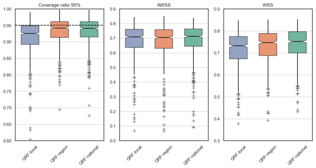
Figure F1 Box plots of 95 % interval-based metrics across the 564 catchments of the study. Blue for the performance of QRF-local, orange for QRF-region, and green for QRF-national.

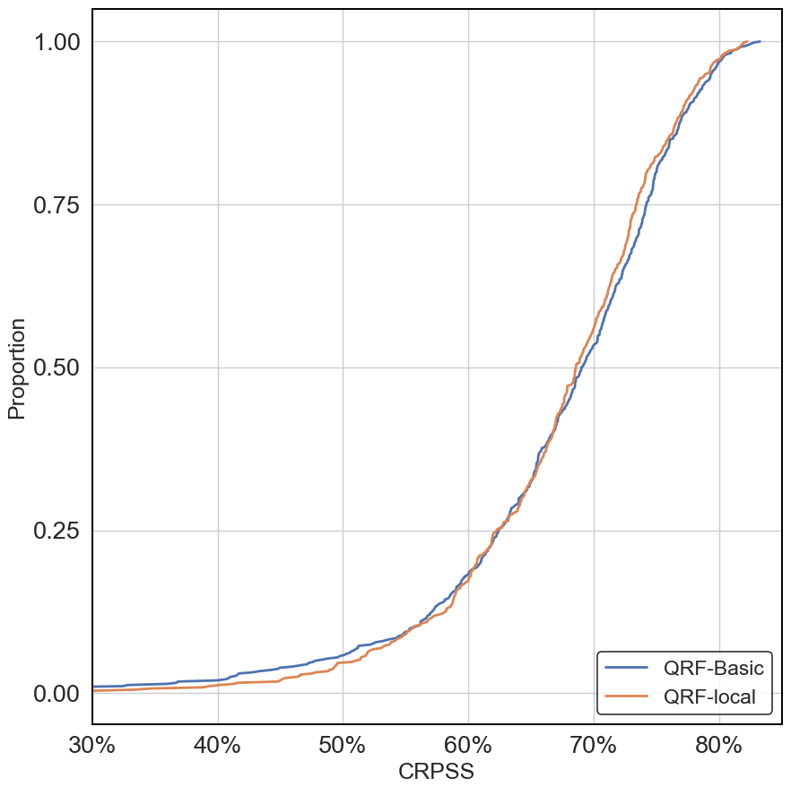
Figure F2 CRPSS metric across the 564 catchments. The blue line represents the performance of QRF-basic, orange represents QRF-local.