Testing discharge assimilation strategies to enhance short-range AI-based operational rainfall–runoff forecasts

Effective discharge forecasts are essential in operational hydrology. The accuracy of such forecasts, particularly in short lead times, is generally increased through the integration of recent measurements of observed discharge; commonly known as discharge assimilation (DA). Recent studies have demonstrated the effectiveness of deep learning (DL) approaches for rainfall–runoff (RR) modeling, particularly Long Short-Term Memory (LSTM) networks, outperforming traditional approaches. However, most of these studies do not include DA procedures, which may limit their operational forecast performance. This study suggests and evaluates three DA strategies that incorporate discharge from either recent discharge measurements or forecasts from a pre-trained rainfall–runoff model. The proposed strategies, based on a Multilayer Perceptron (MLP) as orchestrator, include: (1) the integration of recently observed discharges, (2) the integration of both recent discharge observations and pre-trained model forecasts, and (3) the post-processing of model forecast errors. Experiments are implemented using two large datasets, CAMELS-US and CAMELS-FR, and two established benchmark models (BM): the trained LSTM model from Kratzert et al. (2019) and the conceptual Sacramento Soil Moisture Accounting (SAC-SMA) model from Newman et al. (2017), covering both deep learning and conceptual RR simulation approaches. The considered lead times range from 1 to 7 d, covering both short- and mid-term horizons. The approaches are evaluated within two forecast frameworks: (1) perfect meteorological forecasts over the forecasting lead time and (2) ensemble meteorological forecasts. The two frameworks yield contrasting outcomes. When evaluated under the perfect forecast framework, the application of DA leads to substantial improvements in forecast performance, although the magnitude of these gains depends on the initial performance of the benchmark models and the forecasting lead time. Improvements are consistently significant for the SAC-SMA cases, while for the LSTM cases, gains are observed mainly for basins where the LSTM initially underperforms. However, the ensemble forecast evaluation yields unexpected results: the performance ranking of the tested models changes markedly compared to the perfect forecast framework. The LSTM model, in particular, appears penalized by the under-dispersion of its forecast ensembles. Although this underdispersion could be partly attributable to the underdispersion of the forecast archives tested, it persists even when the model is driven by the high spread climatology-based ensemble. This finding underscores the importance of ensuring reliable ensemble dispersion for the efficient operational deployment of AI-based hydrological forecasts.

1 Introduction

Discharge forecasting models are essential in operational hydrology, whether for water resource or related-risk management. Their importance is set to increase as climate-related threats intensify (Schiermeier, 2018; Philip et al., 2020; Rentschler et al., 2023). However, providing accurate discharge forecasts remains challenging due to the complexity of rainfall–runoff (RR) processes, model imperfections, and uncertainty in input data, particularly regarding the quality of weather forecasts.

Over decades, significant efforts have been made to address the challenges of hydrological modeling, leading to the development of various models and approaches. In the era of artificial intelligence (AI), notable advances have been achieved, with recent studies demonstrating the outstanding performance of deep learning models (DL) relative to traditional RR models (Kratzert et al., 2019; Husic et al., 2022). Commonly used DL architectures include multilayer perceptrons (MLPs) (Jeannin et al., 2021; Saint-Fleur et al., 2023), recurrent neural networks (RNNs) such as Long Short-Term Memory (LSTM) networks (Kratzert et al., 2018, 2019; Fang et al., 2021; Wunsch et al., 2021; Rahbar et al., 2022), and more recently, Transformers (Pölz et al., 2024). Nonetheless, most hydrological models in the literature are evaluated mainly under perfect weather scenarios, which may overestimate their performance in an operational forecasting framework. Although simulation models can be incorporated into forecasting systems, either as assimilable data or driven by forecasted forcings, their development frequently overlooks key components such as discharge assimilation, persistence analysis, and ensemble (probabilistic) assessment.

Persistence analysis, introduced by Kitanidis and Bras (1980), evaluates a model's performance relative to a naive baseline, which simply translates the current observation to the target lead time. This analysis, which serves as a relevant benchmark for assessing the predictive ability of models, is rarely considered in most hydrological modeling studies. Discharge assimilation (DA), on the other hand, which consists of dynamically providing real-time discharge data to a running forecast model, is essential in operational forecasting (Bourgin et al., 2014; Boucher et al., 2020; Piazzi et al., 2021). By ensuring regular updates of the model states, DA allows one to reduce the impact of uncertainties associated with meteorological forecasts and model structures, thus keeping the model aligned with evolving hydrological conditions. Several DA techniques exist, and their efficacy often depends on the reliability of the underlying model and/or the techniques used (Feng et al., 2020; Nearing et al., 2022; Yang et al., 2025). For direct DA strategies, the importance of DA is typically more pronounced at shorter lead times. However, suboptimal models may over-rely on the assimilated discharge data, which may overshadow the contribution of the forcings, leading towards naive models (Saint Fleur et al., 2020). Thus, DA methods can improve the operational application of RR forecasting models but are not straightforward to calibrate and implement efficiently.

In the following, two benchmark models are considered to evaluate the added value of DA procedures: the regional LSTM model of Kratzert et al. (2019) and the basin-specific conceptual SAC-SMA model from Newman et al. (2017). Three different discharge assimilation (DA) strategies that take into account past observed discharges to generate forecasts will be tested. For simpler implementation, including time and resource efficiency, a MultiLayer Perceptron (MLP) network (Rosenblatt, 1958) is used as the orchestrator in these DA methods. MLP networks have been largely adopted over recent decades (Werbos, 1988, 1974), and several studies have shown their effectiveness in RR modeling (Atmaja and Akagi, 2020; Oliveira et al., 2021; Jeannin et al., 2021). Although recent studies have demonstrated the superior performance of models such as LSTM (Kratzert et al., 2018) networks or transformers (Li et al., 2024), MLPs have been used in this study not only as a forecasting orchestrator but also as an alternative for RR modeling due to the relative simplicity of their implementation. Therefore, as a possible future work, the hereby developed MLP can be involved in a comparison with other classical “data assimilation” techniques, such as the Ensemble Kalman Filter (Clark et al., 2008).

As discharge assimilation procedures generally lose effectiveness at extended lead times, forecasts are evaluated at both short- and mid-term horizons. These lead times are defined with respect to the basin response times, estimated based on a rainfall-discharge cross-correlation analysis. To ensure operational relevance and reflect real-world forecasting practices, two scenarios are considered for the weather forecast data: (1) assuming weather forecasts are perfect; (2) using ensemble-based forecasts. Accordingly, forecast performance is assessed using both deterministic and probabilistic metrics.

The experiments are based on two widely used large-scale hydrometeorological datasets, CAMELS-US (Addor et al., 2017) and CAMELS-FR (Delaigue et al., 2025). Ensemble-based forecasts are obtained using historical meteorological observations, hindcast products, and forecast archives from the ECMWF platform.

This paper is structured as follows: Sect. 2 introduces the data and methods, Sect. 2.1 presents the datasets, and Sect. 2.2 to 2.5 present the DA strategies, forecasting approaches, evaluation metrics, and experimental design. The results for the deterministic and ensemble forecasts are successively presented and discussed in Sect. 3, followed by Sect. 4 with an extension of the analysis to the French basins and using more recent forecast products. Section 5 presents the main conclusions.

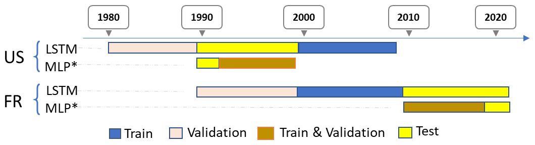
Figure 1 Train-test-validation split for both CAMELS-US and CAMELS-FR datasets. The test set (yellow), training set (blue), validation set (salmon), and combined training&validation set (marron) are indicated; the latter corresponds to training performed using cross-validation. MLP^* denotes the orchestrator used for discharge assimilation. Note that the entire modeling process of the DA strategies is carried out exclusively on the test period of the initial LSTM (or the benchmark) models.

Newman et al. (2017)Kratzert et al. (2019)

Table 1 Used features from the two datasets.

2 Materials and methods

2.1 Dataset

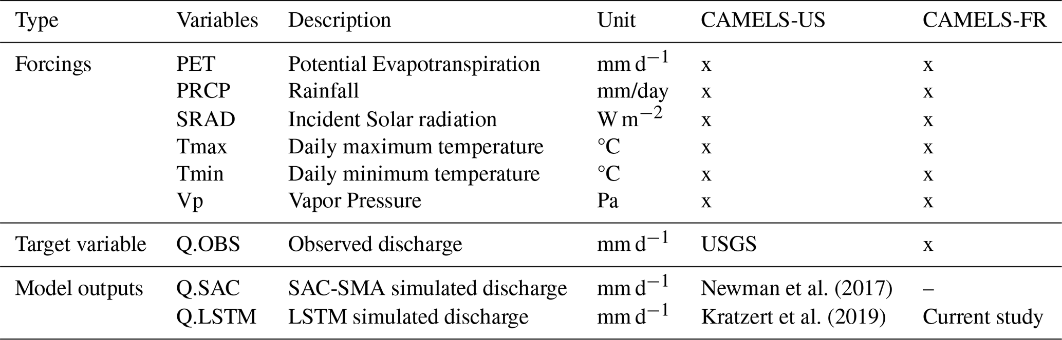
The CAMELS-US dataset (Addor et al., 2017) consists of basin-averaged hydrometeorological time series, catchment attributes, and daily streamflow observations from the United States Geological Survey (USGS) for 671 catchments across the Contiguous United States (CONUS). The meteorological forcings are available from Daymet, NLDAS, and Maurer sources. CAMELS-FR provides the same types of data for French catchments, of which a subset of 338 basins is considered in this study. As this study builds upon the benchmark works of Kratzert et al. (2019) and Newman et al. (2017), hereafter referred to as LSTM and SAC-SMA, it is limited to the same subset of 531 basins, the Maurer forcings, and the 1989–2008 period used in these previous works using the CAMELS-US dataset. For the CAMELS-FR dataset, an LSTM has been developed from scratch under the same approach as in Kratzert et al. (2019), then considered an equivalent benchmark. The usage of these variables is summarized in Table 1.

The added value of the proposed DA strategies is evaluated for two types of RR models: (a) the LSTM proposed in Kratzert et al. (2019), which was trained regionally and incorporates basin-specific static attributes, and (b) the conceptual global model SAC-SMA from Newman et al. (2017). As in Kratzert et al. (2019), the SAC-SMA model has been chosen as a reference to illustrate the performance of conceptual RR models, which remain widely used for operational discharge forecasting.

The train-test-validation split is illustrated in Fig. 1. It depicts how the data is divided for training, validation, and evaluation of the models. While the splitting of the initial models is mainly shown for reporting purposes, it provides a clear view of how the data are positioned for the tested DA strategies.

2.2 Discharge assimilation procedures

As outlined in Fig. 2 and described in Eqs. (1) to (5), three discharge assimilation procedures are tested, integrating either recent discharge measurements or simulations from the two RR models and using MLP as the orchestrator.

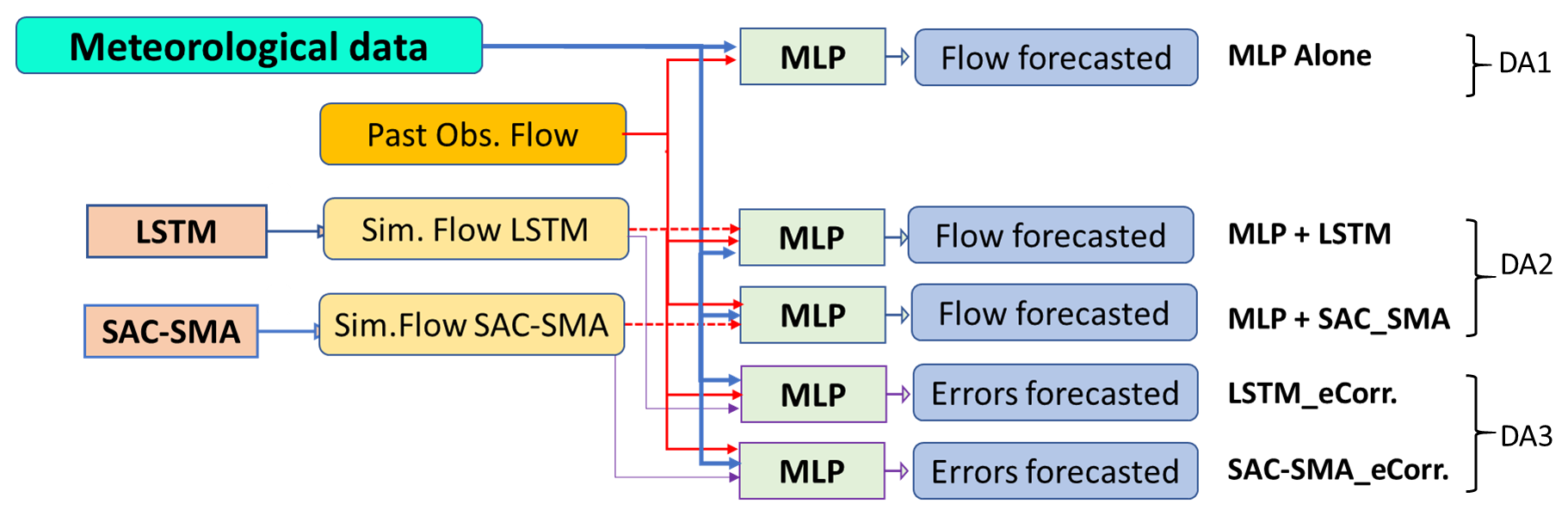
Figure 2 Discharge assimilation set-up: DA1, MLP Alone; DA2,MLP fed with RR model forecasts (MLP + LSTM or MLP + SAC − SMA); DA3, Post-treatment of RR forecasting errors noted as LSTM_eCorr and SAC-SMA_eCorr.

1. DA-1: direct forecast of discharges ${\widehat{Q}}_{t+hp}$ over the forecast horizon hp with an MLP, fed with the past observed discharges Q^o, observed meteorological variables X^o, as well as meteorological forecasts $\widehat{X}$ (see Eq. 1).

   $$\begin{array}{}\text{(1)}& {\widehat{Q}}_{t+hp}=f\left(Q_{t-p:t}^{\mathrm{o}},{\widehat{X}}_{t-n:t+hp},X_{t-n:t}^{\mathrm{o}}\right)\end{array}$$

2. DA-2: the same approach as in DA-1 but with the forecasts of the RR model Q^s (either SAC-SMA or LSTM) as additional input variables (see Eq. 2).

   $$\begin{array}{}\text{(2)}& {\widehat{Q}}_{t+hp}=f\left(Q_{t-p:t+hp}^{\mathrm{s}},Q_{t-p:t}^{\mathrm{o}},{\widehat{X}}_{t-n:t+hp},X_{t:t-n}^{\mathrm{o}}\right)\end{array}$$

3. DA-3: post-processing of the prediction errors of the RR model ε_t (again SAC-SMA or LSTM). In this strategy, the orchestrator is used to forecast the errors (${\widehat{\mathit{\epsilon }}}_{t+hp}$) of the RR model over the horizon hp and the prediction errors are then added to the forecasts of the RR model. The assimilation procedure then proceeds in three steps (see Eqs. 3, 4, and 5).

   $$\begin{array}{}\text{(3)}& {\displaystyle }& {\displaystyle }{\mathit{\epsilon }}_t=Q_t^{\mathrm{o}}-Q_t^{\mathrm{s}}\text{(4)}& {\displaystyle }& {\displaystyle }{\widehat{\mathit{\epsilon }}}_{t+hp}=f\left({\mathit{\epsilon }}_{t-p:t},Q_{t-p:t}^{\mathrm{o}},{\widehat{X}}_{t-n:t+hp},X_{t-n:t}^{\mathrm{o}}\right)\text{(5)}& {\displaystyle }& {\displaystyle }{\widehat{Q}}_{t+hp}=Q_{t+hp}^{\mathrm{s}}+{\widehat{\mathit{\epsilon }}}_{t+hp}\end{array}$$

In the previous equations, n and p are the sequence lengths for the forcing and the assimilated discharge. These values will be fixed based on the mean response time of the basins using a RR cross-correlation analysis; see Fig. 5. As suggested in Saint Fleur et al. (2020), to prevent the models from relying disproportionately on assimilated discharge rather than forcing, we imposed n≥p.

In summary, seven (7) different model configurations are compared: the five (5) DA procedures (unfolded from DA1, DA2, DA3) presented in this section, plus the two (2) direct forecasts from both pre-trained models, SAC-SMA and LSTM, which serve as benchmarks to evaluate the efficiency of the tested DA strategies. The direct forecasts from the benchmark models were assumed to be unchanged for the tested lead time; therefore, no further training was necessary.

In all the considered DA strategies and for each basin, the MLPs were trained (i.e., calibrated) 20 times, accounting for the random initialization (seeds) of their parameter values, leading to 20 different possible trained models. Likewise, 8 seeds have been considered for the LSTM and 10 for the SAC-SMA model. This aims to account for the uncertainties and variability induced by model initialization during training. The DA strategies are trained based on the series of mean simulated values of both benchmark models (SAC-SMA and LSTM). The predictions thus consist of an ensemble of 20 runs for the DA strategies and 8 and 10 runs for the LSTM and SAC-SMA benchmark forecasts without assimilation, respectively. The performances of the ensemble simulations (dispersed by random initialization) are analyzed based on their mean values in the first part of this paper (Sect. 3.1).

2.3 Forecasting setup and forecast products

2.3.1 Forecasting setup

In this study, the explored lead times range from 1 to 7 d. As illustrated in Eqs. (1), (2), and (5), the input feature selection for forecasting models incorporating discharge assimilation may be affected by the lead time (hp). In most feedforward architectures, a separate model is calibrated for each lead time. The alternative which consists of calibrating a single model across the entire range of lead times, either jointly or recursively, is generally inefficient, as it substantially amplifies the forecast uncertainty (Chevillon, 2007; Teräsvirta et al., 2010; Liu and Wang, 2024). This behavior has also been observed in the present study (results not presented herein). It is also worth noting that single-step models may not guaranty continuity of the outputs through successive lead times.

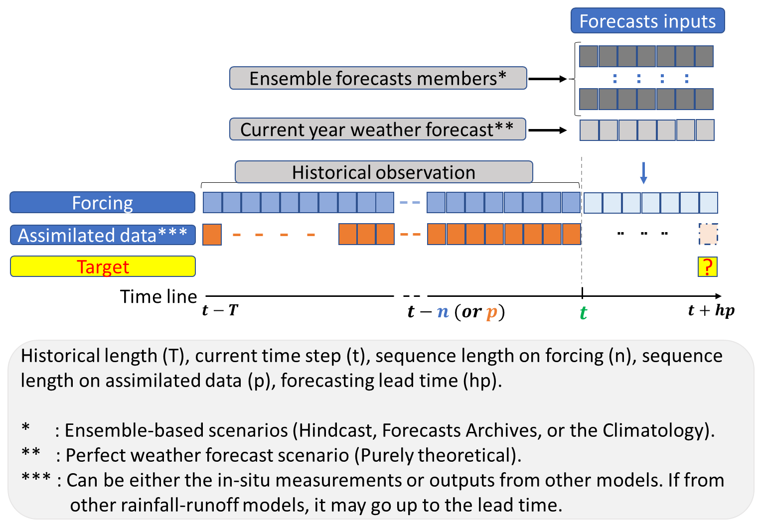
The forecasting framework is summarized in Fig. 3, which illustrates how past observations, assimilated discharge, and forecasted forcing data are integrated. The implementation in DA1 and DA2 procedures is straightforward for both the perfect and ensemble forecast strategies. However, for DA3 under the ensemble scenario, the corrected quantity corresponds to the forecast member ${\widehat{Q}}_{t+hp}^i$ for which the forecasted error ${\widehat{\mathit{\epsilon }}}_{t+hp}^i$ (in Eq. 4) is issued, where i indicates the forecast member.

Figure 3 Forecasting assumptions setup.

All the proposed DA strategies are trained using the perfect weather forecast configuration and then evaluated under both the perfect and the ensemble-based forecast conditions. The ensemble forecast evaluation is conducted using three sources of meteorological forcing: (1) a no-skill ensemble generated from past observations using a date-to-date sampling strategy, referred to as “Climatology”; (2) hindcast (reforecast) products; and (3) real-time forecast archives provided by the European Centre for Medium-Range Weather Forecasts (ECMWF). Hindcasts correspond to retrospective forecasts produced for past dates to establish a stable statistical reference for ensemble analysis, whereas real-time forecasts are operational predictions issued daily for current and future conditions. Their preparation for this paper is described in Sect. 2.3.2.

2.3.2 Hindcasts, forecast archives and the climatology approach

The operational evaluation is implemented using the sub-seasonal to seasonal (S2S) dataset (Vitart et al., 2017), developed through a joint initiative project of the World Weather Research Programme (WWRP) and the World Climate Research Programme (WCRP). At the time of writing this paper, the S2S database is hosted at ECMWF as an extension of the TIGGE archive. Overall, two forecast products are used: hindcast and real-time forecast archives. Since we evaluated the benchmark models (LSTM and SACSMA) over the 1989–1991 period, only hindcast-based evaluation is implemented on the CAMELS-US dataset because real-time archives are not provided for that period. Consequently, the hindcast product used is from the Bureau of Meteorology (BoM) database (Hudson et al., 2020). Nevertheless, to complement this analysis, the ensemble evaluation has been extended to the french basins using the CAMELS-FR dataset (Delaigue et al., 2025). This extension was specifically implemented on the two main DA approaches tested (LSTM and DA1), using both hindcast and forecast archives for the recent period of 2018–2021. On the ECMWF data portal (https://apps.ecmwf.int/datasets/data/s2s-realtime-instantaneous-accum-ecmf/levtype=sfc/type=cf/, last access: 10 February 2026), BoM and ECMWF forecasts are provided as separate products, allowing the use of both hindcast products and real-time forecast archives.

For the present analysis, the perturbed forecast from the BoM dataset was retrieved for up to 7 d of lead time, with all its 32 members. The same method was applied to gather the ECMWF forecast archives (50 members) and hindcast (10 members) products. It is worth noting that these open data are available mostly for 6 to 8 d a month.

We also implement the “Climatology” approach as a baseline, which represents the simplest alternative to archived weather forecasts. It is constructed by resampling historical meteorological observations. Although more sophisticated sampling strategies could be implemented, for example, by selecting periods of similar hydrological conditions (Hidalgo and Jougla, 2018), the present study adopts a simple date-to-date sampling strategy. For a current date (t₀) within the evaluation period (1989–1991 for CAMELS-US or 2018–2021 for CAMELS-FR), the sequence spanning the lead time ($t_{\mathrm{0}}:t_{\mathrm{0}}+h_p$) is defined. The same calendar sequence (day and month) is then extracted for each complete year in the remaining period (1991–2008 or 1989–2017), generating 18 ensemble members for the CAMELS-US cases and 29 members for the CAMELS-FR. This approach constitutes a typical no-skill or poor-man's ensemble, as its construction does not explicitly account for the predictability of non-periodic variables such as rainfall data. Nevertheless, it is conceptually similar to the Ensemble Prediction (ESP) framework introduced by Day (1985) and widely used in previous studies (Hidalgo and Jougla, 2018; Crochemore et al., 2017).

At the other end of the evaluation spectrum, the “Perfect forecast” configuration is also implemented. In this case, the forecasted meteorological variables are assumed to be equal to the actual observed values at the corresponding future lead time in the evaluation year. This configuration is particularly useful for estimating the theoretical upper bound of the performance of the models. Overall, four forecast configurations are considered in this study: Perfect Mode, Climatology Mode, Hindcast Mode, and Real-time Forecast Mode based on meteorological forecast archives.

2.4 Evaluation metrics

Numerous metrics are proposed in the literature to evaluate the skills of hydrometeorological forecasting models (Murphy, 1993; Seillier-Moiseiwitsch and Dawid, 1993; Bradley and Schwartz, 2011; Lai et al., 2011; Harold et al., 2015; Petropoulos et al., 2022): evaluating the efficiency for deterministic and ensemble predictions, as well as reliability and resolution for ensemble predictions (Bradley and Schwartz, 2011; Slater et al., 2019). The selected evaluation metrics are presented below.

2.4.1 Forecasting efficiency

The efficiency is a measure of the proximity between the observed values Q_t and the predicted values ${\widehat{Q}}_t$. The commonly used metrics for deterministic forecasts are based on the sum of squared errors: Nash–Sutcliffe Efficiency (NSE), Eq. (6) (Nash and Sutcliffe, 1970), the Kling–Gupta Efficiency (KGE) (Gupta et al., 2009), and the Persistency Criterion (PERS), Eq. (7) (Kitanidis and Bras, 1980; Corradini et al., 1986; Anctil et al., 2004).

$$\begin{array}{}\text{(6)}& {\displaystyle }& {\displaystyle }\mathrm{NSE}=\mathrm{1}-{\displaystyle \frac{\sum _{t=\mathrm{1}}^T{\left(Q_t-{\widehat{Q}}_t\right)}^{\mathrm{2}}}{\sum _{t=\mathrm{1}}^T{\left(Q_t-\stackrel{\mathrm{‾}}{Q}\right)}^{\mathrm{2}}}}\text{(7)}& {\displaystyle }& {\displaystyle }\mathrm{PERS}=\mathrm{1}-{\displaystyle \frac{\sum _{t=hp}^T{\left(Q_t-{\widehat{Q}}_t\right)}^{\mathrm{2}}}{\sum _{t=hp}^T{\left(Q_t-Q_{t-hp}\right)}^{\mathrm{2}}}}\end{array}$$

NSE and PERS are scores that measure the proportion of the sum of square errors of an unskilled model explained by the calibrated (or trained) forecasting model. The unskilled benchmark model for NSE is the trivial mean model (${\widehat{Q}}_t=\stackrel{\mathrm{‾}}{Q}$), and for PERS the persistent model (${\widehat{Q}}_{t+hp}=Q_t$). Both criteria range from 1 (perfect model) to −∞. A negative value indicates that the model produces higher errors and, consequently, performs worse than the unskilled benchmark models. It should be noted that it is more difficult to achieve a positive PERS than a positive NSE, particularly at short lead times.

For ensemble forecasts, the Continuous Ranked Probability Score (CRPS), Eq. (8) (Hersbach, 2000; Matheson and Winkler, 1976), is commonly used.

$$\begin{array}{}\text{(8)}& \begin{array}{rl}\mathrm{CRPS}& ={\displaystyle \frac{\mathrm{1}}{T}}\sum _{t=\mathrm{1}}^T{\mathrm{CRPS}}_t\mathrm{with}{\mathrm{CRPS}}_t\\ & =\underset{-\mathrm{\infty }}{\overset{\mathrm{\infty }}{\int }}{\left[F_t\left(y\right)-{\mathbf{1}}_{\left\{y\ge Q_t\right\}}\right]}^{\mathrm{2}}\mathrm{d}y\end{array}\end{array}$$

where, for time step t, F_t is the cumulative distribution of the ensemble forecasts, Q_t is the observed value, ${\widehat{Q}}_t$ is the predicted value, $\stackrel{\mathrm{‾}}{Q}$ is the time average of the observed values, and ${\mathbf{1}}_{\mathit{\{}y\ge Q_t\mathit{\}}}$ is the Heaviside-step function for a binary 0|1 outcome. The CRPS ranges from 0 (perfect models) to +∞ (low-quality models). Note that the CRPS is the mean absolute error of the model in the case of a deterministic forecast (i.e. ensemble constituted of a unique member).

2.4.2 Forecasting reliability

An ensemble forecast is considered reliable (or statistically consistent) when the ensemble spread adequately reflects forecast uncertainty, such that the observations are statistically indistinguishable from the ensemble members (Talagrand et al., 1997; Whitaker and Loughe, 1998; Hamill, 2001; Buizza et al., 2005). The resulting distribution of the ranks of a sufficient number of observations, as proposed in Hamill (2001) and Talagrand et al. (1997), provides a visual verification of the reliability of the ensemble forecasts. The lack of reliability may take different forms: (i) a tendency to overestimate (resp. underestimate), leading to an over-representation of the lower (resp. higher) ranks in the rank diagram; (ii) under- or over-dispersions of the ensembles, resulting in a U-shape or dome shape of the rank diagrams. Figure 4 shows the rank diagrams of the evaluation period (1989–1991) throughout the remaining period (1991–2008), for the daily rainfall and PET data.

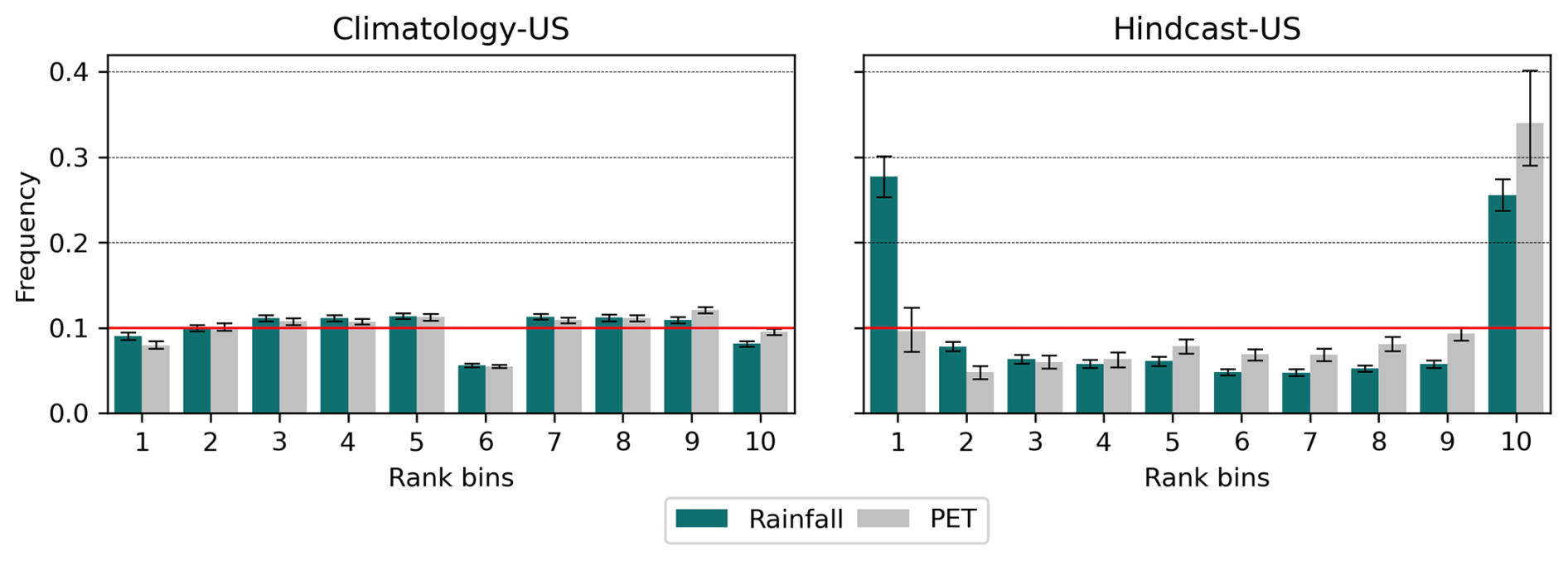
Figure 4 Rank diagrams for daily precipitation and PET for the Climatology-based ensemble (left panel) and Hindcast products (right panel) over the CAMELS-US basins for 3 d lead time. The plots correspond to the evaluation of the test-period (1989–1991) within the remaining 1991–2008 period. The error bars represent variability across the 56 basins considered, and the red line denotes the expected uniform distribution. For ease comparison, the ensembles have been condensed into 10 classes from 17 and 32 members, respectively.

The rank diagram of the climatological ensemble does not reveal any major deviations from the expected uniform distribution (Fig. 4), suggesting the absence of obvious biases in this ensemble. However, the uniformity is not observed in the hindcast product, which exhibits noticeable underdispersion that may be reflected in the forecasted discharges. This underdispersion, which varies within the lead times (see Appendix A8), remains an open question in the present study. Nonetheless, as mentioned by Hamill (2001), rank diagrams may mask certain defaults in ensemble forecasts; therefore, they will be complemented here by spread-skill ratio (SSR) analysis.

$$\begin{array}{}\text{(9)}& \begin{array}{rl}& \mathrm{SSR}={\displaystyle \frac{\sqrt{\frac{\mathrm{1}}{T}\sum _{t=\mathrm{1}}^T{\mathit{\sigma }}_t^{\mathrm{2}}}}{\sqrt{\frac{\mathrm{1}}{T}\sum _{t=\mathrm{1}}^T{\left({\stackrel{\mathrm{‾}}{x}}_t-y_t\right)}^{\mathrm{2}}}}}\mathrm{with}\\ & {\mathit{\sigma }}_t^{\mathrm{2}}={\displaystyle \frac{\mathrm{1}}{N-\mathrm{1}}}\sum _{i=\mathrm{1}}^N{\left(x_{t,i}-{\stackrel{\mathrm{‾}}{x}}_t\right)}^{\mathrm{2}}\end{array}\end{array}$$

where x and y denote forecast and observed values; N and i, the full-set and individual forecast members; T and t, the evaluation period length and time step. The spread-skill ratio (Eq. 9) is a widely used metric to evaluate the reliability of ensemble forecasts. It compares the ensemble spread (the forecast uncertainty) with the actual forecast error (skill) of the ensemble mean. As formalized by Whitaker and Loughe (1998), it is typically calculated as the ratio of the square root of the mean of the ensemble variance (spread) to the root mean squared error (RMSE) of the ensemble mean. Values close to one indicate a well-calibrated ensemble, while values below (above) one reveal under- (over-) dispersion.

2.4.3 Forecasting resolution

In ensemble forecast verification, resolution refers to the ability of a model to discriminate between events and non-events: i.e., the exceedance or non-exceedance of a given threshold discharge for hydrological predictions. Commonly used metrics for such evaluation include the Brier score (Brier, 1950) and the AUC score (Area Under the Curve) estimated based on a ROC (Receiver Operating Characteristic) curve.

• Brier score (BS)

$$\begin{array}{}\text{(10)}& \mathrm{BS}={\displaystyle \frac{\mathrm{1}}{N}}\sum _{i=\mathrm{1}}^N{\left(f_i-o_i\right)}^{\mathrm{2}}\end{array}$$

N is the number of time steps, f_i is the forecast probability of the event according to the ensemble, and o_i is the observed boolean outcome (1 if the event occurs and 0 otherwise).

The Brier score values range from 0 (perfect) to 1 and are equal to 0.25 for a random detection model (i.e., the no-skill model).

• ROC curves and AUC

To elaborate on the ROC curve; given a selected target discharge threshold, each rank of the ensemble is selected in turn as the forecast value for event detection. The True positive rate (TPR: proportion of observed events predicted as events) and the False positive rate (FPR: proportion of non-events predicted as events) are computed for each ensemble rank over the evaluation period. The ROC curve relates TPR and FPR. The AUC is the estimated area under the ROC curve. It takes its value between 1 (perfect model, TPR = 1 and FPR = 0 for all ranks) and 0. The ROC curve of a random detection model corresponds to the diagonal (i.e., TPR = FPR = proportion of predicted events). The AUC value of this random detection model is equal to 0.5.

The forecast resolution may depend on the chosen discharge threshold. To evaluate the ensemble forecasts, several threshold values are tested based on the quantile of the observed discharge series. The considered quantile probabilities are x of 0.01, 0.05, 0.10, 0.25, 0.50, 0.75, 0.90, 0.95, and 0.99. For a given discharge threshold Qx, an event is recorded whenever discharge values cross this threshold. For thresholds below the median (x≤0.5), events correspond to low-flow conditions, whereas high-flow (flood) conditions correspond to thresholds above the median (x>0.5). Exceedance is defined based on crossings from above (recession curve) or below (rising curve) the threshold, respectively.

2.5 Experimental settings

2.5.1 Input sequence size and lead time selection strategy

The sizes of the input sequences of the MLPs have been set based on cross-correlation diagrams; see Fig. 5 for the CAMELS-US dataset and Appendix A1 for the CAMELS-FR dataset. The median cross-correlation coefficients were considered in the 531 basins. Following Mangin (1984), a limit value has been chosen for the autocorrelation coefficient for discharges of 0.2 to fix the length p of the input sequence for the assimilated discharges. The sequence size (n) of the forcing has been set to 30 d as an arbitrary value along the flattened portion of the RR cross-correlogram.

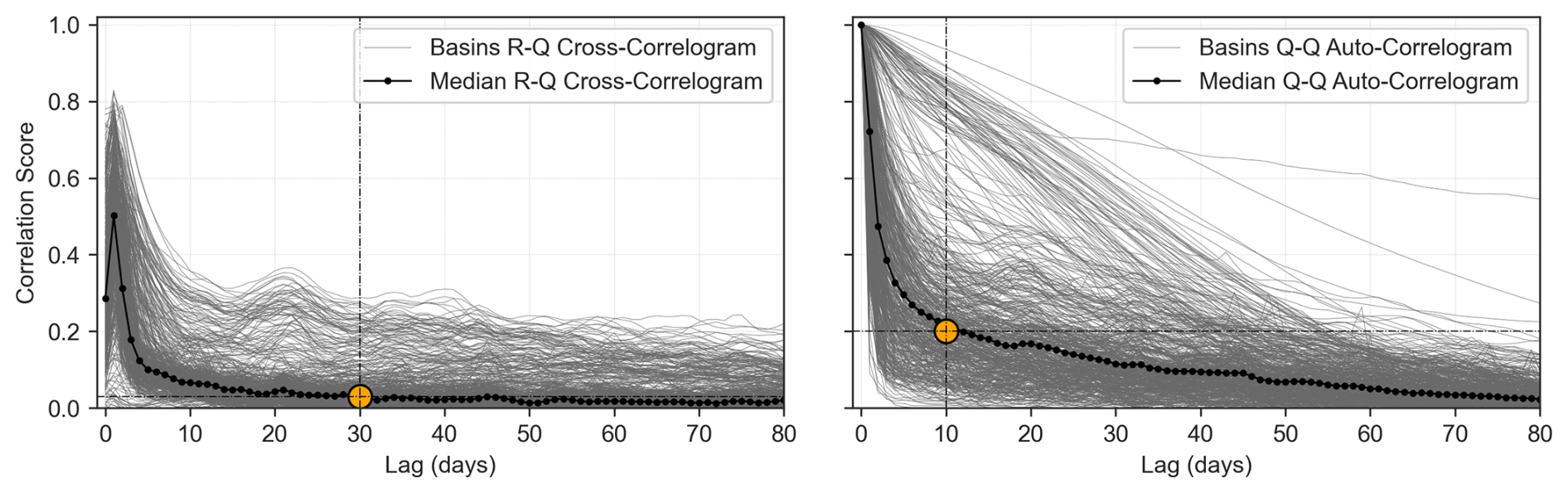
Figure 5 Rainfall–Discharge cross- and auto-correlation on the CAMELS-US dataset; see Appendix A1 for the CAMELS-FR case. The chosen sizes (n and p) of the input sequences are marked with the dashed lines and an orange-colored dot.

The correlation coefficients between observed discharges and daily rainfall amounts are highest for lag times between 1 and 3 d, suggesting that the basins of the CAMELS-US sample have, on average, short response times, typically of less than 3 d. This ensures that the evaluated 1 to 7 d lead times cover both short- and mid-range forecast horizons. According to the response times of the basins, it is anticipated that short-term predictions 1 d ahead will be partly controlled by past observed rainfalls, whereas mid-term 3 to 7 d forecasts will be mostly determined by predicted rainfalls.

2.5.2 Basin sub-sampling for the climatological ensemble runs

The evaluation of the ensemble-based forecast may be numerically demanding: 7 lead times, 7 model configurations, 20 randomly initialized models, 10 to 50 forecast members, and numerous trials for model hyperparameter searching and training. To keep reasonable computation times, the ensemble-based evaluations were conducted on a subset of 56 basins from the initial set of 531 basins. This subset of basins was selected uniformly according to their NSE rank from Kratzert et al. (2019), covering the same range of basins as the initial sample of 531 basins (Fig. 6). For the CAMELS-FR basins, the selection was based on the completeness of the discharge time series, with total missing data not exceeding 90 d, while ensuring that all regions (basins coded from A to Y) are represented. The lists of selected basins are provided within the code availability.

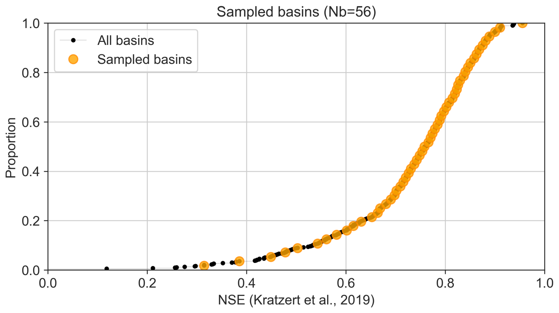
Figure 6 Cumulative distribution of the NSE scores of the 531 US-basins from the regional LSTM of Kratzert et al. (2019) and the selected subset of 56 basins.

2.5.3 Softwares and hyperparameter settings

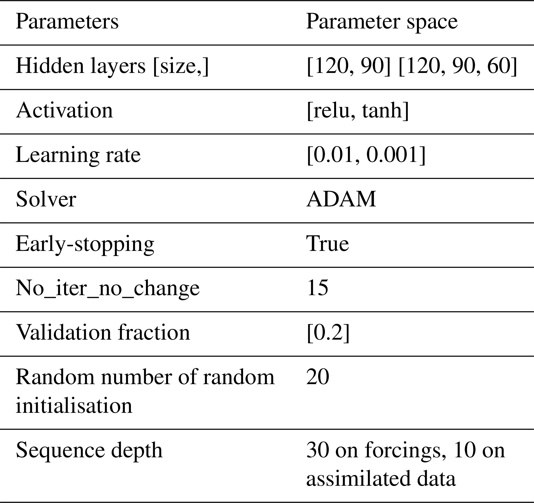
For the orchestrator (MLP) configurations, the hyper-parameters listed in Table 2 were optimized using exhaustive grid search and cross-validation with respect to the used datasets. The hyperparameter subset was derived from a larger space using 20 randomly selected basins, retaining the most frequent configurations. The hidden sizes ranged from a single layer of 30 neurons to four layers with multiples of 30 neurons. Five levels of learning rates (10⁻¹ to 10⁻⁵) were primarily tested, and two have been retained based on their occurrences as the best values.

Table 2 Model hyper-parameter setup.

The experiments developed in this study are essentially based on open-source software and the Python 3.9 programming language (van Rossum, 1995). Our modeling framework is based on the Scikit-Learn library (Pedregosa et al., 2012). Data analysis, processing, and visualization are performed mainly using Pandas (McKinney, 2010), Numpy (van der Walt et al., 2011), Seaborn (Waskom, 2021), Matplotlib (Hunter, 2007), and Xskillscore (Bell et al., 2021). The model development was carried out using Jupyter Notebook (Kluyver et al., 2016), Anaconda (Anon, 2020), and PyCharm (JetBrains, 2024).

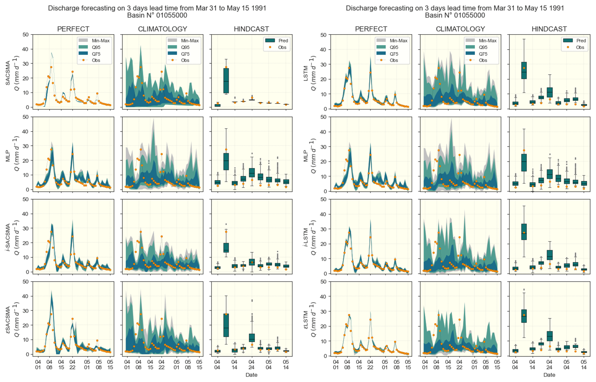
Figure 7 Examples of hydrographs on basin 01055000 of the CAMELS-US dataset for a 3 d lead time rainfall–runoff forecasting. SAC-SMA (left panels) and LSTM (right panels) cases are shown separately; rows indicates (benchmark models, DA1, DA2, DA3), and columns points to the meteorological forecasting approaches (Perfect, Climatology and Hindcast). Since hindcast products are available only 6 times a month, their outputs are discontinued and shown through box-plots for easier display. Color ranges are used to highlight ensemble quantile ranges Q₇₅ = [0.125, 0.875], Q₉₅ = [0.025, 0.975] and [Min, Max] values, while the observed discharge values are marked with orange-dots.

3 Results on the CAMELS-US dataset

The performance of the three discharge assimilation (DA) approaches is evaluated against the benchmark models across the considered forecast scenarios. This comparison emphasizes the differences in model behavior between an idealized setting (perfect forecast scenario) and several ensemble-based forecasts. The variability of the scores across the basins is illustrated using boxplots and error bars. To introduce the results, an example of hydrographs (observed and forecasted) is presented in Fig. 7. This example corresponds to basin No. 01055000 from the CAMELS-US dataset over the period from 31 March to 15 May 1991, and includes the three tested forecasting approaches (Perfect, Climatology, and Hindcast) along with both benchmark models (LSTM and SACSMA). All presented results concern the test set.

Figure 7 shows what each of the forecast results looks like. For illustration purposes, we selected a case in which both the benchmark models and the meteorological hindcast provide accurate results. The performance metrics and scores of the different approaches for the various lead times, evaluated in the full set of 531 CAMELS-US basins, are presented and discussed in the following sections.

Nearing et al. (2022)

Table 3 NSE and improvements at a 1 d lead time across tested discharge assimilation approaches and benchmark models from several studies.

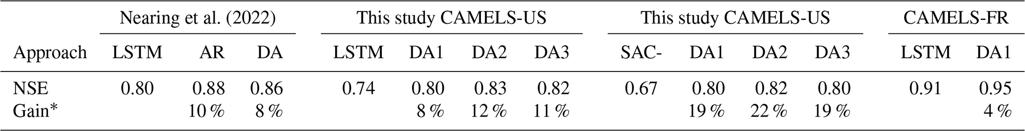
^* Gains are estimated relative to the benchmark model NSE. In Nearing et al. (2022), AR and DA refer to the methods called auto-regressive and discharge assimilation respectively. SAC- refers to SAC-SMA model.

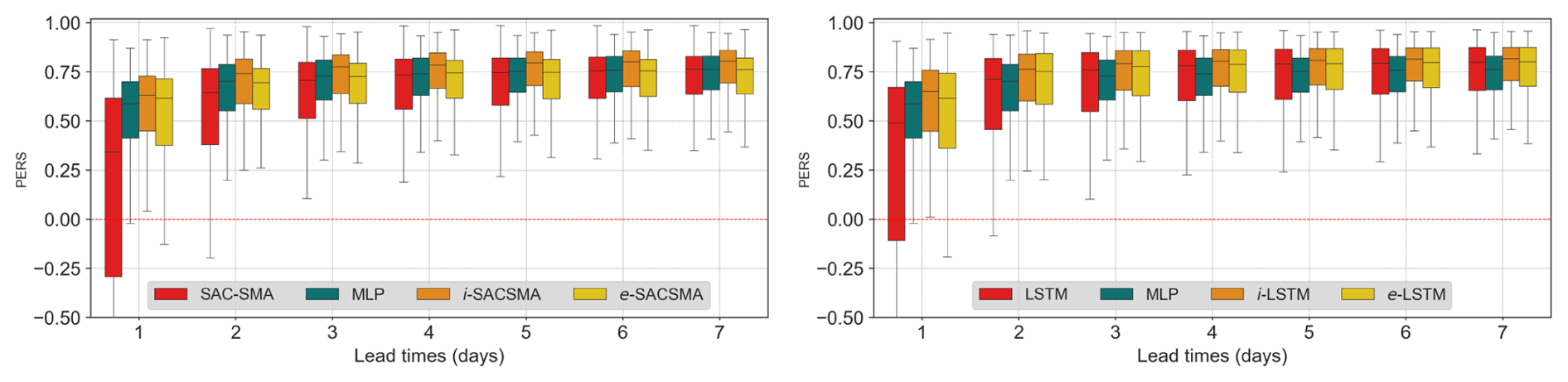
Figure 8 Box-plots of the persistence (PERS) scores. The figures are ordered with SACSMA-cases first, followed by LSTM-cases. Lead times (1–7 d) are shown on x axis, while scores are displayed on the y axis. Color-codes distinguish the approaches: benchmark models (red), DA1 or MLP (green), DA2 (orange) and DA3 (gold). DA1 is replicated in both benchmark cases. In the legend, i-LSTM stands for DA2 or MLP-informed by LSTM, e-LSTM stands for DA3 or error post-processing approach on the LSTM case.

3.1 Performances of the DA approaches based on perfect meteorological forecasts

3.1.1 Forecasting efficiency

As an introduction, Table 3 displays an overview of the NSE values and gains of the discharge assimilation methods tested in this study for the 1 d lead time forecast, compared to the results published in Nearing et al. (2022), which tested discharge assimilation using an LSTM on the same CAMELS-US dataset. Note that the test period differs between the study of Nearing et al. (2022) (1989–1999) and the present study (1989–1991). Table 3 also includes the results obtained on the CAMELS-FR dataset, which are presented in more detail in Sect. 4. It shows that NSE scores are highly dependent on the datasets and that the relative gains from discharge assimilation methods tend to be greater when the benchmark models have lower NSE values.

Overall, the improvements achieved by the DA strategies developed here are globally consistent with those reported in Nearing et al. (2022). NSE gains range from 8 % to 12 % for the LSTM model and reach up to 22 % for the conceptual SAC-SMA model. As explained in Sect. 2, the remaining analysis is based on the persistence analysis (Fig. 8), which provides more contrasted results than the NSE score.

As expected, the PERS scores (Fig. 8) are lower at short lead times. This is a common outcome in persistence analysis, as models generally struggle to outperform the persistent model at very short horizons: the smaller the discharge variations, the more difficult they are to predict. Furthermore, in agreement with previous studies, performances are significantly higher for the LSTM-cases than for the SAC-SMA and this trend persists even when DA procedures are implemented.

The DA1 method appears to be more effective than the SAC-SMA benchmark in all the lead times tested. However, it only clearly outperforms the benchmark LSTM model in the 1 d lead time when the initial PERS scores of the LSTM are modest: the median PERS values lower than 0.5 and the PERS values lower than 0 for 20 % of the basins.

For further clarity, Fig. 9 summarizes the gain in PERS scores achieved by the different DA procedures relative to their corresponding benchmark models. Almost without surprise, these gains are highly dependent on the initial PERS value of the benchmark model. Three classes of initial benchmark PERS values are considered in the figure to illustrate this dependency: (−∞, 0], [0, 0.5], and [0.5, 1]. The two other DA strategies, DA2 and DA3, both based on the benchmark models (i.e., MLP-informed and error post-processing), prove to be effective, as they consistently improve the performance of the benchmark forecasting models on which they are based. DA2 outperforms DA1, while the DA3 approach generally enhances performance or, at least, preserves performance when it is already high.

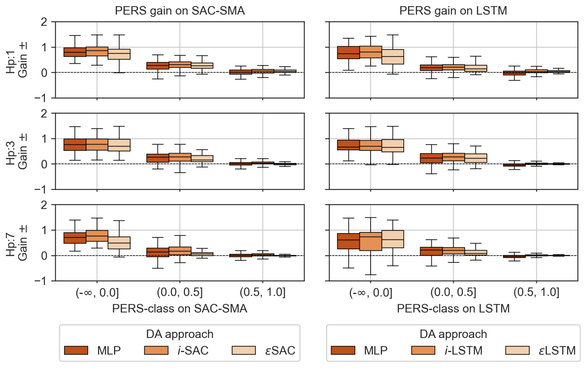
Figure 9 Gain on Persistence. Where, Gain = DA − Benchmark. For lighter nomenclature, the following names have been respectively used: MLP simple (MLP), MLP Informed by BM (i-SAC or i-LSTM), benchmarks error post-processed (ϵSAC or ϵLSTM).

The two Figs. 8 and 9 show that the gains are larger for shorter lead times, more pronounced for SAC-SMA than for LSTM due to the overall lower scores of the SAC-SMA model, and lower for basins where the initial model already performs well. In general, the ranking of the approaches tested is strongly dependent on the initial skills of the benchmark models. DA2 appears to be the most effective approach overall, followed by DA3 (Fig. 8).

These results demonstrate the effectiveness of the proposed DA strategies in improving forecast performance under a perfect meteorological forecast scenario. Gains are particularly significant for the 1 d lead times. However, the added value of the proposed DA decreases rapidly with increasing lead times (Fig. 9). This decline can be explained by both the increase in the PERS benchmark models with lead time and the overall short response times of the basins in the CAMELS-US dataset, which typically range from one to a few days. This is depicted by the cross-correlation analysis (Fig. 5), which explains the reduced influence of past discharges on future trajectories for horizons exceeding these response times.

The next step consists of assessing whether these conclusions remain valid when taking into account uncertainties in meteorological forecasts, a situation that corresponds to the operational implementation of rainfall–runoff forecasting models. To streamline the discussion while considering the superiority of the LSTM model compared to Sac-SMA and other possible conceptual rainfall–runoff models, only the LSTM cases are considered in the remainder of the present manuscript.

3.2 Performances of the DA approaches under ensemble-based forecast scenarios

As a reminder, for the examples based on the CAMELS-US dataset, the ensemble forecast scenario is implemented using the historical meteorological records (i.e., Climatology) and the BoM hindcast data. According to the adopted sampling strategy, the Climatology-ensemble consists of 18 members (1991–2008), whereas the hindcast ensemble consists of 32 members, as provided by the data source. The hindcast product is discontinuous, as only 6 predictions are issued within a month. To account for model uncertainties, these ensembles are further expanded through random model initialization: 8 realizations for the LSTM and 20 for the DA approaches. To limit computational costs, the evaluation is conducted in a representative subset of 56 basins, selected to cover the range of LSTM NSE (test) values observed in the 531 basins of the CAMELS-US dataset, as shown in Fig. 6. Three key properties of the forecast ensembles are evaluated here: (1) their efficiency based on the CRPS score, (2) their reliability based on rank diagrams complemented with spread/skill ratios (SSR), and (3) their resolution using Brier and AUC scores.

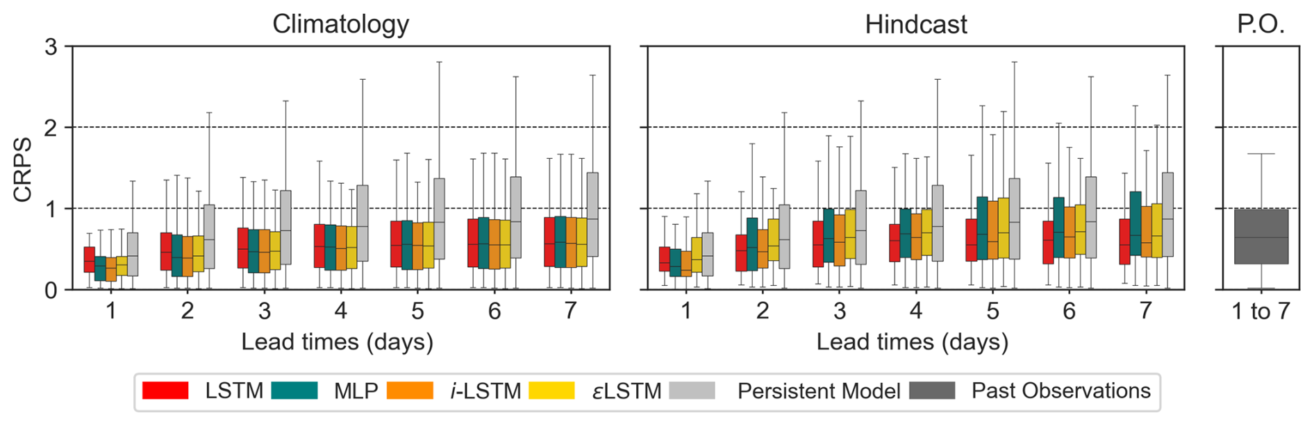
Figure 10 Box-plots of the CRPS scores for the 56 tested basins for the 1989–1991 test period. Lead times of 1 to 7 d are shown in x axis, while sores are displayed in y axis where 0 denotes perfect forecasts. Colors indicated the LSTM benchmark (red), DA1 (green), DA2 (dark-orange), DA3 (gold), Persistent Model (gray) and Past-Observed discharge (dark gray).

3.2.1 Forecast efficiency

Figure 10 presents the CRPS values for both forecast scenarios based on climatological ensembles and forecasts in all approaches and lead times tested for DA. Two baseline models are included in the analysis: the persistent model (forecast equal to the last observed discharge) and the past-observed (P.O) discharge model, which consists of discharge observations from previous years on the considered date. Since the Persistent-Model produces a single deterministic prediction, its CRPS is reduced to the mean absolute error (MAE). In contrast, the P.O model comprises 18 members and is therefore treated like all other ensemble forecasts.

According to Fig. 10, all tested models appear more efficient than the persistent baseline model for all lead times, even when accounting for uncertainties in the ensemble forecasts. The performance gap between these models and the persistent model becomes larger as the forecast lead time increases.

In the climatology-based scenario (left-most), the models consistently outperform the baseline observed in the past (P.O.), signifying that all tested models and approaches remain informative even at the larger lead times. However, this pattern is not consistently observed in the hindcast-based scenario for lead times exceeding 3 d. The observed biases in the BoM hindcast products for the period 1989–1991, and for the estimated basin average daily PET and rainfall (Fig. 4), clearly limit the efficiency of ensemble forecasts based on these hindcasts for the CAMELS-US basins. A detailed analysis of the structure of these biases, along with the development of an appropriate bias correction method (Zalachori et al., 2012; Yang et al., 2020) would be essential to fully exploit the potential of these hindcasts. However, this likely complex task was beyond the scope of the present study.

Finally, the observed trends in Fig. 10 (climatology) are consistent with those observed using the PERS criterion under the perfect meteorological forecast scenario (Fig. 8) with some nuances. The DA approaches, including DA1 (simple MLP), remain effective, as they globally improve the performance of the LSTM model or, at least, do not degrade it for any of the tested lead times. Their added values are also more pronounced at shorter lead times.

3.2.2 Forecast reliability

Figure 11 shows the rank diagrams for both the climatology- and hindcast-based scenarios with the CAMELS-US dataset. The ensemble members have been grouped into 10 classes for all models to facilitate comparisons. The figure is organized vertically, and the results of the LSTM benchmark model are shown in the first row, followed by the three tested DA approaches.

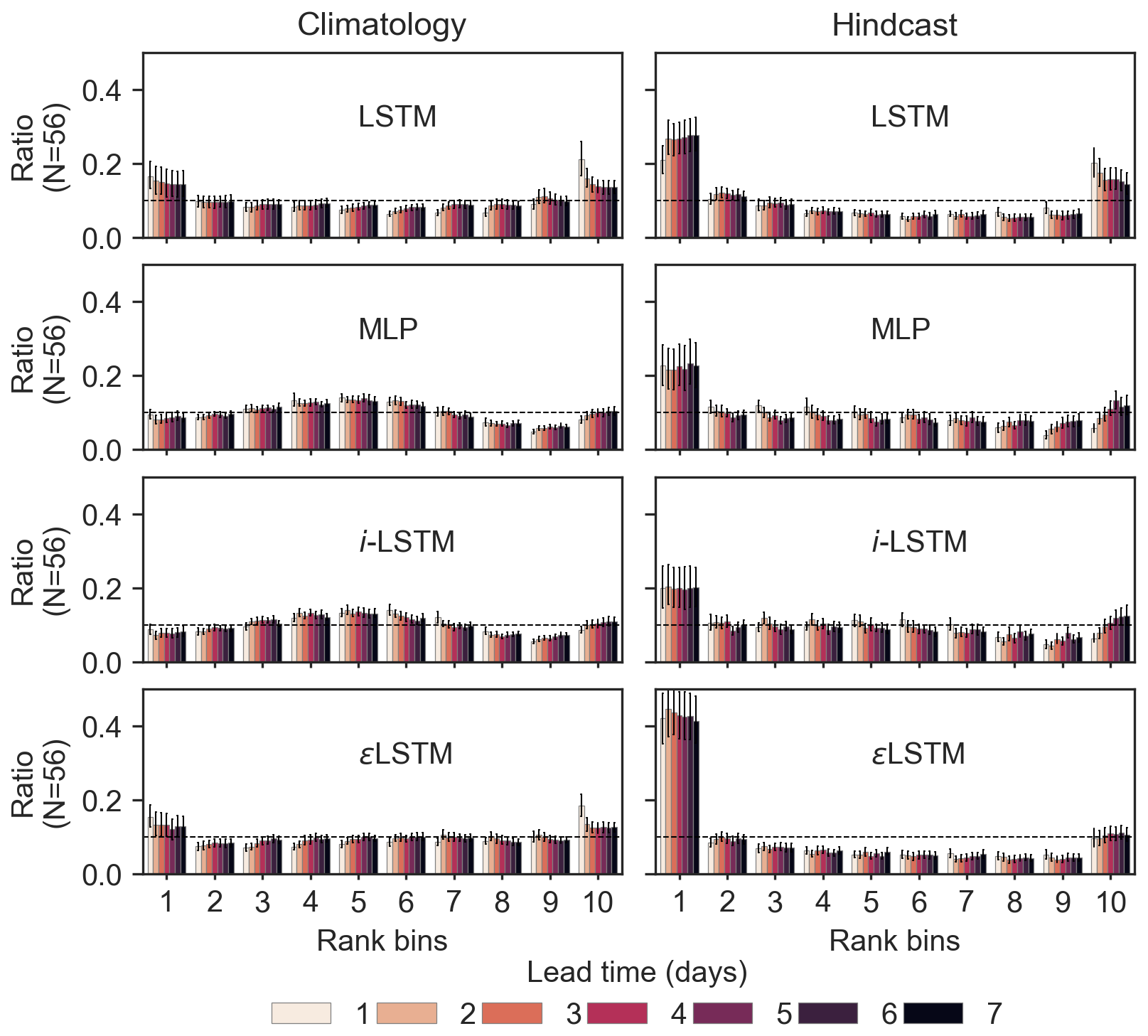
Figure 11 Rank diagrams for the LSTM-cases models and the DA strategies. x axis (10 rank classes), y axis (proportion of observed values in each class), median ratio and error-bars indicating the distributions for the 56 basins. Colors indicate the lead times.

Reliable forecasts are expected to yield uniformly distributed rank diagrams, indicating ensemble forecasts in which actual events are evenly distributed across all forecast member ranks. It should be noted first that the rank diagrams are similar across all lead times for a given model and meteorological ensemble product, and they differ between models, indicating that the rainfall–runoff forecasting model, including the discharge assimilation procedure, has an impact on the spread and possible biases of the forecast ensembles. The rank diagrams indicate that the hindcast biases (Appendix A6) propagate in all models and methods tested, providing an explanation for the lower observed CRPS values compared to the climatology-based scenario. The U-shape of the hindcast-based forecast rank diagram suggests that the forecast ensembles may be, on average, under-dispersed. This pattern is not evident when looking at model outputs (Fig. 7), but it seems to be confirmed by the spread-skill ratios, which are significantly lower for hindcast-based forecasts than those of the climatology-based forecasts (Fig. 12). A slight deviation from the uniform distribution also appears in the rank diagram of the LSTM climatology-based ensemble forecasts. The spread-skill ratios of the LSTM model appear similar to those of the DA1 (MLP), DA2, and DA3 approaches, suggesting that the possible biases in the ensembles generated by the rainfall–runoff model are more complex than simple systematic under-dispersion.

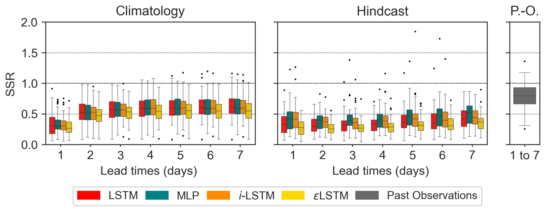
Figure 12 Box-plots of the spread-skill ratio for both climatology- (left panels) and hindcast-based (right panels) forecast scenario for the subset of 56 basins. LSTM-cases (LSTM, DA1, DA2 or i-LSTM, DA3 or e-LSTM) cases are shown including the Past-observed (P.O.) discharge model.

3.2.3 Forecast resolution

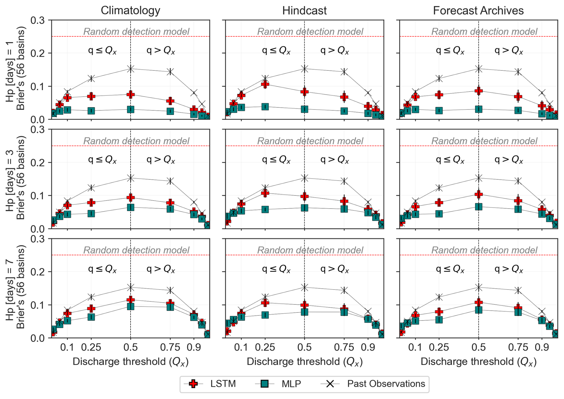
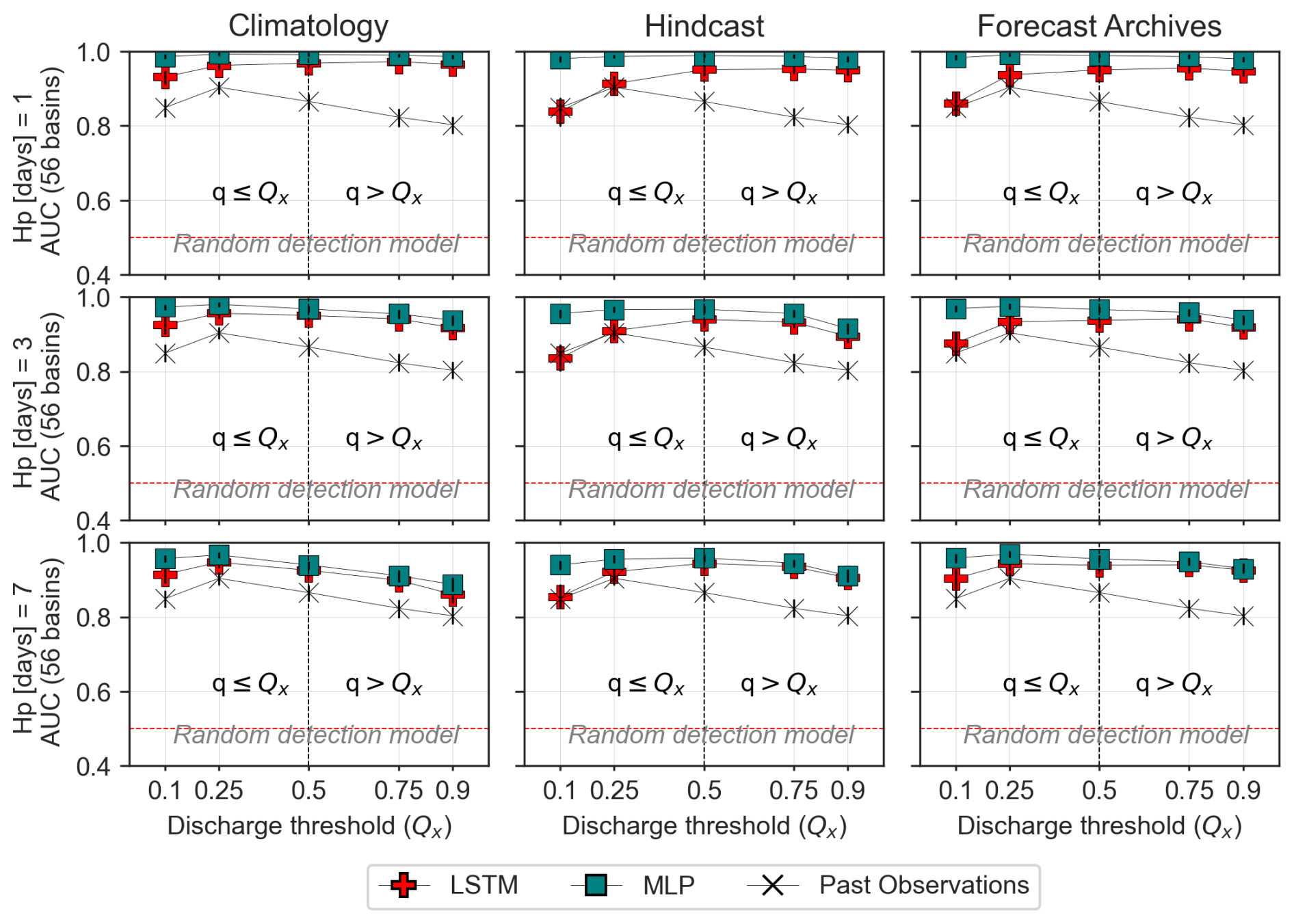
The Brier's and AUC scores evaluate the ability of an ensemble forecast to anticipate events and non-events; for instance, the exceedance or non-exceedance of a selected discharge threshold. Their values are presented in Fig. 13 and 14. As expected, the resolution of all forecasting approaches tested decreases with increasing lead times; i.e., the computed brier scores and AUC get closer to the values obtained based on past observations only for all thresholds as the lead time increases. The resolution analysis also confirms the poor skill of the ensemble forecasts based on the hindcast as used here, which is particularly noticeable in the Brier scores (Fig. 13).

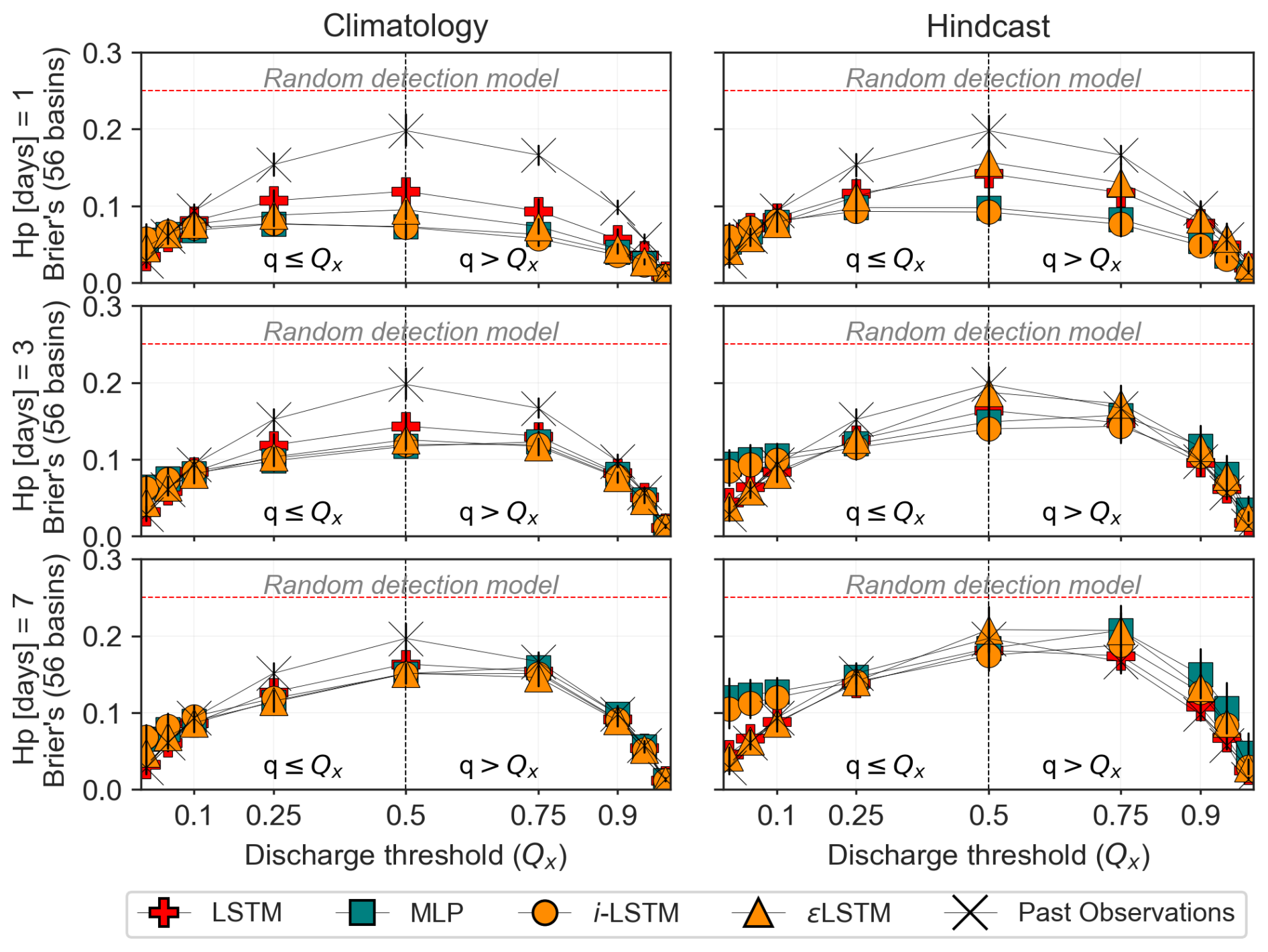
Figure 13 Brier's Scores for event detection based on thresholds using discharge quantile (Q_x) for both low flow (q≤Q_x) and high flow (q>Q_x) values. Median scores and error-bars are shown, indicating the dispersion across the subset of 56 test basins. Past-observed discharge is also evaluated as a poor man's discharge forecast and represented by the X symbols.

All the approaches tested outperform the random detection model (Brier = 0.25) and generally surpass the P.O model under climatology-based forecasts, with little to no improvement under the hindcast-based forecast. The earlier finding that climatology-based ensembles tend to outperform hindcast-based forecasts in terms of forecast resolution is also observed here.

The previous conclusions also hold for the model resolution: the proposed DA strategies prove effective. They either significantly improve the skill of the LSTM benchmark or, at least, do not degrade its initial performance.

This is particularly clear in the Brier scores (Fig. 13), especially for short lead times and intermediate discharge thresholds. The AUC graph shows less pronounced contrasts (Fig. 14). For a more in-depth comparison between methods, an example of the Roc curves obtained for the threshold quantile 0.95 is presented in Appendix B2. It illustrates the complexity of the comparison: the relative ranking of the models depends on the lead times, criteria, range of considered discharge values or thresholds, and also the target probability of detection in the ROC curve.

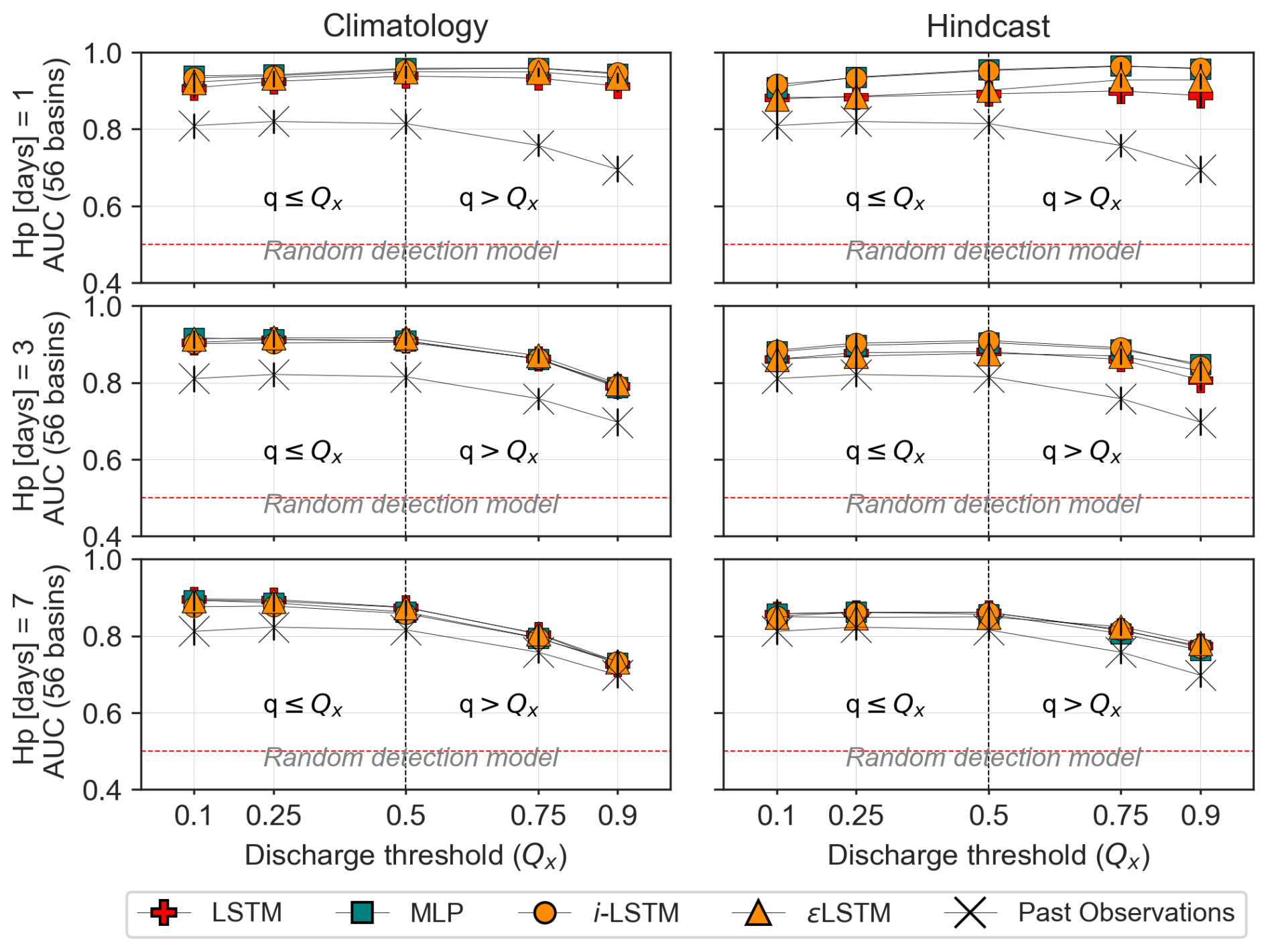
Figure 14 AUC scores for events based on flow quantile [0.1, 0.25, 0.5, 0.75, 0.9], with drought/flood detection shifting at quantile 0.5. These shown values correspond to the median AUC values across 56 basins. Climatology and Hindcast are shown in rows, lead times 1-3-7 d are presented in columns. Past-observed discharge is also evaluated as a poor man's discharge forecast and represented by the X symbols.

Two additional observations can be drawn from the AUC figure (Fig. 14), despite its limited contrast. First, the gap between AUC values based on past observed discharges and those of the tested forecasting approaches is particularly pronounced for high-threshold quantiles at a 1 d lead time. This suggests that the tested approaches are particularly well-suited to predicting the exceedance of high discharge values, which is consistent with the fact that the standard root mean square error criterion, known to place greater emphasis on large discharge values (Terven et al., 2025), has been used to train all models and methods.

More surprisingly, for large discharge thresholds at 3 and 7 d lead times, the AUC scores obtained with hindcast-based approaches exceed those associated with climatology-based forecasts. This indicates that, despite their apparently lower overall skill, the hindcast products used contain valuable information compared to climatology for predicting intense rainfall-triggered events.

These observations further illustrate how conclusions drawn from model comparisons depend on the target variable used to train the model, the range of values considered, and the evaluation metric used. At this stage of the analysis, the following partial conclusions can be drawn:

• The proposed discharge assimilation procedures, particularly DA2 and DA3, prove to be effective, as they either significantly improve or at least do not degrade the performance of the LSTM benchmark model across all considered lead times and evaluation criteria;

• Evaluating rainfall–runoff forecasts based on meteorological ensembles is a necessary complement to analyzes that are often conducted under the implicit assumption of perfect meteorological forecasts. In the present case, this approach reveals that the superiority of the LSTM and LSTM-based discharge assimilation methods over the proposed simpler MLP model, observed for lead times greater than two days, disappears once meteorological uncertainties are taken into account.

Nevertheless, the analysis is limited by the low skill of the available hindcast products for the selected test period (1989–1991) in the CAMELS-US dataset. It is therefore proposed in Sect. 4 to implement some of the tested approaches on a more recent dataset (CAMELS-FR), for which additional ensemble meteorological forecast products are available. The objective of this extension is twofold: (1) to assess the robustness and generality of the conclusions drawn from the CAMELS-US case study, and (2) to evaluate ensemble forecasting skill using more recent and probably higher-quality meteorological ensemble forecasts produced by the European Center for Medium-Range Weather Forecasts (ECMWF).

In line with the conclusions of this section, and for the sake of simplicity, the analysis in Sect. 4 is restricted to the benchmark LSTM model and the DA1 (MLP) strategy, evaluated under the same framework as previously. The analysis relies on hindcast products as well as forecast archives, providing an evaluation of the predictive skill of these two ensemble rainfall–runoff forecasting models, had they been implemented in the past.

4 Extension to the CAMELS-FR dataset

To ensure consistency with previous studies, such as Kratzert et al. (2019) for the CAMELS-US dataset and Hashemi et al. (2022) for French basins, Fig. 15 illustrates the position of the NSE values for the LSTM and DA1 approaches implemented in this extended analysis using the CAMELS-FR dataset (Delaigue et al., 2025). The results indicate that the trained LSTM achieves a high level of performance on the CAMELS-FR dataset, with median NSE values reaching 0.9.

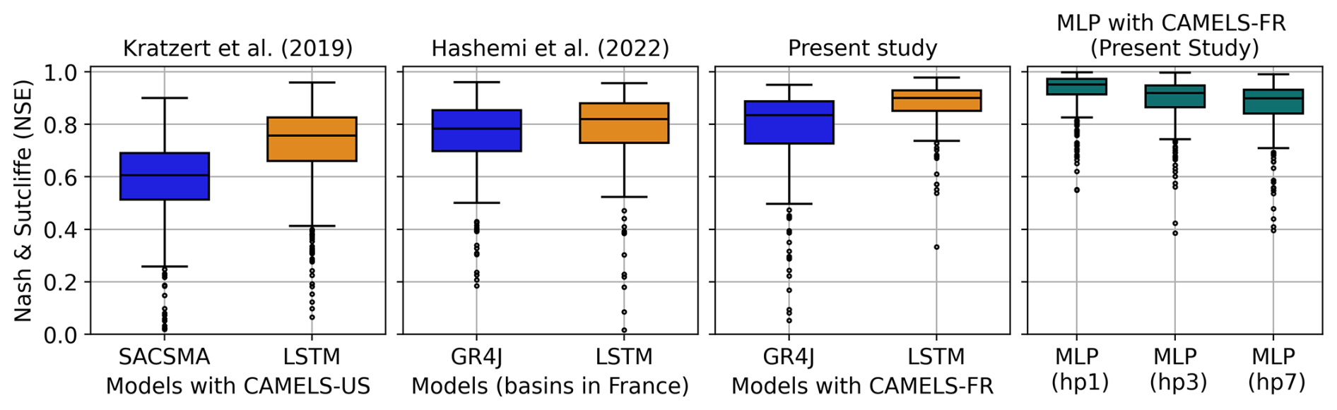
Figure 15 NSE scores comparison between LSTM and SACSMA for 531 US-basins with Kratzert et al. (2019), LSTM and GR4J (Perrin et al., 2003) on 365 French basins with Hashemi et al. (2022), and the ongoing LSTM vs GR4J and MLP (DA1) for 338 basins from the CAMELS-FR dataset.

Furthermore, consistent with the comparison presented in Sect. 3, the DA1 outperforms the LSTM at the 1 d lead time and exhibits NSE values comparable to those of the LSTM model at longer lead times. The NSE values obtained on the same datasets with the conceptual GR4J model (Perrin et al., 2003), a reference model in France, are also shown. These results confirm that AI-based rainfall–runoff forecasts outperform traditional conceptual rainfall–runoff models on the French dataset, although the performance gap is less pronounced than that reported in Kratzert et al. (2019) for US basins.

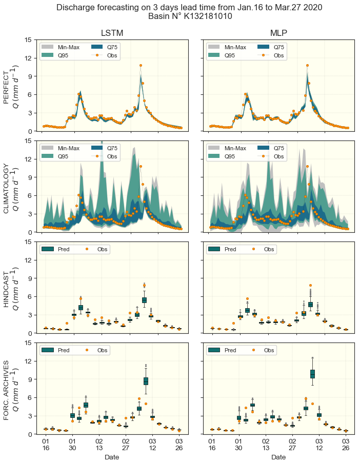
Figure 16 Example of 3 d lead time forecasted hydrograph for the basin K132181010 from 16 January to 27 March 2020. LSTM and DA1 are displayed in columns, while the 4 forecast approaches (Perfect, Climatology, Hindcast and Forecast Archives) are in rows. Given discontinuity in the two last forecast products, they are represented using box-plots.

It can also be observed in Fig. 15 that the NSE values increase from left to right. Since the LSTM architectures and implementation strategies are similar across the considered studies ¹, this increase may be partly explained by the improvement over time of the model training algorithms but is probably mainly attributable to the datasets; the recently published CAMELS-FR dataset consists of records from basins with limited anthropogenic influence and has undergone extensive quality control (Delaigue et al., 2025).

Figure 16 illustrates, using an example of hydrographs from the CAMELS-FR experiment, what the outcomes of the various approaches tested look like. The 3 d lead time forecast is presented here, while the corresponding 1 and 7 d lead times are provided in Appendix B5. Nevertheless, no general conclusion can be drawn from this isolated example regarding the relative performance of the various methods. Furthermore, direct pairwise comparisons between hindcast and forecast archives are not possible, as the dates for which the hindcast and forecast archives are available are not strictly aligned. The aggregated evaluation metrics are presented hereafter.

4.1 Model efficiency analysis

The PERS scores obtained by the LSTM and DA1 approaches for the CAMELS-FR (Appendix B6) exhibit trends similar to those observed in the CAMELS-US analysis; however, the median PERS of the MLP (DA1) method remains higher than that of LSTM up to the 5 d lead time. This can be partly explained by the difference in hydrological inertia of the basins between the two datasets, as shown in Appendix A1 and previously discussed by Pelletier and Andréassian (2024). In the same line of thought, the spread of PERS scores for the DA1 remains more limited than that of the LSTM model across all the tested lead times. While these differences may also partly originate from variations in dataset quality and initial model performance, they also reflect the contribution of the assimilated discharges, which certainly plays a key role.

4.2 Ensemble forecast analysis (efficiency, reliability and resolution)

In this subsection, the complete ensemble analysis is provided, using CRPS scores (Fig. 17) for the efficiency analysis, the Rank diagram (Fig. 18) for reliability, and Brier's scores (Fig. 19) for the resolution of the ensemble forecasts. The Spread-Skill ratio and the AUC scores are provided in Appendices B7 and B9, respectively.

Figure 17 CRPS scores for the LSTM and the DA1 (MLP) with the CAMELS-FR dataset.

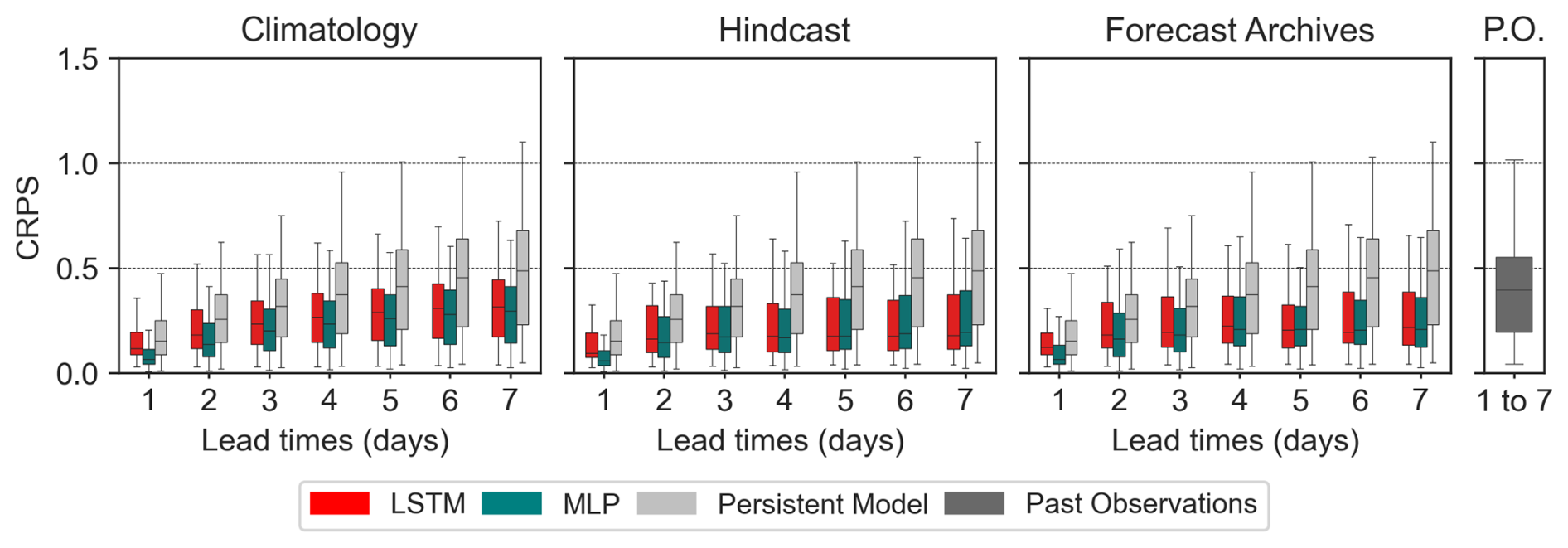
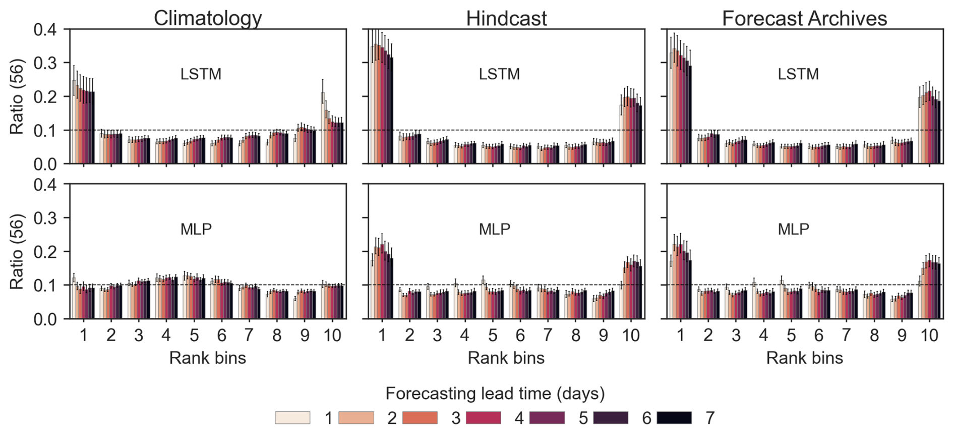
Figure 18 Rank diagrams for the benchmark models and the DA strategies. x axis (10 rank classes), y axis (proportion of observed values in each class), median ratio and error-bars indicating the maximum and minimum ratios for the 56 test basins. Colors indicate the lead times.

Figure 19 Brier's Scores for the LSTM and the DA1 (MLP) with the CAMELS-FR dataset.

As shown in Fig. 17, CRPS values are generally lower here than those reported previously, with most values falling below 0.5 across all forecasting approaches, including the Climatology-based method. All tested methods (LSTM and DA1) successfully outperform both the persistent model and the no-skill past observed (P.O) discharge ensembles.

Unlike in the CAMELS-US case, meteorological ensemble forecast products (hindcast and forecast archives) demonstrate better performance than the climatology-based ensemble, particularly for lead times exceeding 2 d. This is further supported by the CRPSS scores (Appendix B8), estimated using the climatology-based forecast as a reference, which indicate that both forecast products outperform this baseline.

Note that this result, counterbalancing the pessimistic conclusion drawn in Sect. 3 regarding meteorological hindcasts, is obtained despite the significant biases observed in both the hindcast and forecast products used in this French experiment (see Figs. A7 and A8).

Consistent with the persistence criterion, the CRPS values obtained with the DA1 (MLP) approach are, on average, lower (better) than those of the LSTM model across all meteorological ensembles and lead times, except for the hindcast at lead times exceeding 4 d.

The rank diagrams (Fig. 18) reveal biases affecting all forecast ensembles. With the exception of the climatology-based MLP forecasts, an excessively high proportion of observed discharges falls outside the [0.1, 0.9] quantile range of the forecast ensembles. This is partly explained by the biases in the hindcast products and the forecast archives (Fig. A7). However, as these proportions are higher for the LSTM model, it is likely that this model also introduces additional biases when combined with weather forecast ensembles.

This issue certainly deserves further investigation to support a more efficient operational implementation of LSTM-based rainfall–runoff forecasting models. Biases in forecast ensembles reduce the resolution of the forecasts, as the probability of exceedance is less accurately represented.

Consistent with the analysis in Sect. 3, all models and approaches outperform both the random detection and the past-observed discharge ensemble baselines. However, unlike in Sect. 3, this statement clearly holds across all meteorological ensembles, lead times, and evaluation metrics (Brier in Fig. 19 and AUC in Fig. B9).

The resolution of the DA1 (MLP) strategy appears higher than that of the LSTM across most tested configurations, with the exception of the Brier scores computed for the low discharge threshold at a 7 d lead time (Fig. 19). In this case, the CRPS of the LSTM models appears, on average, lower than that of the DA1, suggesting some consistency across metrics in capturing various properties of the forecasts.

Two specific patterns identified in the AUC analysis in Sect. 3 are also visible in Fig. B9. First, the gap between AUC values based on past-observed (P.O) discharges and those of the forecasting models is particularly pronounced for high-threshold quantiles at a 1 d lead time. Second, for large-discharge thresholds at a 7 d lead time, the AUC scores obtained with hindcast- and archive-based ensemble forecasts clearly exceed those of the climatology-based forecast. This confirms the ability of the weather forecast products to predict significant rainfall events up to one week in advance.

Overall, this extended analysis, which incorporates forecast archives, yields satisfactory results. It confirms the findings of Sect. 3 and reinforces the relevance of the forecasting and discharge assimilation (DA) approaches evaluated in this study. The main findings are as follows: (1) the gain of the DA1 strategy compared to the rainfall–runoff LSTM simulation model is consistently observed, although it is lower for the CAMELS-FR basins, partly due to the initial high performance of the LSTM; (2) the complementarity of the two forecast evaluation frameworks (deterministic vs. ensemble-based) further highlights the importance of ensemble-based evaluation in operational hydrometeorological forecasting. Ensemble-based forecasting also emphasizes the superiority of the DA1 approach over the rainfall–runoff LSTM across the tested lead times and evaluation metrics. Finally, this extended analysis suggests a higher quality of ensemble weather forecast products over the recent period (2018–2021) used to evaluate the DA approaches in the CAMELS-FR basins.

5 Conclusions

This work aimed to evaluate the added value of discharge assimilation (DA) procedures for rainfall–runoff forecasting, particularly in the context of AI-based operational hydrometeorological applications. Three DA strategies are compared against two benchmark models (LSTM and SAC-SMA) that do not incorporate DA. These DA strategies are evaluated under both a traditional perfect weather forecast (deterministic) framework and an ensemble-based forecast framework, using no-skill past observed forcing (climatology), hindcast products, and forecast archives. Additional emphasis is provided through comparisons with both a persistent model and past-observed (P.O) discharge ensembles. The experiments have been conducted on the widely used CAMELS-US dataset and extended to the recently published CAMELS-FR dataset.

While all tested approaches consistently outperform both the persistent model and the P.O baselines, the various DA procedures appear to be globally effective. They generally improve, or at least do not significantly degrade, the forecasting performance of the benchmark models on which they are based. Within the perfect meteorological forecast evaluation framework, DA approaches consistently improve the SAC-SMA forecasts, while improvements for the LSTM are mainly observed at short lead times and in basins where the benchmark LSTM model initially underperformed. These more limited gains further highlight the strong performance of the LSTM model in rainfall–runoff simulation and forecasting, as already demonstrated in numerous studies (Kratzert et al., 2019; Feng et al., 2020; Hashemi et al., 2022; Nearing et al., 2022; Yang et al., 2025). This behavior is consistently observed across both CAMELS-US and CAMELS-FR basins. Due to the higher hydrological inertia of the CAMELS-FR basins compared to those of the CAMELS-US, the added value of the tested DA strategies remains significant at longer forecasting lead times.

Several interesting insights emerge from the ensemble-based evaluation framework. The DA1 (MLP) approach, which incorporates past observed discharges, appears to outperform the LSTM model across all the tested lead times. This conclusion holds particularly for the assessment criteria characterizing the resolution of the forecasts (Brier's scores and AUC); i.e., the ability to detect in advance the exceedance of a discharge threshold. The LSTM model appears penalized by the limited reliability of its forecast ensembles (biases observed on the rank diagrams). This ensemble evaluation suggests that the performance of the LSTM forecasts could be improved in the future through the implementation of post-processing techniques such as ensemble bias correction.

The tested DA methods are implemented using a relatively simple MLP orchestrator, which already provides satisfactory results. Although this choice aligns with the objective of developing frugal AI solutions, there remains clear potential for improvement by exploring more advanced AI techniques and alternative data assimilation strategies, such as the Ensemble Kalman Filter (Clark et al., 2008) or an auto-regressive approach as in Nearing et al. (2022).

It is observed that model performances are globally higher for high observed discharge values than for low flows. This is likely related to the use of the mean squared error loss function during training (Terven et al., 2025). The investigation of alternative loss functions tailored to different flow levels, therefore, represents a promising direction for future research, particularly for the development of AI-based low-flow forecasting models. Moreover, as ensemble discharge forecasts are becoming an operational standard, it may be beneficial to train models directly using ensemble-based metrics, for example, by optimizing the Brier's score for event detection purposes.

Further work could also focus on a more thorough analysis of meteorological and hydrological ensemble spreads, as well as on the application of ensemble bias correction methods to improve the resolution of forecast products.

Appendix A: Data and specificity

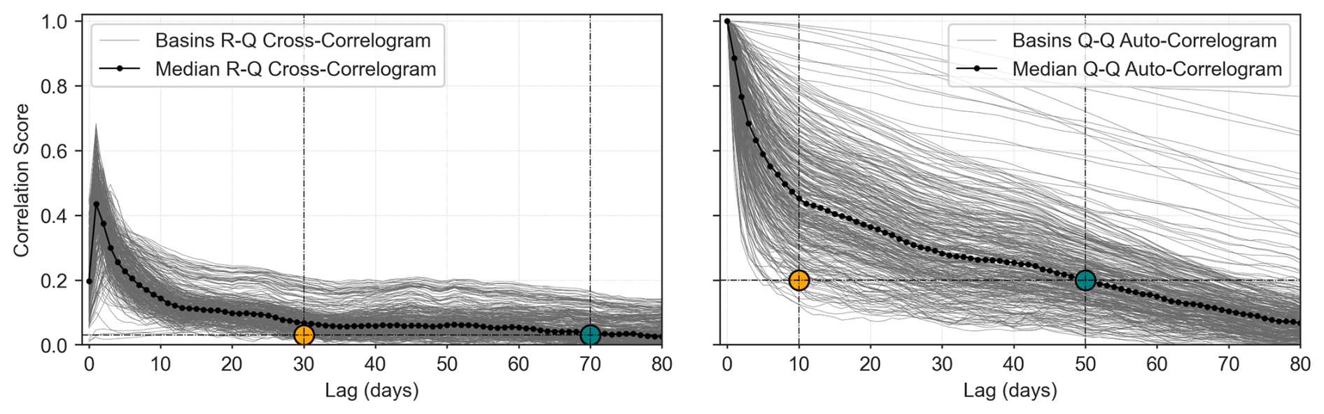
Figure A1 Cross- and auto-correlation analysis between the rainfall and the discharge for the CAMELS-FR dataset. Orange dots denote the position of the n and p used on the CAMELS-US dataset, whereas the teal one indicate the corresponding cross-correlation scores for the CAMELS-FR dataset. This means, following the same approach to setup the size of the input sequences, larger values would have been used on the CAMELS-FR cases.

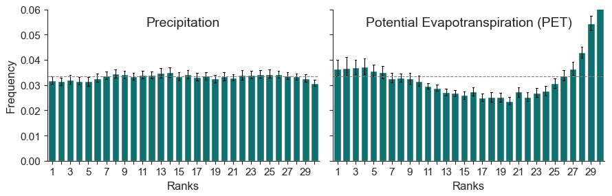
Figure A2 Rank diagrams for Rainfall and PET on CAMELS-FR dataset comparing the test period to the remaining historical observations.

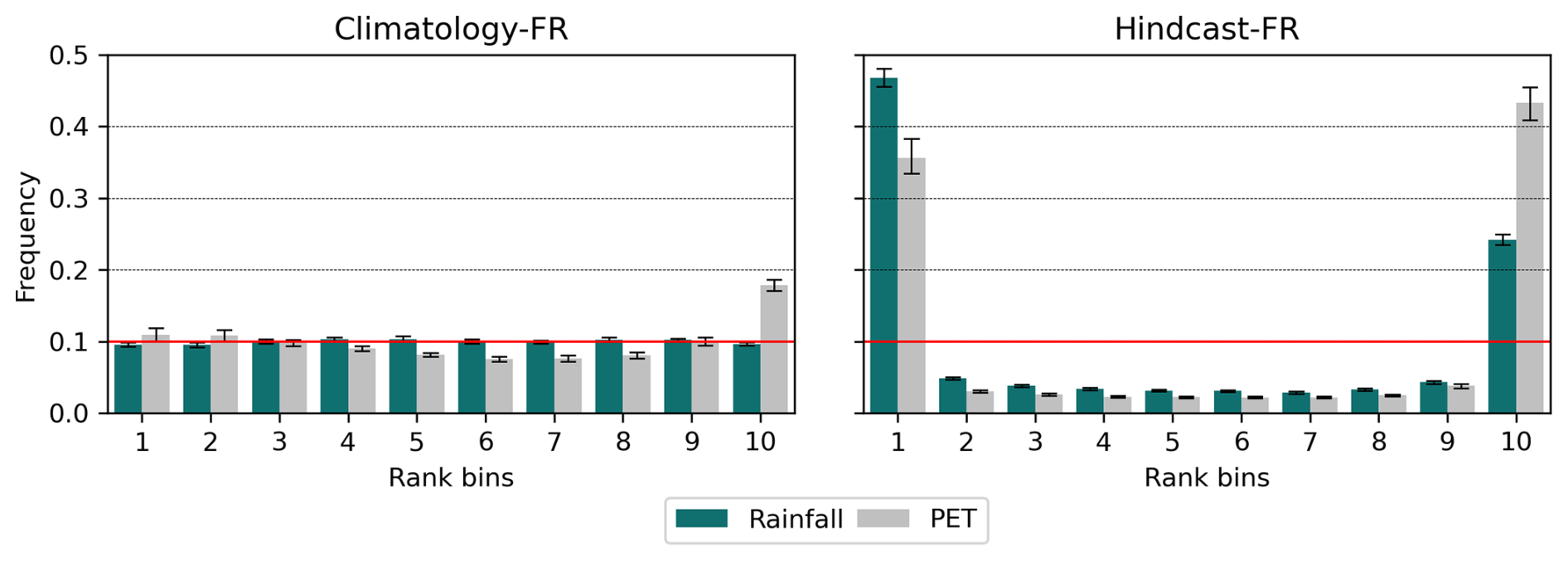
Figure A3 Rank diagrams for the daily precipitation and PET for the climatological ensembles (left panel) and Hindcast (right panel) products for the CAMELS-FR dataset. Plots correspond to 1989–2017 and evaluated for the test period 2017–2021. The error-bars represent variability for the 56 tested basins, the red line denotes the expected uniform distribution

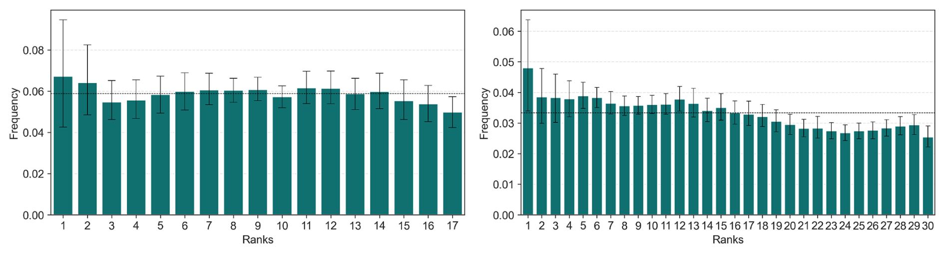
Figure A4 Rank diagrams of the test period against the remaining data for the discharge (discharge climatology) for CAMELS-US (left panel) and CAMELS-FR (right panel) datasets.

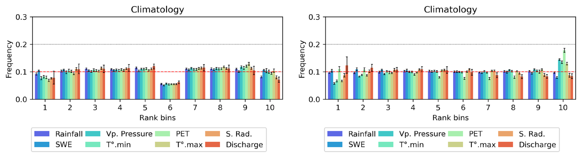
Figure A5 Dispersion analysis of the climatology for all the features in both CAMELS-US (left panel) and CAMELS-FR (right panel) datasets. For easier visualization, the 18 and 29 members the two datasets have been forced to be displayed on 10 classes per graphic.

Figure A6 Dispersion analysis of the forecast products on the CAMELS-US case.

Figure A7 Dispersion analysis of the forecast products on the CAMELS-FR case.

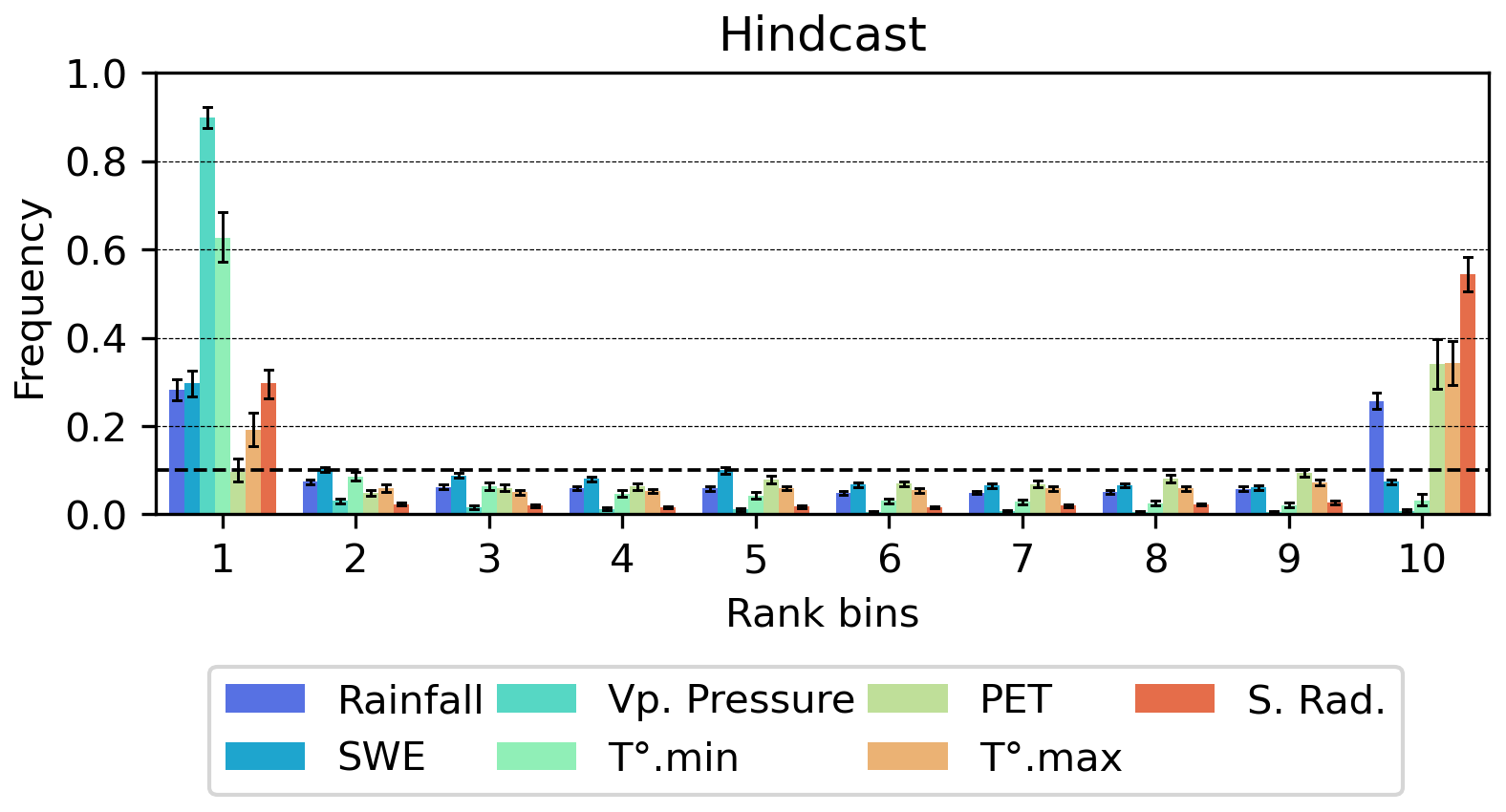
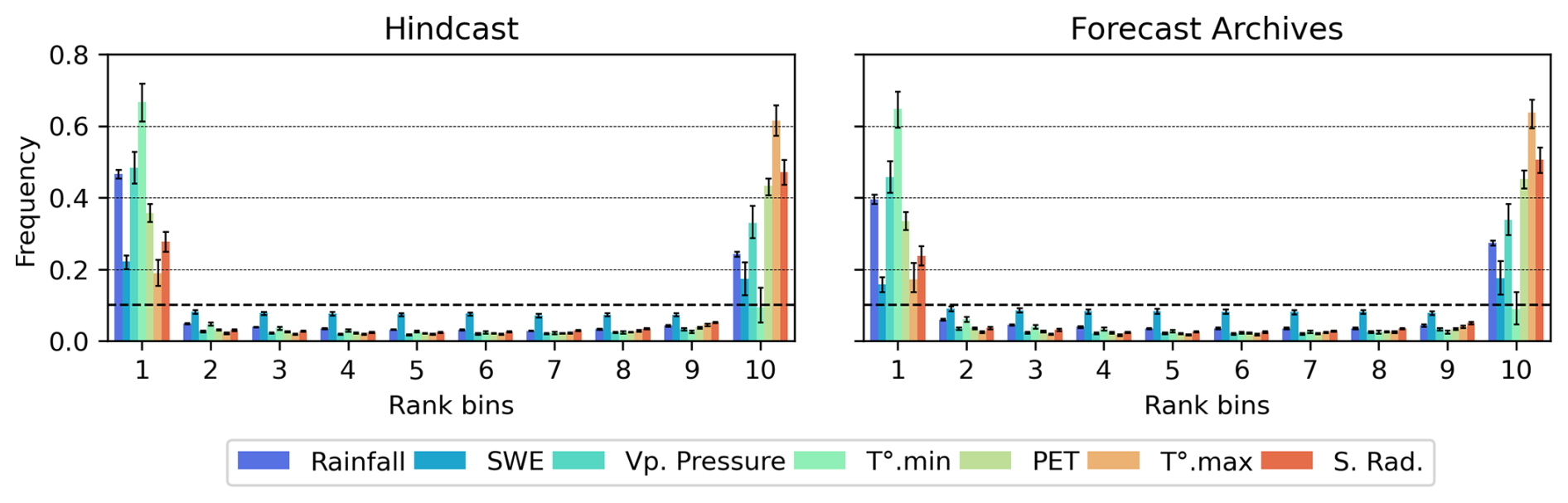
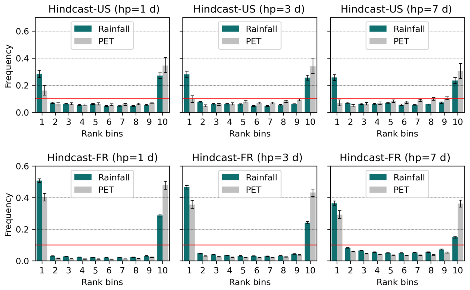
Figure A8 Rank diagrams for daily precipitation and PET for the Hindcast-based ensemble, for lead times 1, 3, and 7 d for both US-basins (top panels) and FR-basins (bottom panels). The plots correspond to the evaluation of the respective test-period within the respective forecast data. The error bars represent variability across the 56 basins considered, and the red line denotes the expected uniform distribution. For ease comparison, the ensembles have been condensed into 10 classes from 32 and 10 members, respectively. Under-dispersion trend of the hindcast products appears diminished within increasing lead times.

Appendix B: Hydrograms

Figure B2 provides an illustration of the ROC curves based on which the AUC values have been calculated, as well as the variability of the ROC curve shapes across the 56 test basins. One ROC curve and one AUC value are computed for each basin and each forecasting method tested.

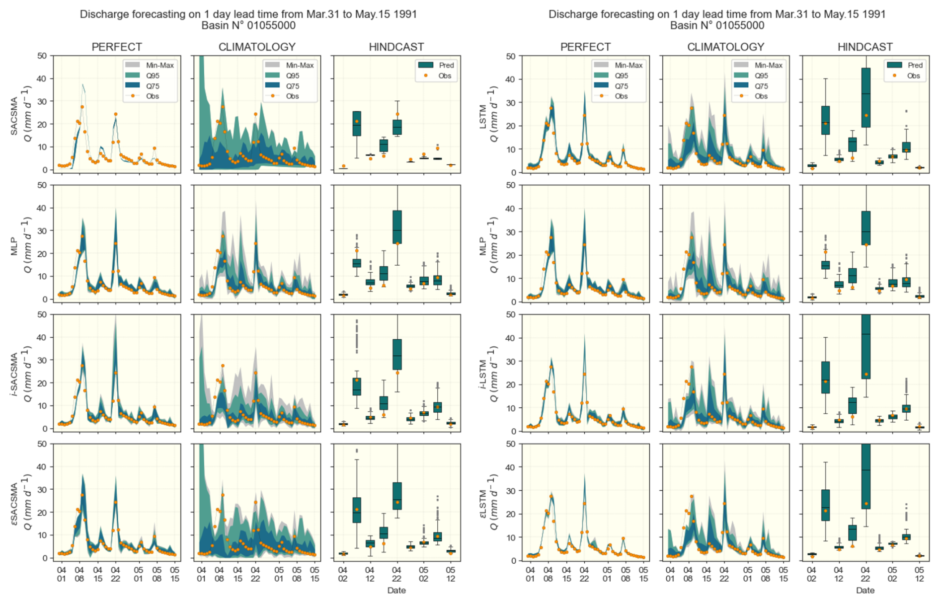
Figure B1 Example of hydrograph for 1 d lead times on the CAMELS-US dataset for both SACS-SMA (left panels) and LSTM (right panels) cases for basin No. 01055000.

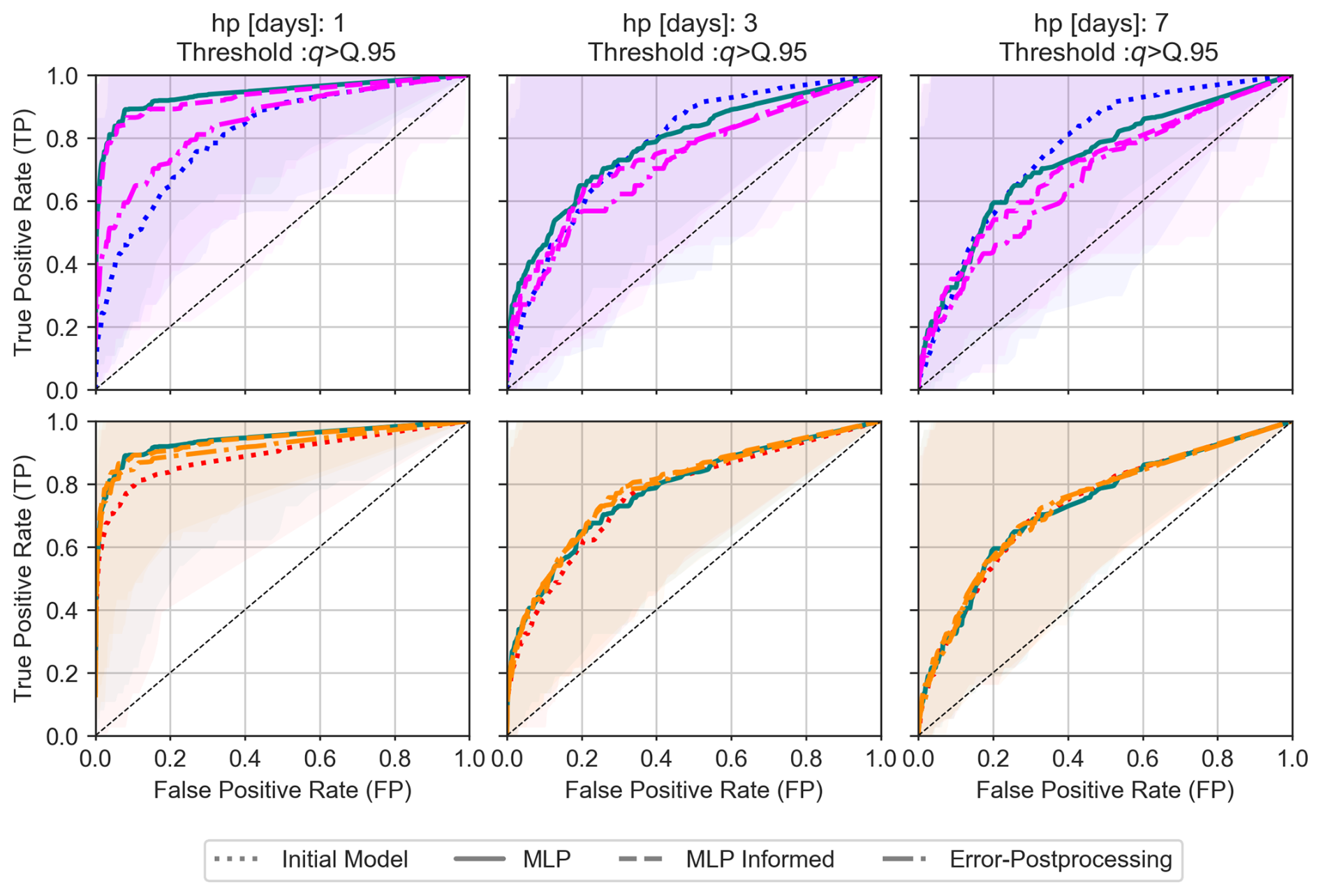
Figure B2 ROC curves for flood detection (q≥Q₉₅) for 1, 3 and 7 d lead times. Results are style-coded: MLP Simple (green solid, DA-1), MLP informed by benchmark (dashed, DA-2), Benchmark ePP (dot-dashed, DA-3), initial Benchmark (dotted). Benchmark cases are color-coded: SACSMA (blue to pink, first row), LSTM (red to orange, second row). Halos show the variability across the 56 basins around the median values.

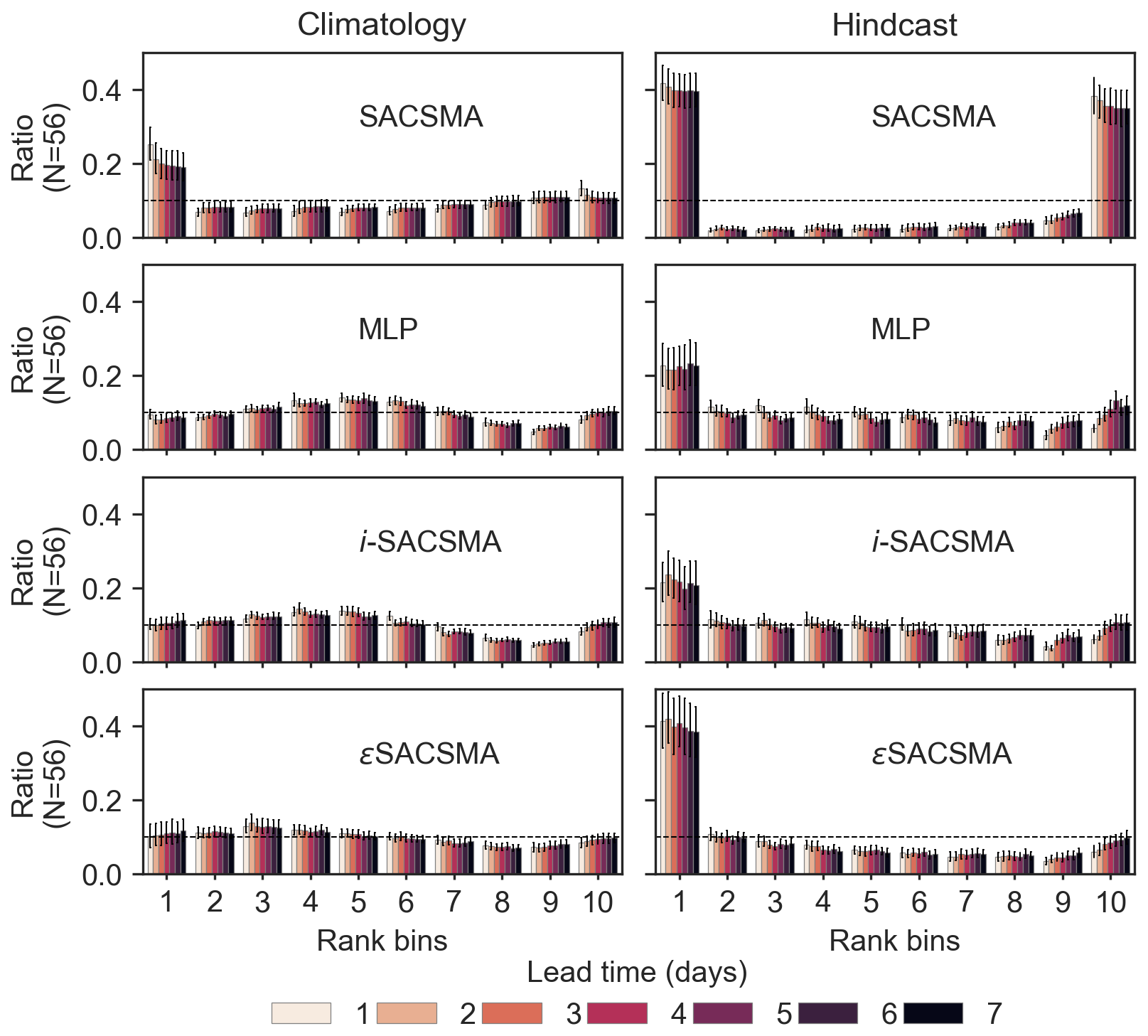
Figure B3 Rank diagrams for the benchmark SACSMA-cases and the DA strategies. x axis (10 rank classes), y axis (proportion of observed values in each class), median ratio and error-bars indicating the distributions of the 56 basins. Colors indicate the lead times.

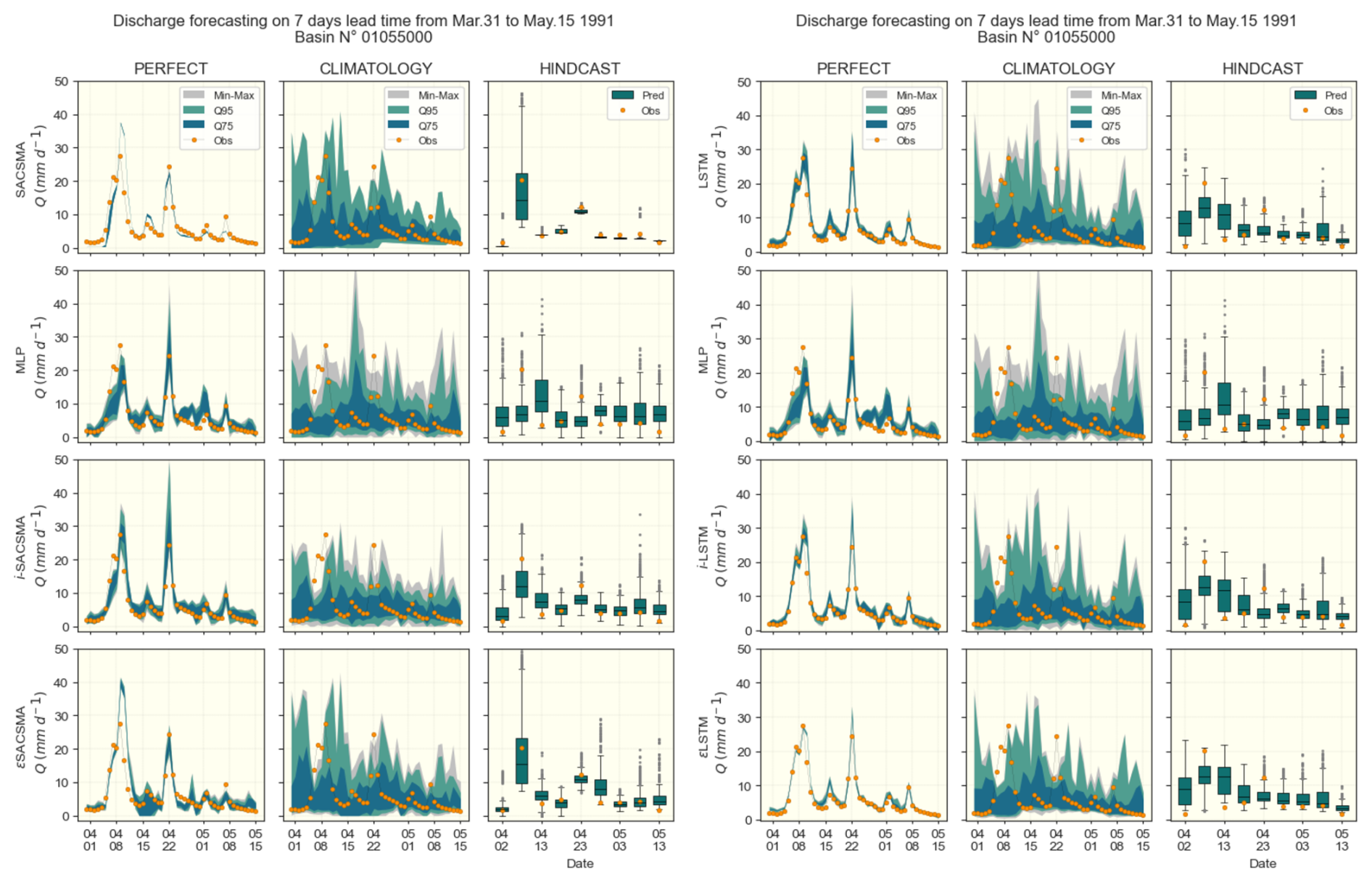
Figure B4 Example of hydrograph for 7 d lead times on the CAMELS-US dataset for both SACS-SMA (left panels) and LSTM (right panels) cases for basin No. 01055000.

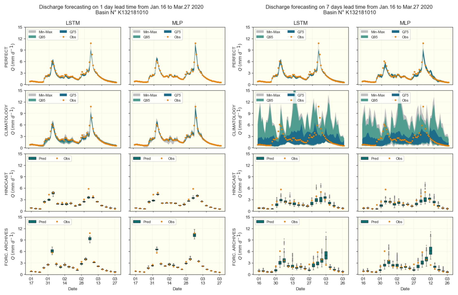
Figure B5 Example of hydrograph for 1 and 7 d lead times on the CAMELS-FR dataset for the basin K132181010.

Figure B6 Persistence scores for LSTM and the MLP (DA1) on the CAMELS-FR dataset.

Figure B7 SSR for the LSTM and the DA1 (MLP) with the CAMELS-FR dataset.

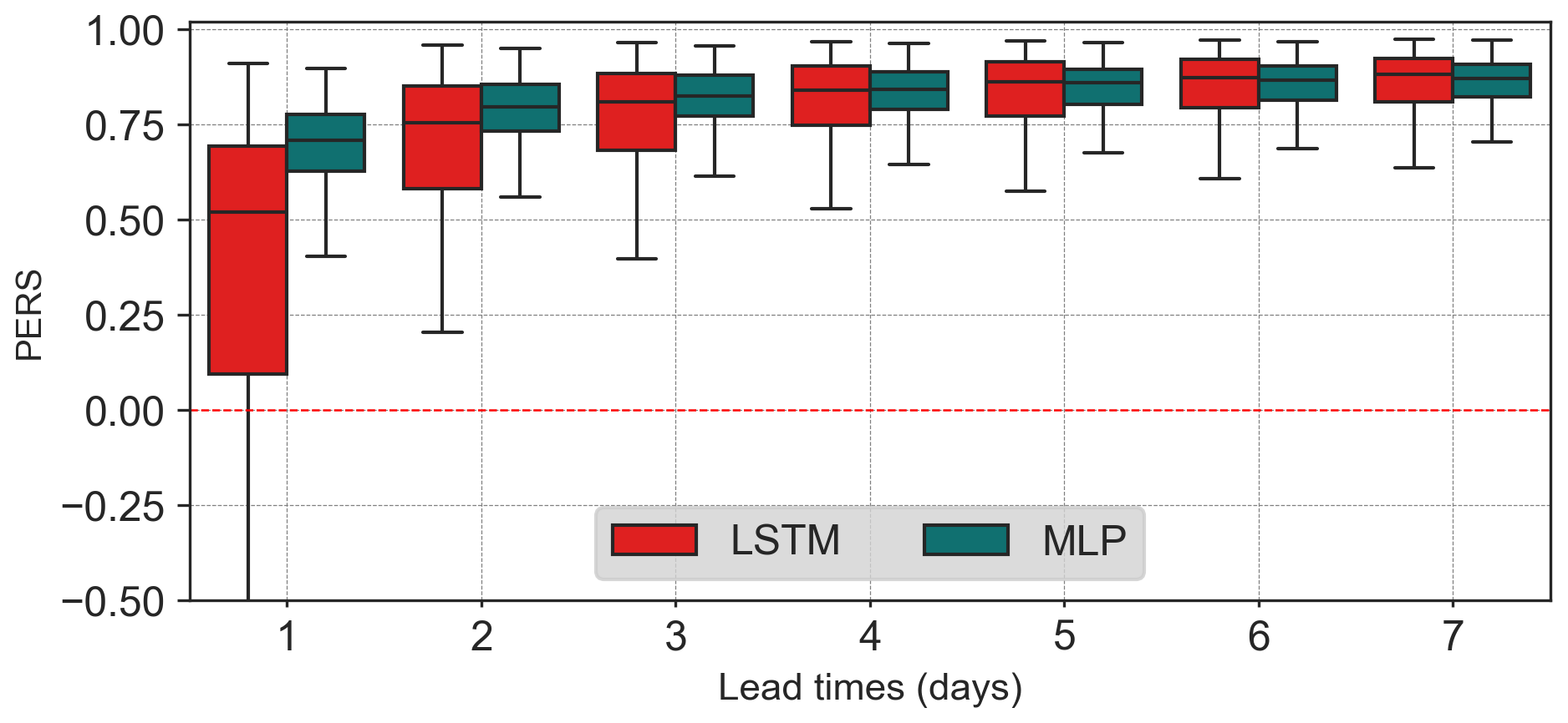
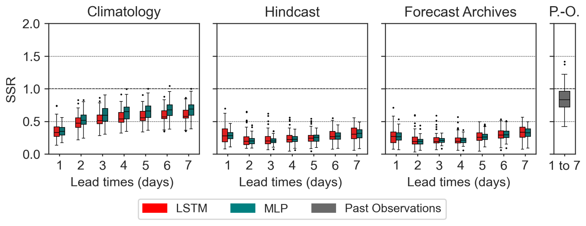
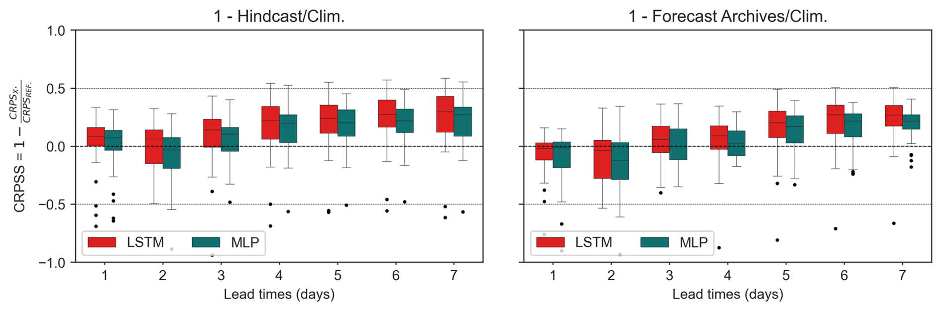
Figure B8 CRPSS of forecast products against the Climatology-based scenario for the CAMELS-FR dataset.

Figure B9 AUC scores for the LSTM and the DA1 (MLP) with the CAMELS-FR dataset.